Online Distributed Learning over Random Networks

Abstract

The recent deployment of multi-agent systems in a wide range of scenarios has enabled the solution of learning problems in a distributed fashion. In this context, agents are tasked with collecting local data and then cooperatively train a model, without directly sharing the data. While distributed learning offers the advantage of preserving agents’ privacy, it also poses several challenges in terms of designing and analyzing suitable algorithms. This work focuses specifically on the following challenges motivated by practical implementation: (i) online learning, where the local data change over time; (ii) asynchronous agent computations; (iii) unreliable and limited communications; and (iv) inexact local computations. To tackle these challenges, we introduce the Distributed Operator Theoretical (DOT) version of the Alternating Direction Method of Multipliers (ADMM), which we call the DOT-ADMM Algorithm. We prove that it converges with a linear rate for a large class of convex learning problems (e.g., linear and logistic regression problems) toward a bounded neighborhood of the optimal time-varying solution, and characterize how the neighborhood depends on (i)–(iv). We corroborate the theoretical analysis with numerical simulations comparing the DOT-ADMM Algorithm with other state-of-the-art algorithms, showing that only the proposed algorithm exhibits robustness to (i)–(iv).

Distributed learning, online learning, asynchronous networks, unreliable communications, ADMM

1 Introduction

In recent years, significant technological advancements have enabled the deployment of multi-agent systems across various domains, including robotics, power grids, and traffic networks [1, 2]. These systems consist of interconnected agents that leverage their computational and communication capabilities to collaborate in performing assigned tasks. Many of these tasks – such as estimation [3, 4], coordination and control [5, 6, 7], resilient operation [8, 9, 10], and learning [11, 12, 13] – can be formulated as distributed optimization problems, see [2, 14, 15] for some recent surveys. In this context, this work focuses specifically on distributed optimization algorithms for learning under network constraints.

Traditional machine learning methods require transmitting all the data collected by the agents to a single location, where they are processed to train a model. However, communicating raw data exposes agents to privacy breaches, which is inadmissible in many applications such as healthcare and industry [16]. Moreover, it is often the case that the agents collect new data over time, which requires another round of data transmission and, as a result, both an increased privacy vulnerability and the need of repeating the centralized training task. In the alternative approach of distributed learning, the agents within the network first process their data to compute an approximate local model, and then refine such model by sharing it with their peers and agreeing upon a common model that better fits all the distributed data sets, with the goal of improving the overall accuracy. This strategy, however, poses some practical challenges – discussed in the next subsection – both at the computation level, such as different speed and precision computing, and at the communication level, such as loss and corruption of packets.

The focus of this paper is thus on solving online learning problems in a distributed way while addressing these practical challenges, which are discussed in detail in the next Section 1.1. In principle, different approaches developed in the distributed optimization literature can be applied to this problem, which are reviewed in Section 1.2. This paper introduces a distributed operator theoretical (DOT) version of the alternate direction method of multipliers (ADMM), which we call the DOT-ADMM Algorithm. Section 1.3 outlines how the DOT-ADMM advances the state-of-the-art thanks to its unique set of features and advantages, which are supported by novel theoretical results on stochastic operators.

1.1 Practical challenges in distributed learning

Asynchronous agents computations. The agents cooperating for the solution of a learning problem are oftentimes highly heterogeneous, in particular in terms of their computational resources [16]; consequently, the agents may perform local computations at different rates. The simple solution of synchronizing the network by enforcing that all agents terminate the $k$-th local computation at iteration $k$ entails that better-performing agents must wait for the slower ones (cf. [17, Fig. 2]). Therefore, in this paper we allow the agents to perform local processing at their own pace, which is a more efficient strategy than enforcing synchronization.

Unreliable communications. In real-world scenarios, the agents have at their disposal imperfect channels to deliver the locally processed models to their peers. One problem that may occur, particularly when relying on wireless communications, is that transmissions from one agent to another may be lost in transit (e.g., due to interference [12]). When a transmission is lost, the newly processed local model of an agent is not delivered to its neighboring agents, and the algorithms need to be robust to this occurrence. A second problem that must be faced, especially when the local models stored by the agents are high dimensional, is the impracticability of sharing the exact local model over limited channels (e.g., when training a deep neural network). To satisfy limited communications constraints, different approaches have been explored, foremost of which is quantization/compression of the messages exchanged by the agents [13]. But quantizing a communication implies that an inexact version of the local models is shared by the agents, which can be seen as a disturbance in the communication. Therefore, we consider both packet-loss and packet-corruption during the communications between agents, which allow us to deal with the two above-mentioned problems.

Inexact local computations. In learning applications, the local costs of the agents are often defined on a large number of data points. Computing the gradient (or, as will be the case of the proposed algorithm, the proximal) of the costs may thus be impractical, particularly in an online set-up in which agents can process local data only in the interval of time $[k,k+1)$. To solve this issue, so-called stochastic gradients are employed, which construct an approximation of the local gradients using a limited number of data points [18]. This implies that every time a stochastic gradient is applied by an agent, some error is introduced in the algorithm. As mentioned above, the proposed algorithm needs to compute the proximal of the local cost function. However, unless the cost is proximable [19] and there is a closed form, the proximal needs to be computed via an iterative scheme, such as gradient descent. But again due to the limited computational time $[k,k+1)$ allowed to the agent, the proximal can be computed only with a limited number of iterations, introducing an approximation. The issue may be further compounded by the use of stochastic gradients instead of full gradients.

1.2 Distributed learning review

Among the numerous and various approaches proposed in the state-of-the-art, the pioneering algorithms are those based on (sub)gradient methods [2], which however require the use of diminishing step-sizes to guarantee convergence, and thus are not compatible with asynchronous computations. Another class of suitable algorithms is that of gradient tracking, which can achieve convergence with the use of fixed step-sizes [20]. On the one hand, different gradient tracking methods have been proposed for application in an online learning context, see e.g. [21, 22]. On the other, the use of robust average consensus techniques has also enabled the deployment of gradient tracking for learning under the constraints of Section 1.1, see e.g. [23, 24, 25, 26, 27]. However, gradient tracking algorithms may suffer from a lack of robustness to some of these challenges [28].

Our approach falls in a different branch of research, which is based on the alternating direction method of multipliers (ADMM). ADMM-based algorithms have turned out to be reliable and versatile for distributed optimization [11, 29]. In particular, ADMM has been shown to be robust to asynchronous computations [30, 31, 29], packet losses [32], and both [33]. Additionally, its convergence with inexact communications has been analyzed in [34], and the impact of inexact local computations has been studied in [35]. Moreover, the convergence of ADMM-based algorithm under network constraints has been usually shown to occur at a sub-linear rate, whereas a linear rate can be proved only under additional assumptions, such as strong convexity [33]).

Instead, the algorithm we propose is shown to converge with a linear rate without the strong convexity assumption, but under a milder set of assumptions, while facing at the same time all the challenges described in Section 1.1.

1.3 Main contributions

The proposed DOT-ADMM Algorithm has the following set of features:

• Convergence with a linear rate for linear and logistic regression problems;

• Applicability in an online scenario where the data sets available to the agents change over time;

• Robustness to asynchronous and inexact computations of the agents;

• Robustness to unreliable communications.

The main theoretical results of the paper are as follows:

• The first main result is that of proving linear convergence (in mean) to a neighborhood of the set of fixed points for a special class of time-varying stochastic operators defined by averaged and metric subregular operators (see Theorem 3). Such a neighborhood is formally described and it is shown to be almost surely reached asymptotically. Current results in the state-of-the-art can only guarantee sub-linear convergence without the additional assumption property of metric subregularity [36]. When metric subregularity does not hold everywhere but only in a subset of the state space, it is shown that the above-described results hold eventually after a finite time (see Theorem 4).

• The second main result shows that if the proposed DOT-ADMM Algorithm is employed to solve convex distributed optimization problems and if the associated operator is metric subregular, then the distance to a neighborhood of the time-varying set of optimal solutions converges linearly (in mean) and the neighborhood is almost surely reached asymptotically (see Theorem 1). The main novelty of this result relies on the fact that it is not required that the optimization problem is strongly convex, as previous results do [37, 38, 39, 33]. Complimentary results are provided for simpler scenarios where some of the challenges addressed do not come into play (see Corollary 1) and for the case in which metric subregularity holds in a subset of the state space (see Theorem 2).

• The last but most practical result consists in showing how metric subregularity can be verified for standard learning problems, such as linear regression (see Proposition 1) and logisitc regression (see Proposition 2). These results can be also used as tutorial examples for other learning problems with different regression models. The performance of the DOT-ADMM Algorithm is evaluated for the more complex logistic regression problem, which is also compared with that of gradient tracking algorithms, usually employed in this scenario [25, 26]. Simulations reveal that the DOT-ADMM Algorithm outperforms gradient tracking algorithms, showing high resilience to all the above-discussed challenges at the same time.

1.4 Outline

Section 2 provides the notation used throughout the paper and useful preliminaries on graph theory and operator theory. In Section 3 we first formalize the problem of distributed learning and state our main working assumptions, then we describe the proposed DOT-ADMM Algorithm and discuss its convergence properties. Section 4 is devoted to the proof of the convergence result anticipated in Section 3, which relies on a novel foundational result on stochastic operators that are metric subregular. Section 5 outlines how the proposed algorithm can be applied to different learning problems, with a focus on linear and logistic regression problems. In Section 6 several numerical results are carried out, and Section 7 gives some concluding remarks.

2 Problem formulation

2.1 Notation and preliminaries

The set of real and integer numbers are denoted by $\mathbb{R}$ and $\mathbb{Z}$, respectively, while $\mathbb{R}_{+}$ and ${\rm Nature}$ denote their restriction to positive entries. Matrices are denoted by uppercase letters, vectors and scalars by lowercase letters, while sets and spaces are denoted by uppercase calligraphic letters. The identity matrix is denoted by $I_{n}$, $n\in{\rm Nature}$, while the vectors of ones and zeros are denoted by $\mathbbold{1}_{n}$ and $\mathbbold{0}_{n}$; subscripts are omitted if clear from the context. Maximum and minimum of an $n$-element vector ${u=[u_{1},\ldots,u_{n}]^{\top}}$, are denoted by $\overline{u}=\max_{i=1,\ldots,n}u_{i}$ and $\underline{u}=\min_{i=1,\ldots,n}u_{i}$, respectively. The Kronecker product between two vectors $x,y\in\mathbb{R}^{n}$ is denoted by the symbol $\otimes$ and is defined component-wise by $(x\otimes y)_{i}=x_{i}y_{i}$ for $i=1,\ldots,n$.

Networks and graphs - We consider networks modeled by undirected graphs ${\mathcal{G}=(\mathcal{V},\mathcal{E})}$, where $\mathcal{V}=\{1,\ldots,n\}$, $n\in{\rm Nature}$, is the set of nodes, and $\mathcal{E}\subseteq\mathcal{V}\times\mathcal{V}$ is the set of edges connecting the nodes. An undirected graph $\mathcal{G}$ is said to be connected if there exists a sequence of consecutive edges between any pair of nodes $i,j\in\mathcal{V}$. Nodes $i$ and $j$ are neighbors if there exists an edge ${(i,j)\in\mathcal{E}}$. The set of neighbors of node $i$ is denoted by $\mathcal{N}_{i}=\left\{j\in\mathcal{V}:(i,j)\in\mathcal{E}\right\}$. For the sake of simplicity, we consider graphs with self-loops, i.e., $i\in\mathcal{N}_{i}$, and denote by $\eta_{i}=|\mathcal{N}_{i}|$ the number of neighbors and by $\xi=2|\mathcal{E}|=\eta_{1}+\cdots+\eta_{n}$ twice the number of undirected edges in the network.

Operator theory - We introduce some key notions from operator theory in finite-dimensional euclidean spaces, i.e., vector spaces $\mathbb{R}^{n}$ with ${\left|\kern-1.07639pt\left|\cdot\right|\kern-1.07639pt\right|}$ and distance $d$

$${\left|\kern-1.07639pt\left|x\right|\kern-1.07639pt\right|}=\sqrt{x^{\top}x},\qquad d(x,y)={\left|\kern-1.07639pt\left|x-y\right|\kern-1.07639pt\right|}.$$

Operators $\mathsf{F}:\mathbb{R}^{n}\rightarrow\mathbb{R}^{n}$ are denoted with block capital letters. An operator is affine if there exist a matrix $A\in\mathbb{R}^{n\times n}$ and a vector $b\in\mathbb{R}^{n}$ such that ${\mathsf{F}:x\mapsto Ax+b}$, and linear if $b=\mathbbold{0}$. The linear operator associated to the identity matrix $I$ is defined by ${\mathsf{Id}:x\mapsto Ix}$. Given $\mathsf{F}:\mathbb{R}^{n}\rightarrow\mathbb{R}^{n}$, ${\operatorname{fix}(\mathsf{F})=\{x\in\mathbb{R}^{n}:\mathsf{F}(x)=x\}}$ denotes its set of fixed points. The distance of a point $x$ from a set $\mathcal{X}$ is defined by

$$d_{\mathcal{X}}(x)=\inf_{y\in\mathcal{X}}{\left|\kern-1.07639pt\left|x-y\right|\kern-1.07639pt\right|}.$$

When $\mathcal{X}$ is the set of fixed points of an operator $\mathsf{F}$, we use the shorthand notation $d_{\mathsf{F}}$ instead of $d_{\operatorname{fix}(\mathsf{F})}$. With this notation, we now define some operator-theoretical properties of operators, which are pivotal in this paper.

      Definition 1.

An operator $\mathsf{F}:\mathbb{R}^{n}\to\mathbb{R}^{n}$ is metric subregular if there is a positive constant $\gamma>0$ such that

$$d_{\mathsf{F}}(x)\leq\gamma{\left|\kern-1.07639pt\left|(\mathsf{Id}-\mathsf{F})x\right|\kern-1.07639pt\right|},\qquad\forall x\in\mathbb{R}^{n}.$$ (1)

      Definition 2.

An operator $\mathsf{F}:\mathbb{R}^{n}\to\mathbb{R}^{n}$ is nonexpansive if

$${\left|\kern-1.07639pt\left|\mathsf{F}(x)-\mathsf{F}(y)\right|\kern-1.07639pt\right|}\leq{\left|\kern-1.07639pt\left|x-y\right|\kern-1.07639pt\right|},\qquad\forall x,y\in\mathbb{R}^{n}.$$

Moreover, the operator $\mathsf{G}:=(1-\alpha)\mathsf{Id}+\alpha\mathsf{F}$ with $\alpha\in(0,1)$ is $\alpha$-averaged if $\mathsf{F}$ is nonexpansive, or, equivalently, if

$${\left|\kern-1.07639pt\left|\mathsf{G}(x)-\mathsf{G}(y)\right|\kern-1.07639pt\right|}^{2}\leq{\left|\kern-1.07639pt\left|x-y\right|\kern-1.07639pt\right|}^{2}-\frac{1-\alpha}{\alpha}{\left|\kern-1.07639pt\left|(\mathsf{Id}-\mathsf{G})(x)-(\mathsf{Id}-\mathsf{G})(y)\right|\kern-1.07639pt\right|}^{2}.$$

Let $\Gamma_{0}^{n}$ be the set of proper, lower semicontinuous, convex functions from $\mathbb{R}^{n}$ to $\mathbb{R}\cup\{+\infty\}$. Then, given $f\in\Gamma_{0}^{n}$, the proximal operator of $f$ is defined by

$$\operatorname{prox}^{\rho}_{f}(y)=\operatorname*{\arg\!\min}_{x}\left\{f(x)+\frac{1}{2\rho}{\left|\kern-1.07639pt\left|x-y\right|\kern-1.07639pt\right|}^{2}\right\},$$

where $\rho>0$ is a penalty parameter; if $\rho=1$, it is omitted. The proximal operator is $1/2$-averaged.

2.2 The problem

We consider a network of $n$ agents linked according to an undirected, connected graph ${\mathcal{G}=(\mathcal{V},\mathcal{E})}$. Each agent $i\in\mathcal{V}$ has a vector state ${x_{i}(k)\in\mathbb{R}^{p}}$ with $p\in{\rm Nature}$, and has access to a time-varying local cost $f_{i,k}:\mathbb{R}^{p}\to\mathbb{R}\cup\{+\infty\}$, $k\in{\rm Nature}$. The objective of the network is to solve the optimization problem:

$$\min_{x_{i}}\sum_{i\in\mathcal{V}}f_{i,k}(x_{i})$$ (2a)

$$\text{s.t.}\ x_{i}=x_{j}\ \text{if}\ (i,j)\in\mathcal{E}$$ (2b)

whose set of solutions is denoted by $\mathcal{X}^{*}_{k}$. We make the following two standing assumptions, which are standard assumptions in online optimization [41].

      Assumption 1.

At each time $k\in{\rm Nature}$, the local cost functions $f_{i,k}$ of problem (2) are proper, lower semi-continuous, and convex, i.e., $f_{i,k}\in\Gamma_{0}^{p}$.

      Assumption 2.

The set of solutions $\mathcal{X}^{*}_{k}$ to problem (2) are non-empty at each time $k\in{\rm Nature}$. In addition, the minimum distance between two solutions $x^{*}(k)\in\mathcal{X}^{*}_{k}$ at consecutive times is upper-bounded by a nonnegative constant $\sigma\geq 0$, i.e.,

$$\inf_{k\in{\rm Nature}}{\left|\kern-1.07639pt\left|x^{*}(k)-x^{*}(k-1)\right|\kern-1.07639pt\right|}\leq\sigma.$$

      Remark 1.

Under Assumption 1 the set of solutions $\mathcal{X}_{k}^{*}$ to problem (2) is convex (see [40, Proposition 11.6]) but not necessarily closed nor bounded. Consequently, the solution is not necessarily unique.

The dynamic nature of the problem implies that the solution – in general – cannot be reached exactly, but rather that the agents’ states will reach a neighborhood of it [42, 41]. Our goal is thus to quantify how closely the agents can track the optimal solution over random networks, which are characterized by the following challenging conditions, as discussed in Section 1.1:

• asynchronous agents computations;

• unreliable communications;

• inexact local computations.

The next section introduces the proposed algorithm along with the formal description of the above challenges and the main working assumptions.

3 Proposed algorithm and convergence results

To solve the problem in eq. (2), we employ the Distributed Operator Theoretical (DOT) version of the Alternating Direction Method of Multipliers (ADMM), called DOT-ADMM Algorithm (see [33] and references therein), which is derived by applying the relaxed Peaceman-Rachford splitting method to the dual of problem in eq. (2), and its distributed implementation is detailed in Algorithm 1.

Each agent $i\in\mathcal{V}$ first updates its local state $x_{i}\in\mathbb{R}^{p}$ according to eq. (4), then sends some information to each neighbor $j\in\mathcal{N}_{i}$ within the packet $y_{i\to j}$. The agents are assumed to be heterogeneous in their computation capabilities, therefore at each time step only some of the agents are ready for the communication phase. In turn, after receiving the information from its neighbors, each agent updates its auxiliary state variables $z_{ij}\in\mathbb{R}^{p}$ with $j\in\mathcal{N}_{i}$ according to eq. (5). Note that the local update in eq. (4) depends only on information available to agent $i$, while for the auxiliary update in eq. (5) the agent needs to first receive the aggregate information $y_{j\to i}(k)$ from the neighbor $j$.

The DOT-ADMM Algorithm makes also explicit where the sources of stochasticity discussed in Section 1.1 come into play: asynchronous agents’ computations and packet-loss prevent the updates in eqs. (4)-(5) to be performed at each time $k\in{\rm Nature}$, whereas inexact local computations and noisy communications make these updates inaccurate. We model these sources of stochasticity by means of the following random variables:

• ${\beta_{ij}(k)\sim\text{Ber}(\rho_{ij})}$ are Bernoulli random variables with $\rho_{ij}\in(0,1]$ modeling the asynchronous agents’ computations and packet-loss: $p_{ij}$ denotes the probability that agent $j$ has completed its computation and packet $y_{j\to i}$ successfully arrives to agent $i$;

• $u_{i}(k)$ and $v_{ij}(k)$ are i.i.d. random variables which represent, respectively, the additive error modeling inexact local updates of $x_{i}$ and noisy transmission of $y_{j\to i}(k)$ sent by node $j$ to node $i$.

With these definitions in place, we define the perturbed variables as follows

$$\widetilde{x}_{i}(k) =x_{i}(k)+u_{i}(k)$$

$$\widetilde{z}_{ij}(k) =z_{ij}(k)+\alpha v_{ij}(k)$$

One can further notice that the additive error $u_{i}(k)$ on $x_{i}(k)$ is also an additive error on $y_{j\to i}$ (scaled by a factor equal to $2\rho$). Therefore, one can consider only one source of error $e_{ij}=v_{ij}(k)+2\rho u_{i}(k)$ and write the perturbed updates as

$$x_{i}(k) =\mathsf{F}_{i,k}(\widetilde{z}(k-1))$$ (3a)

$$\widetilde{z}_{ij}(k) =\begin{cases}\mathsf{T}_{ij,k}(\widetilde{z}(k-1))+\alpha e_{ij}(k)&\text{if }\beta_{ij}(k)=1\\ \widetilde{z}_{ij}(k-1)&\text{otherwise}\end{cases}$$ (3b)

where the operators $\mathsf{F}_{i,k}$, $\mathsf{T}_{ij,k}$ are those of eqs. (4)-(5).

Algorithm 1 Distributed Operator Theoretical (DOT) ADMM

For each agent $i\in\mathcal{V}$ initialize the auxiliary variables $\{z_{ij}(0)\}_{j\in\mathcal{N}_{i}}$; choose the relaxation $\alpha\in(0,1)$ and the penalty $\rho>0$.

Each agent returns $x_{i}(k)$ that is an (approximated) solution to the distributed optimization problem in eq. (2).

for $k=1,2,\ldots$ each active agent $i\in\mathcal{V}$

// asynchronous computations and inexact updates

receives a local cost $f_{i,k}$ and applies the local update

$$x_{i}(k)=\operatorname{prox}_{f_{i,k}}^{1/\rho\eta_{i}}\left(\frac{1}{\rho\eta_{i}}\sum_{j\in\mathcal{N}_{i}}z_{ij}(k-1)\right)$$ (4)

for each agent $j\in\mathcal{N}_{i}$ 

     transmits the packet

$$y_{i\to j}(k)=2\rho x_{i}(k)-z_{ij}(k-1).$$

end for

for each packet $y_{j\to i}$ received by agent $j\in\mathcal{N}_{i}$ 

     // noisy communications with packet loss

     updates the auxiliary variable

$$z_{ij}(k)=(1-\alpha)z_{ij}(k-1)+\alpha y_{j\to i}(k),$$ (5)

end for

end for

With this notation, we formalize next the challenging assumptions under which the problem in eq. (2) must be solved.

      Assumption 3.

At each time step, each node $j$ has completed its local computation and successfully transmits data to its neighbors $i\in\mathcal{N}_{j}$ with probability $\rho_{ij}\in(0,1]$.

      Assumption 4.

Each node $i\in\mathcal{V}$ updates its local variable $x_{i}(k)$ with an additive error ${u_{i}(k)\in\mathbb{R}^{p}}$ and receives information from neighbor $j\in\mathcal{N}_{i}$ with an additive noise ${v_{ij}(k)\in\mathbb{R}^{p}}$ such that the overall error ${e_{ij}(k)=v_{ij}(k)+2\rho u_{i}(k)}$ on the update of the auxiliary variable $z_{ij}(k)$ is bounded by ${\mathbb{E}\left[{\left|\kern-1.07639pt\left|e_{ij}(k)\right|\kern-1.07639pt\right|}\right]\leq\nu_{e}<\infty}$.

3.1 Convergence results

For the convenience of the reader, we state next our main results, while we postpone their proofs to Sections 4.2-4.3, since they require several intermediate developments on stochastic operators discussed in Section 4.1.

We begin with the following theorem, which characterizes the mean linear convergence of DOT-ADMM in the stochastic scenario described in Section 1.1 and formalized in Section 3.

      Theorem 1       (Linear convergence).

Consider the online distributed optimization in problem (2) under Assumptions 1-2, and a connected network of agents that solves it by running the DOT-ADMM Algorithm under Assumptions 3-4. If:

• the map $\mathsf{T}_{k}$ defined block-wise by $\mathsf{T}_{ij,k}$ as in eq. (5) is metric subregular;

then the following results for the distance between $x(k)$ and the set of solutions $\mathcal{X}_{k}^{*}$ to problem (2) hold:

• there is an upper bound for $d_{\mathcal{X}_{k}^{*}}(x(k))$ that holds in mean for all $k\in{\rm Nature}$, and this bound has a linearly decaying dependence on the initial condition;

• there is an upper bound for $d_{\mathcal{X}_{k}^{*}}(x(k))$ that holds almost surely when $k\to\infty$, and this bound does not depend on the initial condition.

The following corollary makes explicit how the results of Theorem 1 simplifies for some simpler scenarios.

      Corollary 1       (Particular cases).

Consider the scenario of Theorem 1. If the cost functions $f_{i,k}=f_{i}$ are static and there are no sources of additive error, then, letting $\mathcal{X}^{*}$ be the set of solutions to problem in eq. (2):

• the distance of $x(k)$ from $\mathcal{X}^{*}$ converges linearly to zero in mean;

• $x(k)$ almost surely converges to $\mathcal{X}^{*}$ when $k\to\infty$.

If further the communications are synchronous and reliable, then

• $x(k)$ converges linearly and almost surely to $\mathcal{X}^{*}$.

We conclude with another result showing that eventual linear convergence can be proved for strongly convex and smooth costs; this result subsumes that of [33], proving it in a more general scenario.

      Theorem 2       (Eventual linear convergence).

Consi-der a static instance of the distributed optimization in problem (2) over a connected network of agents that solves it by running the DOT-ADMM Algorithm under Assumptions 3-4. If the costs are strongly convex and twice continuously differentiable, then:

• there is a finite time $k^{*}\in{\rm Nature}$ such that for $k\geq k^{*}$ results $i)$ and $ii)$ of Theorem 1 hold.

4 Proofs of the Convergence Results

In this section, we first provide general convergence results for stochastic metric subregular operators, which we then leverage to prove the convergence results of Section 3.1.

4.1 Foundational convergence results

The goal of this section is to prove the eventual linear convergence (in mean) of a special class of time-varying stochastic operators defined by $\alpha$-averaged and $\gamma$-metric subregular operators. In particular, we are interested in operators of the form of eq. (6), which have been proven to be convergent in mean (but sub-linearly) by Combettes and Pesquet [36], under the assumption of $\alpha$-averagedness and diminishing errors.

      Theorem 3.

Let ${\widetilde{\mathsf{T}}^{e}_{k}:\mathbb{R}^{m}\rightarrow\mathbb{R}^{m}}$ be a time-varying operator defined component-wise by

$$\widetilde{\mathsf{T}}^{e}_{\ell,k}(z):=\begin{cases}\mathsf{T}_{\ell,k}(z)+e_{\ell,k}&\text{if }\beta_{\ell,k}=1\\ z_{\ell}&\text{otherwise}\end{cases}$$ (6)

for $\ell=1,\ldots,m$, where $e_{\ell,k}$ are i.i.d. random variables and ${\beta_{\ell,k}\sim\emph{\text{Ber}}(\rho_{\ell})}$ are Bernoulli i.i.d. random variables such that $\rho_{\ell}\in(0,1]$. If it holds:

• $\exists\sigma>0$ such that $d_{\mathsf{T}_{k}}(z^{*})\leq\sigma$ for ${z^{*}\in\operatorname{fix}(\mathsf{T}_{k-1})}$;

• ${\mathsf{T}_{k}}$ is $\alpha$-averaged;

• $\mathsf{T}_{k}$ is $\gamma$-metric subregular;

then the iteration $z(k)=\widetilde{\mathsf{T}}^{e}_{k}(z(k-1))$ converges linearly in mean according to

$$\mathbb{E}\left[d_{\mathsf{T}_{k}}(z(k))\right]\leq\sqrt{\frac{\overline{p}}{\underline{p}}}\left[\mu^{k}d_{\mathsf{T}_{0}}(z(0))+\sum_{h=1}^{k}\mu^{k-h}(\mathbb{E}\left[{\left|\kern-1.07639pt\left|e_{h}\right|\kern-1.07639pt\right|}\right]+\mu\sigma)\right]$$

and it almost surely holds that

$$\limsup_{k\to\infty}d_{\mathsf{T}_{k}}(z(k))\leq\lim_{k\to\infty}\sqrt{\frac{\overline{p}}{\underline{p}}}\sum_{h=1}^{k}\mu^{k-h}(\mathbb{E}\left[{\left|\kern-1.07639pt\left|e_{h}\right|\kern-1.07639pt\right|}\right]+\mu\sigma),$$

where

$$\mu=\sqrt{1-\frac{(1-\alpha)\underline{p}}{\alpha\lambda}},\quad\lambda>\max\left\{\gamma^{2},\frac{(1-\alpha)\underline{p}}{\alpha}\right\}.$$ (7)

Proof.

[Punctual upper bound] - We make use of the so-called diagonally-weighted norm in the sense of [43], where the vector of nonnegative weights is the vector of probabilities $p=[p_{1},\ldots,p_{m}]^{\top}$, which is defined next

$${\left|\kern-1.29167pt\left|\kern-1.29167pt\left|z\right|\kern-1.29167pt\right|\kern-1.29167pt\right|}^{2}=\sum_{\ell=1}^{m}\frac{1}{p_{\ell}}z_{\ell}^{2},$$ (8)

following the usual notation in our community [36]. Clearly, such a norm satisfies the following

$$\underline{p}{\left|\kern-1.29167pt\left|\kern-1.29167pt\left|z\right|\kern-1.29167pt\right|\kern-1.29167pt\right|}^{2}\leq{\left|\kern-1.07639pt\left|z\right|\kern-1.07639pt\right|}^{2}\leq\overline{p}{\left|\kern-1.29167pt\left|\kern-1.29167pt\left|z\right|\kern-1.29167pt\right|\kern-1.29167pt\right|}^{2}.$$ (9)

Similarly to the Euclidean distance $d_{\mathsf{T}_{k}}(z)$ from the set of fixed points of $\mathsf{T}$, we define the distance ${d_{\mathsf{T}_{k}}^{\prime}(z)=\inf_{y\in\operatorname{fix}(\mathsf{T}_{k})}{\left|\kern-1.29167pt\left|\kern-1.29167pt\left|z-y\right|\kern-1.29167pt\right|\kern-1.29167pt\right|}}$, such that

$$\frac{1}{\overline{p}}d_{\mathsf{T}_{k}}(z)^{2}\overset{(i)}{\leq}d_{\mathsf{T}_{k}}^{\prime}(z)^{2}\overset{(i)}{\leq}\frac{1}{\underline{p}}d_{\mathsf{T}_{k}}(z)^{2}\overset{(ii)}{\leq}\frac{\gamma^{2}}{\underline{p}}{\left|\kern-1.07639pt\left|(\mathsf{Id}-\mathsf{T}_{k})z\right|\kern-1.07639pt\right|}^{2},$$ (10)

where (i) follow by the definition of projection and eq. (9), whereas (ii) by $\gamma$-metric subregularity of $\mathsf{T}_{k}$. We also conveniently rewrite the operator $\widetilde{\mathsf{T}}^{e}_{k}$ in eq. (6) by

$$z_{\ell}(k)=\widetilde{\mathsf{T}}^{e}_{\ell,k}(z(k-1))=\widetilde{\mathsf{T}}_{\ell,k}(z(k-1))+\beta_{\ell,k}e_{\ell,k},$$

where

$$\widetilde{\mathsf{T}}_{\ell,k}(z(k-1))=z_{\ell}(k-1)+\beta_{\ell,k}(\mathsf{T}_{\ell,k}(z(k-1))-z_{\ell}(k-1)).$$

Letting $\boldsymbol{e}\in\mathbb{R}^{m}$ be the vector stacking all the errors and ${z^{*}_{k}\in\operatorname{fix}(\mathsf{T}_{k})}$, then by eq. (10) and the triangle inequality we can write

$$d^{\prime}_{\mathsf{T}_{k}}(z(k)) ={\left|\kern-1.29167pt\left|\kern-1.29167pt\left|z(k)-z^{*}_{k}\right|\kern-1.29167pt\right|\kern-1.29167pt\right|}$$

$$={\left|\kern-1.29167pt\left|\kern-1.29167pt\left|\widetilde{\mathsf{T}}^{e}_{k}(z(k-1))-z^{*}_{k}\right|\kern-1.29167pt\right|\kern-1.29167pt\right|}$$

$$\leq{\left|\kern-1.29167pt\left|\kern-1.29167pt\left|\widetilde{\mathsf{T}}_{k}(z(k-1))-z^{*}_{k}\right|\kern-1.29167pt\right|\kern-1.29167pt\right|}+{\left|\kern-1.29167pt\left|\kern-1.29167pt\left|e_{k}\right|\kern-1.29167pt\right|\kern-1.29167pt\right|}$$

and thus

$$\mathbb{E}\left[d^{\prime}_{\mathsf{T}}(z(k))\right]\leq\mathbb{E}\left[{\left|\kern-1.29167pt\left|\kern-1.29167pt\left|\widetilde{\mathsf{T}}_{k}(z(k-1))-z^{*}_{k}\right|\kern-1.29167pt\right|\kern-1.29167pt\right|}\right]+\mathbb{E}\left[{\left|\kern-1.29167pt\left|\kern-1.29167pt\left|e_{k}\right|\kern-1.29167pt\right|\kern-1.29167pt\right|}\right].$$

We are interested in finding an upper-bound to the first term on the right-hand side of the above inequality, whose explicit form is given by

$${\left|\kern-1.29167pt\left|\kern-1.29167pt\left|\widetilde{\mathsf{T}}_{k}(z(k-1))-z^{*}_{k}\right|\kern-1.29167pt\right|\kern-1.29167pt\right|}^{2}=$$

$$=\sum_{\ell=1}^{m}\frac{1}{p_{\ell}}\Big{[}(1-\beta_{{\ell},k})z_{\ell}(k-1)+\beta_{\ell,k}\mathsf{T}_{\ell,k}(z(k-1))-z_{\ell,k}^{*})\Big{]}^{2}$$

$$=\sum_{\ell=1}^{m}\Big{[}\frac{1-\beta_{\ell,k}}{p_{\ell}}(z_{\ell}(k-1)-z_{\ell}^{*})^{2}+\frac{\beta_{\ell}}{p_{ij}}(\mathsf{T}_{\ell,k}(z(k-1))-z_{\ell,k}^{*})^{2}\Big{]}$$

where, since $\beta_{\ell,k}\in\{0,1\}$, we have used the following: ${\beta_{\ell,k}^{2}=\beta_{\ell,k}}$; ${(1-\beta_{\ell,k})^{2}=(1-\beta_{\ell,k})}$; ${(1-\beta_{\ell,k})\beta_{\ell,k}=0}$. An upper-bound to the conditional expectation w.r.t. the realizations of all r.v.s at time $k-1$ is given by

$$\mathbb{E}_{k-1}\left[{\left|\kern-1.29167pt\left|\kern-1.29167pt\left|\widetilde{\mathsf{T}}_{k}(z(k-1))-z^{*}_{k}\right|\kern-1.29167pt\right|\kern-1.29167pt\right|}^{2}\right]=$$

$$=\sum_{\ell=1}^{m}\left[\frac{1-p_{\ell}}{p_{\ell}}(z_{\ell}(k-1)-z_{\ell,k}^{*})^{2}+(\mathsf{T}_{\ell,k}(z(k-1))-z_{\ell,k}^{*})^{2}\right]$$

$$={\left|\kern-1.29167pt\left|\kern-1.29167pt\left|z(k-1)-z^{*}_{k}\right|\kern-1.29167pt\right|\kern-1.29167pt\right|}^{2}-{\left|\kern-1.07639pt\left|z(k-1)-z^{*}_{k}\right|\kern-1.07639pt\right|}^{2}+{\left|\kern-1.07639pt\left|\mathsf{T}_{k}(z(k-1))-z^{*}_{k}\right|\kern-1.07639pt\right|}^{2}$$

$$\overset{(i)}{\leq}{\left|\kern-1.29167pt\left|\kern-1.29167pt\left|z(k-1)-z^{*}_{k}\right|\kern-1.29167pt\right|\kern-1.29167pt\right|}^{2}-\frac{1-\alpha}{\alpha}{\left|\kern-1.07639pt\left|(\mathsf{Id}-\mathsf{T}_{k})z(k-1)\right|\kern-1.07639pt\right|}^{2}$$

$$\overset{(ii)}{\leq}d^{\prime}_{\mathsf{T}_{k}}(z(k-1))^{2}-\frac{1-\alpha}{\alpha}{\left|\kern-1.07639pt\left|(\mathsf{Id}-\mathsf{T}_{k})z(k-1)\right|\kern-1.07639pt\right|}^{2}$$

$$\overset{(iii)}{\leq}d^{\prime}_{\mathsf{T}_{k}}(z(k-1))^{2}-\frac{1-\alpha}{\alpha\gamma^{2}}\underline{p}d^{\prime}_{\mathsf{T}_{k}}(z(k-1))^{2}$$

$$=\left(1-\frac{(1-\alpha)\underline{p}}{\alpha\gamma^{2}}\right)d^{\prime}_{\mathsf{T}_{k}}(z(k-1))^{2}:=\mu^{2}d^{\prime}_{\mathsf{T}_{k}}(z(k-1))^{2}$$

where (i) holds by $\alpha$-averagedness, (ii) follows by selecting $z^{*}_{k}=\operatorname*{\arg\!\inf}_{y\in\operatorname{fix}(\mathsf{T}_{k})}{\left|\kern-1.29167pt\left|\kern-1.29167pt\left|z(k-1)-y\right|\kern-1.29167pt\right|\kern-1.29167pt\right|}$, and (iii) is a consequence of metric subregularity highlighted in eq. (10), and where $\mu\in(0,1)$ provided that $\gamma$ is sufficiently large, which we can always assume by overestimating the metric subregularity constant of $\mathsf{T}_{k}$, in particular by replacing $\gamma^{2}$ with $\lambda=\max\{\gamma^{2},(1-\alpha)\underline{p}/\alpha\}$ as in eq. (7).

Now, exploiting the (i) concavity of the square root, the (ii) Jensen’s inequality and the (iii) law of total expectation, we have

$$\mathbb{E}\Big{[}{\left|\kern-1.29167pt\left|\kern-1.29167pt\left|\cdot\right|\kern-1.29167pt\right|\kern-1.29167pt\right|}\Big{]}\overset{(i)}{=}\mathbb{E}\left[\sqrt{{\left|\kern-1.29167pt\left|\kern-1.29167pt\left|\cdot\right|\kern-1.29167pt\right|\kern-1.29167pt\right|}^{2}}\right]\overset{(ii)}{\leq}\sqrt{\mathbb{E}\left[{\left|\kern-1.29167pt\left|\kern-1.29167pt\left|\cdot\right|\kern-1.29167pt\right|\kern-1.29167pt\right|}^{2}\right]}\overset{(iii)}{=}\sqrt{\mathbb{E}\left[\mathbb{E}_{k-1}\left[{\left|\kern-1.29167pt\left|\kern-1.29167pt\left|\cdot\right|\kern-1.29167pt\right|\kern-1.29167pt\right|}^{2}\right]\right]}$$

which implies

$$\mathbb{E}\left[{\left|\kern-1.29167pt\left|\kern-1.29167pt\left|\widetilde{\mathsf{T}}_{k}(z(k-1))-z^{*}\right|\kern-1.29167pt\right|\kern-1.29167pt\right|}\right]\leq\mu\mathbb{E}\left[d_{\mathsf{T}}(z(k-1))\right].$$

Therefore we can write

$$\mathbb{E}\left[d^{\prime}_{\mathsf{T}_{k}}(z(k))\right]\leq\mu\mathbb{E}\left[d^{\prime}_{\mathsf{T}_{k}}(z(k-1))\right]+\mathbb{E}\left[{\left|\kern-1.29167pt\left|\kern-1.29167pt\left|e_{k}\right|\kern-1.29167pt\right|\kern-1.29167pt\right|}\right]$$

$$\qquad\overset{(i)}{\leq}\mu\mathbb{E}\left[d^{\prime}_{\mathsf{T}_{k-1}}(z(k-1))\right]+\frac{1}{\sqrt{\underline{p}}}\left(\mu\sigma+\mathbb{E}\left[{\left|\kern-1.07639pt\left|e_{k}\right|\kern-1.07639pt\right|}\right]\right)$$

where (i) holds by (9) and assumption i). Iterating we get

$$\begin{split}\mathbb{E}\left[d^{\prime}_{\mathsf{T}_{k}}(z(k))\right]&\leq\mu^{k}\mathbb{E}\left[d^{\prime}_{\mathsf{T}_{0}}(z(0))\right]+\\ &+\frac{1}{\sqrt{\underline{p}}}\sum_{h=1}^{k}\mu^{k-h}\left(\mu\sigma+\mathbb{E}\left[{\left|\kern-1.07639pt\left|e_{h}\right|\kern-1.07639pt\right|}\right]\right)\end{split}$$

and using (9) again yields the thesis.

[Asymptotic upper bound] - We use the same proof technique as in [44, Corollary 5.3]. Let us define

$$y(k)=\max\left\{0,d_{\mathsf{T}_{k}}(z(k))-\sqrt{\frac{\overline{p}}{\underline{p}}}\sum_{h=1}^{k}\mu^{k-h}({\left|\kern-1.07639pt\left|e_{h}\right|\kern-1.07639pt\right|}+\mu\sigma)\right\}$$

for which, by the previous result on the expected distance and Markov’s inequality, we have that for any $\varepsilon>0$

$$\mathbb{P}[y(k)\geq\varepsilon]\leq\frac{\mathbb{E}\left[y(k)\right]}{\varepsilon}\leq\frac{1}{\varepsilon}\sqrt{\frac{\overline{p}}{\underline{p}}}\mu^{k}d(z(0)),$$

and, summing over $k$ and using the geometric series,

$$\sum_{k=0}^{\infty}\mathbb{P}[y(k)\geq\varepsilon]\leq\frac{1}{\varepsilon}\sqrt{\frac{\overline{p}}{\underline{p}}}\frac{d(z(0))}{1-\mu}<\infty.$$

But by Borel-Cantelli lemma this means that

$$\limsup_{k\to\infty}y(k)\leq\varepsilon$$

almost surely; and since the inequality holds for any ${\varepsilon>0}$, the thesis follows.

      Remark 2.

The presence of random coordinate updates leads to a worse convergence rate $\mu$ compared to the convergence rate $\mu_{s}$ attained when all coordinates update at each iteration, indeed,

$$\mu_{s}=\sqrt{1-\frac{(1-\alpha)}{\alpha\lambda}}\leq\sqrt{1-\frac{(1-\alpha)\underline{p}}{\alpha\lambda}}=\mu,$$

with $\alpha\in(0,1)$ and $\lambda$ as in eq. (7). This is in line with the results proved in [36], and makes intuitive sense since the fewer updates are performed the slower the convergence.

We also provide a result to cover the case in which metric subregularity does not hold in the entire state space, but only in a subspace of it: this property is called locally metric subregularity.

      Theorem 4.

In the scenario of Theorem 3, if it holds:

• $\mathsf{T}_{k}=\mathsf{T}$ is not time-varying, i.e., $\sigma=0$;

• ${\mathsf{T}}$ is $\alpha$-averaged;

• $\mathsf{T}$ is metric subregular in a set $\mathcal{X}\subset\mathbb{R}^{n}$;

• $\lim_{k\rightarrow\infty}{\left|\kern-1.07639pt\left|e_{k}\right|\kern-1.07639pt\right|}\rightarrow 0$;

then it almost surely holds $\limsup_{k\to\infty}d_{\mathsf{T}}(z(k))=0.$ Moreover, there is a finite time $k^{*}$ such that for $k\geq k^{*}$ linear convergence in mean is achieved with rate $\mu$ in eq. (7).

Proof.

The first claim is a straightforward consequence of Theorem 3 and Lemma 3.1(a) in [45]. For the second claim, notice that the map $\mathsf{T}$ is metric subregular at fixed points; indeed, if $z^{*}\in\operatorname{fix}(\mathsf{T})$ then $d_{\mathsf{T}}(z^{*})=0$ and ${\left|\kern-1.07639pt\left|(\mathsf{Id}-\mathsf{T})z^{*}\right|\kern-1.07639pt\right|}=0$. This means that $\operatorname{fix}(\mathsf{T})\subset\mathcal{X}$ and, in turn, that $\mathcal{X}$ is a neighborhood of $\operatorname{fix}(\mathsf{T})$ with

$$\exists r>0:\quad\mathcal{X}\supset\{z\in\mathbb{R}^{m}\ |\ d_{\mathsf{T}}(z)\leq r\}.$$

But by the first claim, we know that $z(k)$ converges almost surely to $\operatorname{fix}(\mathsf{T})$ and, therefore, there exists a finite time $k^{*}\in{\rm Nature}$ after which the $z(k)$ evolves inside the neighborhood $\mathcal{X}$ in which locally metric subregularity holds. We can now apply Theorem 3 to prove linear convergence in mean for $k\geq k^{*}$, completing the proof.

4.2 Proof of Theorem 1

We conveniently rewrite the operators of the DOT-ADMM updates in eq. (3) in compact form as follows

$$x(k) =\mathsf{F}_{k}(z(k-1))=\operatorname{prox}_{f_{k}}^{1/\rho\eta}(DA^{\top}z(k-1))$$

$$z(k) =\mathsf{T}_{k}(z(k-1))=\left[(1-\alpha)I-\alpha P\right]z(k-1)+2\alpha\rho PAx(k)$$

where the operator $\operatorname{prox}_{f_{k}}^{1/\rho\eta}:\mathbb{R}^{np}\to\mathbb{R}^{np}$ applies block-wise the proximal of the time-varying local costs $f_{i,k}$; the matrix $A\in\mathbb{R}^{\xi p\times np}$ is given by $A=\Lambda\otimes I_{p}$ with ${\Lambda\in\{0,1\}^{\xi\times n}}$ given by ${\Lambda=\operatorname{blk\,diag}\{\mathbbold{1}_{\eta_{i}}\}_{i=1}^{n}}$; the matrix $D\in\mathbb{R}^{np\times np}$ is given by $D=\operatorname{blk\,diag}\{(\rho\eta_{i})^{-1}I_{p}\}_{i=1}^{n}$; the matrix ${P\in\{0,1\}^{\xi p\times\xi p}}$ is given by $P=\Pi\otimes I_{p}$ with $\Pi\in\{0,1\}^{\xi\times\xi}$ being a permutation matrix swapping $(i,j)\in\mathcal{E}$ with $(j,i)\in\mathcal{E}$.

By [33, Proposition 3], for each fixed point $z^{*}_{k}\in\operatorname{fix}(\mathsf{T}_{k})$ there is $x_{k}^{*}=\mathsf{F}_{k}(z_{k}^{*})$ which is a solution to the problem in eq. (2). Thus, letting $\mathcal{X}_{k}^{*}$ be the time-vaying set of solutions, we can write

$$d_{\mathcal{X}^{*}_{k}}(x(k)) =\inf_{y\in\mathcal{X}^{*}_{k}}{\left|\kern-1.07639pt\left|x(k)-y\right|\kern-1.07639pt\right|}\overset{(i)}{\leq}{\left|\kern-1.07639pt\left|x(k)-x^{*}_{k}\right|\kern-1.07639pt\right|}$$

$$={\left|\kern-1.07639pt\left|\mathsf{F}_{k}(z(k-1))-\mathsf{F}_{k}(z_{k}^{*})\right|\kern-1.07639pt\right|}$$

$$={\left|\kern-1.07639pt\left|\operatorname{prox}_{f_{k}}^{1/\rho\eta}(DA^{\top}z(k-1))-\operatorname{prox}_{f_{k}}^{1/\rho\eta}(DA^{\top}z^{*}_{k})\right|\kern-1.07639pt\right|}$$

$$\overset{(ii)}{\leq}{\left|\kern-1.07639pt\left|DA^{\top}(z(k-1)-z^{*}_{k})\right|\kern-1.07639pt\right|}\leq{\left|\kern-1.07639pt\left|DA^{\top}\right|\kern-1.07639pt\right|}{\left|\kern-1.07639pt\left|z(k-1)-z^{*}_{k}\right|\kern-1.07639pt\right|}$$

$$\overset{(iii)}{=}{\left|\kern-1.07639pt\left|DA^{\top}\right|\kern-1.07639pt\right|}d_{\mathsf{T}_{k}}(z(k-1))$$

where $(i)$ holds since $x_{k}^{*}\in\mathcal{X}_{k}^{*}$, $(ii)$ follows by the non-expansiveness of the proximal, and $(iii)$ holds by choosing

$$z^{*}_{k}=\operatorname*{\arg\!\inf}_{y\in\operatorname{fix}(\mathsf{T}_{k})}{\left|\kern-1.29167pt\left|\kern-1.29167pt\left|z(k-1)-y\right|\kern-1.29167pt\right|\kern-1.29167pt\right|}.$$

This means that the linear convergence of $x(k)$ to a neighborhood of $\mathcal{X}^{*}_{k}$ is implied by that of $z(k)$ to a neighborhood of $\operatorname{fix}(\mathsf{T}_{k})$, which can be proved by means of Theorem 3. Indeed, by Assumptions 3-4 the update of $z(k)$ can be described by a stochastically perturbed operator as in eq. (6) object of Theorem 3. We thus prove both statements of the theorem by checking all the conditions under which Theorem 3 holds:

• By Assumption 2 it follows that $\sigma>0$ is such that $d_{\mathsf{T}_{k}}(z^{*})\leq\sigma$ for ${z^{*}\in\operatorname{fix}(\mathsf{T}_{k-1})}$;

• By Assumption 1 it follows that $\mathsf{T}_{k}$ are $\alpha$-averaged for all $k\in{\rm Nature}$. Indeed, the operator $\mathsf{T}_{k}$ comes from the application of the Peaceman-Rachford operator to the dual problem of (2), which guarantees its $\alpha$-averagedness when the cost functions $f_{i,k}$ are convex (cfr. [33]);

• $\mathsf{T}_{k}$ is $\gamma$-metric subregular by assumption.

We remark that the neighborhood $\widetilde{\mathcal{X}}^{*}_{k}$ is not unbounded due to Assumption 4 which implies ${\mathbb{E}\left[{\left|\kern-1.07639pt\left|e_{k}\right|\kern-1.07639pt\right|}\right]\leq\sqrt{n}\nu_{e}}$.

4.3 Proof of Theorem 2

The result is a consequence of Theorem 4. Indeed, following the argument of [33], one can approximate the local cost functions as

$$f_{i}(x) =\frac{1}{2}(x-x^{*})^{\top}\nabla^{2}f_{i}(x^{*})(x-x^{*})$$

$$+\langle\nabla f_{i}(x^{*}),x-x^{*}\rangle+o(x-x^{*})$$

where $x^{*}=\operatorname*{\arg\!\min}\sum_{i=1}^{n}$ and ${\left|\kern-1.07639pt\left|o(x-x^{*})\right|\kern-1.07639pt\right|}/{\left|\kern-1.07639pt\left|x-x^{*}\right|\kern-1.07639pt\right|}\to 0$ as $x\to x^{*}$.

Therefore, one can interpret the DOT-ADMM Algorithm as being characterized by an affine operator with an additive error that depends on the higher order terms $o(x-x^{*})$. But since affine operators are metric subregular [46, 47], then the DOT-ADMM Algorithm is metric subregular around the optimal solution $x^{*}$. Finally, since the additive error vanishes around $x^{*}$, then we can apply Theorem 4 and prove that linear convergence can be achieved locally.

5 Application to online distributed learning

In the online distributed learning problem, each agent $i\in\mathcal{V}$ holds a local and private time-varying data set $\{a_{i,h,k},b_{i,h,k}\}_{h=1}^{m_{i}}$ of dimension $m_{i}\in{\rm Nature}$ and aims at estimating the parameters $x\in\mathbb{R}^{p}$ of a common regression model $g\in\Gamma_{0}^{p}$ such that the sum of local partial costs $g(x,a_{i,h,k},b_{i,h,k})$ is minimized. In other words, this problem can be formulated as in eq. (2), where the local costs are given by

$$f_{i,k}(x)=\sum_{h=1}^{m_{i}}g(x,a_{i,h,k},b_{i,h,k}).$$

In the following subsections, we are going to show that the important classes of linear and logistic regression problems, relevant within the context of distributed learning, can be solved by means of the DOT-ADMM Algorithm with solutions characterized by Theorem 1. This amounts to showing that the updates of the auxiliary variables are ruled by an operator $\mathsf{T}_{k}$ which is metric subregular. For the sake of clarity, we recall that $\mathsf{T}_{k}$ can be written in compact form as

$$\mathsf{T}_{k}(z)=\left[(1-\alpha)I-\alpha P\right]z+2\alpha\rho PA\operatorname{prox}_{f_{k}}^{1/\rho\eta}(D^{-1}A^{\top}z)$$ (11)

where the operator $\operatorname{prox}_{f_{k}}^{1/\rho\eta}:\mathbb{R}^{np}\to\mathbb{R}^{np}$ applies block-wise the proximal of the time-varying local costs $f_{i,k}$, while other parameters are defined in Section 4.2.

5.1 Linear regression

In linear regression problems, the data sets are such that $a_{i,h,k}\in\mathbb{R}^{p}$ and $b_{i,h,k}\in\mathbb{R}$, while the model is given by

$$g(x,a_{i,h,k},b_{i,h,k})=(a_{i,h,k}^{\top}x-b_{i,h,k})^{2}.$$

Denoting by $A_{i,k}=[a_{i,1,k},\cdots,a_{i,m_{i},k}]^{\top}\in\mathbb{R}^{m_{i}\times p}$ and $b_{i,k}=[b_{i,1,k},\cdots,b_{i,m_{i},k}]^{\top}\in\mathbb{R}^{m_{i}}$, the local time-varying cost for each agent $i\in\mathcal{V}$ becomes

$$f_{i,k}(x)=\sum_{h=1}^{m_{i}}(a_{i,h,k}^{\top}x_{i}-b_{i,h,k})^{2}={\left|\kern-1.07639pt\left|A_{i,k}x-b_{i,k}\right|\kern-1.07639pt\right|}^{2}$$ (12)

We now show that the online linear regression problem satisfies the conditions of Theorem 1.

      Proposition 1.

Let $\mathsf{T}_{k}$ be the operator characterizing the DOT-ADMM Algorithm applied to an online linear regression problem, that is eq. (2) with the local costs in eq. (12). Then, $\mathsf{T}_{k}$ is metric subregular as in Definition 1, and the results of Theorem 1 hold. The result holds also when a regularization term is introduced in the cost function.

Proof.

The operator $\mathsf{T}_{k}$ has the form in eq. (11). Thus, it requires that the agents compute the proximal of the local costs as in eq. (12), which in this particular case have the following closed-form expression:

$$\operatorname{prox}_{f_{i,k}}^{1/\rho\eta_{i}}(w)=(A_{i,k}^{\top}A_{i,k}+\rho\eta_{i}I)^{-1}\left(\rho\eta_{i}w+A_{i,k}^{\top}b_{i,k}\right).$$ (13)

By noticing that the proximals are affine functions of their argument $w$, it follows that also the operator $\mathsf{T}_{k}$ is affine. Consequently, $\mathsf{T}_{k}$ is metric subregular since “any affine operator is” [46, 47].

      Remark 3.

Similar reasoning can be made for linear regression problems with linear constraints $C_{i,k}x=d_{i,k}$ with $C_{i,k}\in\mathbb{R}^{m_{i}\times p}$ and $b_{i,k}\in\mathbb{R}^{m_{i}}$ or halfspace constraints $p_{i,k}^{\top}x\leq q_{i,k}$ with $p_{i,k}\in\mathbb{R}^{p}$ and $q_{i,k}\in\mathbb{R}$.

5.2 Logistic regression

In logistic regression problems, the data sets are such that $a_{i,h,k}\in\mathbb{R}^{p}$ and $b_{i,h,k}\in\{-1,1\}$, while the model is given by

$$g(x,a_{i,h,k},b_{i,h,k})=\log\left(1+\exp\left(-b_{i,h,k}a_{i,h,k}^{\top}x\right)\right),$$

which yields the following local costs

$$f_{i,k}(x)=\sum_{h=1}^{m_{i}}\log\left(1+\exp\left(-b_{i,h,k}a_{i,h,k}^{\top}x\right)\right).$$ (14)

Differently from linear regression problems, the proximal of the local costs for the logistic regression problems does not have a closed-form solution and thus needs to be computed with an iterative algorithm.

      Remark 4.

An approximated proximal can be computed by applying gradient descent methods for a finite number of steps. Clearly, this will introduce an error in the DOT-ADMM Algorithm, which impacts the neighborhood of the optimal solution that is reached, according to Theorem 3. This is indeed one of the practical challenges that motivated our interest in the problem set-up of this paper.

Nevertheless, we now show that the online logistic regression problem satisfies the conditions of Theorem 1.

      Proposition 2.

Let $\mathsf{T}_{k}$ be the operator characterizing the DOT-ADMM Algorithm applied to an online logistic regression problem, that is eq. (2) with the local costs in eq. (14). Then, $\mathsf{T}_{k}$ is metric subregular as in Definition 1, and the results of Theorem 1 hold. The result holds also when a regularization term is introduced in the cost function.

Proof.

For the sake of clarity, we first consider the simplest case in which the logistic regression models are static with scalar parameters $x\in\mathbb{R}$, and the data sets consist of only one entry $m_{i}=1$. We then complete the proof by generalizing this result for the general case of $x\in\mathbb{R}^{p}$ and $m_{i}\geq 1$, and to the case when a regularization term is introduced.

Base case – The local cost functions become

$$f_{i}(x)=\log(1+\exp(-b_{i}a_{i}x)).$$

The proximal associated with these cost functions is

$$\operatorname{prox}^{1/\rho\eta_{i}}_{f_{i}}(w)=\operatorname*{\arg\!\min}_{x}\underbrace{\left\{\log(1+\exp(-b_{i}a_{i}x))+\frac{1}{2\rho\eta_{i}}(x-w)^{2}\right\}}_{h(x)}.$$

The proximal is the (unique) stationary point $x^{*}$ of $h(x)$, which is the solution of

$$\frac{\partial}{\partial x}h(x)=-b_{i}a_{i}\frac{\exp(-b_{i}a_{i}x^{*})}{1+\exp(-b_{i}a_{i}x^{*})}+\frac{1}{\rho\eta_{i}}(x^{*}-w)=0.$$

Even though such a solution $x^{*}$ does not have a closed form, we can find two affine functions bounding it from above and from below. Indeed, it holds

$$\frac{\exp(-b_{i}a_{i}x^{*})}{1+\exp(-b_{i}a_{i}x^{*})}\in[0,1],$$

and therefore

$$l_{i}(w):=w-\rho\eta_{i}{\left|b_{i}a_{i}\right|}\leq x^{*}\leq w+\rho\eta_{i}{\left|b_{i}a_{i}\right|}:=u_{i}(w).$$ (15)

In other words, it holds that ${l_{i}(\cdot)\leq\operatorname{prox}^{1/\rho\eta_{i}}_{f_{i}}(\cdot)\leq u_{i}(\cdot)}$. Let $u(\cdot)=[u_{1}(\cdot),\cdots,u_{n}(\cdot)]^{\top}$ and $l(\cdot)=[l_{1}(\cdot),\cdots,l_{n}(\cdot)]^{\top}$, then $\mathsf{T}$ as in eq. (11) can be upper and lower bounded by two affine operators $\mathsf{L}(\cdot)$, $\mathsf{U}(\cdot)$ as follows

$$\mathsf{T}(z)\leq\mathsf{U}(z) :=\left[(1-\alpha)I-\alpha P\right]z+2\alpha\rho PAu(D^{-1}A^{\top}z),$$

$$\mathsf{T}(z)\geq\mathsf{L}(z) :=\left[(1-\alpha)I-\alpha P\right]z+2\alpha\rho PAl(D^{-1}A^{\top}z),$$

because $\alpha,\rho>0$ and $A,P\geq 0$. Note that each component $\mathsf{U}_{i}$, $\mathsf{L}_{i}$ of the functions $\mathsf{U}$, $\mathsf{L}$ are given by the same linear combinations of the entries of $z$ plus a different constant term, i.e., there are $c_{i}$, $q^{\mathsf{L}}_{i}$, and $q^{\mathsf{U}}_{i}$ with $i\in\mathcal{V}$ such that

$$\mathsf{L}_{i}(z)=c_{i}z_{i}+\sum_{j\neq i}c_{j}z_{j}+q^{\mathsf{L}}_{i},\>\text{ or }\>\mathsf{U}_{i}(z)=c_{i}z_{i}+\sum_{j\neq i}c_{j}z_{j}+q^{\mathsf{U}}_{i}.$$

Given $x\in\mathbb{R}^{n}$, let $\hat{x}^{\mathsf{T}}\in\operatorname{fix}(\mathsf{T})$ be the closest fixed point of $\mathsf{T}$ to $x$, such that

$$\hat{x}^{\mathsf{T}}=\operatorname*{\arg\!\inf}_{y\in\mathsf{T}}{\left|\kern-1.07639pt\left|x-y\right|\kern-1.07639pt\right|}\quad\Rightarrow\quad d_{\mathsf{T}}(x)={\left|\kern-1.07639pt\left|x-\hat{x}^{\mathsf{T}}\right|\kern-1.07639pt\right|}.$$

Since ${\mathsf{L}_{i}(z)\leq\mathsf{T}_{i}(z)\leq\mathsf{U}_{i}(z)}$, and since $\mathsf{L}_{i}(z)$, $\mathsf{U}_{i}(z)$ are linear functions of $z_{i}$ with the same slope $c_{i}$ but different intercept, by construction it holds

$$\hat{x}^{\mathsf{L}}_{i}\leq\hat{x}^{\mathsf{T}}_{i}\leq\hat{x}^{\mathsf{U}}_{i}\quad\Rightarrow\quad\hat{x}^{\mathsf{L}}_{i}-x_{i}\leq\hat{x}^{\mathsf{T}}_{i}-x_{i}\leq\hat{x}^{\mathsf{U}}_{i}-x_{i},$$

and therefore

$${\left|x_{i}-\hat{x}^{\mathsf{T}}_{i}\right|}\leq\max\{{\left|x_{i}-\hat{x}^{\mathsf{U}}_{i}\right|},{\left|x_{i}-\hat{x}^{\mathsf{L}}_{i}\right|}\}.$$ (16)

Thus, the following chain of inequalities holds

$$d_{\mathsf{T}}(x)^{2} ={\left|\kern-1.07639pt\left|x-\hat{x}^{\mathsf{T}}\right|\kern-1.07639pt\right|}=\sum_{i=1}^{n}(x_{i}-\hat{x}^{\mathsf{T}}_{i})^{2}$$

$$\overset{(a)}{\leq}\sum_{i=1}^{n}\max\{{\left|x_{i}-\hat{x}^{\mathsf{U}}_{i}\right|}^{2},{\left|x_{i}-\hat{x}^{\mathsf{L}}_{i}\right|}^{2}\}$$

$$\overset{(b)}{\leq}\sum_{i=1}^{n}\max\{{\left|\kern-1.07639pt\left|\boldsymbol{x}-\hat{x}^{\mathsf{U}}\right|\kern-1.07639pt\right|}_{\infty}^{2},{\left|\kern-1.07639pt\left|\boldsymbol{x}-\hat{x}^{\mathsf{L}}\right|\kern-1.07639pt\right|}_{\infty}^{2}\}$$

$$\leq n\max\{{\left|\kern-1.07639pt\left|\boldsymbol{x}-\hat{x}^{\mathsf{U}}\right|\kern-1.07639pt\right|}_{\infty}^{2},{\left|\kern-1.07639pt\left|\boldsymbol{x}-\hat{x}^{\mathsf{L}}\right|\kern-1.07639pt\right|}_{\infty}^{2}\}$$

$$\overset{(c)}{\leq}n\max\{{\left|\kern-1.07639pt\left|\boldsymbol{x}-\hat{x}^{\mathsf{U}}\right|\kern-1.07639pt\right|}^{2},{\left|\kern-1.07639pt\left|\boldsymbol{x}-\hat{x}^{\mathsf{L}}\right|\kern-1.07639pt\right|}^{2}\}$$

where $(a)$ follows from eq. (16), $(b)$ holds since the infinity norm is the maximum distance among each component, $(c)$ holds since ${\left|\kern-1.07639pt\left|\boldsymbol{x}\right|\kern-1.07639pt\right|}_{\infty}\leq{\left|\kern-1.07639pt\left|\boldsymbol{x}\right|\kern-1.07639pt\right|}$. Finally, by metric subregularity of the operators $\mathsf{U}$ and $\mathsf{L}$ follows that of $\mathsf{T}$,

$$d_{\mathsf{T}}(x) \leq\sqrt{n}\max\{{\left|\kern-1.07639pt\left|\boldsymbol{x}-\hat{\boldsymbol{x}}^{\mathsf{U}}\right|\kern-1.07639pt\right|},{\left|\kern-1.07639pt\left|\boldsymbol{x}-\hat{\boldsymbol{x}}^{\mathsf{L}}\right|\kern-1.07639pt\right|}\}$$

$$\leq\sqrt{n}\max\{\gamma_{\mathsf{L}}{\left|\kern-1.07639pt\left|(\mathsf{Id}-\mathsf{L})x\right|\kern-1.07639pt\right|},\gamma_{\mathsf{U}}{\left|\kern-1.07639pt\left|(\mathsf{Id}-\mathsf{U})x\right|\kern-1.07639pt\right|}\}$$

$$\leq\sqrt{n}\max\{\gamma_{\mathsf{L}},\gamma_{\mathsf{U}}\}\max\{{\left|\kern-1.07639pt\left|(\mathsf{Id}-\mathsf{L})x\right|\kern-1.07639pt\right|},{\left|\kern-1.07639pt\left|(\mathsf{Id}-\mathsf{U})x\right|\kern-1.07639pt\right|}\}$$

$$\leq\gamma_{\mathsf{T}}{\left|\kern-1.07639pt\left|(\mathsf{Id}-\mathsf{T})x\right|\kern-1.07639pt\right|},$$

for a sufficiently large value of $\gamma_{\mathsf{T}}$ This completes the proof for the base case.

General case – For the general case in which $x\in\mathbb{R}^{p}$ and $m_{i}>1$, the bounding functions in eq. (15) become time-varying operators $l_{i,k}(\cdot),u_{i,k}(\cdot):\mathbb{R}^{p}\rightarrow\mathbb{R}^{p}$ given component-wise by

$$l_{i,j,k}(w) :=w-\rho\eta_{i}\sum_{h=1}^{m_{i}}{\left|b_{i,h,k}^{j}a_{i,h,k}^{j}\right|},\quad j=1,\ldots,p,$$

$$u_{i,j,k}(w) :=w+\rho\eta_{i}\sum_{h=1}^{m_{i}}{\left|b_{i,h,k}^{j}a_{i,h,k}^{j}\right|},\quad j=1,\ldots,p,$$

where $a_{i,h,k}=[a_{i,h,k}^{1},\cdots,a_{i,h,k}^{p}]^{\top}$ and $b_{i,h,k}=[b_{i,h,k}^{1},\cdots,b_{i,h,k}^{p}]^{\top}$. One can notice that also in this case these operators are affine, and thus the proof for $\mathsf{T}_{k}$ follows the arguments above discussed.

Regularization – If a regularization term is introduced, the local cost functions become

$$\varphi_{i,k}(x)=f_{i,k}(x)+\frac{\epsilon}{2}{\left|\kern-1.07639pt\left|x\right|\kern-1.07639pt\right|}^{2}$$

According to [19, Section 2.2], it holds

$$\operatorname{prox}^{1/\rho\eta_{i}}_{\varphi_{i,k}}(w)=\operatorname{prox}^{1/(\rho\eta_{i}+\epsilon)}_{f_{i,k}}\left(\frac{\rho\eta_{i}}{\rho\eta_{i}+\epsilon}w\right).$$

The proof follows by using similar steps of the base case.

6 Numerical results

In this section, we carry out numerical simulations corroborating the theoretical results of the previous sections; all simulations have been implemented in Python using the tvopt package [48], and run on a laptop with 12${}^{\text{th}}$ generation Intel i7 CPU and $16$ GB of RAM.

The considered set-up is a network of $N=10$ nodes, exchanging information through a random graph topology of $20$ edges, that want to solve an online logistic regression problem characterized by (2) and the local costs

$$f_{i,k}(x)=\sum_{h=1}^{m_{i}}\log\left(1+\exp\left(-b_{i,h,k}a_{i,h,k}x\right)\right)+\frac{\epsilon}{2}{\left|\kern-1.07639pt\left|x\right|\kern-1.07639pt\right|}^{2}$$

where $x\in\mathbb{R}^{p}$, $p=16$, is the vector of weights and intercept to be learned, and $\{(a_{i,h,k},b_{i,h,k}\}_{h=1}^{m_{i}}\}$ with $a_{i,h,k}\in\mathbb{R}^{1\times p}$, $b_{i,h,k}\in\{-1,1\}$ are the $m_{i}=20$ feature vectors and class pairs available to the node at time $k\in{\rm Nature}$. Notice that the cost is defined in (14) with the addition of a regularization term ($\epsilon=5$) which makes the problem strongly convex.

In the following sections, we discuss the performance of the DOT-ADMM Algorithm in the different scenarios presented in Section 1.1. The algorithm will then be compared to the gradient tracking methods [24] (designed to be robust to asynchrony), and [49] (designed to be robust to quantization).

Table 1: Computational time of local updates and asymptotic error for a static logistic regression problem.

Threshold	Comp. time [s]	Asymptotic err.
$\theta=10^{-14}$	$3.47\times 10^{-3}$	$4.14\times 10^{-14}$
$\theta=10^{-12}$	$2.84\times 10^{-3}$	$3.65\times 10^{-12}$
$\theta=10^{-10}$	$2.42\times 10^{-3}$	$4.88\times 10^{-10}$
$\theta=10^{-8}$	$1.95\times 10^{-3}$	$5.30\times 10^{-8}$
$\theta=10^{-6}$	$1.39\times 10^{-3}$	$1.01\times 10^{-5}$
$\theta=10^{-4}$	$8.88\times 10^{-4}$	$5.73\times 10^{-4}$
$\theta=10^{-2}$	$4.12\times 10^{-4}$	$9.71\times 10^{-2}$

6.1 Local updates for logistic regression

In the DOT-ADMM Algorithm, each active node needs to compute the local update (4). However, when applied to logistic regression in eq. (14) the proximal of $f_{i,k}$ does not have a closed form – differently from the linear regression problem (12) – and therefore, the proximal needs to be computed approximately. In our set-up, a node computes an approximation of (4) via the accelerated gradient descent, terminating when the distance between consecutive iterates is smaller than a threshold $\theta>0$. The error introduced by such an inexact local update is smaller the smaller $\theta$ is. However, smaller values of the threshold make the computational time required for a local update longer, presenting a trade-off.

To exemplify this trade-off, we apply the DOT-ADMM Algorithm to a static version of (14). In Table 1 we report the computational time required to compute the local updates for different choices of $\theta$, as well as the corresponding asymptotic error (that is, the distance ${\left|\kern-1.07639pt\left|x(k)-x^{*}\right|\kern-1.07639pt\right|}$ from the unique solution at the end of the simulation). The computational time is computed by averaging over $250$ iterations of the algorithm.

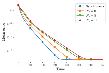
Figure 1: Error trajectories of the DOT-ADMM Algorithm with synchronous and asynchronous updates for different numbers of slow nodes.

Hereafter, unless otherwise stated we use the DOT-ADMM Algorithm with $\theta=10^{-8}$, for a local update time of ${\sim 2.42\times 10^{-3}s}$. For comparison, we note that a local update of DGT (with hand-tuned parameters to improve performance) requires $\sim 1.90\times 10^{-3}s$, and in the simulations we allow DGT to run two iterations per each iteration of the DOT-ADMM, to account for the longer time required in the latter local updates.

6.2 Quantized communications

As in the section above, we consider a static logistic regression problem, and assume that the agents can exchange quantized communications. In particular, an agent $i$ can only send the quantized version $q(x)$ of a message $x\in\mathbb{R}^{p}$, as defined component-wise by

$$[q(x)]_{j}=\begin{cases}\underline{q}&\text{if}\ [x]_{j}<\underline{q}\\ \delta\lfloor[x]_{j}/\delta\rfloor&\text{if}\ \underline{q}\leq[x]_{j}\leq\overline{q}\\ \overline{q}&\text{if}\ [x]_{j}>\overline{q}\\ \end{cases},\quad j\in\{1,\ldots,p\}$$

with $\overline{q}=-\underline{q}=10$, and $\delta>0$ the quantization level. Table 2 reports the asymptotic error of the DOT-ADMM for different quantization levels $\delta$.

Table 2: Asymptotic error for different quantization levels.

Quantization	Asymptotic error
No quantization	$5.30\times 10^{-8}$
$\delta=10^{-10}$	$5.30\times 10^{-8}$
$\delta=10^{-8}$	$7.36\times 10^{-8}$
$\delta=10^{-6}$	$4.74\times 10^{-6}$
$\delta=10^{-4}$	$5.64\times 10^{-4}$
$\delta=10^{-2}$	$5.32\times 10^{-2}$
$\delta=10^{-1}$	$4.91\times 10^{-1}$

6.3 Asynchrony

In Section 6.1 we discussed how the local updates (4) for a logistic regression problem need to be computed recursively as the proximal does not have a closed form solution. We then discussed how the threshold specifying the accuracy of the local update impacts the convergence of the algorithm. Here we consider how recursive local updates can lead to asynchronous operations of the agents, due to their heterogeneous computational capabilities.

We consider the following scenario: at iteration $k$ each agent completes the local update (4) – using $\theta=10^{-8}$ – with some probability, $\underline{p}$ or $\overline{p}$, $\underline{p}<\overline{p}$. The agents characterized by the smaller probability $\underline{p}$ are the “slow” nodes, which, having fewer computational resources, take on average a longer time to reach the threshold $\theta$. Notice that all the nodes use the same threshold, and their more or less frequent updates mimic the effect of different resources.

In Figure 1 we report the mean tracking error (as averaged over $100$ Monte Carlo iterations) for the asynchronous case with different numbers of slow nodes $N_{s}$. We also compare the result with the error in the synchronous case, in which all nodes complete an update at each iteration $k$. As discussed in Remark 2, asynchronous agent operations, which translate into random coordinate updates, lead to worse convergence rates. Indeed, the more frequent the updates are, the faster the convergence rate (until achieving that of the synchronous version), and the introduction of slower nodes implies less frequent coordinate updates overall.

6.4 Online optimization

In this section, we evaluate the performance of the DOT-ADMM Algorithm when applied to two instances of the online logistic regression problem, in which the local cost functions are piece-wise constant. Specifically, the costs change $10$ and $100$ times, respectively, and are generated so that the maximum distance between consecutive optima is $\sim 2.5$ (cf. Assumption 2). In Figure 2 we report the tracking error of DOT-ADMM when applied to the two problems. Notice that when the problem changes less frequently, the DOT-ADMM has time to converge to smaller errors, up to the bound imposed by the inexact local updates (computed with $\theta=10^{-4}$). Notice that in the transient the convergence is linear, as predicted by the theory. On the other hand, more frequent changes in the problem yield larger tracking errors overall.

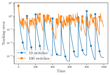
Figure 2: Tracking error of the DOT-ADMM Algorithm applied to two online problems with different piece-wise constant cost functions.

6.5 Comparison with gradient tracking methods

We conclude by comparing the DOT-ADMM Algorithm with two gradient tracking methods:

• ra-GD [24]: which makes use of the robust ratio consensus to ensure convergence in the presence of asynchrony,

• LEAD [49]: which is designed to be robust to a certain class of unbiased quantizers.

Due to the fact that DOT-ADMM requires a longer time to update the local states (cf. Section 6.1), ra-GD and LEAD were run for a larger number of iterations to match the computational time of DOT-ADMM.

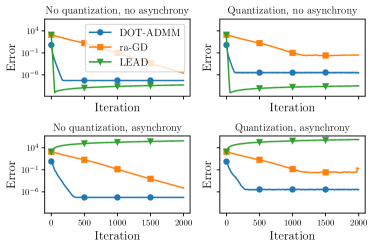
Figure 3: Comparison of the DOT-ADMM with [24, 49] for different scenarios combining quantization and asynchrony.

In Figure 3 we report the error for the three methods for different scenarios combining quantization and asynchrony. In particular, we either use or not the quantizer [49, eq. (14)], and the agents either activate synchronously or asynchronusly, using the same set-up as Section 6.3. In accordance with the theory, ra-GD is robust to asynchrony, although the convergence is somewhat slow due to a conservative step-size choice. On the other hand, when quantization is employed the algorithm seems to converge only to a neighborhood of the optimal solution, which is larger than the neighborhood reached by DOT-ADMM (despite the fact that DOT-ADMM also uses inexact updates). As predicted, LEAD shows convergence in the presence of quantization; however, the algorithm is not robust to asynchrony and seems to diverge when the agents are not synchronized. Overall, only the DOT-ADMM shows robustness to both asynchrony and quantization of the communications.

7 Conclusions

This paper proposes the DOT-ADMM Algorithm to solve online learning problems in a multi-agent setting under challenging network constraints, such as asynchronous and inexact agent computations, and unreliable communications. The convergence and robustness of the DOT-ADMM Algorithm have been proven by deriving novel theoretical results in stochastic operator theory for the class of metric-subregular operators, which turns out to be an important class of operators that shows linear convergence to the set of optimal solutions. The broad applicability of this class of operators is supported by the fact that the operator ruling the DOT-ADMM Algorithm applied to the standard linear and logistic regression problems is indeed metric subregular. Future works will focus on studying the optimal design of the DOT-ADMM algorithm and on the characterization of the linear rate of convergence for specific distributed problems, e.g. online learning and dynamic tracking.

References

- [1] Daniel K. Molzahn, Florian Dorfler, Henrik Sandberg, Steven H. Low, Sambuddha Chakrabarti, Ross Baldick and Javad Lavaei “A Survey of Distributed Optimization and Control Algorithms for Electric Power Systems” In IEEE Transactions on Smart Grid 8.6, 2017, pp. 2941–2962
- [2] Angelia Nedić and Ji Liu “Distributed Optimization for Control” In Annual Review of Control, Robotics, and Autonomous Systems 1.1, 2018, pp. 77–103
- [3] E. Montijano, G. Oliva and A. Gasparri “Distributed Estimation and Control of Node Centrality in Undirected Asymmetric Networks” In IEEE Transactions on Automatic Control 66.5, 2021, pp. 2304–2311
- [4] D. Deplano, M. Franceschelli and A. Giua “Dynamic Min and Max Consensus and Size Estimation of Anonymous Multiagent Networks” In IEEE Transactions on Automatic Control 68.1, 2023, pp. 202–213
- [5] Diego Deplano, Mauro Franceschelli and Alessandro Giua “A nonlinear Perron–Frobenius approach for stability and consensus of discrete-time multi-agent systems” In Automatica 118 Elsevier, 2020, pp. 109025
- [6] M. Santilli, M. Franceschelli and A. Gasparri “Dynamic Resilient Containment Control in Multirobot Systems” In IEEE Transactions on Robotics 38.1, 2022, pp. 57–70
- [7] D. Deplano, M. Franceschelli and A. Giua “Novel Stability Conditions for Nonlinear Monotone Systems and Consensus in Multi-Agent Networks” In IEEE Transactions on Automatic Control, 2023, pp. 1–14 DOI: 10.1109/TAC.2023.3246419
- [8] Y. Shang “Resilient consensus in multi–agent systems with state constraints” In Automatica 122, 2020, pp. 109288
- [9] Lina Sheng, Wei Gu, Ge Cao and Xiaogang Chen “A distributed detection mechanism and attack–resilient strategy for secure voltage control of AC microgrids” In CSEE Journal of Power and Energy Systems, 2022, pp. 1–10 DOI: 10.17775/CSEEJPES.2020.07140
- [10] Matteo Santilli, Mauro Franceschelli and Andrea Gasparri “Secure rendezvous and static containment in multi-agent systems with adversarial intruders” In Automatica 143 Elsevier, 2022, pp. 110456
- [11] Stephen Boyd, Neal Parikh, Eric Chu, Borja Peleato and Jonathan Eckstein “Distributed optimization and statistical learning via the alternating direction method of multipliers” In Foundations and Trends® in Machine learning 3.1 Now Publishers, Inc., 2011, pp. 1–122
- [12] Liangxin Qian, Ping Yang, Ming Xiao, Octavia A. Dobre, Marco Di Renzo, Jun Li, Zhu Han, Qin Yi and Jiarong Zhao “Distributed Learning for Wireless Communications: Methods, Applications and Challenges” In IEEE Journal of Selected Topics in Signal Processing 16.3, 2022, pp. 326–342
- [13] Jihong Park, Sumudu Samarakoon, Anis Elgabli, Joongheon Kim, Mehdi Bennis, Seong-Lyun Kim and Mérouane Debbah “Communication-Efficient and Distributed Learning Over Wireless Networks: Principles and Applications” In Proceedings of the IEEE 109.5, 2021, pp. 796–819
- [14] Giuseppe Notarstefano, Ivano Notarnicola and Andrea Camisa “Distributed Optimization for Smart Cyber-Physical Networks” In Foundations and Trends® in Systems and Control 7.3, 2019, pp. 253–383
- [15] Tao Yang, Xinlei Yi, Junfeng Wu, Ye Yuan, Di Wu, Ziyang Meng, Yiguang Hong, Hong Wang, Zongli Lin and Karl H. Johansson “A survey of distributed optimization” In Annual Reviews in Control 47, 2019, pp. 278–305
- [16] Tomer Gafni, Nir Shlezinger, Kobi Cohen, Yonina C. Eldar and H. Vincent Poor “Federated Learning: A signal processing perspective” In IEEE Signal Processing Magazine 39.3, 2022, pp. 14–41
- [17] Zhimin Peng, Tianyu Wu, Yangyang Xu, Ming Yan and Wotao Yin “Coordinate Friendly Structures, Algorithms and Applications” In Annals of Mathematical Sciences and Applications 1.1, 2016, pp. 57–119
- [18] Anastasia Koloskova, Nicolas Loizou, Sadra Boreiri, Martin Jaggi and Sebastian Stich “A Unified Theory of Decentralized SGD with Changing Topology and Local Updates” In Proceedings of the 37th International Conference on Machine Learning 119, Proceedings of Machine Learning Research PMLR, 2020, pp. 5381–5393
- [19] Neal Parikh and Stephen Boyd “Proximal Algorithms” In Foundations and Trends® in Optimization 1.3, 2014, pp. 127–239
- [20] R. Xin, S. Pu, A. Nedić and U. A. Khan “A General Framework for Decentralized Optimization With First-Order Methods” In Proceedings of the IEEE 108.11, 2020, pp. 1869–1889
- [21] K. Yuan, W. Xu and Q. Ling “Can Primal Methods Outperform Primal-Dual Methods in Decentralized Dynamic Optimization?” In IEEE Transactions on Signal Processing 68, 2020, pp. 4466–4480
- [22] Guido Carnevale, Francesco Farina, Ivano Notarnicola and Giuseppe Notarstefano “GTAdam: Gradient Tracking With Adaptive Momentum for Distributed Online Optimization” In IEEE Transactions on Control of Network Systems, 2023, pp. 1–12
- [23] Jinming Xu, Shanying Zhu, Yeng Chai Soh and Lihua Xie “Convergence of Asynchronous Distributed Gradient Methods Over Stochastic Networks” In IEEE Transactions on Automatic Control 63.2, 2018, pp. 434–448
- [24] Nicoletta Bof, Ruggero Carli, Giuseppe Notarstefano, Luca Schenato and Damiano Varagnolo “Multiagent Newton-Raphson Optimization Over Lossy Networks” In IEEE Transactions on Automatic Control 64.7, 2019, pp. 2983–2990
- [25] Y. Tian, Y. Sun and G. Scutari “Achieving Linear Convergence in Distributed Asynchronous Multiagent Optimization” In IEEE Transactions on Automatic Control 65.12, 2020, pp. 5264–5279
- [26] Huan Li, Zhouchen Lin and Yongchun Fang “Variance Reduced EXTRA and DIGing and Their Optimal Acceleration for Strongly Convex Decentralized Optimization” In Journal of Machine Learning Research 23.222, 2022, pp. 1–41
- [27] Jinlong Lei, Peng Yi, Jie Chen and Yiguang Hong “Distributed Variable Sample-Size Stochastic Optimization With Fixed Step-Sizes” In IEEE Transactions on Automatic Control 67.10, 2022, pp. 5630–5637
- [28] Michelangelo Bin, Ivano Notarnicola and Thomas Parisini “Stability, Linear Convergence, and Robustness of the Wang-Elia Algorithm for Distributed Consensus Optimization” In 2022 IEEE 61st Conference on Decision and Control (CDC) Cancun, Mexico: IEEE, 2022, pp. 1610–1615
- [29] Zhimin Peng, Yangyang Xu, Ming Yan and Wotao Yin “ARock: an Algorithmic Framework for Asynchronous Parallel Coordinate Updates” In SIAM Journal on Scientific Computing 38.5, 2016, pp. A2851–A2879
- [30] Ermin Wei and Asuman Ozdaglar “On the O(1/k) convergence of asynchronous distributed alternating Direction Method of Multipliers” In 2013 IEEE Global Conference on Signal and Information Processing, 2013, pp. 551–554
- [31] Tsung-Hui Chang, Mingyi Hong, Wei-Cheng Liao and Xiangfeng Wang “Asynchronous Distributed ADMM for Large-Scale Optimization- Part I: Algorithm and Convergence Analysis” In IEEE Transactions on Signal Processing 64.12, 2016, pp. 3118–3130
- [32] Layla Majzoobi, Vahid Shah-Mansouri and Farshad Lahouti “Analysis of distributed ADMM algorithm for consensus optimisation over lossy networks” In IET Signal Processing 12.6, 2018, pp. 786–794
- [33] N. Bastianello, R. Carli, L. Schenato and M. Todescato “Asynchronous Distributed Optimization over Lossy Networks via Relaxed ADMM: Stability and Linear Convergence” In IEEE Transactions on Automatic Control 66.6, 2021, pp. 2620–2635
- [34] Layla Majzoobi, Farshad Lahouti and Vahid Shah-Mansouri “Analysis of Distributed ADMM Algorithm for Consensus Optimization in Presence of Node Error” In IEEE Transactions on Signal Processing 67.7, 2019, pp. 1774–1784
- [35] Yue Xie and Uday V. Shanbhag “SI-ADMM: A Stochastic Inexact ADMM Framework for Stochastic Convex Programs” In IEEE Transactions on Automatic Control 65.6, 2020, pp. 2355–2370
- [36] Patrick L. Combettes and Jean-Christophe Pesquet “Stochastic Quasi-Fejér Block-Coordinate Fixed Point Iterations with Random Sweeping” In SIAM Journal on Optimization 25.2, 2015, pp. 1221–1248
- [37] Wei Shi, Qing Ling, Kun Yuan, Gang Wu and Wotao Yin “On the Linear Convergence of the ADMM in Decentralized Consensus Optimization” In IEEE Transactions on Signal Processing 62.7, 2014, pp. 1750–1761
- [38] F. Iutzeler, P. Bianchi, P. Ciblat and W. Hachem “Explicit Convergence Rate of a Distributed Alternating Direction Method of Multipliers” In IEEE Transactions on Automatic Control 61.4, 2016, pp. 892–904
- [39] Ali Makhdoumi and Asuman Ozdaglar “Convergence Rate of Distributed ADMM Over Networks” In IEEE Transactions on Automatic Control 62.10, 2017, pp. 5082–5095
- [40] Heinz H. Bauschke and Patrick L. Combettes “Convex Analysis and Monotone Operator Theory in Hilbert Spaces” In Convex Analysis and Monotone Operator Theory in Hilbert Spaces Cham, Switzerland: Springer, 2017
- [41] Emiliano Dall’Anese, Andrea Simonetto, Stephen Becker and Liam Madden “Optimization and Learning With Information Streams: Time-varying algorithms and applications” In IEEE Signal Processing Magazine 37.3, 2020, pp. 71–83
- [42] A. Simonetto, E. Dall’Anese, S. Paternain, G. Leus and G. B. Giannakis “Time-Varying Convex Optimization: Time-Structured Algorithms and Applications” In Proceedings of the IEEE 108.11, 2020, pp. 2032–2048
- [43] F. Bullo “Contraction Theory for Dynamical Systems” Kindle Direct Publishing, 2023 URL: https://fbullo.github.io/ctds
- [44] Nicola Bastianello, Liam Madden, Ruggero Carli and Emiliano Dall’Anese “A Stochastic Operator Framework for Optimization and Learning with Sub-Weibull Errors” In arXiv preprint arXiv:2105.09884, 2023
- [45] S. Sundhar Ram, A. Nedić and V. V. Veeravalli “Distributed Stochastic Subgradient Projection Algorithms for Convex Optimization” In Journal of Optimization Theory and Applications 147.3, 2010, pp. 516–545
- [46] Stephen M Robinson “Some continuity properties of polyhedral multifunctions” In Mathematical Programming at Oberwolfach Springer, 1981, pp. 206–214
- [47] A. Themelis and P. Patrinos “SuperMann: A Superlinearly Convergent Algorithm for Finding Fixed Points of Nonexpansive Operators” Cited By :14 In IEEE Transactions on Automatic Control 64.12, 2019, pp. 4875–4890 URL: www.scopus.com
- [48] Nicola Bastianello “tvopt: A Python Framework for Time-Varying Optimization” In 2021 60th IEEE Conference on Decision and Control (CDC), 2021, pp. 227–232
- [49] Xiaorui Liu, Yao Li, Rongrong Wang, Jiliang Tang and Ming Yan “Linear convergent decentralized optimization with compression” In arXiv preprint arXiv:2007.00232, 2020