Iterative, Small-Signal $\mathcal{L}_{2}$ Stability Analysis of Nonlinear Constrained Systems

Abstract

This paper provides a method to analyze the small-signal $\mathcal{L}_{2}$ gain of control-affine nonlinear systems on compact sets via iterative semi-definite programs. First, a continuous piecewise affine (CPA) storage function and the corresponding upper bound on the $\mathcal{L}_{2}$ gain are found on a bounded, compact set’s triangulation. Then, to ensure that the state does not escape this set, a CPA barrier function is found that is robust to small-signal inputs. Small-signal $\mathcal{L}_{2}$ stability then holds inside each sublevel set of the barrier function inside the set where the storage function was found. The bound on the inputs is also found while searching for a barrier function. The method’s effectiveness is shown in a numerical example.

[Duke]organization=Thomas Lord Department of Mechanical Engineering and Materials Science, Duke University,addressline=304 Research Drive, city=Durham, postcode=27708, state=NC, country=USA

Theorem 3 establishes criteria to bound the $\mathcal{L}_{2}$ gain of a nonlinear system on a robustly positive invariant subset of the state-space. It simultaneously identifies a bound on the input disturbance signal’s infinity norm to which the subset is robustly positive invariant.

Algorithms are proposed to evaluate the criteria of Theorem 3, relying only on repeated solution of well-posed, convex optimization problems.

The paper provides systematic means to evaluate the gain of constrained, nonlinear systems under a small-signal requirement.

An iterative method allows rigorous verification of the small-signal requirement.

1 Introduction

Considering a system as an input-output map between two normed vector spaces, the $\mathcal{L}_{2}$-gain bounds the norm of the input above in the energy sense as it passes through the system [1]. If it is finite, input-output stability is established in the sense of $\mathcal{L}_{2}$. The $\mathcal{L}_{2}$-gain analysis is important in evaluating the performance of stable systems in the presence of norm-bounded disturbances [2, 3], and in studying the stability of interconnected systems via Small-Gain Theorem [4], which underpins $\mathcal{H}_{\infty}$ robust control. This paper gives an iterative method to bound the $\mathcal{L}_{2}$-gain of nonlinear time-invariant maps in which both the control inputs and the states in the state space representation are constrained.

For stable, linear, time-invariant systems, the $\mathcal{L}_{2}$-gain is equivalent to the $\mathcal{H}_{\infty}$ norm of the corresponding transfer function due to Parseval’s Theorem [5, p. 51] and can be found using the Bounded Real Lemma [6]. The connection between frequency and time domains can be used to find tight bounds on $\mathcal{L}_{2}$-gain. This allowed an efficient bisection algorithm in [7, 8] improving the method of [9] that was purely based on frequency domain analysis. These works inspired future, more sophisticated methods of [10, 11, 12, 13, 14, 15].

For nonlinear systems, $\mathcal{L}_{2}$-gain analysis remains a challenge [16, 17, 18]. An upper-bound on $\mathcal{L}_{2}$-gain is typically sought and tight bounds are hard to establish [19]. Due to modeling or physical limitations, and safety considerations, the input-output mapping may not be defined for a subset of the input vector space or the states in the internal description may be restricted, constraining the input-output mapping. This further complicates $\mathcal{L}_{2}$-gain analysis, even for linear systems. That said, the Hamilton-Jacobi (HJ) and dissipativity inequalities can be used to analyze $\mathcal{L}_{2}$ gain for nonlinear systems; it is just challenging to establish the existence of a positive semi-definite storage function satisfying these inequalities. Additionally, one needs to make sure that for a subset of admissible inputs, the HJ inequality holds and that the state remains inside the set of admissible states. These requirements can be verified by using the small-signal definition of $\mathcal{L}_{2}$ stability while ensuring that the state remains close to the origin either by input-to-state stability of the mapping, reachability analysis, or asymptotic stability of the unforced system [20]. For polynomial systems, the search for appropriate, polynomial storage functions was tackled in [20]. However, there is no assurance that the storage functions must be polynomial, and for general nonlinear systems, finding a storage function that satisfies the HJ inequality is generally a non-convex, computationally challenging problem.

In this paper, the $\mathcal{L}_{2}$-gain analysis of constrained, time-invariant, nonlinear maps is conducted using an iterative method that seeks CPA storage functions on the triangulations of the set of admissible states. Triangulation refinement searches a rich class of possible storage functions. Moreover, imposing barrier-like conditions on a shell ensures that the state constraints are satisfied for a set of admissible inputs. Like many iterative convex overbounding procedures such as [21], a bound on the number of iterations cannot be established. However, each step requires only the solution of an SDP. For constrained, control-affine, nonlinear systems, the proposed method analyses small-signal $\mathcal{L}_{2}$-gain without resorting to non-convex optimization.

2 Preliminaries

Notation. The $p$-norm, where $p\in[0,\infty]$, of $u\in\mathbb{R}^{m}$ is denoted by $||u||_{p}$. When no subscript is used, it means any $p$-norm is allowed. The induced norm of a matrix $A$ will be denoted $||A||_{\infty}=\sup_{||v||_{\infty}=1}Av$. The normed space of functions $u:[0,\infty]\mapsto\mathbb{R}^{m}$ is denoted by $\mathcal{L}_{p}$ with the norm $||u||_{\mathcal{L}_{p}}=(\int_{0}^{\infty}||u(t)||^{p}dt)^{(1/p)}<\infty$ for $p\in[1,\infty)$ and $||u||_{\mathcal{L}_{\infty}}=\sup_{t\geq 0}||u(t)||<\infty$. When the subscript is omitted, it means any $p$ is allowed. Whenever the dimension of signals bears clarification, a superscript $m$ is added as $\mathcal{L}^{m}$. The extended space of $\mathcal{L}$, denoted $\mathcal{L}_{e}$, is defined as $\Set{u\mid u_{\tau}\in\mathcal{L},\;\forall\tau\in[0,\infty)}$, where $u_{\tau}$ is the truncation of $u$ defined as $u_{\tau}(t)=u(t)$ for $0\leq t\leq\tau$ and $0$ otherwise. The set of real-valued functions with $r$ times continuously differentiable partial derivatives over their domain is denoted by $\mathcal{C}^{r}$. The $i^{\textrm{th}}$ element of a vector $x$ is denoted by $x^{(i)}$. The preimage of a function $f$ with respect to a subset $\Omega$ of its codomain is defined by $f^{-1}(\Omega){=}\{x{\mid}f(x){\in}\Omega\}$. The transpose of $x{\in}\mathbb{R}^{n}$ is denoted by $x^{\intercal}$. The vector of ones in $\mathbb{R}^{n}$ is denoted by $1_{n}$.

The interior, boundary, and closure of $\Omega\in\mathbb{R}^{n}$ are denoted by $\Omega\degree$, $\partial\Omega$, and $\bar{\Omega}$, respectively. The set of all compact subsets $\Omega{\subset}\mathbb{R}^{n}$ satisfying i) $\Omega\degree$ is connected and contains the origin, and ii) $\Omega=\overline{\Omega\degree}$, is denoted by $\mathfrak{R}^{n}$.

This paper concerns $\mathcal{L}$ stability, which is defined next.

Definition 1 ($\mathcal{L}$ stability[4])

A mapping $\mathcal{G}:\mathcal{L}_{e}^{m}\mapsto\mathcal{L}_{e}^{q}$ is $\mathcal{L}$ finite-gain stable if there exist $\gamma_{1},\gamma_{2}\geq 0$ such that

$$||(\mathcal{G}u)_{\tau}||_{\mathcal{L}}\leq\gamma_{1}||u_{\tau}||_{\mathcal{L}}+\gamma_{2}$$ (1)

for all $u\in\mathcal{L}_{e}^{m}$ and $\tau\in[0,\infty)$.         

When a $\gamma_{1}\geq 0$ is found, the $\mathcal{L}$ gain of $\mathcal{G}$ is less than or equal to $\gamma_{1}$. Since $\mathcal{G}$ is a state-space model of a dynamic system in this paper, causality, $(\mathcal{G}u)_{\tau}=(\mathcal{G}u_{\tau})_{\tau}$ holds.

When inputs are constrained, Definition 1 is modified as follows to only allow a subset of the input space.

Definition 2 (Small-signal $\mathcal{L}$ stability[22, Def 5.2])

The mapping $\mathcal{G}:\mathcal{L}_{e}^{m}\mapsto\mathcal{L}_{e}^{q}$ is $\mathcal{L}$ small-signal finite-gain stable if there exists $r_{u}>0$ such that (1) is satisfied for all $u\in\mathcal{L}_{e}^{m}$ with $\sup_{0\leq t\leq\tau}||u(t)||\leq r_{u}$.         

We use CPA functions to search for a storage function. They are defined on triangulation, described next.

Definition 3 (Affine independence[23])

A set of vectors $\{x_{0},\ldots,x_{n}\}$ in $\mathbb{R}^{n}$ is called affinely independent if $x_{1}-x_{0},\ldots,x_{n}-x_{0}$ are linearly independent.         

Definition 4 ($n$-simplex [23])

An $n$-simplex is the convex combination of $n+1$ affinely independent vectors in $\mathbb{R}^{n}$, denoted $\sigma{=}\textrm{co}(\{x_{j}\}_{j=0}^{n})$, where $x_{j}$’s are called vertices.         

In this paper, simplex always refers to $n$-simplex. By abuse of notation, $\mathcal{T}$ will refer to both a collection of simplexes and the set of points in all the simplexes of the collection.

Definition 5 (Triangulation [23])

A set $\mathcal{T}\in\mathfrak{R}^{n}$ is called a triangulation if it is a finite collection of $m_{\mathcal{T}}$ simplexes, denoted $\mathcal{T}=\{\sigma_{i}\}_{i=1}^{m_{\mathcal{T}}}$, and the intersection of any two simplexes in $\mathcal{T}$ is either a face or the empty set.

The following two conventions are used throughout this paper for triangulations and their simplexes. Let $\mathcal{T}=\{\sigma_{i}\}_{i=1}^{n}$. Further, let $\{x_{i,j}\}_{j=0}^{n}$ be $\sigma_{i}$’s vertices, making $\sigma_{i}=\textrm{co}(\{x_{i,j}\}_{j=0}^{n})$. The choice of $x_{i,0}$ in $\sigma_{i}$ is arbitrary unless $0\in\sigma_{i}$, in which case $x_{i,0}=0$. The vertices of the triangulation $\mathcal{T}$ that are in $\Omega\subseteq\mathcal{T}$ is denoted by $\mathbb{E}_{\Omega}$.         

Lemma 1 (​​[23, Rem. 9])

Consider the triangulation $\mathcal{T}=\{\sigma_{i}\}_{i=1}^{m_{\mathcal{T}}}$, where $\sigma_{i}=\textrm{co}(\{x_{i,j}\}_{j=0}^{n})$, and a set $\mathbf{W}=\left\{W_{x}\right\}_{x\in\mathbb{E}_{\mathcal{T}}}\subset\mathbb{R}$. Let $X_{i}\in\mathbb{R}^{n\times n}$ be a matrix that has $x_{i,j}-x_{i,0}$ as its $j$-th row, and $\bar{W}_{i}{\in}\mathbb{R}^{n}$ be a vector that has $W_{x_{i,j}}{-}W_{x_{i,0}}$ as its $j$-th element. The function $W(x)=x^{\intercal}_{i}X^{-1}_{i}\bar{W}_{i}+\omega_{i}$ is the unique, CPA interpolation of W on $\mathcal{T}$, satisfying $W(x){=}W_{x}$, $\forall x{\in}\mathbb{E}_{\mathcal{T}}$.         

The Dini derivative of a CPA function $W$ at $x$ is

$$D^{+}W(x)=\textrm{lim\,sup}_{h\rightarrow 0^{+}}\nicefrac{{(W(x+hg(x))-W(x))}}{{h}},$$

which equals $\dot{W}(x)$ where $W\in\mathcal{C}^{1}$ [23]. Also, a continuous function $g(x)\in\mathbb{R}^{n}$ is piecewise $\mathcal{C}^{2}$ on a triangulation $\mathcal{T}=\{\sigma_{i}\}_{i=1}^{m_{\mathcal{T}}}$, denoted $g\in\mathcal{C}^{2}(\mathcal{T})$, if it is in $\mathcal{C}^{2}$ on $\sigma_{i}$ for all $i\in\mathbb{Z}_{1}^{m_{\mathcal{T}}}$ [24, Def. 5] [25]. The following lemma, which will be used frequently, overbounds a $\mathcal{C}^{2}$ vector function on a simplex.

Lemma 2 (​​[23, Thm. 1],[26, Prop. 2.2, Lem. 2.3])

Consider $\hat{\Omega}\in\mathfrak{R}^{n}$ and let $g:\hat{\Omega}\mapsto\mathbb{R}^{n}$ satisfy $g\in\mathcal{C}^{2}(\mathcal{T})$ for some triangulation, $\mathcal{T}=\{\sigma_{i}\}_{i=1}^{m_{\mathcal{T}}}$ of $\hat{\Omega}$. Then, for any $x\in\sigma_{i}=\textrm{co}(\{x_{i,j}\}_{j=0}^{n})\in\mathcal{T}$,

$$||g(x)-\sum_{j=0}^{n}\lambda_{j}g(x_{i,j})||_{\infty}\leq\underline{\beta}_{i}\sum_{j=0}^{n}\lambda_{j}c_{i,j},$$ (2)

where $\{\lambda_{j}\}_{j=0}^{n}\in\mathbb{R}$ is the set of unique coefficients satisfying $x=\sum_{j=0}^{n}\lambda_{j}x_{i,j}$ with $\sum_{j=0}^{n}\lambda_{j}=1$ and $0\leq\{\lambda_{j}\}_{j=0}^{n}\leq 1$, and

$$c_{i,j}{=} \frac{n}{2}||x_{i,j}{-}x_{i,0}||(\max_{k\in\mathbb{Z}_{1}^{n}}||x_{i,k}{-}x_{i,0}||{+}||x_{i,j}{-}x_{i,0}||),\textrm{ and}$$

$$\underline{\beta}_{i}\geq \max_{p,q,r\in\mathbb{Z}_{1}^{n}}\max_{\xi\in\sigma_{i}}\left|\left.\nicefrac{{\partial^{2}g(x)^{(p)}}}{{\partial x^{(q)}\partial x^{(r)}}}\right|_{x=\xi}\right|.$$

        

One of the key contributions of this work is performing gain analysis for constrained nonlinear systems. Barrier functions will be a key tool allowing us to identify under which inputs the states will remain feasible. The following definition modifies the zeroing barrier function proposed in [27] by allowing $W$ to have positive time derivatives inside $\mathcal{A}_{1}$, which means the decrease condition is not required everywhere in $\mathcal{A}$.

Definition 6

Consider the system $\dot{x}=g(x)$, $x\in\mathcal{X}\in\mathfrak{R}^{n}$, where $g:\mathcal{X}\mapsto\mathbb{R}^{n}$ is a Lipschitz map. Let $\hat{\Omega},\mathcal{A}_{1}\in\mathfrak{R}^{n}$ satisfy $\mathcal{A}_{1}\subset\hat{\Omega}$. Further, let $W:\hat{\Omega}\mapsto\mathbb{R}$ be a Lipschitz function satisfying

$$W(x) >0,\quad \forall x\in\Omega,$$ (3a)

$$D^{+}W(x) \leq-b_{2},\quad \forall x\in(\Omega\backslash\mathcal{A}_{1})\degree,$$ (3b)

with $b_{2}>0$. Let $\mathcal{A}$ be a sublevel set of $W$ for which $\mathcal{A}_{1}\subset\mathcal{A}\subseteq\hat{\Omega}$ holds. Then, the restriction of $W$ to $\mathcal{A}\degree$, that is $W:\mathcal{A}\degree\mapsto\mathbb{R}$ is a barrier function.         

3 Main Results

Gain is typically established using HJ inequalities, like those found in [16, Thm 2], but these theorems typically apply over $\mathbb{R}^{n}$ We will show that small-signal finite-gain $\mathcal{L}_{2}$ stability can be ensured similarly if the state remains in a neighborhood of the origin for all $t\geq 0$.

We formulate the search for a CPA function $V$ establishing such an HJ inequality to ensure small-signal finite-gain $\mathcal{L}_{2}$ stability of constrained nonlinear systems. Exploiting the structure of CPA functions, we put Lyapunov-like properties on a shell inside a triangulation to find a positive-invariant set. This works much like a control barrier function that ensures states remain in a feasible region, but is robust to bounded input disturbances and does not impose convergence to an equilibrium. Moreover, we characterize the set of inputs for which the small-gain properties hold. The theorems in this section formulate this search. The first one seeks a CPA storage function $V$ to verify (11) on a bounded set.

Theorem 1

Consider the constrained mapping $\mathcal{G}:\mathcal{L}^{m}_{e}\mapsto\mathcal{L}^{q}_{e}$ defined by $y=\mathcal{G}u$ and

$$\dot{x}=f(x)+G(x)u,\;x\in\mathcal{X}\in\mathfrak{R}^{n},\;u\in\mathcal{U}\in\mathfrak{R}^{m},$$ (4)

$$y=h(x),\ \forall t\in[0,\infty)$$

where $f(0)=0$, $h(0)=0$, and $\bar{g}(0)=0$ for $\bar{g}(x)=||G(x)G^{\intercal}(x)||_{\infty}$. Suppose that $f,G,h\in\mathcal{C}^{2}(\mathcal{T})$ for a triangulation, $\mathcal{T}=\{\sigma_{i}\}_{i=1}^{m_{\mathcal{T}}}$, of a set $\Omega\in\mathfrak{R}^{n}$. There exist $\mathbf{V}=\{V_{x}\}_{x\in\mathbb{E}_{\mathcal{T}}}\subset\mathbb{R}$, $\mathbf{L}=\{l_{i}\}_{i=1}^{m_{\mathcal{T}}}\subset\mathbb{R}^{n}$, and $b_{1},\gamma\in\mathbb{R}$ satisfying

$$\gamma>0,\;$$ (5a)

$$V_{x}\geq 0,\; \forall x\in\mathbb{E}_{\mathcal{T}},$$ (5b)

$$|{\nabla V}_{i}|\leq l_{i}, \forall i\in\mathbb{Z}_{1}^{m_{\mathcal{T}}},$$ (5c)

$$H_{i,j}\leq-b_{1},\;\; \forall i\in\mathbb{Z}_{1}^{m_{\mathcal{T}}},\;\forall j\in\mathbb{Z}_{0}^{n},\;x\neq 0$$ (5d)

where

$$\!\!\!H_{i,j}= f(x_{i,j})^{\intercal}{\nabla V}_{i}+0.5||h(x_{i,j})||_{2}^{2}+(1_{n}^{\intercal}l_{i}\beta_{i}+0.5\tilde{\beta_{i}})c_{i,j}$$

$$+\frac{1}{2\gamma}(\bar{g}(x_{i,j})+\bar{\beta}_{i}c_{i,j})(1_{n}^{\intercal}l_{i})^{2}$$ (6)

$$c_{i,j}{=} \frac{n}{2}||x_{i,j}{-}x_{i,0}||(\max_{k\in\mathbb{Z}_{1}^{n}}||x_{i,k}{-}x_{i,0}||{+}||x_{i,j}{-}x_{i,0}||),$$ (7)

$$\beta_{i}\geq \max_{p,q,r\in\mathbb{Z}_{1}^{n}}\max_{\xi\in\sigma_{i}}\left|\left.\nicefrac{{\partial^{2}f(x)^{(p)}}}{{\partial x^{(q)}\partial x^{(r)}}}\right|_{x=\xi}\right|,$$ (8)

$$\tilde{\beta}_{i}\geq \max_{q,r\in\mathbb{Z}_{1}^{n}}\max_{\xi\in\sigma_{i}}\left|\left.\nicefrac{{\partial^{2}h^{\intercal}(x)h(x)}}{{\partial x^{(q)}\partial x^{(r)}}}\right|_{x=\xi}\right|,\text{ and}$$ (9)

$$\bar{\beta}_{i}\geq \max_{q,r\in\mathbb{Z}_{1}^{n}}\max_{\xi\in\sigma_{i}}\left|\left.\nicefrac{{\partial^{2}||\bar{g}(x)||_{\infty}}}{{\partial x^{(q)}\partial x^{(r)}}}\right|_{x=\xi}\right|.$$ (10)

If further $b_{1}>0$, then the HJ inequality,

$$\!\!\!\!\hat{H}\triangleq\nabla{V}^{\intercal}f(x)+\frac{1}{2\gamma}||G^{\intercal}(x)\nabla{V}||_{2}^{2}+\frac{1}{2}||h(x)||_{2}^{2}\leq 0,$$ (11)

is satisfied for all $x\in\Omega\degree$.         

Proof 1

To see that (5) is feasible, observe that for any $\gamma$ and $V_{x}$ satisfying (5a)-(5b), Lemma 1 can be used to compute $l_{i}=|\nabla{V}_{i}|$, verifying (5c).

Each $c_{i,j}$ is finite because $\Omega\in\mathfrak{R}^{n}$ implies $\mathcal{T}$ is bounded. Finite $H_{i,j},\,\beta_{i},\,\tilde{\beta}_{i}$,  $\bar{\beta}_{i}$, and consequently $b_{1}$, can be found because $f,G,h\in\mathcal{C}^{2}(\mathcal{T})$.

To show that (5) with $b_{1}>0$ implies (11) on $\Omega\degree$, we begin bounding each term in (11) using Lemma 2. This is possible because for any $x\in\Omega\degree$, there is a simplex, $\sigma_{i}=\textrm{co}(\{x_{i,j}\}_{j=0}^{n})$, such that $x=\sum_{j=0}^{n}\lambda_{j}x_{i,j}$, $0\leq\{\lambda_{i}\}_{i=0}^{n}\leq 1$, and $\sum_{j=0}^{n}\lambda_{j}=1$.

The first term’s bound in (11) was established in [23, Thm. 1], and is reproduced here for completeness. Combining the fact that $\nabla{V}^{\intercal}f(x)=\nabla{V}_{i}^{\intercal}f(x)$ on $\sigma_{i}$, Hölder’s inequality, (5c), (8), and Lemma 2 yields

$$\nabla {V}^{\intercal}f(x)=\nabla{V}_{i}^{\intercal}\left(\sum_{j=0}^{n}\lambda_{j}f(x_{i,j})+f(x)-\sum_{j=0}^{n}\lambda_{j}f(x_{i,j})\right)$$

$$\leq \sum_{j=0}^{n}\lambda_{j}\nabla{V}_{i}^{\intercal}f(x_{i,j})+||\nabla{V}_{i}||_{1}||f(x)-\sum_{j=0}^{n}\lambda_{j}f(x_{i,j})||_{\infty}$$

$$\leq \sum_{j=0}^{n}\lambda_{j}\nabla{V}_{i}^{\intercal}f(x_{i,j})+\beta_{i}1_{n}^{\intercal}l_{i}\sum_{j=0}^{n}\lambda_{j}c_{i,j}.$$ (12)

The second term of (11) will now be re-formulated so it can be bounded in union with the rest. For $x\in\sigma_{i}$, applying Hölder’s inequality, submultiplicativity of norms, the fact that $||v||_{\infty}\leq||v||_{1}$ for any $v\in\mathbb{R}^{n}$, and (5c) then show that

$$|| G^{\intercal}(x)\nabla{V}||_{2}^{2}\leq||\nabla{V}_{i}||_{1}||G(x)G^{\intercal}(x)\nabla{V}_{i}||_{\infty}$$ (13)

$$\leq||\nabla{V}_{i}||_{1}\bar{g}(x)||\nabla{V}_{i}||_{\infty}\leq||\nabla{V}_{i}||_{1}^{2}\bar{g}(x)\leq(1_{n}^{\intercal}l_{i})^{2}\bar{g}(x).$$

Note that $\bar{g}(x)$ and $\bar{h}(x)\triangleq h^{\intercal}(x)h(x)$, the third term in (11), are non-negative scalar functions. Using Lemma 2 once with $g(x)=\bar{g}(x)$ and again with $g(x)=\bar{h}(x)$ together with the fact that $||v||_{\infty}=|v|\;\forall v\in\mathbb{R}$ yields

$$\frac{1}{2\gamma}\bar{g}(x) \leq\sum_{j=0}^{n}\frac{1}{2\gamma}\left(\lambda_{j}\bar{g}(x_{i,j})+\bar{\beta}_{i}\lambda_{j}c_{i,j}\right)\text{, and}$$ (14)

$$\bar{h}(x) \leq\sum_{j=0}^{n}\left(\lambda_{j}\bar{h}(x_{i,j})+\tilde{\beta}_{i}\lambda_{j}c_{i,j}\right).$$ (15)

The upper bound on (11) can now be obtained. Summing (12), (14), and (15) reveals that $\hat{H}(x)\leq\sum_{j=0}^{n}\lambda_{j}H_{i,j}$, with $H_{i,j}$ given by (6). Finally, using (5d) on $\sigma_{i}$ and the facts that $0\leq\{\lambda_{i}\}_{i=0}^{n}\leq 1$ and $\sum_{j=0}^{n}\lambda_{j}=1$ yields

$$\hat{H}(x)\leq\sum_{j=0}^{n}\lambda_{j}H_{i,j}\leq-b_{1}\sum_{j=0}^{n}\lambda_{j}=-b_{1}.$$ (16)

Therefore, with $b_{1}>0$, (11) is verified at any $x\in\Omega\degree\setminus\{0\}.$ This also holds for $x=0$ because $f(0)=h(0)=\bar{g}(0)=0$ by assumption, $c_{i,0}=0$ by construction, and $x_{i,0}=0$ if $0\in\sigma_{i}$. Hence, $H_{i,0}=0$, verifying (11) for all $x\in\Omega\degree$.

In practice, even if $b_{1}>0$ is sought to satisfy Theorem 1 on $\Omega$, there might be a sub-triangulation of $\Omega$ on which $H_{i,j}$ is negative at all its vertices. The sub-triangulated region constitutes a set where Theorem 1 is satisfied.

Note that Theorem 1 satisfies (11) only on a subset of $\mathbb{R}^{n}$ because otherwise, (5) would have an infinite number of constraints. We will use small-signal properties to make sure that the state does not escape that subset. To do so, we search for a CPA barrier function separately by verifying the conditions of the following theorem.

Theorem 2

Consider the system

$$\dot{x}=f(x)+G(x)u,\;x\in\hat{\Omega}\in\mathfrak{R}^{n},$$ (17)

$$u=\kappa(t),\ \forall t\in[0,\infty)$$

where $f(0)$.

Let $\mathcal{T}=\{\sigma_{i}\}_{i=1}^{m_{\mathcal{T}}}$ be a triangulation of $\hat{\Omega}$. There exist $\mathbf{W}=\{W_{x}\}_{x\in\mathbb{E}_{\mathcal{T}}}\subset\mathbb{R}$, $\hat{\mathbf{L}}=\{\hat{l}_{i}\}_{i=1}^{m_{\mathcal{T}}}\subset\mathbb{R}^{n}$, and $b_{2},\hat{u}\in\mathbb{R}$ satisfying

$$\hat{u}> 0,$$ (18a)

$$W_{x}> 0,\ \forall x\in\mathbb{E}_{\mathcal{T}},$$ (18b)

$$||{\nabla W}_{i}||_{1}\leq \hat{l}_{i},\ \forall i\in\mathbb{Z}_{1}^{m_{\mathcal{T}}},$$ (18c)

$$D^{+}_{i,j}W\leq -b_{2},\ \forall i\in\mathbb{I}_{1},\ \forall j\in\mathbb{Z}_{0}^{n},$$ (18d)

where $D^{+}_{i,j}W=f(x_{i,j})^{\intercal}{\nabla W}_{i}+(1_{n}^{\intercal}\hat{l}_{i})(\beta_{i}c_{i,j}+\hat{g}_{i}\hat{u})$, $\hat{g}_{i}=\max_{x\in\sigma_{i}}||G(x)||_{\infty}$, $c_{i,j}$ is given in (7), and $\beta_{i}$ is given in (8). Suppose further that $b_{2}>0$ and there exists a sublevel set of $W(x)$, $\mathcal{A}\subseteq\hat{\Omega}$, and a second set, $\mathcal{A}_{1}\in\mathfrak{R}^{n}$, such that $\mathcal{A}_{1}\subset\mathcal{A}$ and $\partial\mathcal{A}_{1}\subseteq\{\partial\sigma_{i}\}_{i=1}^{m_{\mathcal{T}}}$. Then, the restriction of $W(x)$ to $\mathcal{A}\degree$, $W:\mathcal{A}\degree\mapsto\mathbb{R}$, is a barrier function provided $||\kappa(t)||_{\infty}\leq\hat{u}$ for $t\geq 0$.         

Proof 2

This proof parallels that of Theorem 1. The feasibility argument is nearly unchanged, so we focus on showing that (18) with $b_{2}>0$ satisfies Definition 6.

Since $W$ is CPA, (18b) implies (3a). For any $x\in(\hat{\Omega}\backslash\mathcal{A}_{1})\degree$, there is a simplex $\sigma_{i}=\textrm{co}(\{x_{i,j}\}_{j=0}^{n})\subseteq\mathcal{A}_{1}$ satisfying $x=\sum_{j=0}^{n}\lambda_{j}x_{i,j}$ for $0\leq\{\lambda_{i}\}_{i=0}^{n}\leq 1$ and $\sum_{j=0}^{n}\lambda_{j}=1$. On this simplex, (18c) and (18d) imply that $\nabla{W}^{\intercal}{f(x)}\leq\sum_{j=0}^{n}\lambda_{j}(\nabla{W}^{\intercal}f(x)+1_{n}^{\intercal}\hat{l}_{i}\beta_{i}c_{i,j})$ following arguments similar to those that established a bound on $\nabla{V}^{\intercal}f(x)$ in Theorem 1’s proof. Moreover, $\nabla{W}^{\intercal}G(x)u=\nabla{W}^{\intercal}_{i}G(x)u$ on $\sigma_{i}$. By Hölder’s inequality $\nabla{W}^{\intercal}_{i}G(x)u\leq||\nabla{W}_{i}||_{1}||G(x)u||_{\infty}$. Submultiplicativity of norms, (18c), and the definitions of $\hat{g}_{i}$ and $\hat{u}$ imply $\nabla{W}^{\intercal}_{i}G(x)u\leq 1_{n}^{\intercal}\hat{l}_{i}\hat{g}_{i}\hat{u}$. Adding the two derived inequalities, we have that $D^{+}W(x)=\nabla{W}^{\intercal}\dot{x}=D^{+}_{i,j}W\leq-b_{2}$, which verifies (3b).

Note that even if $b_{2}>0$ does not exist everywhere in $\mathcal{T}$, there might be a sub-triangulation containing $\mathcal{A}_{1}$ on which $D^{+}_{i,j}W$ is negative at all its vertices that are not in $\mathcal{A}_{1}\degree$. The restriction of $W$ to this sub-triangulation can be considered as the sought barrier function, but on the sub-triangulation, rather than $\hat{\Omega}$.

Using CPA functions $V$ and $W$, we can state the conditions for small-signal finite-gain $\mathcal{L}_{2}$ stability.

Theorem 3

Suppose that Theorems 1 and 2 both hold and $\mathcal{A}\subseteq\Omega$. Then, (4) is small-signal finite-gain $\mathcal{L}_{2}$ stable in $\mathcal{A}\degree$ for all $u\in\mathcal{L}_{e}^{m}$ with

$$\sup_{0\leq t\leq\tau}||u(t)||_{\infty}\leq\hat{u}$$

and the $\mathcal{L}_{2}$ gain is less than or equal to $\sqrt{\gamma}$.         

Proof 3

Note that $\mathcal{A}$ is a sub-level set of W, which is a barrier function that is robust to inputs $||u(t)||_{\infty}\leq\hat{u},\;\forall t\geq 0$. Positive-invariance of $\mathcal{A}\degree$ follows as a special case of [28, Thm 2.6] because $b_{2}$ is a positive number and $\mathcal{A},\mathcal{A}_{1}\in\mathfrak{R}^{n}$ in Theorem 2.

To bound the small-signal $\mathcal{L}_{2}-$gain, we must demonstrate that if $x(0)\in\mathcal{A}\degree$ and $||u(t)||_{\infty}\leq\hat{u}$, then (1) holds. Considering (4), $\dot{V}=\nabla{V}^{\intercal}(f(x)+G(x)u)$. By completing squares for the $\nabla{V}^{\intercal}G(x)u$ term using the two vectors $\sqrt{\gamma}u$ and $(1/\sqrt{\gamma})G(x)^{\intercal}\nabla{V}$ for $\gamma>0$, we have

$$\dot{V}= \nabla{V}^{\intercal}f(x)+\frac{1}{2}\gamma||u||_{2}^{2}+\frac{1}{2\gamma}||G(x)^{\intercal}\nabla{V}||_{2}^{2}$$

$$-\frac{\gamma}{2}||u-\frac{1}{\gamma}\nabla{V}^{\intercal}G(x)||_{2}^{2}.$$ (19)

Since $x(t)\in\mathcal{A}\degree\subseteq\Omega$, (11) can be substituted into (3) as

$$\dot{V}\leq-\frac{1}{2}||y||_{2}^{2}+\frac{1}{2}\gamma||u||_{2}^{2}-\frac{\gamma}{2}||u-\frac{1}{\gamma}\nabla{V}^{\intercal}G(x)||_{2}^{2}.$$

This means $||y||_{2}^{2}\leq\gamma||u||_{2}^{2}-2\dot{V}$. Integrating both sides and considering that $V(x)\geq 0$ on $\Omega$, we obtain

$$\int_{0}^{\tau}||y||_{2}^{2}dt\leq\gamma\int_{0}^{\tau}||u||_{2}^{2}dt+2V(x(0)).$$

Finally, taking square roots and applying the triangle inequality yields

$$||y_{\tau}||_{\mathcal{L}_{2}}\leq\sqrt{\gamma}||u_{\tau}||_{\mathcal{L}_{2}}+\sqrt{2V(x(0))},$$

which verifies (1).

Note that the three important characteristics of the system, namely $\gamma$, $\hat{u}$, and $\mathcal{A}$, found by Theorem 3 all depend on the choices for the triangulations and Hessian term’s upper bounds used in Theorems 1 and 2. For instance, $\gamma$ is only an upper bound on the system’s gain. Moreover, even if $\Omega$ in Theorem 1 and $\hat{\Omega}$ are the same, their corresponding triangulations do not have to be the same since (5) and (18) are solved independently.

4 Efficient Algorithms

While Theorem 3 presents sufficient conditions for finite-gain stability, it imposes non-convex constraints. This section proposes conservative, but convex, relaxations of the theorems, replacing them with iterative SDPs. The following theorems formulate each iteration.

4.1 Iterative SDPs for Theorem 1

While it is easy to obtain a feasible point of (5), only feasible points with $b_{1}>0$ are of use and the tightest possible gain bound is desirable. Minimizing $-b_{1}$ subject to (5) constitutes a search for an appropriate point, but it is a non-convex problem. Once $b_{1}>0$, minimizing $\gamma$ subject to (5) constitutes a search for the tightest possible gain bound, but it is a non-convex problem too. Here, we establish more conservative, but convex, criteria to impose (5), facilitating the required searches. Like most non-convex problems, it is unclear a priori where to begin searching, so two initialization heuristics are proposed.

Initialization 1

Assign $\gamma>0$ and $V_{x}\geq 0$ for all $x\in\mathbb{E}_{\mathcal{T}}$ to satisfy (5a) and (5b). Compute $l_{i}=|\nabla{V}_{i}|$ or all $i\in\mathbb{Z}_{1}^{m_{\mathcal{T}}}$ using Lemma 1. This verifies (5c). Using the computed values, find $b_{1}\in\mathbb{R}$ by calculating $\min-b_{1}$ subject to (5d) on all simplexes.

Initialization 2

Linearize (4) around the origin. Find $\gamma$ and the storage function, $V$, using KYP Lemma. Sample that function on the vertices to find $V_{x}$ satisfying (5b). Compute $l_{i}=|\nabla{V}_{i}|$ or all $i\in\mathbb{Z}_{1}^{m_{\mathcal{T}}}$ using Lemma 1. Assign $\gamma>0$ to satisfy (5a). Using the computed values, find $b_{1}\in\mathbb{R}$ by calculating $\min-b_{1}$ subject to (5d) on all simplexes.

Starting with any feasible point of (5), the following theorem establishes that a convex cost function can be iteratively minimized subject to an overbound of (5) through a series of SDPs. Towards verifying Theorem 1, $b_{1}>0$ can be sought by setting the cost function to $J(\mathbf{y})=-b_{1}$. Once a feasible point has been found with $b_{1}>0$, the constraints of Theorem 4 can be augmented with $b_{1}>0$ and a new objective can be chosen. In particular, selecting $J(\mathbf{y})=\gamma$ seeks the tightest possible gain bound.

Theorem 4

Consider (5) and let $\underline{\mathbf{y}}=[\underline{\mathbf{V}},\underline{\mathbf{L}},\underline{b}_{1},\underline{\gamma}]$ satisfy (5). Consider the following optimization.

$$\mathbf{y}^{\ast}=\operatorname*{argmin}_{\delta\mathbf{y}=[\delta\mathbf{V},\,\delta\mathbf{L},\delta b_{1},\,\delta\gamma]}\;\; J(\underline{\mathbf{y}}+\delta\mathbf{y})$$

s.t.

$$\gamma+\delta\gamma>0,\;$$ (20a)

$$V_{x}+\delta V_{x}\geq 0,\; \forall x\in\mathbb{E}_{\mathcal{T}},$$ (20b)

$$|\nabla{V}_{i}+\delta\nabla{V}_{i}|\leq l_{i}+\delta l_{i},\; \forall i\in\mathbb{Z}_{1}^{m_{\mathcal{T}}},$$ (20c)

$$P_{i,j}\preceq 0,\;\; \forall i\in\mathbb{Z}_{1}^{m_{\mathcal{T}}},\;j\in\mathbb{Z}_{0}^{n},\;x\neq 0$$ (20d)

where $\delta\nabla{V}_{i}$ in (20c) equals $X_{i}^{-1}\delta\bar{V}_{i}$ as in Lemma 1, and

$$P_{i,j}=\begin{bmatrix}\phi_{i,j}+b_{1}+\delta b_{1}&&\ast\\ \sqrt{e_{i,j}}1_{n}^{\intercal}(l_{i}+\delta l_{i})&&-(\gamma+\delta\gamma)\end{bmatrix},$$ (21)

with $\phi_{i,j}=f(x_{i,j})^{\intercal}(\nabla{V}_{i}+\delta\nabla{V}_{i})+1_{n}^{\intercal}(l_{i}+\delta l_{i})\beta_{i}c_{i,j}+\frac{1}{2}h^{\intercal}(x_{i,j})h(x_{i,j})+\frac{1}{2}\tilde{\beta}_{i}c_{i,j}$, and $e_{i,j}=\frac{\norm{G(x_{i,j})G^{\intercal}(x_{i,j})}_{\infty}}{2}$. Then $\underline{\mathbf{y}}+\delta\mathbf{y}$ is a feasible point for (5), and $J(\underline{\mathbf{y}}+\delta\mathbf{y})\leq J(\mathbf{y})$.

Proof 4

To see (20)’s feasibility, observe that $\delta\mathbf{y}{=}0$ satisfies (20) since in this case, (20) is equivalent to (5) with $\mathbf{y}{:=}\underline{\mathbf{y}}$. Substitution reveals that (20a)–(20d) imply (5a)–(5d) for $\mathbf{y}{=}\underline{\mathbf{y}}{+}\delta\mathbf{y}$. Note that (20d) is implied by Schur Complement[29, Ch 2]. Finally, $J(\underline{\mathbf{y}}{+}\delta\mathbf{y}){\leq}J(\mathbf{y})$ because otherwise $\delta\mathbf{y}{=}0$ would be a better, feasible solution.

4.2 Iterative SDPs for Theorem 2

Having a feasible point of (18), a cost function can be minimized while imposing a more conservative version of (18) iteratively through a series of SDPs. This approach requires a feasible point of (18). Two methods for obtaining such a point are given next.

Initialization 3

Assign $\hat{u}>0$ and $W_{x}\leq 0$ for all $x\in\mathbb{E}_{\mathcal{T}}$ to satisfy (18a) and (18b). Compute $\hat{l}_{i}=|\nabla{W}_{i}|$ or all $i\in\mathbb{Z}_{1}^{m_{\mathcal{T}}}$ using Lemma 1. This verifies (18c). Using the computed values, find $b_{2}\in\mathbb{R}$ by calculating $\min-b_{2}$ subject to (18d) on all simplexes.

Initialization 4

Linearize (4) around the origin. Design an LQR controller and find its corresponding quadratic Lyapunov function. Sample that function on the vertices to find $W_{x}$ satisfying (18b). Compute $\hat{l_{i}}=|\nabla{W}_{i}|$ or all $i\in\mathbb{Z}_{1}^{m_{\mathcal{T}}}$ using Lemma 1. Assign $\hat{u}>0$ to satisfy (18a). Using the computed values, find $b_{2}\in\mathbb{R}$ by calculating $\min-b_{2}$ subject to (18d) on all simplexes.

The following theorem formulates each step of the iterative improvement of the cost function in (18) as an SDP.

Theorem 5

Suppose that $\mathbf{y}=[\mathbf{W},\;\hat{\mathbf{L}},\;b_{2},\;\hat{u}]$ is a feasible point for (18). Consider the following optimization

$$\mathbf{y}^{\ast} =\operatorname*{argmin}_{\delta\mathbf{y}=[\delta\mathbf{W},\;\delta\hat{\mathbf{L}},\;\delta b_{2},\;\delta\hat{u}]}\;\; J(\mathbf{y}+\delta\mathbf{y})$$

s.t. $$\hat{u}+\delta\hat{u}>0,\;$$ (22a)

$$W_{x}+\delta W_{x}>0,\; \forall x\in\mathbb{E}_{\mathcal{T}},$$ (22b)

$$|{\nabla W}_{i}+\delta{\nabla W}_{i}|\leq\hat{l}_{i}+\delta\hat{l}_{i}, \forall i\in\mathbb{Z}_{1}^{m_{\mathcal{T}}},$$ (22c)

$$Q_{i,j}\preceq 0,\;\; \forall i\in\mathbb{I}_{1},\;\forall j\in\mathbb{Z}_{0}^{n},$$ (22d)

where $\delta\nabla{V}_{i}$ in (22c) equals $X_{i}^{-1}\delta\bar{V}_{i}$ as in Lemma 1, and

$$Q_{i,j}=\begin{bmatrix}\varphi_{i,j}+b_{2}+\delta b_{2}&&\ast&&\ast\\ 1_{n}^{\intercal}\delta\hat{l}_{i}&&-2&&\ast\\ \hat{g}_{i}\delta\hat{u}&&0&&-2\end{bmatrix},$$ (23)

with $\varphi_{i,j}=f(x_{i,j})^{\intercal}(\nabla{W}_{i}+\delta\nabla{W}_{i})+1_{n}^{\intercal}(l_{i}+\delta l_{i})(\beta_{i}c_{i,j}+\hat{g}_{i}\hat{u})+1_{n}^{\intercal}\hat{l}_{i}\hat{g}_{i}\delta\hat{u}$. Then $\underline{\mathbf{y}}+\delta\mathbf{y}$ is a feasible point for (5), and $J(\underline{\mathbf{y}}+\delta\mathbf{y})\leq J(\mathbf{y})$.

Proof 5

The proof follows similar to that of Theorem 1’s. To see that (22d) implies (18d), note that $u^{\intercal}v{\leq}0.5(u^{\intercal}u{+}v^{\intercal}v)$ for any vectors $u,v$ with the same dimension. Applying this fact and using Schur Complement, (22d) is obtained.

Note that $b_{1},b_{2}>0$ are needed in Theorems 1 and 2. However, the feasible initializations we provided for them don’t guarantee that. Moreover, the smallest value for the system gain and largest $\hat{u}$ are sought.

So, we use $J=-b_{1}$ and $J=-b_{2}$ in Theorems 20 and 22, respectively, to iteratively increase their initial values until $b_{1},b_{2}>0$ are found. Moreover, since the smallest gain is sought for a system, the iterative search for smaller $\gamma$ can be pursued by $J=\gamma$ while keeping $b_{1}>0$ in Theorem 4. Similarly, the largest $\hat{u}$ is sought for the system. So, $J=-\hat{u}$ can be used to achieve it iteratively while keeping $b_{2}>0$ in Theorem 5. Algorithm 1 gives the discussed strategy. Given $\Omega\in\mathfrak{R}^{n}$ and its triangulation, it tries to find $b_{1}>0$ using a sequence of SDPs initialized by Initialization 1 or 2 and using Theorem 4 repeatedly. If successful, it proceeds to minimize $\gamma$ while keeping $b_{1}$ positive. At this point, a storage function and an upper bound on the system’s gain are found on $\Omega$. Next, given $\hat{\Omega}\in\mathfrak{R}^{n}$ and its triangulation, it tries to find $b_{2}>0$ using a sequence of SDPs initialized by Initialization 3 or 4 and using Theorem 5 repeatedly. If successful, it proceeds to maximize $\hat{u}$ while keeping $b_{2}$ positive. Finally, using Theoerem 3, it returns $\gamma$, $\hat{u}$, and $\mathcal{A}$, which is the set on which small-signal finite-gain $\mathcal{L}_{2}$ stability holds. Note that if $b_{1}$ ($b_{2}$) is negative at line 6 (line 11), a positive $\hat{b}_{1}$ ($\hat{b}_{2}$) can be sought on a sub-triangulation.

Algorithm 1 $\mathcal{L}_{2}$-Stability Analysis

1:System (4), the sets $\Omega,\hat{\Omega},\mathcal{A}_{1}\in\mathfrak{R}^{n}$ and their triangulations

2:$\gamma$, $\hat{u}$, and $\mathcal{A}$

3:Find a feasible $\mathbf{y}$ satisfying Theorem 1 using Initialization 1 or 2

4:Let $J=-b_{1}$ in Theorem 4

5:repeat

6:     Solve (20)

7:until  $b_{1}>0$ is found

8:Add the constraint $b_{1}+\delta b_{1}>0$ to (20) $\triangleright$ To keep $b_{1}$ positive

9:Let $J=\gamma$ in Theorem 4 $\triangleright$ To minimize $\gamma$

10:repeat

11:     Solve (22)

12:until  $\gamma$ is not decreasing anymore $\triangleright$ At this point, a storage function and an upper bound on the system’s gain, $\gamma$, are found on $\Omega$

13:Find a feasible $\mathbf{y}$ satisfying Theorem 2 using Initialization 3 or 4

14:repeat

15:     Solve (22)

16:until  $b_{2}>0$ is found

17:Add the constraint $b_{2}+\delta b_{2}>0$ to (22) $\triangleright$ To keep $b_{2}$ positive

18:Let $J=-\hat{u}$ in Theorem 5 $\triangleright$ To maximize $\hat{u}$

19:repeat

20:     Solve (22)

21:until  $\hat{u}$ is not increasing anymore

22:Find $\mathcal{A}$ satisfying Theorems 2 and 3

23:Return $\gamma$, $\hat{u}$, and $\mathcal{A}$

4.3 Triangulation Refinement

If Algorithm 1 stagnates before finding a positive value for $b_{1}$ or $b_{2}$, refining the triangulation may help. By refining, the error bounds used in Taylor’s Theorem get tighter. Also, it adds more parameters to $V,W$, making it possible for them to capture more complex behaviors. If the refined triangulation includes all the vertices of the coarser one, the $\mathbf{y}$ found on the coarser triangulation can be used to initialize the SDPs on the finer one.

5 Numerical Simulation

Consider $\dot{x}^{(1)}=x^{(2)}$, $\dot{x}^{(2)}=-\sin x^{(1)}-x^{(2)}+x^{(2)}u$ with $h(x)=x^{(2)}$. For this system, $||G(x)G^{\intercal}(x)||_{\infty}=(x^{(2)})^{2}$ and $||G(x)||_{\infty}\leq x^{(2)}$. Note that $G(0)=0$, as required by Theorem 1. The objective is to establish small-signal $\mathcal{L}_{2}$ stability.

The iterative procedure in Algorithm 1 is implemented for this example. The set $\Omega\in\mathfrak{R}^{n}$ and its triangulation on which a storage function and $\gamma$ were found are depicted in Fig 1(a). It took three steps to reach $b_{1}=0.90$ from its initial $b_{1}=-2.10$ value found by initialization 2. At this point, $\gamma$ was $39403$. Then, by forcing $b_{1}$ to be positive, $\gamma$ was minimized iteratively. It reached $\gamma=14.80$ after only one iteration and stagnated, thus $\sqrt{\gamma}=3.85$ was obtained. At this point, $b_{1}$ was $0.0001$, which means a storage function and the corresponding gain, $\sqrt{\gamma}$ were found on $\Omega$. The obtained sequences of $b_{2}$ and $\sqrt{\gamma}$ are given in Fig. 1(b).

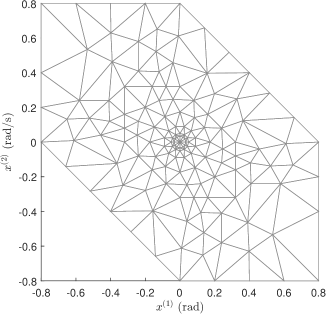
(a) The set $\Omega$ and its triangulation on which the storage function and $\gamma$ were found

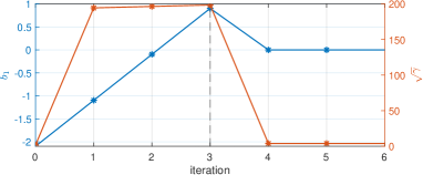
(b) The $b_{1}$ and $\sqrt{\gamma}$ values produced by the iterative algorithm. After three iterations, a positive $b_{1}$ was found. Subsequent steps minimized $\gamma$ while keeping $b_{1}$ positive.

Figure 1: Finding a storage function and the corresponding gain, $\sqrt{\gamma}$

Next, a barrier function and $\hat{u}$ were sought to find a region from which the state would not escape. The boundaries of the sets $\hat{\Omega}$ and $\mathcal{A}_{1}$, where $\mathcal{A}_{1}\subset\hat{\Omega}$, are in dark gray in Fig.2(a). Note that $\hat{\Omega}$ in Fig.2(a) equals $\hat{\Omega}$ but its triangulation is different. Although Theorem 2 does not have any requirement for triangulation of $\hat{\Omega}$ other than that it should cover $\partial\mathcal{A}_{1}$ by the faces of some simplexes, having finer simplexes close to $\partial\hat{\Omega}$ helped to find larger level sets. The simplexes marked by red asterisks in Fig. 2(a) denote the ones on which $D^{+}_{i,j}W$ was not negative on at least one of their vertices. It took only one step to get a positive $b_{2}$ after initializing using Initialization 4. At this point, $\hat{u}$ was $10^{-5}$. Then, by keeping $b_{2}$ positive, $\hat{u}$ was maximized iteratively until it stagnated at $\hat{u}=0.36$ after nine iterations. The $b_{2}$ and $\hat{u}$’s sequences are given in Fig. 2(b). The boundary of $\mathcal{A}$, the largest level set of the obtained barrier function in $\hat{\Omega}$, is depicted in blue in Fig. 2(a).

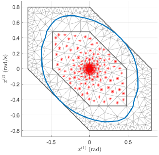
(a) The sets $\hat{\Omega}$ and $\mathcal{A}_{1}$ satisfying $\mathcal{A}_{1}\subset\hat{\Omega}$ and the triangulation on which a barrier function and $\hat{u}$ were found. The boundary of a sub-level set $\mathcal{A}$ satisfying $\mathcal{A}_{1}\subset\mathcal{A}\subset\hat{\Omega}$ is in blue and the boundaries of $\hat{\Omega}$ and $\mathcal{A}_{1}$ are in dark gray. The simplexes with red asterisks are the ones on which $D^{+}W_{i,j}$ was not negative for at least one of their vertices.

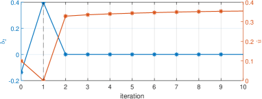
(b) The $b_{2}$ and $\hat{u}$ values produced by the iterative algorithm. After one iteration, a positive $b_{2}$ was found. Subsequent steps maximized $\hat{u}$ while keeping $b_{2}$ positive.

Figure 2: Finding a barrier function, the corresponding $\hat{u}$, and the level-set $\mathcal{A}$

Finally, since $\Omega=\hat{\Omega}$ in this example, Theorem 3 implies that inside $\mathcal{A}$, small-signal finite-gain $\mathcal{L}_{2}$ stability holds with $\sqrt{\gamma}=3.85$ and $\hat{u}=0.36$.

6 Conclusion

This paper presented new criteria employing CPA function approximations and error bounds in order to analyse the small-signal $\mathcal{L}_{2}$-gain of constrained, nonlinear state-space realizations. While finding the tightest possible bound is naturally a nonlinear, non-convex feasibility problem, iterative convex overbounding was used to verify the criteria through a sequence of well-posed SDPs.

7 Acknowledgements

This work is supported by ONR under award #N00014-23-1-2043.

References

- [1] S. Boyd, J. Doyle, Comparison of peak and RMS gains for discrete-time systems, Systems & Control letters 9 (1) (1987) 1–6.
- [2] G. Zames, Feedback and optimal sensitivity: Model meference transformations, multiplicative seminorms, and approximate inverses, IEEE Transactions on Automatic Control 26 (1981) 301–320.
- [3] G. Zames, B. A. Francis, Feedback, minmax sensitivity, and optimal robustness, IEEE Transactions on Automatic Control 28 (1983) 585–601.
- [4] G. Zames, On the input-output stability of time-varying nonlinear feedback systems part one: Conditions derived using concepts of loop gain, conicity, and positivity, IEEE transactions on automatic control 11 (2) (1966) 228–238.
- [5] K. Zhou, J. C. Doyle, Essentials of robust control, Vol. 104, Prentice hall Upper Saddle River, NJ, 1998.
- [6] J. Doyle, K. Glover, P. Khargonekar, B. Francis, State-space solutions to standard and control problems, in: 1988 American Control Conference, IEEE, 1988, pp. 1691–1696.
- [7] S. Boyd, V. Balakrishnan, P. Kabamba, A bisection method for computing the norm of a transfer matrix and related problems, Mathematics of Control, Signals and Systems 2 (3) (1989) 207–219.
- [8] N. Bruinsma, M. Steinbuch, A fast algorithm to compute the -norm of a transfer function matrix, Systems & Control Letters 14 (4) (1990) 287–293.
- [9] L. Guo, L. Xia, Y. Liu, Recursive algorithm for the computation of the -norm of polynomials, IEEE Transactions on Automatic Control 33 (12) (1988) 1154–1157.
- [10] C. Scherer, -control by state-feedback and fast algorithms for the computation of optimal -norms, IEEE Transactions on Automatic Control 35 (10) (1990) 1090–1099.
- [11] W.-W. Lin, C.-S. Wang, Q.-F. Xu, On the computation of the optimal norms for two feedback control problems, Linear Algebra and its Applications 287 (1-3) (1999) 223–255.
- [12] P. Gahinet, P. Apkarian, Numerical computation of the norm revisited, in: Proceedings of the 31st IEEE Conference on Decision and Control, IEEE, 1992, pp. 2257–2258.
- [13] A. Gattami, B. Bamieh, Simple covariance approach to analysis, IEEE Transactions on Automatic Control 61 (3) (2015) 789–794.
- [14] P. Benner, T. Mitchell, Faster and more accurate computation of the norm via optimization, SIAM Journal on Scientific Computing 40 (5) (2018) A3609–A3635. doi:10.1137/17M1137966.
- [15] M. Xia, P. Gahinet, N. Abroug, C. Buhr, E. Laroche, Sector bounds in stability analysis and control design, International Journal of Robust and Nonlinear Control 30 (18) (2020) 7857–7882.
- [16] A. J. Van Der Schaft, -gain analysis of nonlinear systems and nonlinear state feedback control, IEEE Transactions on Automatic Control 37 (6) (1992) 770–784.
- [17] J. A. Ball, J. W. Helton, Viscosity solutions of hamilton-jacobi equations arising arising in nonlinear control, in: control, J. Math. Systems Estim. Control, Citeseer, 1996.
- [18] J. W. helton, M. R. James, Extending Control to Nonlinear Systems: Control of Nonlinear Systems to Achieve Performance Objectives, SIAM, 1999.
- [19] H. Zhang, P. M. Dower, Performance bounds for nonlinear systems with a nonlinear -gain property, International Journal of Control 85 (9) (2012) 1293–1312.
- [20] E. Summers, A. Chakraborty, W. Tan, U. Topcu, P. Seiler, G. Balas, A. Packard, Quantitative local -gain and reachability analysis for nonlinear systems, International Journal of Robust and Nonlinear Control 23 (10) (2013) 1115–1135.
- [21] E. Warner, J. Scruggs, Iterative convex overbounding algorithms for BMI optimization problems, IFAC 50 (1) (2017) 10449–10455.
-
[22]
H. Khalil, Nonlinear
Systems, Pearson Edu, Prentice Hall, 2002.
URL https://books.google.com/books?id=t_d1QgAACAAJ - [23] P. A. Giesl, S. F. Hafstein, Revised CPA method to compute Lyapunov functions for nonlinear systems, J Math Analysis & Apps 410 (1) (2014) 292–306.
- [24] R. Lavaei, L. Bridgeman, Simultaneous controller and Lyapunov function design for constrained nonlinear systems, in: 2022 American Control Conference (ACC), IEEE, 2022, pp. 4909–4914.
- [25] R. Lavaei, L. J. Bridgeman, Systematic, Lyapunov-based, safe and stabilizing controller synthesis for constrained nonlinear systems, IEEE Transactions on Automatic Control (2023) 1–12doi:10.1109/TAC.2023.3302789.
- [26] P. Giesl, S. Hafstein, Construction of Lyapunov functions for nonlinear planar systems by linear programming, J. Math. Anal. Appl. 388 (1) (2012) 463–479.
- [27] A. D. Ames, X. Xu, J. W. Grizzle, P. Tabuada, Control barrier function based quadratic programs for safety critical systems, IEEE Trans Aut Ctrl 62 (8) (2016) 3861–3876.
-
[28]
P. Giesl, S. Hafstein, Computation and
verification of Lyapunov functions, SIAM J on Appl Dyn Sys 14 (4) (2015)
1663–1698.
arXiv:https://doi.org/10.1137/140988802, doi:10.1137/140988802.
URL https://doi.org/10.1137/140988802 - [29] S. Boyd, L. El Ghaoui, E. Feron, V. Balakrishnan, Linear Matrix Inequalities in System and Control Theory, Vol. 15 of Studies in Applied Mathematics, SIAM, Philadelphia, PA, 1994.
- SDP
- semi-definite program
- MPC
- model predictive control
- CLF
- control Lyapunov function
- CBF
- control barrier function
- CPA
- continuous piecewise affine
- QP
- quadratic programming
- DP
- dynamic programming
- ROA
- region of attraction
- PWA
- piecewise affine
- LMI
- linear matrix inequality
- BMI
- bilinear matrix inequality
- EMPC
- explicit model predictive control
- HJ
- Hamilton-Jacobi