Ordering kientics and steady states of XY-model with ferromagnetic and nematic interaction

Abstract

The two-dimensions XY-model, undergoes the Berezinskii Kosterlitz Thouless (BKT) transition through unbinding of defect pairs of opposite signs. When the interaction between spins is purely ferromagnetic, these defects have $\pm 1$ charge, whereas for pure nematic interaction between spins, they have charge $\pm 1/2$. Two-dimensional XY-model in the presence of both ferromagnetic and nematic interactions has been studied both theoretically and experimentally. In this paper, we have studied dynamics of defects in the presence of both ferromagnetic and nematic interactions on a square lattice. Varying the strength of ferromagnetic and nematic interactions, we have observed behavior of both integer and half integer defects and based on that we propose a phase diagram which exhibit three distinct regions in the phase diagram below the critical $T_{BKT}$ : polar phase, nematic phase and coexistence phase and a disordered regions above it. Also, for pure polar and pure nematic case, our results show that the exponent, for algebraic decay of number of defects with time, decays linearly with temperature.

I Introduction

According to Mermin Wagner theorem Mermin (1967); Hohenberg (1967); Mermin and Wagner (1966), in two-dimensions it is impossible for any system to exhibit a long range order by spontaneous breaking of continuous symmetry. $XY$-model comes under this category and hence exhibits Quasi Long Range Order (QLRO) instead of true long range order (LRO) Chaikin and Lubensky (1995); Alba et al. (2009); Goldenfield (2018). So, a conventional phase transition from an ordered state to a disordered state is not possible in a two-dimensional XY model. Brazenskii, Kosterlitz, and Thouless Kosterlitz and Thouless (1973) predicted a special type of phase transition from a disordered state to a QLRO state, which occurs through binding-unbinding of vortices as the system is quenched from high temperature to low temperature below $T_{KT}$. This special type of phase transition is known as Kosterlitz Thouless (KT) transition Kosterlitz and Thouless (1973); Vanderstraeten et al. (2019); Mila (1993); Richter-Laskowska et al. (2018). Generally, a phase transition is characterized by an order parameter that has a nonzero value in the ordered phase and zero in the disordered state. But KT transition can not be explained in a similar fashion; rather, it can be understood as: For XY model in two-dimensions, Long range order is destroyed due to the presence of defects. For $T<T_{KT}$, the formation of isolated defects can cause $+ve$ change in free energy. So, the free energy of the system diverges for $L\to\infty$ Chaikin and Lubensky (1995); Goldenfield (2018); Jensen (2003); Packard (2013). So the system is unstable for the formation of isolated defects and two defects of opposite signs are bound in pairs. But for $T>T_{KT}$, the formation of isolated defect minimizes the free energy. Thus, as the temperature of the system is increased from low to above $T_{KT}$, defect pairs unbind, and the system goes to a disordered state.
The KT transition can be characterized by two-point spin correlation function: $G_{1}(r)=\bigg{<}\cos[\theta(r_{0})-\theta(r_{0}+r)]\bigg{>}_{r_{0}}$ for system with ferromagnetic interaction between the spins Korshunov (1985). For $T<T_{KT}$, correlation function decays algebraically, $r^{-\eta}$ with $\eta=\frac{T}{2\pi J}$ Chaikin and Lubensky (1995); Goldenfield (2018); Jensen (2003); Packard (2013); Yurke et al. (1993), and in the disordered state it decays exponentially. As the temperature is increased, $\eta$ increases and takes value $\frac{1}{4}$ at $T=T_{KT}$.

When the interaction between the spins is apolar Lebwohl and Lasher (1972); Tang and Selinger (2018) then the nature of the defects changes, but the ordered state remains QLRO. In this case, the KT transition can be characterized by the nematic two-point correlation function: $G_{2}(r)=\bigg{<}\cos[2\theta(r_{0})-2\theta(r_{0}+r)]\bigg{>}_{r_{0}}$. Its behavior is similar to that with ferromagnetic interaction between the spins. Where the factor of $2$ with $\theta$, takes care of $\theta\rightarrow\theta+\pi$ symmetry of the apolar system.

XY model in two-dimensions in the presence of both ferromagnetic and apolar interactions is very well studied theoretically Carpenter and Chalker (1989); Benakli and Granato (1997); Qin et al. (2009); Žukovič (2016); Park et al. (2008); Maccari et al. (2020a); Poderoso et al. (2011); Lee and Grinstein (1985) with supported experimental results Qi et al. (2013) of different materials. Since each spin now has both ferromagnetic and apolar interaction probability, the dynamics of the system depend strongly on the strength of the two types of interaction, and this competition between them gives some interesting results. A study of the phase diagram in the interaction strength and temperature plane reveals the existence of three phases: a Ferromagnetic Phase, a Nematic Phase below, and a disordered phase above the transition temperature, respectively. Ferromagnetic $\to$ disordered $\&$ nematic $\to$ disordered transitions are identified as KT transitions, whereas the transition ferromagnetic $\to$ nematic is identified to be a 2-dimensional-Ising type transition and also found in experiments Qi et al. (2013). Although the phase transition is studied for system mixed ferromagnetic/apolar interaction, the details of defect dynamics for the system are not yet explored. In this work, we intend to study the dynamics of defects in two-dimensional-XY model in the presence of both types of interactions.

In our model, spins are distributed on a two-dimensional square lattice, where each spin is assigned a finite probability for interacting either ferromagnetically or nematically with its neighboring spins. By manipulating the interaction strength and temperature as tuning parameters, our primary focus is to analyze the behaviors of defects under diverse conditions. Our observations uncover intriguing defect dynamics. The key outcomes of our study are as follows: (i) In systems characterized by purely polar or purely nematic interactions, the process of defect annihilation is notably slower; (ii) In scenarios where there exists a finite probability for both types of defects, we discover distinct phases emerging based on different combinations of parameters. Particularly, when the probabilities of ferromagnetic and anti-ferromagnetic interactions are comparable, we identify a state where both types of defects coexist within the system.

The forthcoming organization of this paper is structured as follows: Section II provides an elaborate discussion of the particulars of our model. Section III delves into the results, where we first examine the dynamics of defects in a Pure Polar System in Section III.1.2, followed by an analysis of the Pure Nematic System in Section III.1.3. We then extend our analysis to Mixed Systems in Section III.1.4. Next, we illustrate the Phase Diagram in Section III.2. Finally, our study is encapsulated in Section IV, where we offer a comprehensive summary of our findings.

II Model

Our model considers a square lattice with spins arranged at unit lattice spacing. Each spin is represented by an angle $\theta$ ranging from 0 to $2\pi$. We express the spin as a vector $\vec{S}\equiv(\cos\theta,\sin\theta)$, where the magnitude is normalized to unity, i.e., $|\vec{S}|=1$.

Here, the Hamiltonian of the classical XY model incorporates both ferromagnetic and nematic interactions, leading to the following modified form:

$$H=-\Delta\sum_{<ij>}\cos(\theta_{ij})-(1-\Delta)\sum_{<ij>}\cos(2\theta_{ij})$$ (1)

Here, $\theta_{ij}$ denotes the angle between spins $i$ and $j$, defined as $\theta_{ij}=\theta_{i}-\theta_{j}$. The summation is taken over pairs of nearest neighbors, indicated by $<ij>$. The parameters $\Delta$ and $(1-\Delta)$ correspond to the strengths of ferromagnetic and nematic interactions, respectively. The limits $\Delta=1$ and $\Delta=0$ correspond to the pure ferromagnetic (polar) and pure nematic (apolar) cases, respectively. For intermediate values of $\Delta$ within the range $(0,1)$, spins can adopt either type of interaction with probabilities determined by $\Delta$ and $(1-\Delta)$. We label the system as “Pure Polar” when $\Delta=1$, “Pure Nematic” when $\Delta=0$, and “Mixed” for $0<\Delta<1$.

To simulate the system, we employ the Metropolis-Monte Carlo method on the square lattice of size $L\times L$ with periodic boundary conditions in both directions. A simulation step is completed when each spin has been attempted once. Distances are measured in terms of the lattice spacing, and we set the Boltzmann constant $k_{B}$ to unity for consistency. The presented results are based on a system size of $(L=256)$ unless stated otherwise. To ensure statistical accuracy, data are averaged over a minimum of $100$ independent realizations. Each realization involves simulating the system for $3\times 10^{4}$ steps for a $L=256$ system, or $7\times 10^{4}$ steps for a $L=512$ system.

III Results

III.1 Defect Dynamics

We characterized the properties of the system in terms of topological defects. First, we briefly describe the origin and importance of defects in the system with continuous symmetry. Topological defects represent distinct distortions in the state of broken symmetry within a system. In its pursuit of equilibrium, the system seeks to minimize its free energy, hence favoring the ordered alignment of spins with long-range parallel or anti parallel interactions in a ferromagnetic or nematic setting respectively. However, the presence of defects introduces energy penalties. Remarkably, these defects possess topological stability and can only be eliminated through abrupt local changes in spin orientation. Consequently, achieving a defect-free configuration incurs a substantially higher energy cost. Thus, in two dimensions, the system exhibits a preference for configurations that include defects.
Topological defects feature a core where order is completely disrupted, while $\theta(x)$ exhibits slow variation in its distant surroundings. These defects are classified based on the winding number, denoted as $k$, which quantifies the change in $\theta(x)$ along a closed loop encircling the defect. The winding number can be positive or negative, as well as an integer or half-integer. Defects in a system are intimately linked to the nature of its broken symmetry state, which is determined by the specific particle interactions at play. As a result, defects can be seen as unique fingerprints of the system, providing valuable insights into the characteristics of the broken symmetry state.
Upon a sudden temperature quench from above $T>T_{KT}$ to $T<T_{KT}$, the disordered state of the system becomes unstable, triggering the onset of ordering. In this process, defects of opposite signs interact, resulting in their annihilation and the eventual emergence of a homogeneous configuration. As time progresses, the number of defects in the system decreases, ultimately leading to a steady state where only a few defects remain. In two dimensions, the ordering is quasi long-ranged, allowing finite size systems to achieve a defect-free steady state. However, in an infinite size system, this process takes an infinite amount of time, rendering it practically impossible to obtain a defect-free state.
Here, at each time step, we count the number of defects present in the system. Below we show how the defect count in the system varies depending on parameters $T$ and the nature of interaction $\Delta$.

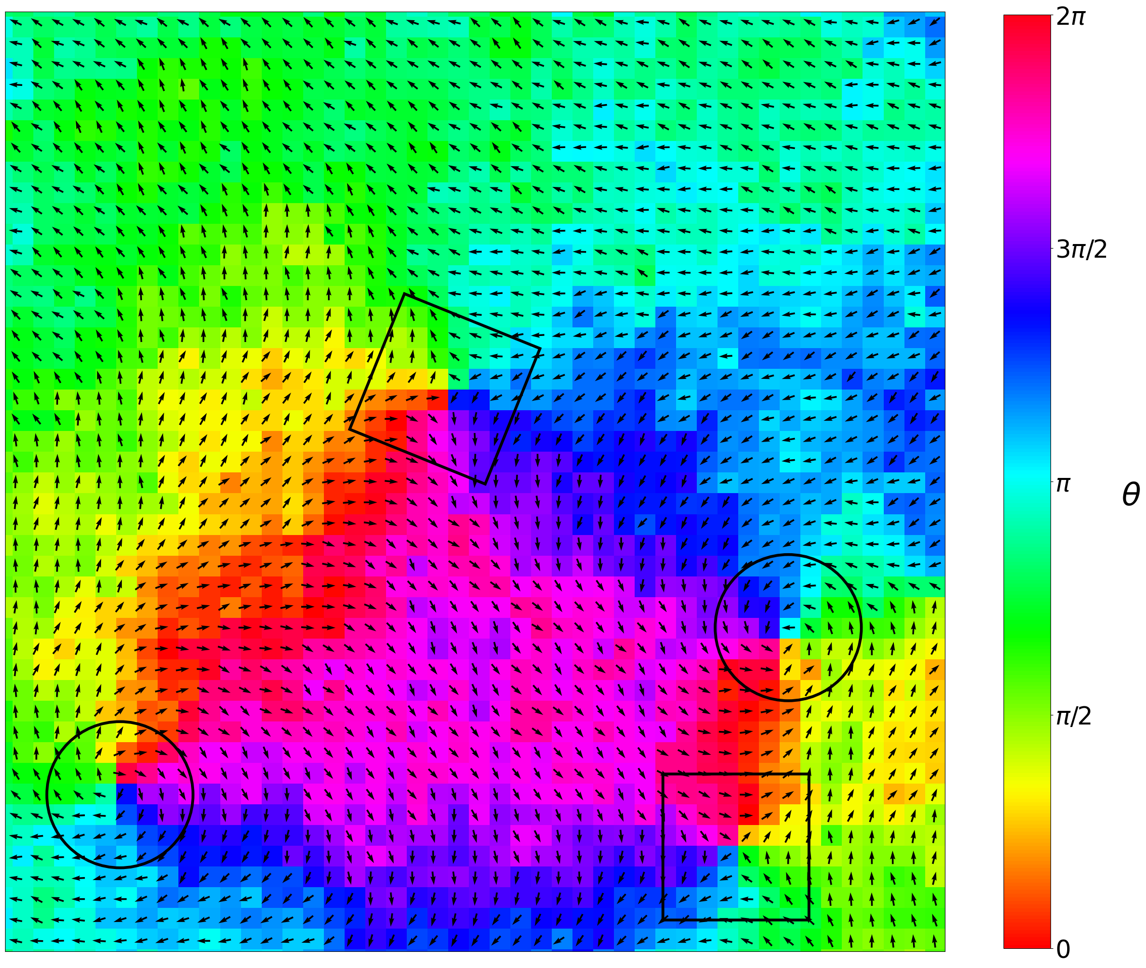
(a)

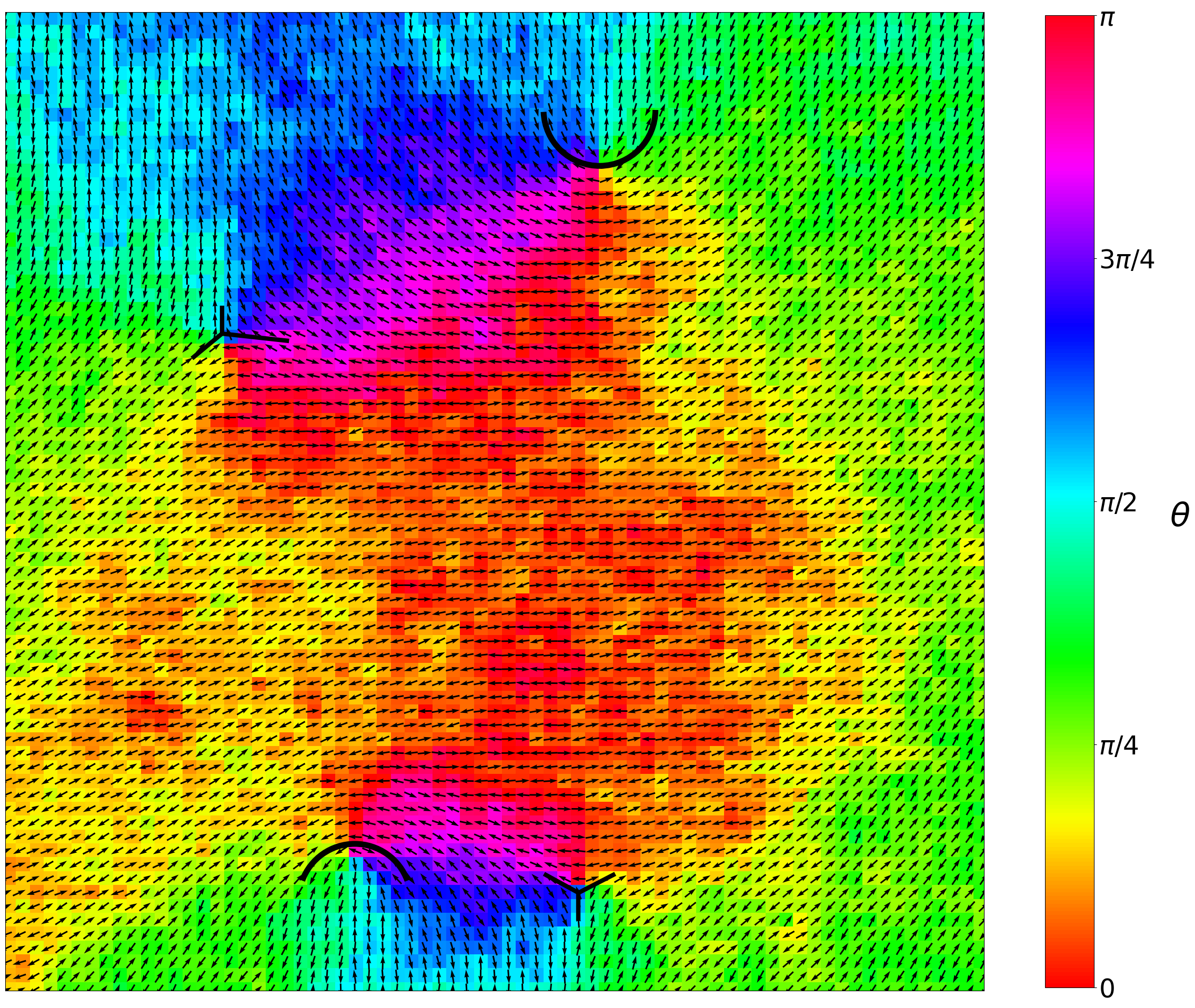
(b)

Figure 1: The figure illustrates defect configurations in the system with pure ferromagnetic interaction, subplot (a), and pure nematic interaction, subplot (b). Background color, in subplots (a) and (b), represents the orientation field, $\theta$, according to the corresponding colorbar and the black quivers represent the spins at each lattice point. (a) shows $\pm 1$ defects with black circle and square, respectively; (b) shows $\pm\frac{1}{2}$ defect configurations marked with black dashed arcs, and ‘Y’-shaped structures, respectively. A part of the system of size $L=128$ is shown for better resolution.

III.1.1 Defect Detection

The defect in the system is obtained by the following method. We first evaluate the rotation of the orientation field around a point $(i,j)$, and evaluate the integral

$$I=\oint_{\Gamma}\vec{\nabla}\theta.d\vec{r}=\oint_{\Gamma}d\theta$$

where, $\Gamma$ is a closed contour around the point $(i,j)$.
This gives,

$$\begin{split}I=\oint_{\Gamma}\vec{\nabla}\theta.d\vec{r}&=2k\pi,\hskip 2.84526ptif\hskip 2.84526pt\Gamma\hskip 2.84526ptencloses\hskip 2.84526pta\hskip 2.84526ptdefectcore\\ &=0,\hskip 2.84526ptotherwise\end{split}$$

Where, $k$ is called the winding number and characterize the type of defect. The winding number at lattice point $(i,j)$ is calculated as,

$$k=\frac{I}{2\pi}$$

Next, we proceed to characterize the properties of the system individually for the cases of pure polar, pure apolar, and mixed scenarios.

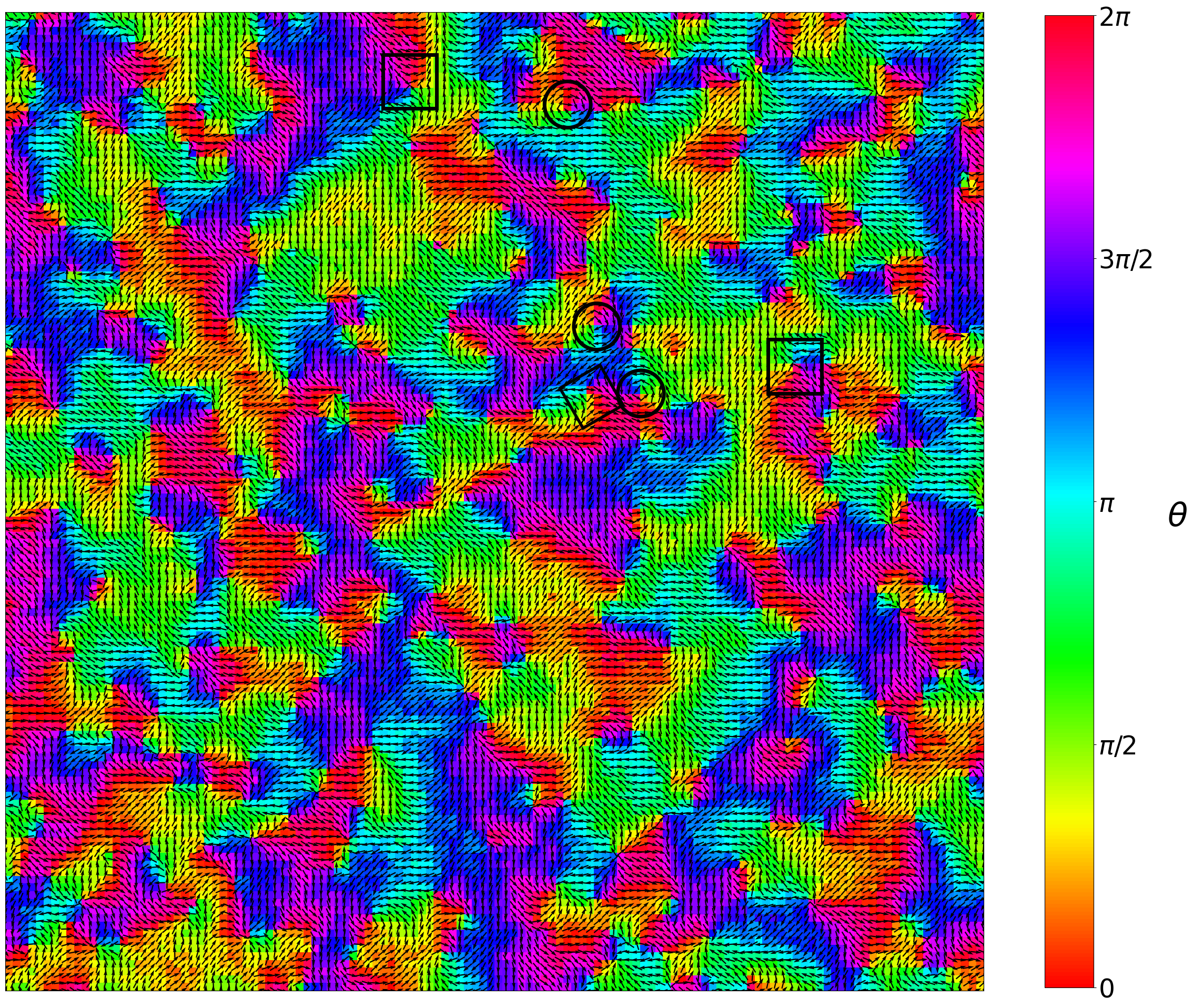
(a)

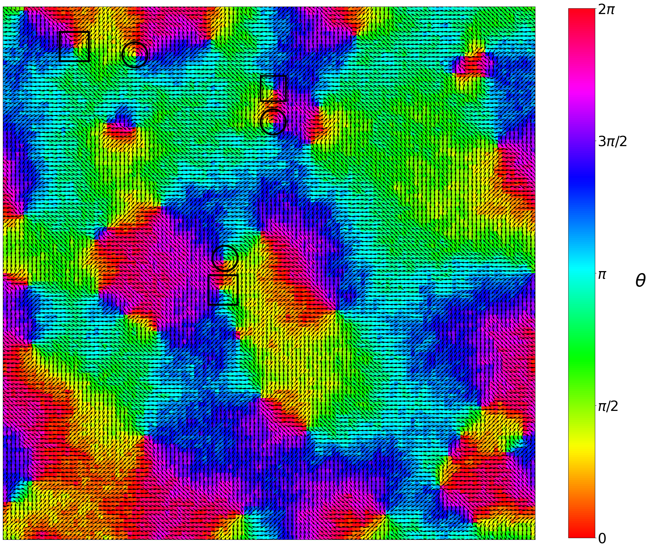
(b)

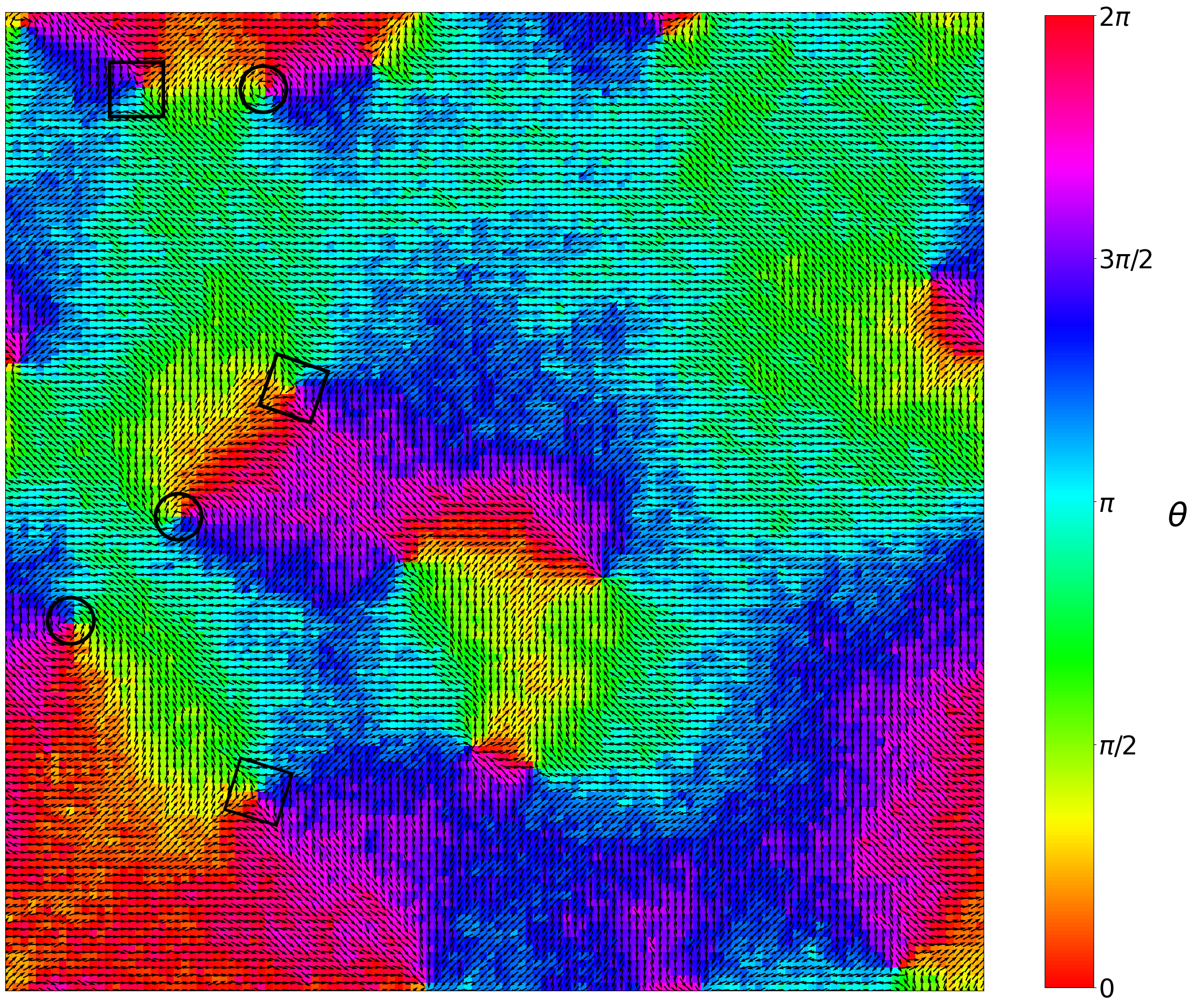
(c)

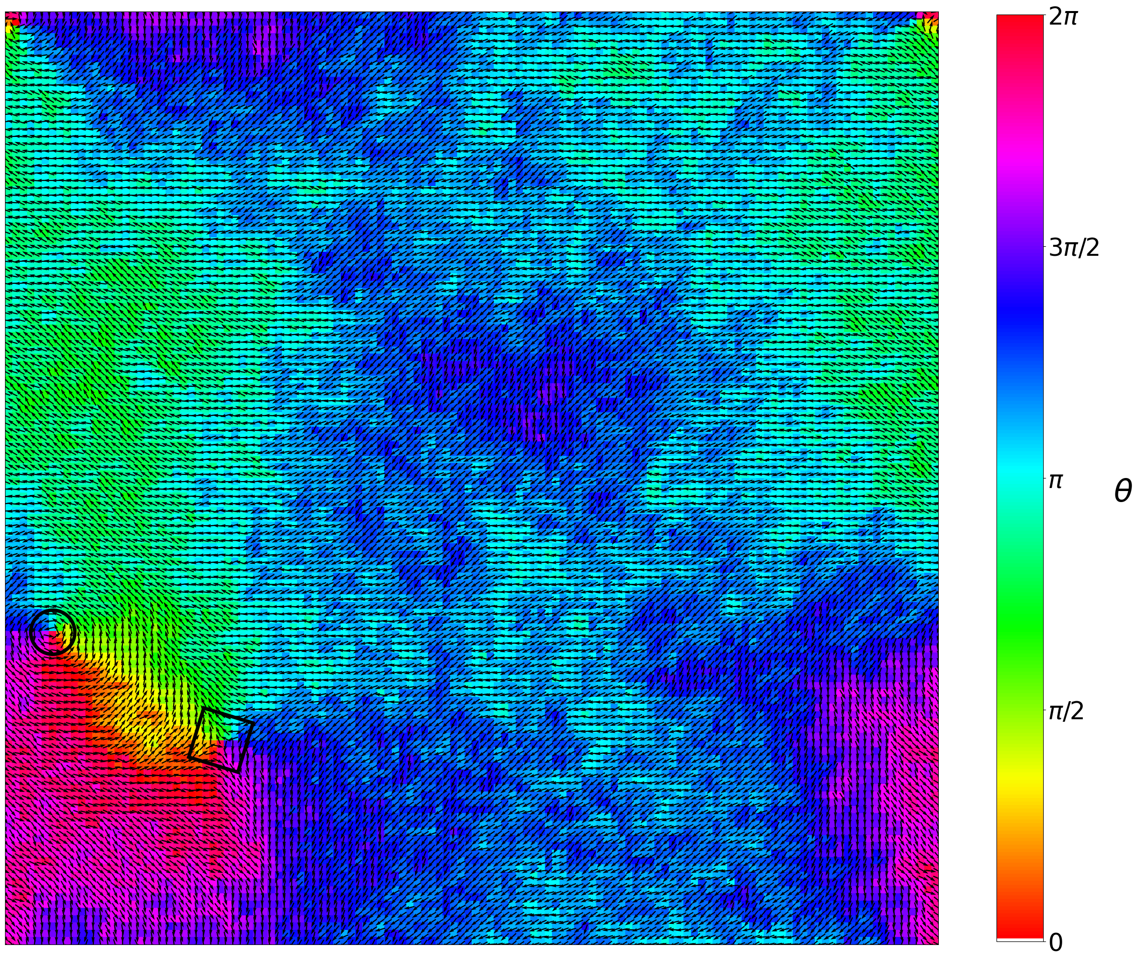
(d)

Figure 2: (color online) The figure provides a visual representation of the evolving Pure Polar System, depicted through a sequence of snapshots. Subplots (a)-(d) exhibit snapshots of the system at distinct time instances: 200, 1000, 2000, and 6000, respectively. In each subplot, the background color denotes the orientation field of spins, indicated by the accompanying color bar, while the black quivers illustrate the spins themselves. Notably, subplots (a)-(d) highlight certain $+1$ and $-1$ defects, marked by black circles and squares, respectively; System Size L = $128$ and $T=0.3$.

III.1.2 Pure Polar System

In a system governed solely by ferromagnetic interactions, stable defect configurations manifest as vortices ($k=+1$) and anti-vortices ($k=-1$), as shown in fig.1(a). These defects exhibit diffusive behaviorMuzny and Clark (1992); Pleiner (1988) and can move through the system. Upon collision, oppositely charged defects annihilate, leading to the emergence of a locally homogeneous, uniformly oriented state. The fig.2 captures the temporal evolution of the system, while the decay in the number of defects over time is illustrated through the $N_{p}(t)$ $vs.$ $t$ plot at various temperatures, as depicted in fig.3(c). In this representation, $N_{p}(t)$ quantifies the proportion of defects that persist in the system at time $t$, relative to their abundance at the start of the observation, mathematically expressed as $N_{p}(t)=\frac{1}{2}\left[{\sum}_{k=+1}^{-1}\frac{n_{k}(t)}{n_{k}(1)}\right]$, where $n_{\pm 1}(t)$ signifies the count of $k=\pm 1$ defects at time $t$. Across all temperatures where $T<T_{KT}$, the $N_{p}(t)$ $vs.$ $t$ plot exhibits a power-law decay characterized by $N\sim t^{-\alpha_{p}}$. Previous studies of the same have established that in a system of spins interacting solely through ferromagnetic interactions, the exponent $\alpha_{p}$ is approximately 1 Jelić and Cugliandolo (2011); Koo et al. (2006); Yurke et al. (1993). However, in our study, we have observed that $\alpha_{p}(T)$ exhibits temperature dependence. Specifically, when the temperature is significantly lower than the critical temperature $T_{KT}$, $\alpha_{p}(T)$ maintains a value close to 1, which concurs with previous research findings. However, as the temperature is increased, there is a noticeable reduction in the value of $\alpha_{p}(T)$. This particular behavior of $\alpha_{p}(T)$ can be explained as follows:
The motion of defects in the system is governed by the interplay between two fundamental factors: the cooperative interaction between spins, which promotes alignment, and the thermal energy of the spins, which introduces randomness. At extremely low temperatures ($T\ll T_{KT}$), the thermal energy is negligible compared to the dominant spin interaction, resulting in the prevalence of well-defined spin waves Maccari et al. (2020b). This regime is characterized by a nearly constant value of $\alpha_{p}$ close to 1, and the cooperative behavior of spins dominates. However, as the temperature increases, the thermal energy starts to play a more significant role, leading to an increased frequency of random spin flips. Moreover, elevation in temperature induces transverse fluctuations in the well-ordered spin arrangement, leading to a reduction in spin wave stiffness. Consequently, the system becomes more susceptible to a broader spectrum of spin orientation fluctuations in terms of frequency. This alteration in spin wave stiffness results in the localization of defects, while the combined effect of reduced defect dynamics and an increased defect count within the system contributes to a slowing down of the decay rate of the defect population. As a consequence, the $N_{p}(t)$ $vs.$ $t$ curve depicted in fig.3(a) exhibits a flattened profile, and the decay exponent in fig.3(c) experiences a decline. These observations point to a transition from a regime where spin waves dominate to one where thermally induced dynamics take over as the temperature increases.

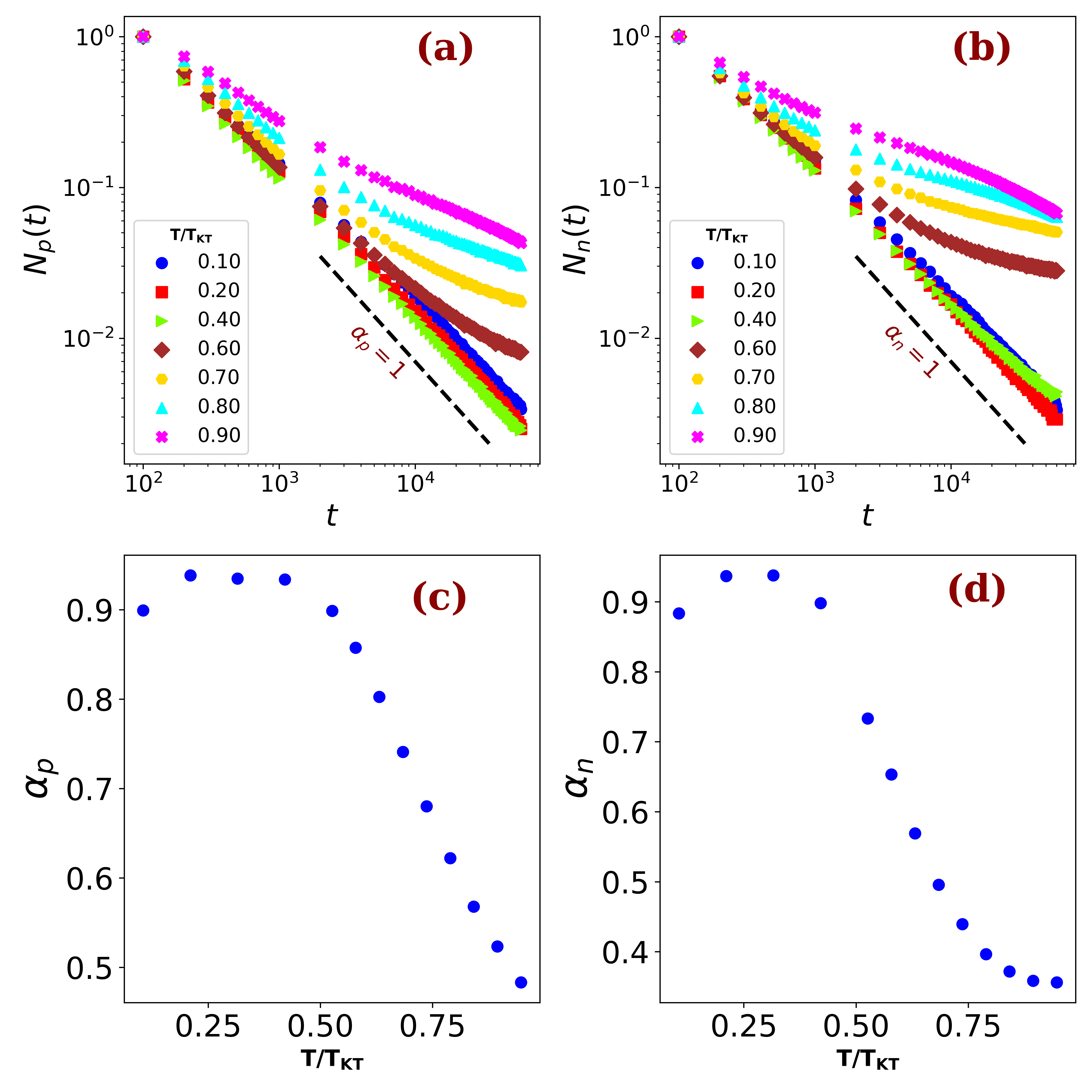
Figure 3: (color online) The figure illustrates the temporal evolution of the system for both the Pure Polar and Pure Nematic cases. In the left panel, subplots (a) and (c) correspond to the Pure Polar scenario, while in the right panel, subplots (b) and (d) depict the Pure Nematic scenario. Subplots (a) and (b) showcase the decay of defect count in the respective systems on log-log scale at different temperatures. In both subplots, the black dashed line represents a power-law decay with an exponent of 1. Subplots (c) and (d) display the variation of the exponent with temperature for the corresponding systems. System Size $L=$ 256.

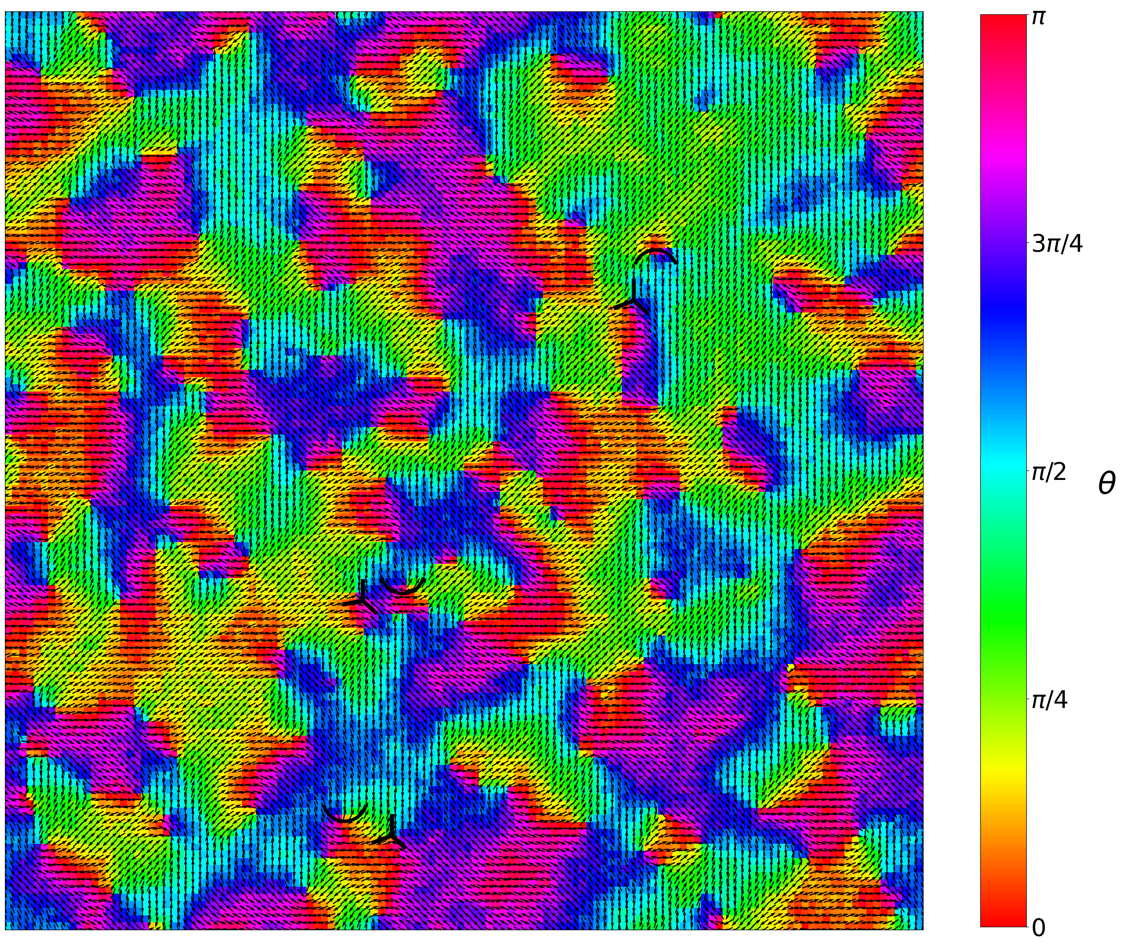
(a)

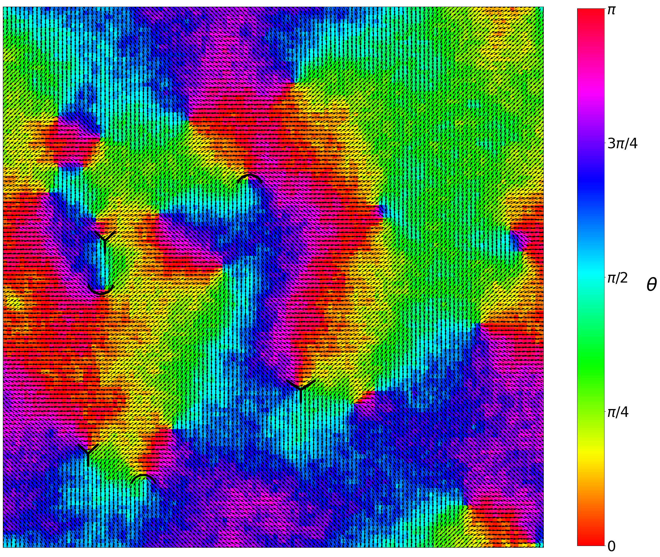
(b)

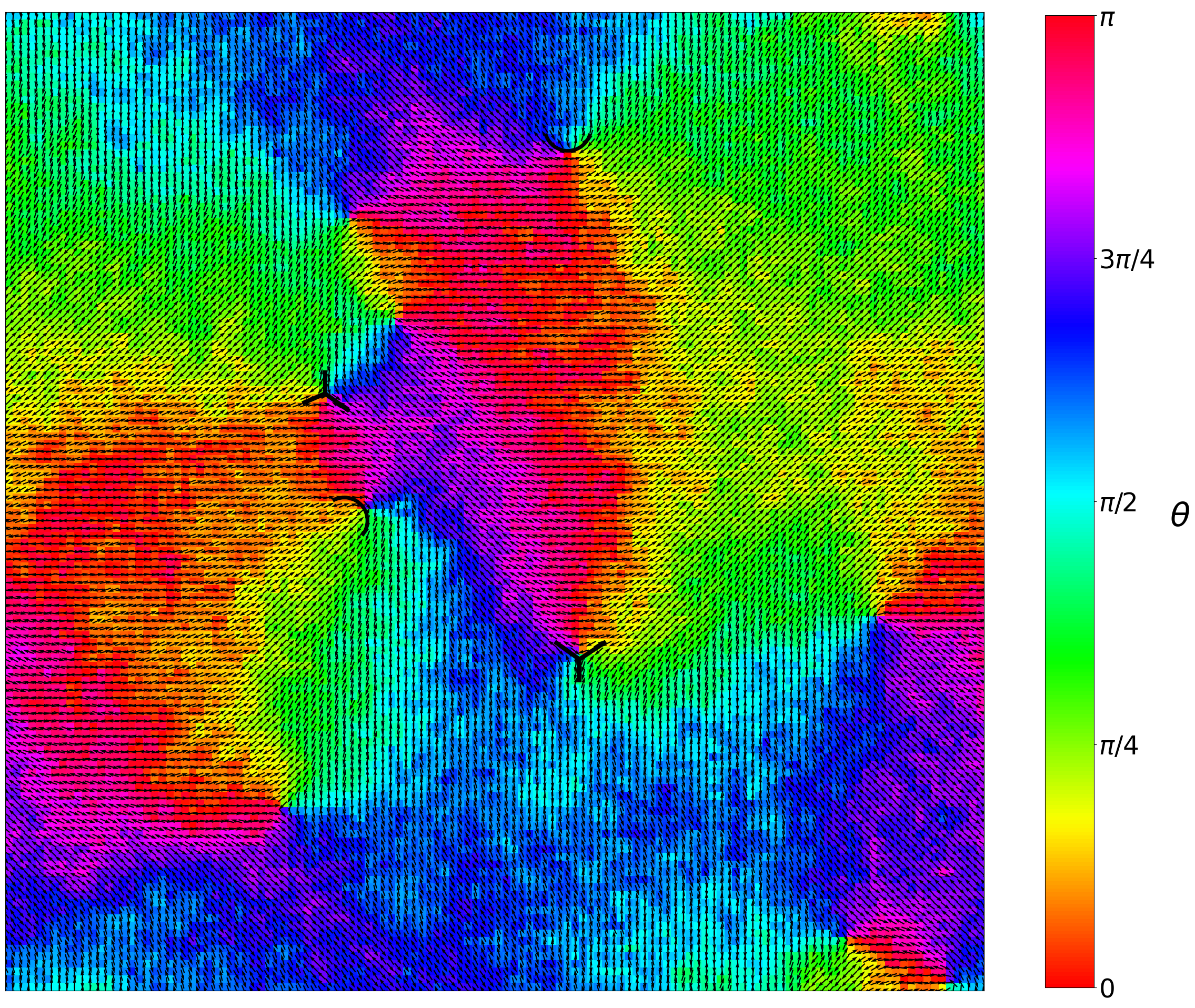
(c)

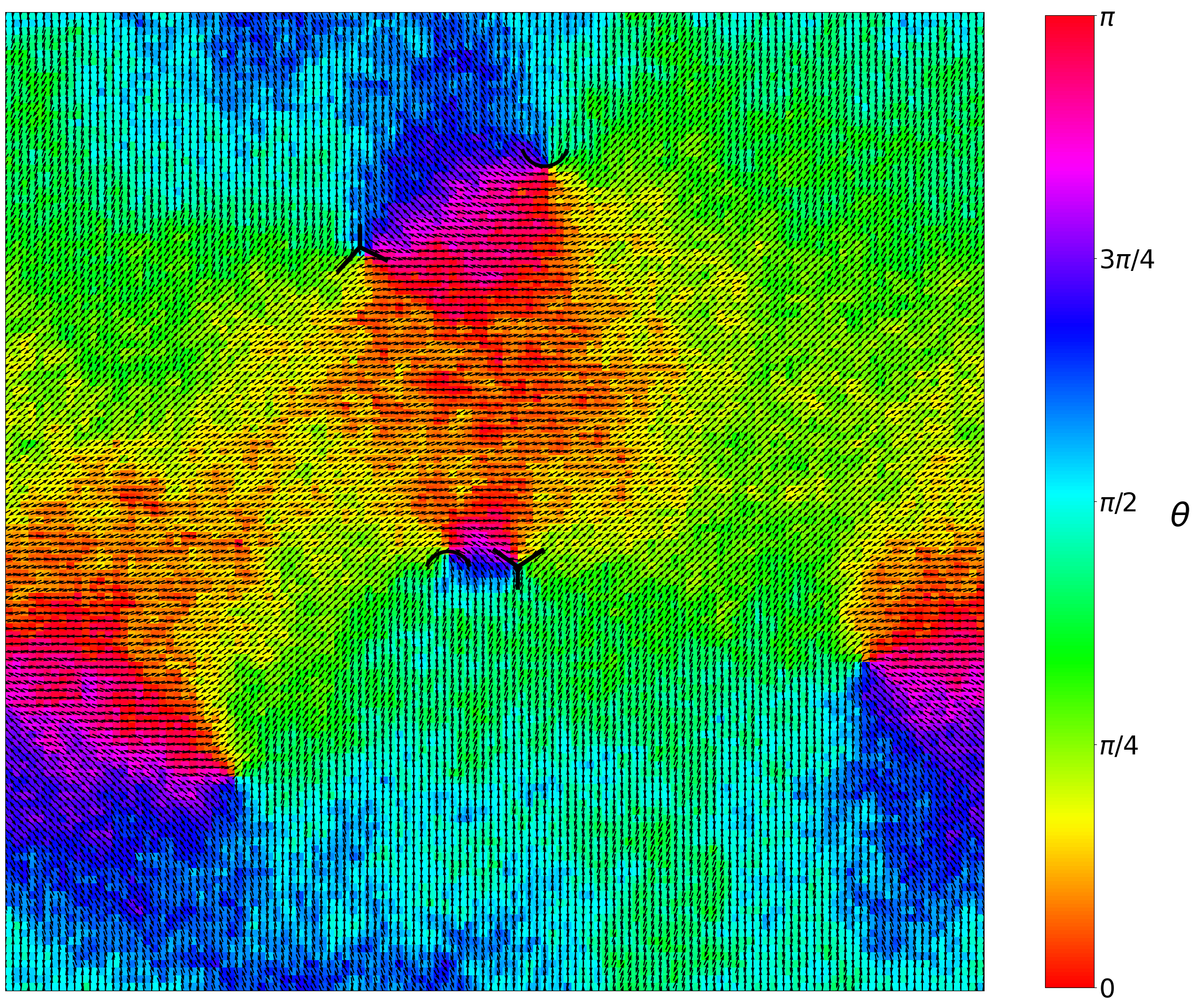
(d)

Figure 4: The presented figure captures the dynamic evolution of a Pure Nematic System, depicted sequentially through a set of snapshots. Subplots (a)-(d) present snapshots of the system taken at distinct time instances: 100, 1000, 2000, and 6000, respectively. In each subplot, the backdrop color represents the orientation field of spins, while the spins themselves are illustrated by the black quivers. Notably, subplots (a)-(d) prominently showcase distinct $+\frac{1}{2}$ and $-\frac{1}{2}$ defects, which are marked by black arcs and ‘Y’-shaped structures, respectively. The remaining parameters are consistent with fig.2.

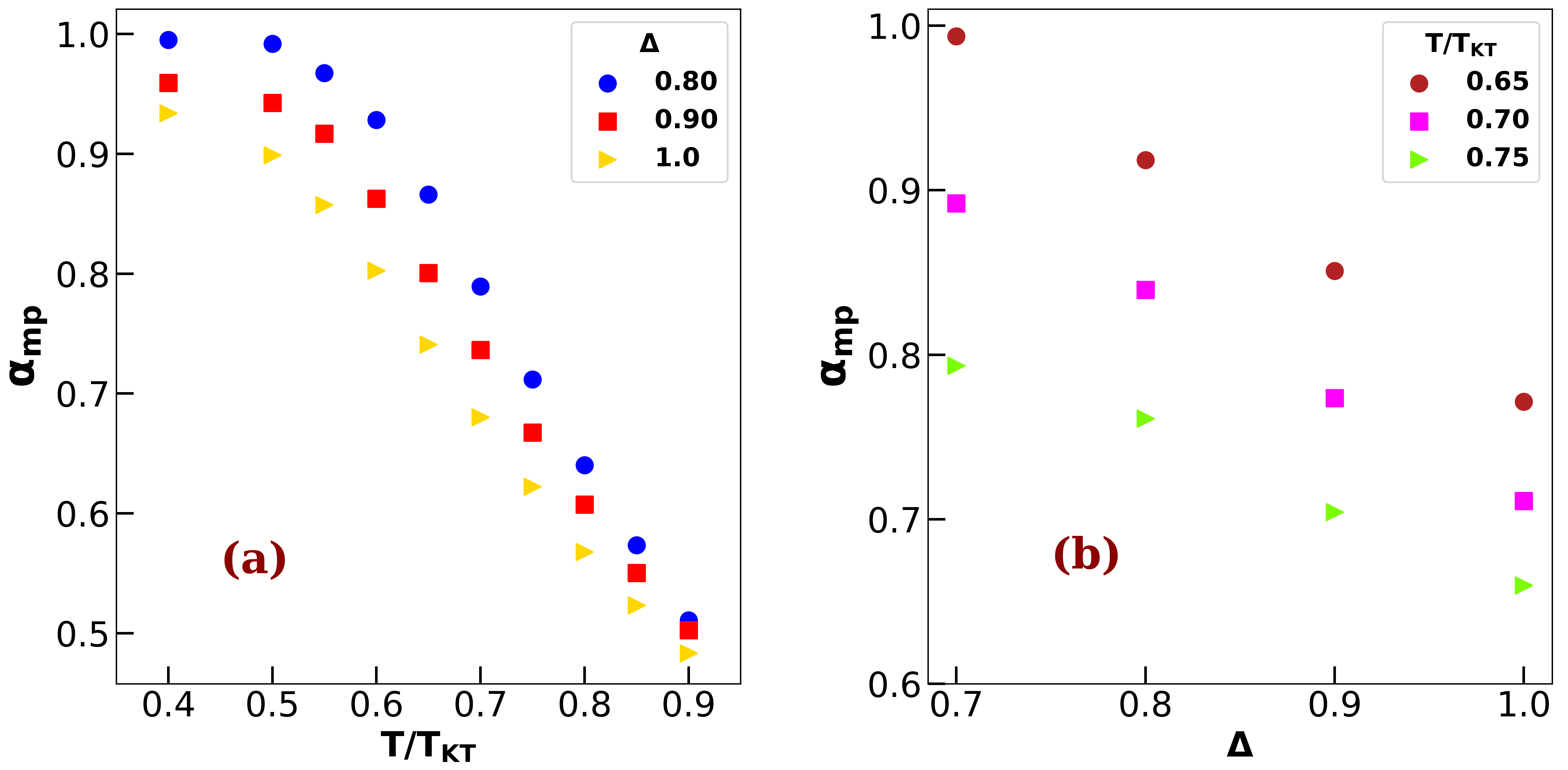
Figure 5: (color online) The figure showcases the variation of the exponent $\alpha_{mp}$ within the Polar Region. Panel (a) displays the exponent’s behavior with temperature for various $\Delta$ values, while panel (b) depicts its variation with $\Delta$ across different temperatures. The remaining parameters remain consistent with those presented in fig.3.

III.1.3 Pure Nematic System

In a system governed by apolar interactions between particles, stable defect configurations correspond to fractional values of $k=\pm\frac{1}{2}$ De Gennes and Prost (1993); Chandrasekhar (1992); Priestly (2012), known as disclination. The spin configurations surrounding the core of these $\pm\frac{1}{2}$ defects are depicted in fig.1(b). Similar to the pure polar system discussed earlier (Section III.1.1), the number of defects in this system also exhibits a time-dependent decay, as observed in the evolution shown in fig.4. The decay follows a power law behavior characterized by $N\sim t^{-\alpha_{n}}$, where $\alpha_{n}$ represents the exponent governing the decay. Previous studies have reported an exponent value of 1 for this decay Hickl (2021); Chuang et al. (1991); Harth and Stannarius (2020). However, our study reveals that similar to the pure polar system, the exponent $\alpha_{n}(T)$ varies with temperature. In the low-temperature regime dominated by spin waves, the exponent remains close to 1, consistent with previous findings. As the temperature rises, the manifestation of a reduced rate of defect annihilation becomes evident through the flattening of the $N_{n}(t)$ $vs.$ $t$ curve, depicted in fig.4(b). Here, $N_{n}(t)$ is defined as, $N_{n}(t)=\frac{1}{2}\left[{\sum}_{k=+\frac{1}{2}}^{-\frac{1}{2}}\frac{n_{k}(t)}{n_{k}(1)}\right]$, where $n_{\pm\frac{1}{2}}(t)$ signifies the count of $k=\pm\frac{1}{2}$ defects at time $t$. Consequently, the exponent of the power law decay, $\alpha_{n}$ decreases as shown in fig.4(d). This behavior can be explained via same argument as given for the polar case: increase in temperature causes decay of reduction of spin wave and localization of defects, finally resulting in slower rate of defect annihilation.

To summarize the previous two sections (Sections III.1.1 and III.1.2), the consideration of systems with different types of interactions allows us to observe distinct characteristics and temperature-dependent behaviors of defect dynamics. In the pure polar system, vortices and anti-vortices play a prominent role, exhibiting diffusive motionMuzny and Clark (1992); Pleiner (1988) and annihilation upon collision. The decay of defects follows a power law with an exponent $\alpha_{p}$ that varies with temperature, indicating the transition from spin-wave-dominated behavior at low temperatures to thermally-driven dynamics at higher temperatures. On the other hand, the pure nematic system showcases disclinations as stable defect configurations. These fractional defects also exhibit a power law decay, with an exponent $\alpha_{n}$, which also varies with temperature. The temperature-dependent behavior reveals the interplay between spin waves and thermal energy in the dynamics of defects.
Next, we show what happens when both type interactions are simultaneously present in the system.

III.1.4 Mixed System

In the mixed system, spins possess the flexibility to choose between ferromagnetic and nematic interactions with their neighbors, each with magnitude $\Delta$ and $1-\Delta$. This characteristic gives rise to distinct behavior in the intermediate range of $\Delta$ values, bridging the gap between the pure polar and pure nematic phases observed in the limiting cases. Our focus in this section is to explore the system’s behavior in the transitional region near the pure polar and nematic limits. To accomplish this, we carefully selected $\Delta$ values that induce subtle deviations from the pure polar and pure apolar systems, enabling us to investigate the intriguing characteristics that emerge in this regime.

Near the polar boundary, we specifically examined three values of $\Delta$ = ($0.8$, $0.9$, and $1.0$). Within this range, we observed the prevalence of $\pm 1$ defects in the system. The decay of the defect population over time exhibited a power law behavior, represented by the relationship $N(t)\sim t^{-\alpha_{mp}(\Delta)}$, where $\alpha_{mp}(\Delta)$ denotes the exponent governing the decay rate. In the low-temperature regime, $\alpha_{mp}(\Delta)$ closely approached $1$, consistent with the behavior observed in the pure polar and pure nematic cases. As the temperature increased, the exponent progressively decreased, as illustrated in fig.5(a). Furthermore, when the temperature remained constant while altering the value of $\Delta$, the parameter $\alpha_{mp}$ exhibited a distinct upward trend, clearly depicted in fig.5(b).

The increasing trend of $\alpha_{mp}$ with increase in $\Delta$ can be explained as follows: Decreasing the parameter $\Delta$ has the effect of reducing the polar nature of individual spins, leading to an increase in the probability of nematic interactions. Previous research has shown that creating a pair of integer defects incurs a significantly higher energy cost compared to a pair of half-integer defects. Consequently, the system tends to preferentially create some half-integer defects at the expense of integer defects. This results in a reduced number of integer defects and a faster rate of annihilation for them, leading to an increase in the parameter $\alpha_{mp}$ at higher temperatures as depicted in fig.5(a). However, at lower temperatures, the system contains only a few defect pairs, and the polar alignment tendency far outweighs the nematic alignment tendency, altering the value of $\Delta$ has minimal impact on the number of defect pairs. As a Consequence, the $\alpha_{mp}$ remains nearly constant and close to 1 for all values of $\Delta$, primarily due to the dominant influence of spin waves.

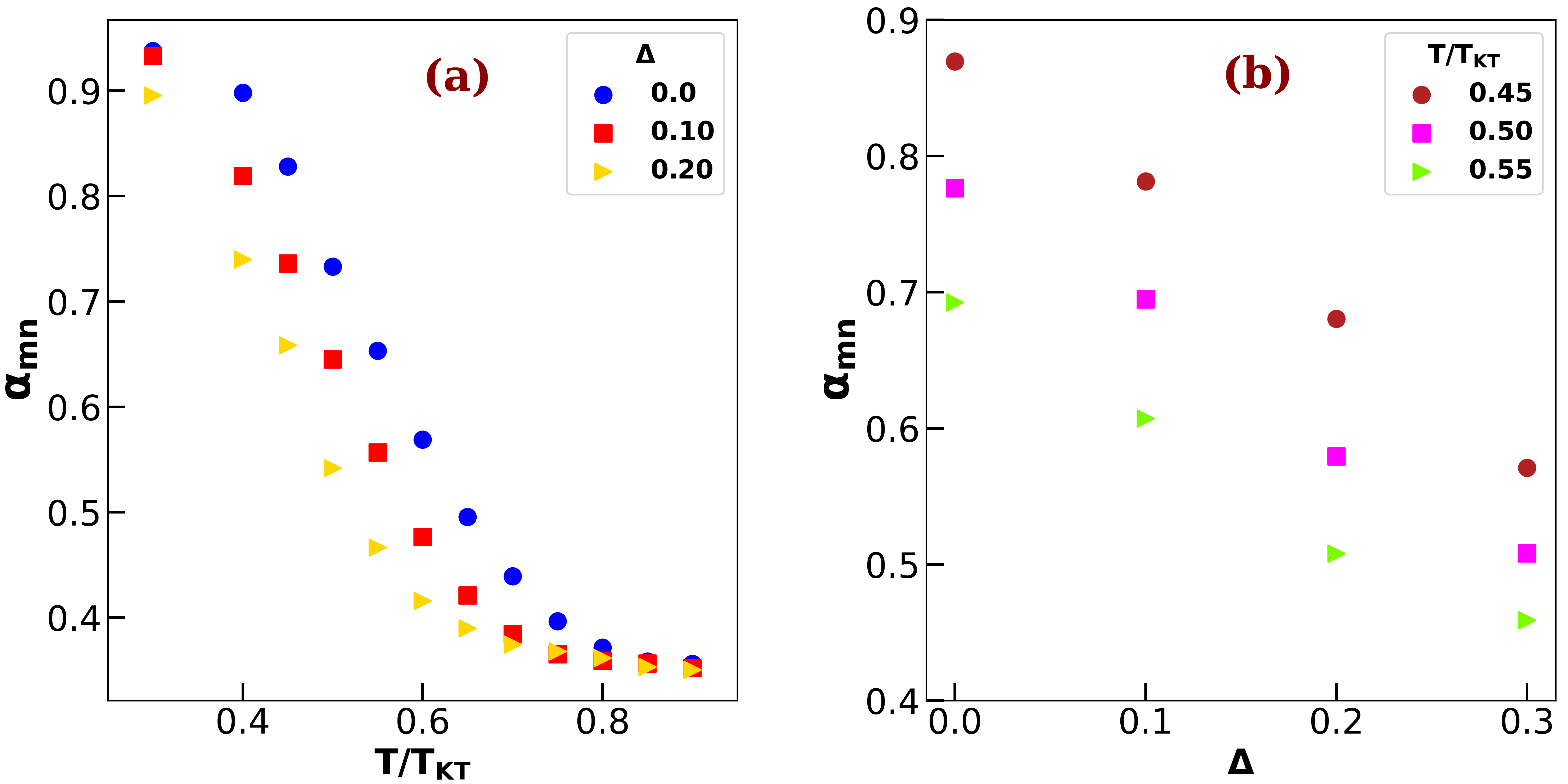
Figure 6: (color online) The depicted figure illustrates the change in the exponent $\alpha_{mn}$ within the Nematic Region. Panel (a) demonstrates the exponent’s temperature dependence for different $\Delta$ values, while panel (b) illustrates its variation with $\Delta$ for different temperatures. Rest of the parameters remain the same as depicted in fig.3.

.

Moving to the vicinity of the nematic boundary, we examined three distinct $\Delta$ values ($0.2$, $0.1$, and $0$). In this regime, the system primarily exhibits $\pm\frac{1}{2}$ defects. The number of defects follows a power law decay: $N\sim t^{-\alpha_{mn}}$, where the exponent $\alpha_{mn}$ remains close to 1 at low temperatures. As the temperature increases, $\alpha_{mn}$ decreases, as illustrated in fig.6(a), consistent with the behavior observed in the pure nematic case. However, in this regime, when $\Delta$ increases from 0 (corresponding to an increased likelihood of polar interactions) at a fixed temperature, $\alpha_{mn}$ also decreases, as shown in fig6(b). The observed behavior can be attributed to the dominance of nematic alignment tendency among neighboring spins at a finite but lower $\Delta$ values. Moreover, the lower energy required to create a half-integer defect leads to the formation of large number of $\pm\frac{1}{2}$ defects at the same temperature. As a result, the annihilation of defects with opposite signs occurs more rapidly, leading to an increased value of $\alpha_{mn}$, as illustrated in fig.6(b).

Overall, these findings demonstrate the intricate interplay between spin interactions, temperature, and defect dynamics in the mixed system, unveiling fascinating behavior in the intermediate region near the pure polar and pure nematic limit.

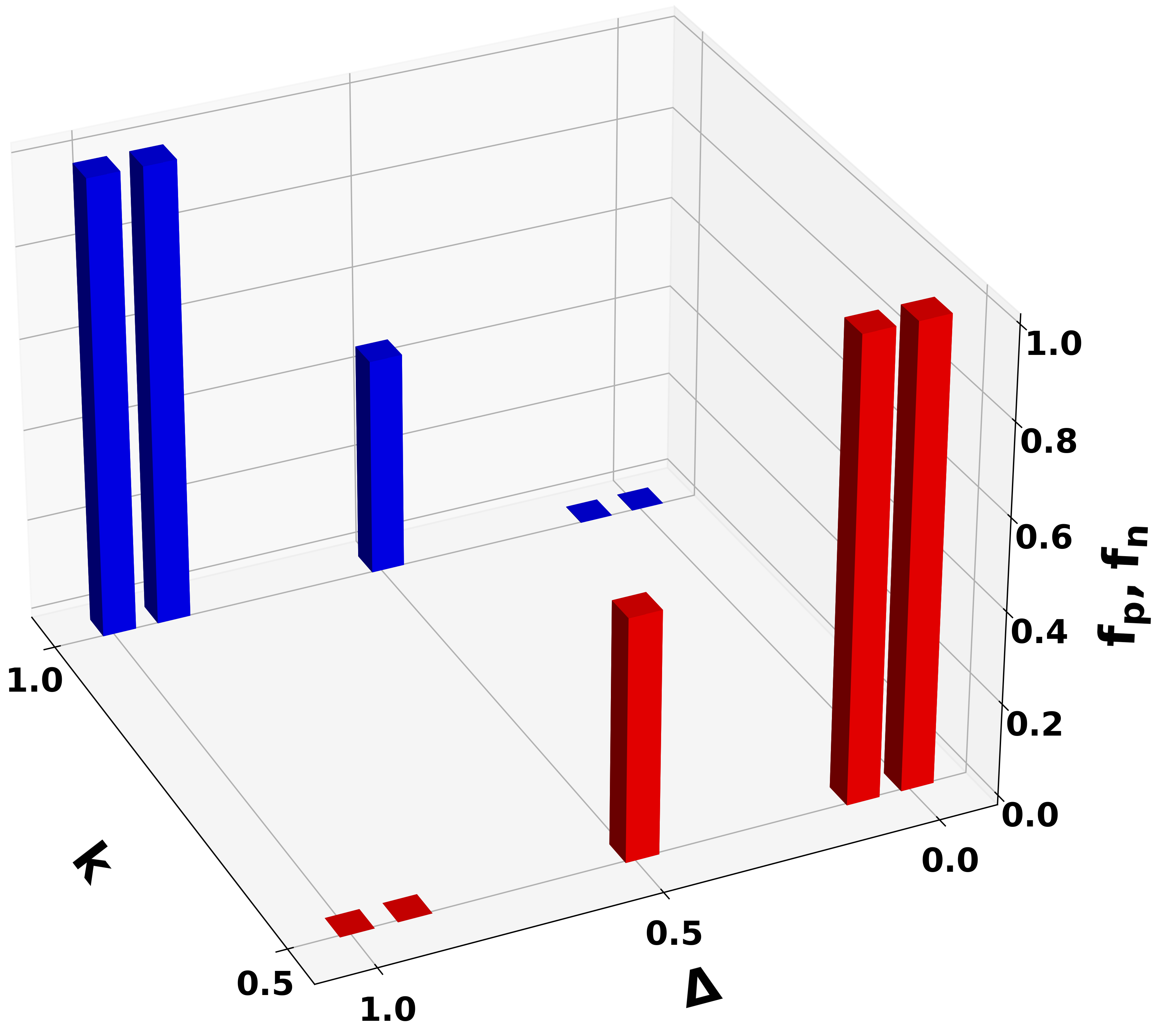
(a)

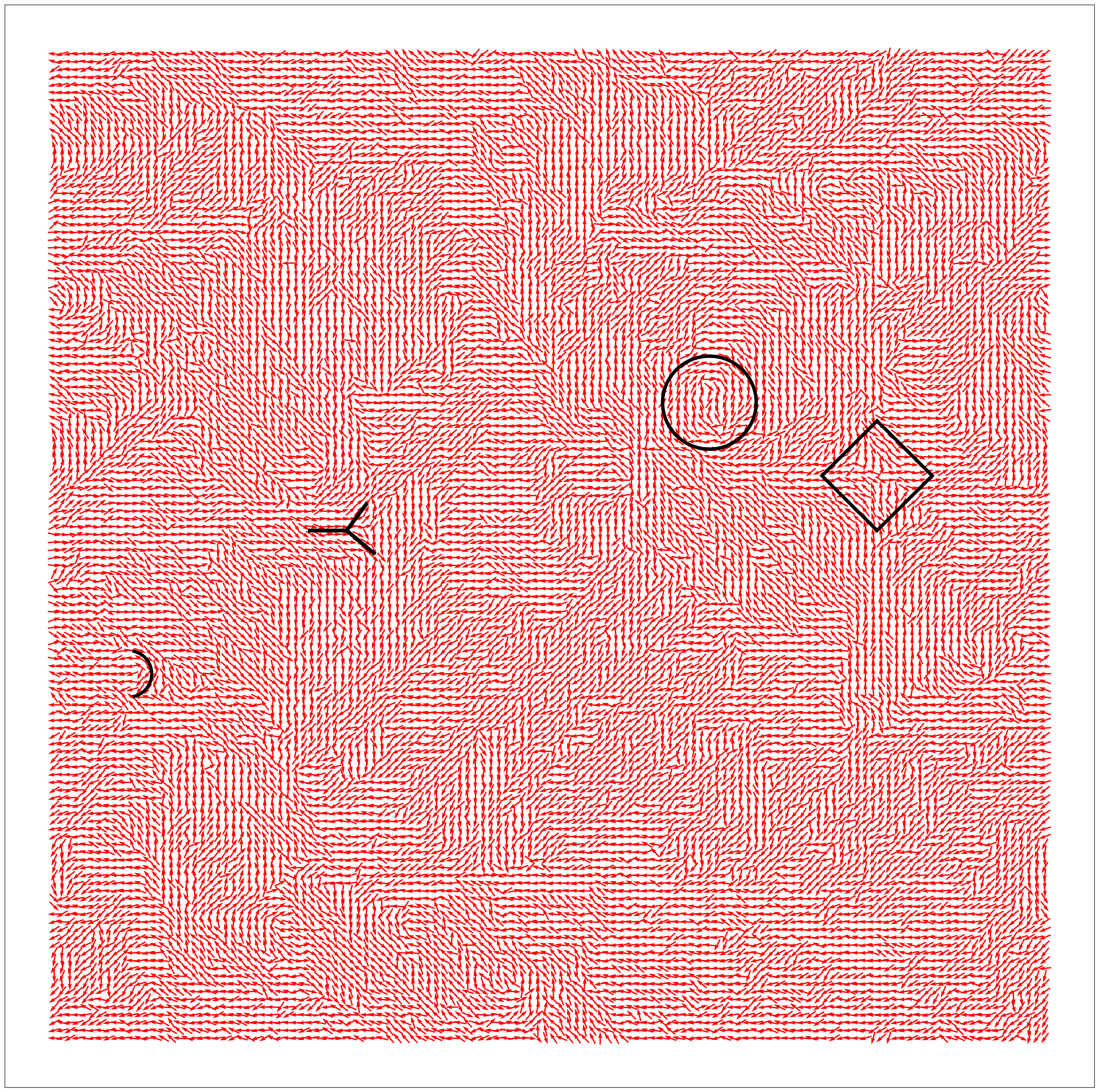
(b)

Figure 7: (color online)(a) The figure depicts the fractions, $f_{p}$ and $f_{n}$, of $\pm 1$ and $\pm\frac{1}{2}$ defects within distinct phases at a temperature of $\frac{T}{T_{KT}}T=0.60$, with the color ’blue’ representing $f_{p}$ and ’red’ indicating $f_{n}$. All other parameters remain consistent with those presented in fig.3; (b) The figure portrays the configuration of the system in a coexistence state at $T=0.6$ and $\Delta=0.50$. In this visualization, spins are depicted as red quivers. a pair of $\pm 1$ defects is denoted by a black circle and square, while a pair of $\pm\frac{1}{2}$ defects is indicated by a black arc and a ’Y’-shaped structure.

III.2 Phase Diagram

In the previous section, we investigated the behavior of defects in pure systems ($\Delta=0$ and $\Delta=1$) as well as in the mixed system near the boundaries of pure polar and pure nematic interactions. By analyzing the exponent of the power law decay of the defect population, we discerned the impact of temperature in the pure systems and the effect of varying $\Delta$ in the mixed system.

Continuing with our analysis, we delve into the characterization of various phases within the system by investigating the behavior of defects across the entire parameter space of $\Delta$ and $T$. Our observations indicate the existence of three distinct phases below $T_{KT}$ : Polar Phase, Nematic Phase and Coexistance Phase, alongside the emergence of a disordered phase for temperatures above $T_{KT}$. These phases can be explained as follows:

Polar Phase : Within this phase, the system demonstrates the emergence of integer defects, which signifies the prevalence of polar interactions and, consequently, the predominance of integer defects. When the temperature remains below $T_{KT}$ and $\Delta$ is nearly equal to 1, the count of integer defects follows a power-law decay over time. A comprehensive understanding of the exponent’s behavior is outlined in Fig. 5. Nevertheless, as the value of $\Delta$ experiences a slight increase, despite integer defects retaining their dominance, the characteristic decay pattern slightly deviates from the typical power-law behavior. As a result, calculating an exponent within this specific region becomes unattainable.

Nematic Phase: This phase is distinguished by the exclusive prevalence of half-integer defects. For temperatures below $T_{KT}$ and $\Delta$ approaching 0, the count of half-integer defects adheres to a power-law decay. The specifics of the exponent’s behavior are expounded upon in Fig. 6. However, with a slight increment in $\Delta$, the power-law decay pattern dissipates, even though the system predominantly consists of half-integer defects. Consequently, determining the exponent becomes infeasible.

Coexistence Phase: When the value of $\Delta$ is near $\frac{1}{2}$ and the temperature is slightly higher (starting from well below $T_{KT}$), both types of interactions are nearly equally probable, and the system possesses sufficient thermal energy. Consequently, the system exhibits a unique configuration of spins wherein polar and nematic phases coexist.

Disordered Region: This phase occurs when the temperature exceeds $T_{KT}$. The thermal energy becomes dominant and overwhelms both types of interactions, resulting in a disordered arrangement of spins.

To substantiate our aforementioned categorization, we calculate the fractions $f_{p}$ and $f_{n}$ corresponding to integer and half-integer defects, respectively. These fractions are defined as follows: $f_{p}=\frac{<n_{I}>}{<n_{I}>+<n_{HI}>}$ and $f_{n}=\frac{<n_{HI}>}{<n_{I}>+<n_{HI}>}$. $<n_{I}>$ and $<n_{HI}>$ represent the average numbers of integer and half-integer defects in the system at a given time $t$, considering a specific set of parameters $(T,\Delta)$, where $<....>$ denotes average over 100 independent realizations.
In fig.7(a), we present the bar graph of $f_{p}$ and $f_{n}$ in various regions, as described above, at temperature $T=0.60$. When $\Delta=1$ or $0.9$, the values $f_{p}=1$ and $f_{n}=0$ indicate the exclusive formation of $\pm 1$ defects in the system. Conversely, for $\Delta=0$ or $0.1$, the values $f_{p}=0$ and $f_{n}=1$ suggest the exclusive presence of $\pm\frac{1}{2}$ defects in the system. Therefore, as $\Delta$ approaches 1, a polar phase is evident, while values of $\Delta$ close to 0 signify a nematic phase. Notably, at $\Delta=0.50$, both $\pm 1$ and $\pm\frac{1}{2}$ defects coexist in the system, resulting in nearly equal values of $f_{p}$ and $f_{n}$, indicating an almost equal probability for the formation of both types of defects. This region is referred to as the coexistence region.
To provide empirical evidence supporting the coexistence of both types of defects at $\Delta=0.5$, we present a snapshot of the system’s configuration in Fig. 7(b). Within this snapshot, spins are visually represented through red quivers. The visual representation showcases the co-occurrence of integer and half-integer defects. Specifically marked within the snapshot is a pair of integer and half-integer defects for reference.

The fig.8 displays the complete phase diagram of our system, where each symbol corresponds to a specific phase based on the given parameter values : ‘circle’, ‘square’, ‘triangle’, and ‘diamond’ represent the Polar, Nematic, Coexistence, and Disordered phases, respectively. Filled symbols indicate that the exponent of the power law decay has been calculated and the color of the symbol represents the value of the exponent as indicated by the color bar. On the other hand, empty symbols represent parameter values for which the exponent could not be calculated. This comprehensive phase diagram provides a visual representation of the different phases and their corresponding exponent values in our system.

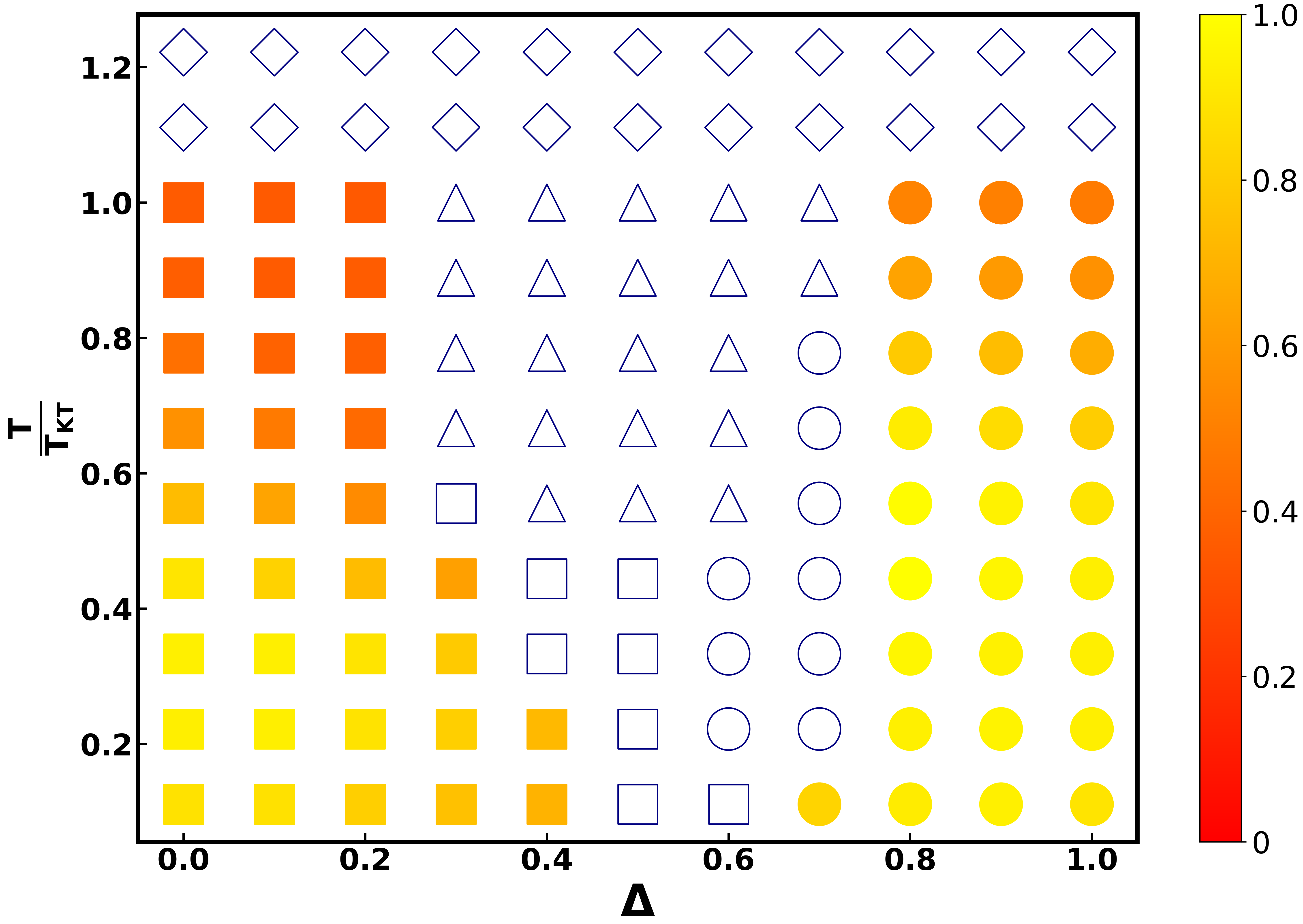
Figure 8: (color online) This diagram illustrates the Phase Diagram of the system, where distinct symbols are utilized to depict different phases, and their colors correspond to the associated exponent values as indicated by the color bar. Specifically, the symbols ‘circle’, ‘square’, ‘triangle’, and ‘diamond’ represent the Polar, Nematic, Coexistence, and Disordered phases, respectively. Within the Polar and Nematic regions, the filled symbols indicate sub-regions where the exponent can be calculated, while the unfilled symbols signify parameter values where the exponent calculation is not feasible. All other parameters remain consistent with those in fig.3.

IV Discussion

In this study, we investigate the attributes of a spin system situated on a 2D square lattice, where each spin has the flexibility to align within the range of $[0,2\pi]$. These spins engage with their immediate neighbors, and they possess the choice between ferromagnetic and nematic interactions, determined by a probability associated with the parameter $\Delta$. Employing the Markov chain Monte Carlo algorithm, we systematically explore the $(T,\Delta)$ space to gain insights into defect behaviors.
Our examination uncovers distinctive findings in different regions of the $(T,\Delta)$ plane, particularly within the context of mixed systems ($0<\Delta<1$). In the scenario of pure systems, where the parameter $\Delta$ takes on values of either 0 or 1, a distinct pattern emerges. As the temperature increases within the moderate to high range, without surpassing the critical temperature $T_{KT}$, the exponent governing the power-law decay of defect count experiences a reduction. This observation indicates a noteworthy trend: the rate at which defects are removed becomes slower in this temperature range. In contrast, at lower temperatures, the exponent remains close to 1. This dynamic gives rise to a significant transition as temperature changes. With increasing temperature, the system shifts from being predominantly influenced by the behavior of spin waves to being driven by the thermal dynamics of defects. In essence, there is a marked change in the dominant mechanisms that dictate the system’s behavior.

Furthermore, when examining mixed system—fascinating and intricate behaviors come to the forefront. For temperatures exceeding $T_{KT}$, disorder prevails regardless of the $\Delta$ value. However, for temperatures below $T_{KT}$, we discern three distinct regions: In proximity to the polar limit (small $\Delta$ values), the system primarily exhibits dominance of integer defects. Near the nematic limit (approaching $\Delta=1$), half-integer defects prevail. Around $\Delta\approx 0.50$, an intriguing coexistence region manifests, characterized by the simultaneous presence of integer and half-integer defects. These findings shed light on the complex interplay of temperature and interaction parameters, revealing diverse defect behaviors within the spin system.

V Acknowledgement

P.S.M., P.K.M. and S.M., thanks PARAM Shivay for computational facility under the National Supercomputing Mission, Government of India at the Indian Institute of Technology, Varanasi and the computational facility at I.I.T. (BHU) Varanasi. P.S.M. and P.K.M. thank UGC for research fellowship. S.M. thanks DST, SERB (INDIA), Project No.: CRG/2021/006945, MTR/2021/000438 for financial support.

References

- Mermin (1967) N. D. Mermin, Journal of Mathematical Physics 8, 1061 (1967).
- Hohenberg (1967) P. C. Hohenberg, Physical Review 158, 383 (1967).
- Mermin and Wagner (1966) N. D. Mermin and H. Wagner, Physical Review Letters 17, 1133 (1966).
- Chaikin and Lubensky (1995) P. M. Chaikin and T. C. Lubensky, Principles of Condensed Matter Physics (Cambridge University Press, 1995).
- Alba et al. (2009) V. Alba, A. Pelissetto, and E. Vicari, Journal of Physics A: Mathematical and Theoretical 42, 295001 (2009).
- Goldenfield (2018) N. Goldenfield, Lectures On Phase Transitions and THE Renormalization Group (Oxford University Press, 2018).
- Kosterlitz and Thouless (1973) J. M. Kosterlitz and D. J. Thouless, Journal of Physics C: Solid State Physics 6, 1181 (1973).
- Vanderstraeten et al. (2019) L. Vanderstraeten, B. Vanhecke, A. M. Läuchli, and F. Verstraete, Physical Review E 100, 062136 (2019).
- Mila (1993) F. Mila, Physical Review B 47, 442 (1993).
- Richter-Laskowska et al. (2018) M. Richter-Laskowska, H. Khan, N. Trivedi, and M. Maciej, Condensed Matter Physics 21, 33602 (2018).
- Jensen (2003) H. J. Jensen, Lecture Notes on Kosterlitz-Thouless Transition in the XY Model (2003).
- Packard (2013) D. Packard, University of Illinois at Urbana-Champaign, Loomis Laboratory of Physics, Physics 563, 1 (2013).
- Korshunov (1985) S. Korshunov, JETP Lett 41 (1985).
- Yurke et al. (1993) B. Yurke, A. N. Pargellis, T. Kovacs, and D. A. Huse, Phys. Rev. E 47, 1525 (1993).
- Lebwohl and Lasher (1972) P. A. Lebwohl and G. Lasher, Phys. Rev. A 6, 426 (1972).
- Tang and Selinger (2018) X. Tang and J. Selinger, Soft Matter 15 (2018), 10.1039/C8SM01901K.
- Carpenter and Chalker (1989) D. B. Carpenter and J. T. Chalker, Journal of Physics: Condensed Matter 1, 4907 (1989).
- Benakli and Granato (1997) M. Benakli and E. Granato, Physical Review B 55, 8361 (1997).
- Qin et al. (2009) M. Qin, X. Chen, and J.-M. Liu, Phys. Rev. B 80 (2009), 10.1103/PhysRevB.80.224415.
- Žukovič (2016) M. Žukovič, Phys. Rev. B 94, 014438 (2016).
- Park et al. (2008) J.-H. Park, S. Onoda, N. Nagaosa, and J. H. Han, Phys. Rev. Lett. 101, 167202 (2008).
- Maccari et al. (2020a) I. Maccari, N. Defenu, L. Benfatto, C. Castellani, and T. Enss, Phys. Rev. B 102, 104505 (2020a).
- Poderoso et al. (2011) F. C. Poderoso, J. J. Arenzon, and Y. Levin, Phys. Rev. Lett. 106, 067202 (2011).
- Lee and Grinstein (1985) D. H. Lee and G. Grinstein, Phys. Rev. Lett. 55, 541 (1985).
- Qi et al. (2013) K. Qi, M. Qin, X. Jia, and J.-M. Liu, Journal of Magnetism and Magnetic Materials 340, 127 (2013).
- Muzny and Clark (1992) C. D. Muzny and N. A. Clark, Physical review letters 68, 804 (1992).
- Pleiner (1988) H. Pleiner, Physical review letters 37 (1988).
- Jelić and Cugliandolo (2011) A. Jelić and L. F. Cugliandolo, 2011, P02032 (2011).
- Koo et al. (2006) K.-J. Koo, W.-B. Baek, B. Kim, and S. Lee, Journal of the Korean Physical Society 49 (2006).
- Maccari et al. (2020b) I. Maccari, N. Defenu, L. Benfatto, C. Castellani, and T. Enss, Phys. Rev. B 102, 104505 (2020b).
- De Gennes and Prost (1993) P.-G. De Gennes and J. Prost, The physics of liquid crystals, 83 (Oxford university press, 1993).
- Chandrasekhar (1992) S. Chandrasekhar, Liquid Crystals (Cambridge University Press, 1992).
- Priestly (2012) E. Priestly, Introduction to liquid crystals (Springer Science & Business Media, 2012).
- Hickl (2021) V. Hickl, Dynamics of topological defects in passive and active liquid crystals (2021).
- Chuang et al. (1991) I. Chuang, R. Durrer, N. Turok, and B. Yurke, Science 251, 1336 (1991).
- Harth and Stannarius (2020) K. Harth and R. Stannarius, Frontiers in Physics , 112 (2020).
- Note (1) In the mixed system, each spin possesses a finite probability of engaging in both ferromagnetic and nematic interactions. In the former case, spin orientation lies within the range of , while in the latter case, it spans over the range . Therefore, employing a color plot with a single colorbar to illustrate spin orientation is inappropriate in this context.