Early Planet Formation in Embedded Disks (eDisk) IX: High-resolution ALMA Observations of the Class 0 Protostar R CrA IRS5N and its surrounding

Abstract

We present high-resolution, high-sensitivity observations of the Class 0 protostar RCrA IRS5N as part of the Atacama Large Milimeter/submilimeter Array (ALMA) large program Early Planet Formation in Embedded Disks (eDisk). The 1.3 mm continuum emission reveals a flattened continuum structure around IRS5N, consistent with a protostellar disk in the early phases of evolution. The continuum emission appears smooth and shows no substructures. However, a brightness asymmetry is observed along the minor axis of the disk, suggesting the disk is optically and geometrically thick. We estimate the disk mass to be between 0.007 and 0.02 M_⊙. Furthermore, molecular emission has been detected from various species, including C¹⁸O (2–1), ¹²CO (2–1), ¹³CO (2–1), and H₂CO (3${}_{0,3}-2_{0,2}$, 3${}_{2,1}-2_{2,0}$, and 3${}_{2,2}-2_{2,1}$). By conducting a position-velocity analysis of the C¹⁸O (2–1) emission, we find that the disk of IRS5N exhibits characteristics consistent with Keplerian rotation around a central protostar with a mass of approximately 0.3 M_⊙. Additionally, we observe dust continuum emission from the nearby binary source, IRS5a/b. The emission in ¹²CO toward IRS5a/b seems to emanate from IRS5b and flow into IRS5a, suggesting material transport between their mutual orbits. The lack of a detected outflow and large-scale negatives in ¹²CO observed toward IRS5N suggests that much of the flux from IRS5N is being resolved out. Due to this substantial surrounding envelope, the central IRS5N protostar is expected to be significantly more massive in the future.

,

1 Introduction

Protostellar disks form as an outcome of the conservation of angular momentum during the gravitational collapse of the dust and gas in the envelope surrounding young stars (e.g., Terebey et al., 1984; McKee & Ostriker, 2007). These disks not only regulate the mass accreted onto the protostar but also provide the necessary ingredients for planet formation (Testi et al., 2014). Recent Atacama Large Milimeter/submilimeter Array (ALMA) observations with high spatial resolution have discovered that substructures such as gaps and rings are common in the dust emission of Class II young stellar object disks (ALMA Partnership et al., 2015; Andrews et al., 2018; Cieza et al., 2021). While these structures can be attributed to features such as snowlines and dust traps (Zhang et al., 2015; Gonzalez et al., 2017), they are largely thought to be indications of embedded planets (Dong et al., 2015; Zhang et al., 2018). The direct imaging of possible protoplanets in the gap of the continuum emission of the protostar PDS 70 further supports this idea (Keppler et al., 2018; Isella et al., 2019; Benisty et al., 2021).

Recent studies have shown that the mass reservoir of Class II disks is generally insufficient to form giant planets (Tychoniec et al., 2020). This suggests that planet formation is already well underway by the time a protostar reaches the Class II (T Tauri) phase. Interferometric observations over the last decade have shown that protostellar disks can be found in younger Class 0/I protostars (e.g., Tobin et al., 2012; Brinch & Jørgensen, 2013; Ohashi et al., 2014; Sheehan & Eisner, 2017; Sharma et al., 2020; Tobin et al., 2020). These disks are generally found to be larger and possibly more turbulent compared to disks around more evolved sources (Sheehan & Eisner, 2017; Tychoniec et al., 2020). Furthermore, evidence of substructures has been observed in a handful of embedded Class I sources (e.g., Sheehan & Eisner, 2017; Segura-Cox et al., 2020; Sheehan et al., 2020). These results, combined with the ubiquity of substructures in Class II disks, suggest that planet formation likely begins earlier during the Class 0/I phase when the disk is still embedded in its natal envelope.

To constrain how and when substructures form in young ($\lesssim$1 Myr old) protostellar disks and ultimately understand their nature, a sample of 19 nearby Class 0/I protostellar systems have been studied with ALMA as part of the Large Program Early Planet Formation in Embedded Disks (eDisk; Ohashi et al., 2023). One of these deeply embedded protostars located in the R Coronae Australis (R CrA) region, the most active star formation region in the Corona Australis molecular cloud, is the Class 0 source RCrA IRS5N (hereafter IRS5N; Harju et al. 1993; Chini et al. 2003). IRS5N (also referred to as CrA-20; Peterson et al., 2011) is part of a group of a dozen deeply embedded young stellar objects (YSOs) in a cluster dubbed the Coronet in the R CrA region (Taylor & Storey, 1984). Traditionally, the cluster is estimated to be at a distance of $\sim$ 130 pc. However, from the recent Gaia DR2 parallax measurements, the distance to the cluster has been updated to 147 $\pm$ 5 pc (Zucker et al., 2020), which we have adopted for this paper. This value is consistent with the distance of 149.4 $\pm$ 0.4 pc measured recently by Galli et al. (2020).

The Coronet has been extensively observed from X-rays to radio wavelengths (e.g., Peterson et al., 2011; Lindberg et al., 2014; Sandell et al., 2021, see also review by Neuhäuser & Forbrich 2008). Based on Spitzer photometry of the Coronet, IRS5N was first classified as a Class I source (Peterson et al., 2011), which was later updated to Class 0 with the addition of Herschel and JCMT/SCUBA data (Lindberg et al., 2014). From a recent reanalysis of the spectral energy distribution (SED) of IRS5N utilizing the most recent photometry and the updated Gaia distance above, we find its bolometric temperature ($T_{\mathrm{bol}}$) = 59 K and its bolometric luminosity ($L_{\mathrm{bol}}$) = 1.40 $L_{\odot}$ (Ohashi et al., 2023). Up to now, the highest angular resolution observations of IRS5N at submillimeter wavelengths so far were from the Submillimeter Array (SMA) in the compact configuration at a resolution of 4$.\!\!^{\prime\prime}$6 $\times$ 2$.\!\!^{\prime\prime}$6 (Peterson et al., 2011). In this paper, part of the series of first-look papers from eDisk, we present the first high-angular resolution ($\sim$0$.\!\!^{\prime\prime}$05), high-sensitivity continuum and spectral line observations toward IRS5N using ALMA. The field-of-view of our ALMA observations of IRS5N also captures the nearby binary protostar, IRS5 a and b. IRS5 (also known as R CrA 19; Peterson et al. (2011)) was first reported in Taylor & Storey (1984) and later found to be a binary (Chen & Graham, 1993; Nisini et al., 2005).

The paper is structured as follows: The observations and the data reduction process are described in Sect. 2. The empirical results from the observations of the disk continuum and the molecular line emission are presented in Sect. 3. The implications of the results are discussed in Sect. 4 and the conclusions are presented in Sect. 5.

2 Observations and Data Reduction

IRS5N was observed as part of the eDisk ALMA large program (2019.1.00261.L, PI: N. Ohashi) in Band 6 at 1.3 mm wavelength. The short-baseline observations were conducted on 2021 May 4 and on 2021 May 15 for a total on-source time of $\sim$76 minutes. The long-baseline observations were made between 2021 August 18 and October 2 for a total on-source time of $\sim$256 minutes. The shortest and the longest projected baselines were 15 m and 11,615 m, respectively. Along with the continuum, molecular line emissions from ¹²CO, ¹³CO, C¹⁸O, SO, SiO, DCN, $c$-C₃H₂, H₂CO, CH₃OH, and DCN were also targeted. A detailed description of the observations along with the spectral setup, correlator setup, and calibration is provided in Ohashi et al. (2023).

The ALMA pipeline-calibrated long- and short-baseline data were further reduced and imaged using the Common Astronomy Software Application (CASA) 6.2.1 (McMullin et al., 2007). The source position was estimated by calculating the continuum peak position for each execution block and aligned to a single phase center when calculating the scaling between the execution blocks. The self-calibration was carried out using the native phase centers of the observations. The short-baseline data were initially self-calibrated with six rounds of phase-only calibration followed by three rounds of phase and amplitude calibration. Then, the long-baseline data were combined with the self-calibrated short-baseline data, and four more rounds of phase-only calibration were performed on the combined data. The solutions of the continuum self-calibration are applied to the spectral line data as well.

The final continuum images were created with a range of robust parameters from -2.0 to 2.0. We adopt the robust value of 0.5 for the continuum image in this paper, providing a balance between sensitivity and resolution. This resulted in a synthesized beam of $0\hbox{$.\!\!^{\prime\prime}$}052\times 0\hbox{$.\!\!^{\prime\prime}$}035$ and an rms noise of 16 $\mu$Jy beam^-1. The spectral line images are created with robust parameters of 0.5 and 2.0 with uvtaper = 2000 k$\lambda$. We adopt robust 0.5 for most of the spectral lines except for the ¹³CO and H₂CO lines, where we adopt robust 2.0 to increase the signal-to-noise ratio. The details of the continuum observations and the detected spectral lines are summarized in Table 1.

Table 1: Overview of the continuum and the detected molecular lines

Continuum/Molecules	Transition	robust	Frequency	Beam	P.A.	$\Delta v$	RMS
			(GHz)	($\ \!\!{}^{\prime\prime}$)	(∘)	(km s-1)	(mJy beam-1)
Continuum	–	0.5	225.000000	0.05 $\times$ 0.03	60	–	0.016
C18O	$J=$ 2–1	0.5	219.560354	0.11 $\times$ 0.08	83.8	0.167	1.636
12CO	$J=$ 2–1	0.5	230.538000	0.11 $\times$ 0.08	85.9	0.635	0.987
13CO	$J=$ 2–1	2.0	220.398684	0.15 $\times$ 0.11	-87.3	0.167	2.104
H2CO	$J_{K_{a},K_{c}}=$ 3${}_{0,3}-2_{0,2}$	2.0	218.222192	0.14 $\times$ 0.11	-86.6	1.34	0.499
H2CO	$J_{K_{a},K_{c}}=$ 3${}_{2,1}-2_{2,0}$	2.0	218.760066	0.15 $\times$ 0.11	-86.8	0.167	1.471
H2CO	$J_{K_{a},K_{c}}=$ 3${}_{2,2}-2_{2,1}$	2.0	218.475632	0.17 $\times$ 0.13	-86.6	1.34	0.529

3 Results

3.1 Dust continuum emission

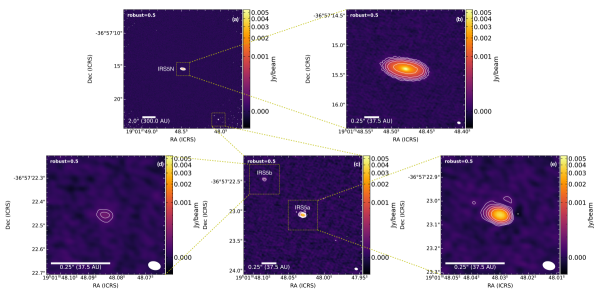
Figure 1: (a) 1.3 mm continuum images of R CrA IRS5N and IRS5 sources with a robust paramater of 0.5. (b) Zoomed-in view of the IRS5N disk. (c) Zoomed-in view of IRS5a and its companion IRS5b. (d) and (e) show further zoomed-in views of the individual sources of the IRS5 binary. The contour levels are 5$\sigma$, 10$\sigma$, 20$\sigma$, 40$\sigma$, and 80$\sigma$ with $\sigma=0.016$ mJy beam^-1. The synthesized beam is shown in white in the bottom right corner with a beam size of $0\hbox{$.\!\!^{\prime\prime}$}052\times 0\hbox{$.\!\!^{\prime\prime}$}035$ and a position angle of 75.4^∘. The color stretch used for the images is arcsinh to cover the dynamic range between the sources.

Figure 1 shows the continuum images from the ALMA data at 1.3 mm. Figure 1(a) displays the large-scale view of the continuum emission from the region, and the remaining panels show the zoom-in of the IRS5N and the IRS5 protostars.

Figure 1(b) shows the zoomed-in view of the IRS5N continuum image. The image shows a well-resolved flattened dust structure, which likely traces the disk surrounding the central protostar. The brightest emission of the disk is concentrated at its geometrical center with a peak intensity of 5.53 mJy beam^-1 as measured from the emission map corresponding to a brightness temperature of $\sim$94 K, calculated with the full Planck function. The brightness temperature of 94 K is relatively high for a protostar with $L_{bol}$ = 1.4 $L_{\odot}$ and deviates from the traditional assumptions of protostars generally derived from Class II disks (Kusaka et al., 1970; Chiang & Goldreich, 1997; Huang et al., 2018). One likely explanation for this high-brightness temperature is that IRS5N experiences self-heating through accretion luminosity, which has also been seen on other eDisk sources and further explored in Takakuwa et al. (in prep.). The total integrated flux density of IRS5N is 101 mJy, measured by integrating pixels where intensity is above 3$\sigma$. The geometrical peak position of IRS5N is $19^{\mathrm{h}}01^{\mathrm{m}}48\fs 48$, $-36^{\circ}57^{\prime}15\hbox{$.\!\!^{\prime\prime}$}39$. The full width at half maximum (FWHM) of IRS5N is estimated to be $\sim$62 au from the Gaussian fit model of the continuum emission. The deconvolved size enables us to estimate the inclination, $i$, of the IRS5N disk to be $\sim$65^∘ calculated from $i=\arccos(\theta_{\rm min}/\theta_{\rm maj})$, where $\theta_{\rm min}$ and $\theta_{\rm max}$ are the FWHM of the minor and major axes respectively.

Figure 1(c) shows the zoomed-in view of the binary source IRS5, with panels (d) and (e) showing the zoom-in of IRS5b and IRS5a, respectively. Nisini et al. (2005) first reported a separation of $\sim 0\hbox{$.\!\!^{\prime\prime}$}6$ between the two components based on pre-images with a relatively coarse pixel size of 0.14 arcsec/pixel. The pre-images were taken as part of preparations for spectroscopic observations using the ISAAC instrument of the Very Large Telescope (VLT). Our current high-resolution ALMA observations reveal that IRS5a and IRS5b have a projected separation of $\sim$0$.\!\!^{\prime\prime}$9 ($\sim$132 au at a distance of 147 pc). This difference between the previous and the new separation may be due to a combination of the proper motions of the sources, and the confusion from the scattered light in the infrared observations. The peak position of IRS5a as measured with Gaussian fitting is $19^{\mathrm{h}}01^{\mathrm{m}}48\fs 030$, $-36^{\circ}57^{\prime}23\hbox{$.\!\!^{\prime\prime}$}06$. We adopt this position as the coordinate of IRS5a. IRS5a is peaked at the center with a peak intensity of 3.87 mJy beam^-1 or $\sim$62 K and a flux density of 4.85 mJy. The secondary source, IRS5b, is much smaller and fainter than IRS5a. The peak position of IRS5b as measured with Gaussian fitting is $19^{\mathrm{h}}01^{\mathrm{m}}48\fs 084$, $-36^{\circ}57^{\prime}22\hbox{$.\!\!^{\prime\prime}$}46$. It has a peak intensity of $\sim$0.20 mJy beam^-1 or $\sim$3 K and a flux density of 0.26 mJy. The flux density of IRS5 was also measured by integrating above the 3$\sigma$ level over a region surrounding the individual continuum sources. From our observations, IRS5a is marginally resolved whereas IRS5b is not resolved.

3.2 Disk and envelope masses

The dust continuum emission with ALMA can be used to estimate the mass of the total disk structure surrounding the sources. Assuming optically thin emission, well-mixed gas and dust, and isothermal dust emission, the dust mass can be derived from

$$\centering M_{\mathrm{dust}}=\frac{D^{2}F_{\lambda}}{\kappa_{\lambda}B_{\lambda}(T_{\mathrm{dust}})},\@add@centering$$ (1)

where $D$ is the distance to the source ($\sim$147 pc) and $T_{\mathrm{dust}}$ is the temperature of the disk. $F{{}_{\lambda}}$, $\kappa_{\lambda}$, and $B_{\lambda}$ are the flux density of the disk, dust opacity, and the Planck function at the wavelength $\lambda$, respectively. Typically, for Class II disks, $T_{\mathrm{dust}}$ is often taken to be a fixed temperature of 20 K independent of the total luminosity (e.g., Andrews & Williams, 2005; Ansdell et al., 2016). However, for younger, more embedded Class 0/I disks, Tobin et al. (2020) found through radiative transfer modeling that the dust temperature scales as

$$\centering T_{\mathrm{dust}}\approx\mathrm{43K}\left(\frac{L_{bol}}{1L_{\odot}}\right)^{0.25},\@add@centering$$ (2)

For IRS5N with a bolometric luminosity of 1.40 $L_{\odot}$ Equation (2) yields $T_{\mathrm{dust}}$ = 47 K.

We estimate the disk masses using both dust temperatures. We adopt $\kappa_{\mathrm{1.3mm}}$ = 2.30 cm² g^-1 from dust opacity models of Beckwith et al. (1990) and assume a canonical gas-to-dust ratio of 100:1 to calculate disk masses using Equation (1). The resulting total disk mass for IRS5N is 0.019 $M_{\odot}$ for a dust temperature of 20 K and 6.65 $\times$ 10^-3 $M_{\odot}$ for a dust temperature of 47 K. The scaled dust temperature of IRS5a is similar to that of IRS5N, as Lindberg et al. (2014) found $L_{\mathrm{bol}}$ of IRS5a to be 1.7 $L_{\odot}$. Disk masses are also derived for the binary, IRS5. The estimated disk masses for all the continuum sources are presented in Table 2. It is important to note that the disk masses calculated using Equation (1) represent lower limits, as the continuum emission is most likely optically thick (see Section 4).

Table 2: Estimated disk masses of continuum emission sources.

Source	Flux Density	Gas+Dust Mass
		20 K	47 K
	(mJy)	($M_{\odot}$)	($M_{\odot}$)
IRS5N	100.65	0.019	6.65 $\times$ 10-3
IRS5a	4.85	8.92 $\times$ 10-4	3.20 $\times$ 10-4
IRS5b	0.26	4.73 $\times$ 10-5	–

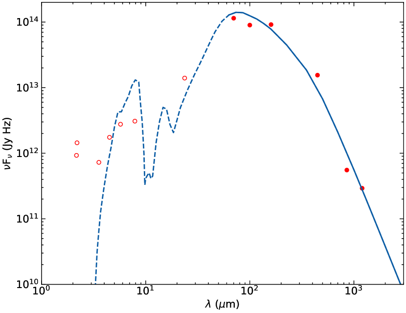
Figure 2: Fitting of the SED of IRS5N with a 1D radiative transfer model. Filled red circles represent SED values over 60 $\mu$m which are fitted by the model. Open red circles represent the remaining SED values used as input. The solid blue line represents the fit given by the model. The dashed blue line represents that the model does not fit this part of the SED.

For comparison, we estimate the mass of the envelope around IRS5N using a simple 1D dust radiative transfer model. We adopt a single power-law density profile, $n\propto r^{-1.5}$ corresponding to material in free-fall between inner and outer radii of 100 and 10,000 au, respectively, and take the bolometric luminosity of the source determined from the full SED as the sole (internal) heating source of the dust. The dust radiative transfer model then calculates the temperature-profile of the dust in the envelope self-consistently and predicts the SED of the resulting source emission. To constrain the envelope mass we then fit the long wavelength ($\lambda>60$ $\mu$m) part of the spectral energy distribution of IRS5N. This method allows for a slightly more robust way of determining the envelope mass than simply adopting a single submilimeter flux point and isothermal dust as it provides an estimate of the temperature of the dust taking into account the source luminosity (e.g., Jørgensen et al., 2002; Kristensen et al., 2012). The resulting fit of the envelope model is shown in Fig. 2 with the envelope mass constrained to be 1.2 $M_{\odot}$. The estimated uncertainty on the fitted envelope mass is comparable to the flux calibration uncertainty, typically about 20% for the measurements used here. However, systematic uncertainties of the adopted simplified physical structure of the envelope and the dust opacity laws will likely dominate over this. It is worth emphasizing that this simplified model is not expected to, and does not, fit the emission at wavelengths shorter than 60 $\mu$m due to the complex geometry of the system at small scales and contributions from scattering.

3.3 Molecular lines

Among the molecules mentioned in Section 2, emission is detected in C¹⁸O, ¹²CO, ¹³CO, and H₂CO molecules in our observations. Figure 3 presents an overview of the integrated-intensity (moment-0) and mean-velocity (moment-1) maps of all the detected molecules toward IRS5N and IRS5. The moment 1 maps were generated by integrating the regions where $I_{\nu}\geq 3\sigma$, where $\sigma$ is the rms per channel. The maps for C¹⁸O and ¹²CO were made using a robust parameter of 0.5, while the maps for the remaining molecules were made using a robust parameter of 2.0. The channel maps of all the observed molecules around IRS5N are shown in Appendix A.

It is worth emphasizing that large-scale negative components are visible in the channel maps of the molecules, particularly of the CO isotopologues. These negative components indicate that a significant amount of extended flux originating from the large-scale structures surrounding the sources is being resolved out. While it is crucial to analyze these structures to build a comprehensive picture of the physics and chemistry of the system, we are constrained by the limitations of our high-resolution observations. The maximum recoverable scale, ($\theta_{MRS}$) of our observations was 2$.\!\!^{\prime\prime}$91. Hence, this study focuses only on small-scale structures, such as the disk and envelope of individual systems.

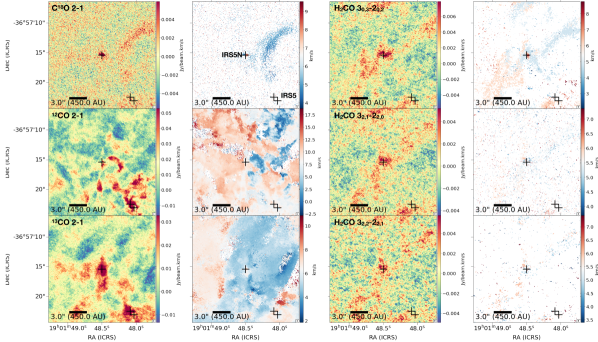
Figure 3: Overview of all the molecular lines detected towards IRS5N and IRS5. For each molecule, the moment 0 map is shown on the left and the moment 1 map is shown on the right. The cross marks show the peak of the continuum emission of IRS5N and the binary IRS5. The maps are created by integrating over the velocity ranges of 3.68 – 9.53 km s^-1, -5.38 – 20.65 km s^-1, 0.51 – 12.03 km s^-1, 2.06 – 8.76 km s^-1, 3.68 – 7.36 km s^-1, and 3.40 – 7.42 km s^-1 for C¹⁸O, ¹²CO, ¹³CO, H₂CO (3_0,3–$2_{0,2}$), H₂CO (3_2,1–$2_{2,0}$), and H₂CO (3_2,2–$2_{2,1}$) respectively.

The synthesized beam is shown in black at the bottom right corner of each image, enclosed by a square.

3.3.1 C¹⁸O

Figure 4 shows the zoomed-in integrated moment 0 and moment 1 maps of the C¹⁸O (2–1) emission around IRS5N. The moment 0 map shows a flattened structure along with a velocity gradient extended along the major axis of the disk, traced by the continuum emission. The size of the gas disk radius from the C¹⁸O emission is comparable to that of the disk continuum and has a hole at the protostar position. Based on the consistency between the C¹⁸O emission and the continuum emission, the radius of the disk can be assumed to be the same as the FWHM of the continuum, $\sim$62 au. The hole at the protostellar position has negative intensities below 3$\sigma$ at 5.35 km s^-1 – 6.02 km s^-1 (see Figure 13, 19). The deficit likely results from continuum over-subtraction due to the C¹⁸O emission being relatively weak compared to the bright continuum emission.

The moment 1 map of the C¹⁸O emission shows that the blue- and the red-shifted velocities have a distinct separation along the eastern and western sides, respectively. Such a velocity profile is consistent with a rotating disk. The position-velocity (PV) analysis of the C¹⁸O emission is presented in Section 4.

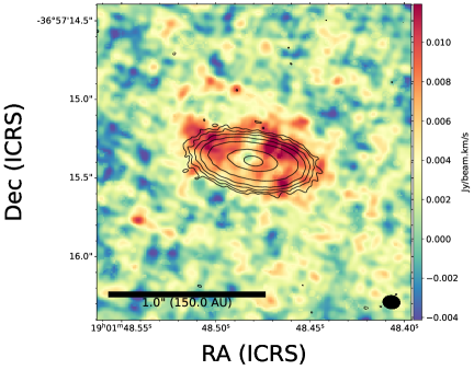
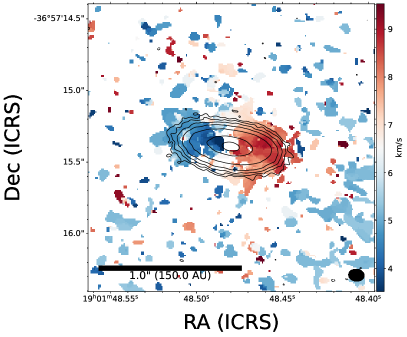
Figure 4: Zoomed-in moment 0 map (left) and moment 1 map (right) of the C¹⁸O ($J$=2–1) emission towards IRS5N created with the robust value of 0.5. The overlaid contours show continuum emission from 3$\sigma$ to 192$\sigma$, with each contour doubling the previous $\sigma$ level. The maps are created by integrating over the velocity ranges of 3.68 – 9.53 km s^-1. The synthesized beam size for the C¹⁸O emission is 0$.\!\!^{\prime\prime}$11 $\times$ 0$.\!\!^{\prime\prime}$08.

3.3.2 ¹²CO and ¹³CO

Figure 5: Zoomed-in moment 0 (left) and moment 1 (right) maps of ¹²CO (top) and ¹³CO (bottom) emission. The maps are created by integrating over the velocity ranges of -5.38 – 20.65 km s^-1 and 0.51 – 12.03 km s^-1 for ¹²CO and ¹³CO , respectively. The cross represents the peak position of the IRS5N continuum. Synthesized beam is shown in black at the bottom right corner of each image.

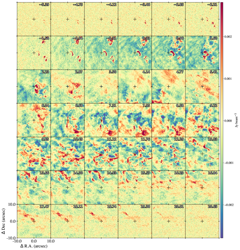
Figure 14: Same as Figure 13 but for ¹²CO (2–1) instead.

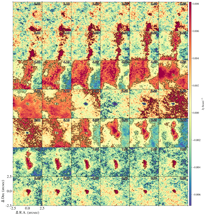
Figure 21: Same as Figure 19 but for ¹³CO (2–1) instead.

Figure 5 shows zoomed-in moment 0 and moment 1 maps of ¹²CO (2–1) and ¹³CO (2–1) emission near IRS5N. While the ¹²CO emission shows extended emission around IRS5N, it does not seem to trace any obvious outflow/jet associated with the protostar, which is puzzling. The spiral structure seen towards the west of the protostar is blue-shifted and seems to trace infalling material onto the protostellar disk (see channel maps; Figure 14). Additionally, extended emission is seen in the surrounding of IRS5N, some of which likely originates from the protostar. In contrast, the ¹³CO plot shows some emission in the north-south direction of the protostar but this emission is mostly observed in red-shifted velocity channels (Figure 21). The channel maps of ¹³CO also show an apparent deficit near the protostellar position at the velocity range of 5.02 km s^-1 – 6.19 km s^-1 which is much more prominent than the deficit seen on the C¹⁸O channel maps (Figure 19). This is most likely due to the continuum over-subtraction, similar to that of the C¹⁸O emission. This suggests that the ¹³CO emission is extended and somewhat optically thick, leading it to become resolved-out as $\theta_{MRS}$ = 2$.\!\!^{\prime\prime}$91. The moment maps of ¹²CO and ¹³CO reveal the complex nature of the emission around IRS5N.

We also detected molecular emission in ¹²CO (2–1) and ¹³CO (2–1) towards IRS5. Figure 6 (a) shows the moment 0 maps of ¹²CO emission around IRS5a and IRS5b. The ¹²CO emission around IRS5a is compact, with no visible outflow structure. In contrast, bright, elongated emission is observed toward IRS5b in the east-west direction, possibly tracing an outflow from IRS5b. The emission has a velocity gradient and relatively high velocities from -1.58 km s^-1 – 2.23 km s^-1 and 9.85 km s^-1 – 13.03 km s^-1 as shown in the ¹²CO channel maps in Figure 7. Additionally, bright extended emission is also seen around IRS5b which connects its way into IRS5a. Based on the ¹²CO emission towards the IRS5 binary, we estimate its systemic velocity to be $\sim$6.50 km s^-1. The channel maps show that the blue-shifted emission seems to emanate from IRS5b and stream onto IRS5a as the velocity increases. Similar stream- or bridge-like features are observed toward other protostellar binaries (e.g., Sadavoy et al., 2018; van der Wiel et al., 2019; Jørgensen et al., 2022) and may trace transport of material between the companions triggered by interactions during their mutual orbits (e.g., Kuffmeier et al., 2019; Jørgensen et al., 2022). The streaming emission appears to end in a disk-like structure around IRS5a, seen in channel maps of 6.68 km s^-1 – 9.85 km s^-1. Notably, this structure is much larger than the observed size of the dust continuum structure of IRS5a seen in Figure 1, indicating it likely traces the inner envelope surrounding the disk. Additionally, in channel maps ranging from 7.31 km s^-1 to 8.58 km s^-1, extended emission possibly tracing an outflow is seen towards the southeast of IRS5a. Conversely, the ¹³CO emission in Figure 6 (b) traces the extended mutual envelope material surrounding both sources. The emission is much brighter towards IRS5b than IRS5a, with the brightness peak towards the southwest of IRS5b.

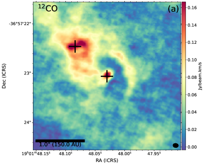
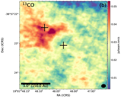
Figure 6: Zoomed-in moment 0 maps of ¹²CO emission (a) around the IRS5 binary source and ¹³CO emission (b) around the IRS5 binary source. The crosses represent the peak position of the continuum emission of IRS5a and IRS5b sources. The maps are created by integrating over the velocity ranges of -4.75–14.93 km s^-1 and 2.85 – 9.86 km s^-1 for ¹²CO and ¹³CO , respectively. Synthesized beam is shown in black at the bottom right corner of each image.

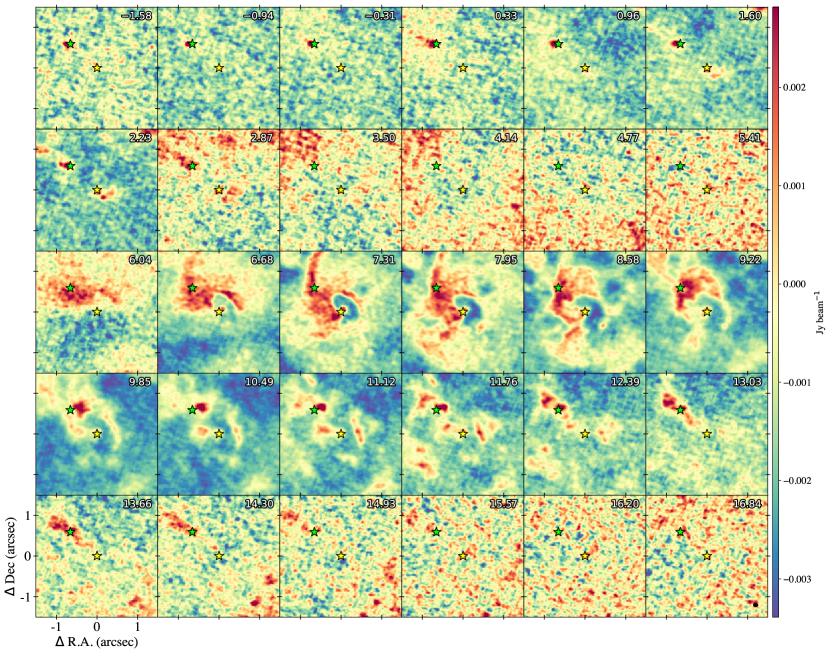
Figure 7: Channel maps showing the ¹²CO emission around the two sources of the IRS5 system. The yellow star and the green star show the peak position of the continuum emission of IRS5a and IRS5b, respectively. The numbers at the top show the corresponding velocity of each channel map. Synthesized beam is shown in black at the bottom right corner of the final channel map.

3.3.3 H₂CO

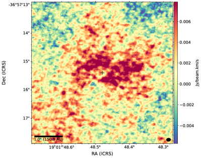
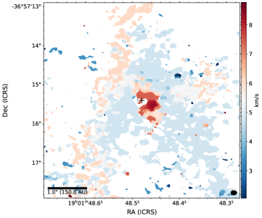
Figure 8: Same as Figure 5 but for H₂CO (3_0,3–$2_{0,2}$) instead. The maps are created by integrating over the velocity ranges of 2.06 – 8.76 km s^-1.

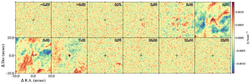
Figure 16: Same as Figure 13 but for H₂CO (3_0,3–2_0,2) instead.

In addition to the CO isotopologues, we also detect emission from three H₂CO lines towards IRS5N. Figure 3 shows that the emission structure of the three transitions are similar to one another, with most of the emission surrounding the disk and inner envelope with extended emission towards the northwest and southeast direction of the source. There is a slight velocity difference between the two sides of the extended source as shown by the moment 1 maps. The 3_0,3–$2_{0,2}$ transition has the lowest upper-level energy and is also the strongest, as expected. A magnified view of the moment 0 and moment 1 maps of the brightest transition of H₂CO, $3_{0,3}$–2_0,2, is shown in Figure 8. The zoomed-in maps reveal that besides the large-scale emission, some red-shifted emission is visible towards the west of the disk, similar to that of the C¹⁸O emission (see Figure 4), but appears to lack the corresponding blue-shifted counterpart, suggesting asymmetric distribution of the chemical composition of the disk/envelope system.The velocity channel maps show that there is negative emission at the position of the protostar which again is likely caused by continuum over-subtraction (see Figure 16, 22). However, the large-scale negatives seen in the velocity channel maps suggest that a significant amount of flux is getting resolved out.

4 Analysis and Discussion

4.1 Continuum Modeling

As shown in Figure 1, even though we sufficiently resolve the disk of IRS5N, no apparent substructures can be identified in the continuum emission. IRS5a also appear to be relatively smooth, while IRS5b is not resolved.

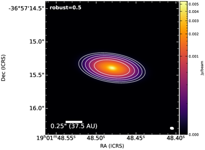
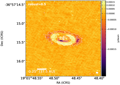
Figure 9: IRS5N disk model (left) and residual (right) created using double Gaussian components. Contours show the 3$\sigma$, 6$\sigma$, 12$\sigma$, 24$\sigma$ and 48$\sigma$. The dashed contours indicate negative intensity. The white ellipse on the bottom right corner of each image shows the synthesized beam.

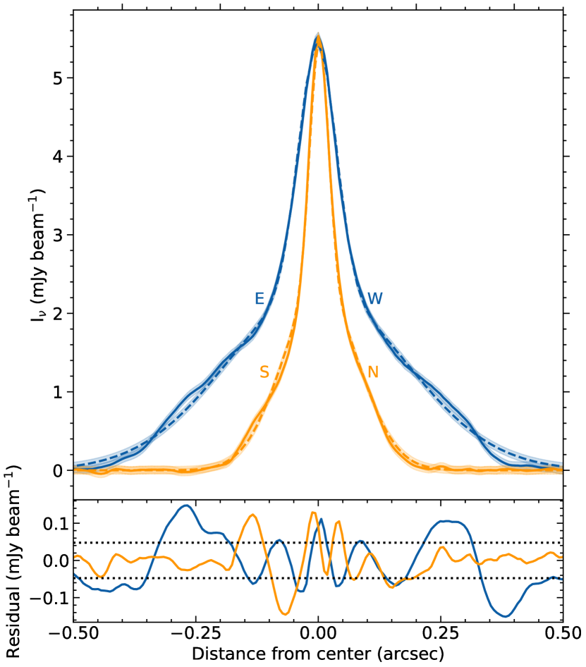
Figure 10: Intensity profiles of the 1.3 mm continuum emission of IRS5N shown in Figure 1(b) and double Gaussian component model shown in Figure 9. The solid line represents the observed emission and the dashed line represents the model. The blue lines indicate the intensity along the major axes and the orange lines represent the intensity along the minor axes. The smaller plot at the bottom shows the residual intensity after subtracting the model from the observation. The shaded region and the horizontal dotted lines indicate $\pm 3\sigma$ uncertainties with $\sigma=0.016$ mJy beam^-1.

Figure 9 shows the best-fit model and its corresponding residual of the continuum emission of IRS5N made with CASA task imfit. The model was created using two 2D Gaussian components as a single Gaussian model misses a lot of emission of the continuum. The residual image and the intensity plots in Figure 10 show that the double-component model is able to recover most of the continuum emission. The fitting results of both models are provided in Table 3. The parameters of the disk continuum such as its peak position, P.A., and $i$ do not change significantly between the two components of the model. It is important to note that the residuals are a result of the model not representing the structure of the emission and can not necessarily be taken as evidence of the presence of substructures in the distribution of material within the dusty disk. The residual image shows that there is some asymmetry in the direction of the minor axis (North-South). The disk appears to be brighter in the south compared to the north. Such asymmetry in the minor axis is observed in several eDisk sources (Ohashi et al., 2023). This can be attributed to the geometrical effects of optically thick emission and flaring of the disk (Takakuwa et al., in prep.). The north side of the disk is more obscured compared to the south which is expected to be on the far side of the disk with $i\sim 65^{\circ}$, where 90^∘ represents the completely edge-on case.

We also fit the continuum emission for both sources in the IRS5 system. Figure 11 shows the model and the residual created of IRS5a and IRS5b after subtracting a single 2D Gaussian. The model is able to reasonably capture the majority of the continuum emission from both sources as seen from the residual images. The results of the fitting are provided in Table 3.

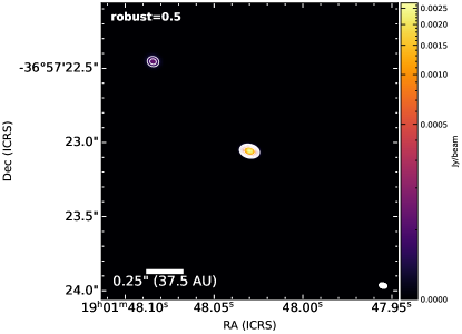
Figure 11: Same as Figure 10 but for IRS5a binary source with the model made with a single Gaussian peak for each continuum emission observed.

Table 3: Best-fit parameters.

Parameter	Single Gaussian Component			Double Gaussian Components
	IRS5N	IRS5a	IRS5b	IRS5N
				Component 1	Component 2
R.A (h:m:s)	19:01:48.480	19:01:48.030	19:01:48.084	19:01:48.480	19:01:48.480
Dec (d:m:s)	-36:57:15.39	-36:57:23.06	-36:57:22.46	-36:57:15.39	-36:57:15.39
Beam size ($\ \!\!{}^{\prime\prime}$)	0.05 $\times$ 0.03	0.05 $\times$ 0.03	0.05 $\times$ 0.03	0.05 $\times$ 0.03	0.05 $\times$ 0.03
Beam P.A. (∘)	75.44	75.44	75.44	75.44	75.44
$\theta_{\mathrm{maj}}$ (mas) †	373.7 $\pm$ 7.1	22.91 $\pm$ 0.95	46 $\pm$ 16	73.58 $\pm$ 1.69	423.9 $\pm$ 3.0
$\theta_{\mathrm{min}}$ (mas) †	156.7 $\pm$ 2.9	16.82 $\pm$ 0.56	40 $\pm$ 26	28.32 $\pm$ 0.76	179.4 $\pm$ 1.3
P.A. (∘) †	81.10 $\pm$ 0.76	84.7 $\pm$ 5.7	174 $\pm$ 54	81.22 $\pm$ 0.80	81.08 $\pm$ 0.29
Inclination (∘)	65.21 $\pm$ 0.70	42.76 $\pm$ 3.29	29.59 $\pm$ 74.38	67.36 $\pm$ 0.84	64.96 $\pm$ 0.27
Peak Intensity (mJy beam-1)	2.970 $\pm$ 0.054	3.893 $\pm$ 0.020	0.174 $\pm$ 0.00022	3.172 $\pm$ 0.039	2.286 $\pm$ 0.016
Flux Density (mJy)	99.1 $\pm$ 1.9	4.727 $\pm$ 0.041	0.361 $\pm$ 0.00063	7.09 $\pm$ 0.12	98.30 $\pm$ 0.69

Note. — $\dagger$ Values are deconvolved from the beam.

4.2 Kinematics of the disk: Position-velocity diagram

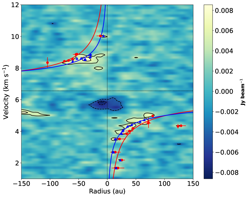
Figure 12: PV diagram of C¹⁸O emission towards IRS5N cut along its major axis. The points derived using the “edge” and “ridge” methods and their corresponding rotation curves are shown in blue and red, respectively. The black contours start at 3$\sigma$ level and increase every 2$\sigma$. Dashed contours show the corresponding negative contours.

The kinematics of the protostellar disk are investigated with position-velocity (PV) diagrams of molecular line emission that trace the disk. For IRS5N, C¹⁸O is the only molecule where evidence of rotation is seen in the protostellar disk (see Figure 3). C¹⁸O is much less optically thick and is a better disk tracer than other CO isotopologues, making it an excellent species for PV analysis. Figure 12 shows the PV diagram of IRS5N in C¹⁸O along the major axis of the disk. The PV diagram shows that the blue-shifted emission and the red-shifted emission are separated in the northeast and the southwest, respectively.

The PV diagram was fitted using the pvanalysis package of the Spectral Line Analysis/Modeling (SLAM) code (Aso & Sai, 2023) to investigate the nature of the rotation. The details of the fitting procedure are given in Ohashi et al. (2023), but a short description is provided here. The code determines the corresponding position at a given velocity using the PV diagram and calculates two types of representative points known as the edge and the ridge. The ridge is defined as the intensity-weighted mean calculated with emission detected above a given threshold, while the edge corresponds to the outermost contour defined by a given threshold. For the analysis of the PV diagram of the C¹⁸O emission around IRS5N, a threshold of $3\sigma$ level was used, where $\sigma=1.636$ mJy beam^-1. The edge and the ridge are then fit separately with a single power-law function given by

$$V_{\mathrm{rot}}=V_{b}\left(\frac{R}{R_{b}}\right)^{-p}+V_{sys},$$ (3)

where $V_{\mathrm{rot}}$ is the rotational velocity, $R_{b}$ is the break radius, $V_{b}$ is the rotational velocity at $R_{b}$, $p$ is the power-law index, and $V_{sys}$ is the systemic velocity of the system.

Table 4: PV fitting results for C¹⁸O with SLAM

Fitting method	Edge	Ridge
Rb (au)	76.98 $\pm$ 2.30	42.80 $\pm$ 0.44
$p_{\mathrm{in}}$	0.554 $\pm$ 0.047	0.379 $\pm$ 0.012
$v_{\mathrm{sys}}$ (km s-1)	6.564 $\pm$ 0.024	6.507 $\pm$ 0.008
Min ($M_{\odot}$)	0.398 $\pm$ 0.041	0.184 $\pm$ 0.008

The fitting results of the SLAM code are summarized in Table 4. Here, the ridge points are calculated using the 1D intensity weighted mean profile, called “mean” fitting method. However, the ridge points can also be calculated using the center of the Gaussian fitting. Using this “Gaussian” fitting method, we get R_b = 39.75 $\pm$ 0.76 au, $p_{\mathrm{in}}$ = 0.515 $\pm$ 0.029, $v_{\mathrm{sys}}$ = 6.464 $\pm$ 0.020 km s^-1, and M_in = 0.246 $\pm$ 0.015 ($M_{\odot}$), which are consistent to the values derived from the “mean” method. In the case of both the edge and ridge methods, the value of $p_{\mathrm{in}}$ is found to be close to 0.5, suggesting that the disk of IRS5N is already in Keplerian rotation. Typically, Keplerian rotation is commonly observed in more evolved sources (Simon et al., 2000). However, recent studies have found that some Class 0 sources already possess Keplerian disks (e.g. Tobin et al., 2012; Ohashi et al., 2014, 2023). In both the ridge and the edge methods, Keplerian rotation is observed out to a radius of $\sim$40 au and $\sim$76 au, respectively. The FWHM of the disk continuum falls well within this range, indicating that it could serve as a reliable indicator of the disk size of IRS5N. Under this assumption, the mass of the central source of IRS5N is estimated to be 0.398 $\pm$ 0.041 $M_{\odot}$ and 0.184 $\pm$ 0.008 $M_{\odot}$ for the edge and the ridge cases, respectively. The actual mass of the central source likely lies between these two estimates, approximately 0.3 $M_{\odot}$ (Maret et al., 2020). This shows that with a stellar mass of $\sim$0.3 $M_{\odot}$ compared to a disk mass of $\sim 0.007-0.02M_{\odot}$ and an envelope mass of 1.2 $M_{\odot}$, IRS5N is a deeply embedded protostar.

The stability of the disk against gravitational collapse can be estimated by using Toomre’s $Q$ parameter

$$\centering Q=\frac{c_{s}\Omega}{\pi G\Sigma},\@add@centering$$ (4)

where $c_{s}$ is the sound speed, $\Omega=GM_{*}/R^{3}$ is the differential rotation value of a Keplerian disk at the given radius $R$, $M_{*}$ is the mass of the protostar, $G$ is the gravitational constant, and $\Sigma$ is the surface density. A disk is considered gravitationally stable if $Q>1$, while $Q<1$ suggests that the disk may be prone to fragmentation. This equation can also be expressed in the form given by Kratter & Lodato (2016) and Tobin et al. (2016) as

$$\centering Q\approx 2\frac{M_{*}H}{M_{d}R},\@add@centering$$ (5)

where $H=c_{s}/\Omega$, $M_{d}$ is the mass of the disk, and $R$ is the radius of the disk. For IRS5N with $M_{*}$ = 0.3 $M_{\odot}$ and $R=62$ au, we find $Q\approx 3.5$ and 15 for disk masses of 0.019 $M_{\odot}$ and $6.65\times 10^{-3}M_{\odot}$ at 20 K and 47 K, respectively. This implies that the disk of IRS5N is gravitationally stable.

4.3 The low molecular emission around IRS5N

In Section 3, we mention that although we see extended emission in ¹²CO and ¹³CO in the region around IRS5N, we do not see any clear signs of outflow in these molecules. Emission is also not detected in SiO ($J$=5–4) or SO ($J$=6₅–5₄), both of which are known tracers of outflow and shocks (e.g., Schilke et al., 1997; Wakelam et al., 2005; Ohashi et al., 2014; Sakai et al., 2014). This is in contrast to most known young Class 0/I sources, where observations of a prominent outflow have become ubiquitous. Additionally, most of the emission detected in H₂CO, the only other molecule besides the CO isotopologues detected around IRS5N, is at a tentative level of 3$\sigma-5\sigma$.

The curious case of low emission around IRS5N has also been noted by previous studies (Nutter et al., 2005; Lindberg et al., 2014). Lindberg et al. (2014) specifically noted that only marginal residuals remained in the Herschel/PACS maps of the region when assuming that all emission originated from the IRS5 source. Recent studies suggest that previously thought young Class 0 objects exhibiting weak molecular line emission and lack prominent high-velocity outflow structures may actually be potential candidates for first hydrostatic core (FHSC) (Busch et al., 2020; Maureira et al., 2020; Dutta et al., 2022). These FHSC objects, however, have a relatively short lifetime of $\sim$10³ yr and simulations predict their luminosities to be $\sim$0.1 $L_{\odot}$ with the mass of the central source of $\lesssim$0.1 $M_{\odot}$ (Commerçon et al., 2012; Tomida et al., 2015; Maureira et al., 2020). Considering that IRS5N has a bolometric luminosity of 1.40 $L_{\odot}$ and a protostellar mass of 0.3 $M_{\odot}$, it has already progressed well beyond the FHSC stage and this most likely is not the explanation for the observed low emission and lack of outflow. Nonetheless, given the presence of a massive envelope of $\sim$1.2 $M_{\odot}$ surrounding IRS5N, it is likely to become much more massive in the future.

The peculiarity of the molecular emission characteristics of IRS5N are most likely explained by the complexity of the Coronet region. IRS7B, another YSO source of eDisk from the Coronet region, also seems to lack an outflow in the spectral lines (Ohashi et al., 2023). The Coronet hosts numerous YSOs and Molecular Hydrogen emission-line Objects (MHOs) with more than 20 Herbig-Haro (HH) objects (see Wang et al., 2004, and references therein). Such an environment might be affecting the molecular emission seen from these sources. ¹²CO, being optically thick, is the most affected. We do observe ¹³CO emission in the North-South direction of the source, roughly in the direction where the outflow is expected. However, this is only seen at low velocity, red-shifted channel maps. C¹⁸O appears to be the least affected among the CO isotopologues as it is the most optically thin of the three and is not as hidden behind the optically thick emission from the cloud like ¹²CO and ¹³CO making it mostly sensitive to the inner disk where the CO is evaporated from the dust grains (Jørgensen et al., 2015).

5 Conclusions

We have presented high-resolution, high-sensitivity observations of the protostar IRS5N and its surroundings as part of the eDisk ALMA Large program. Our ALMA band 6 observation had a continuum angular resolution of $\sim 0\hbox{$.\!\!^{\prime\prime}$}05$ ($\sim$8 au) and molecular line emission from C¹⁸O, ¹²CO, ¹³CO, and H₂CO. The main results of the paper are as follows:

1. The 1.3 mm dust continuum emission traces protostellar disks around IRS5N and IRS5. The continuum emissions appear smooth, with no apparent substructures in either source. However, the disk of IRS5N shows brightness asymmetry in the minor axis, with the southern region appearing brighter than the northern region. The asymmetry can be attributed to the geometrical effects of optically thick emission and flaring of the disk.

2. IRS5N has a disk radius of $\sim$62 au elongated along the northeast to southwest direction with a P.A. of 81.10^∘. IRS5a has a much smaller disk radius of $\sim$13 au with a P.A. of $\sim$85^∘. The disk of IRS5b remains unresolved. Using the total integrated intensity of each source and assuming a temperature of $T=20$ K, which is a typical dust temperature for Class II disks, the estimated disk masses for IRS5N, IRS5a, and IRS5b are 0.02, 9.18 $\times$ 10^-4, and 6.48 $\times$ 10^-5 $M_{\odot}$, respectively. At a temperature of $T=47$ K based on radiative transfer, the estimated disk masses for IRS5N and IRS5a are 6.65 $\times$ 10^-3 and 3.20 $\times$ 10^-4 $M_{\odot}$, respectively.

3. Disk rotation is observed in the C¹⁸O emission around IRS5N, with the blue- and red-shifted emission separated along the major axis of the disk. PV analysis of the emission reveals the disk is in Keplerian rotation. The stellar mass of the central source of IRS5N is estimated to be $\sim$0.3 $M_{\odot}$.

4. Using a 1D dust radiative transfer model, the estimated envelope mass around IRS5N is 1.2 $M_{\odot}$. The envelope mass is much greater than the disk mass of 0.02 $M_{\odot}$ and stellar mass of 0.3 $M_{\odot}$ indicating IRS5N is a highly embedded protostar.

5. The ¹²CO and ¹³CO maps towards IRS5N are complex and lack any apparent indication of an outflow or cavity. In contrast, the ¹²CO maps around IRS5 show emission streaming from IRS5b to IRS5a, tracing the gas connecting to the disk-like structure around the latter. This observation potentially suggests material transport between the two sources.

Appendix A Channel maps

Figure 13–18 show the selected large-scale channel maps of ¹²CO, ¹³CO, C¹⁸O, and H₂CO emission observed toward IRS5N. Figure 19–24 show the zoomed-in view of the molecular emissions observed.

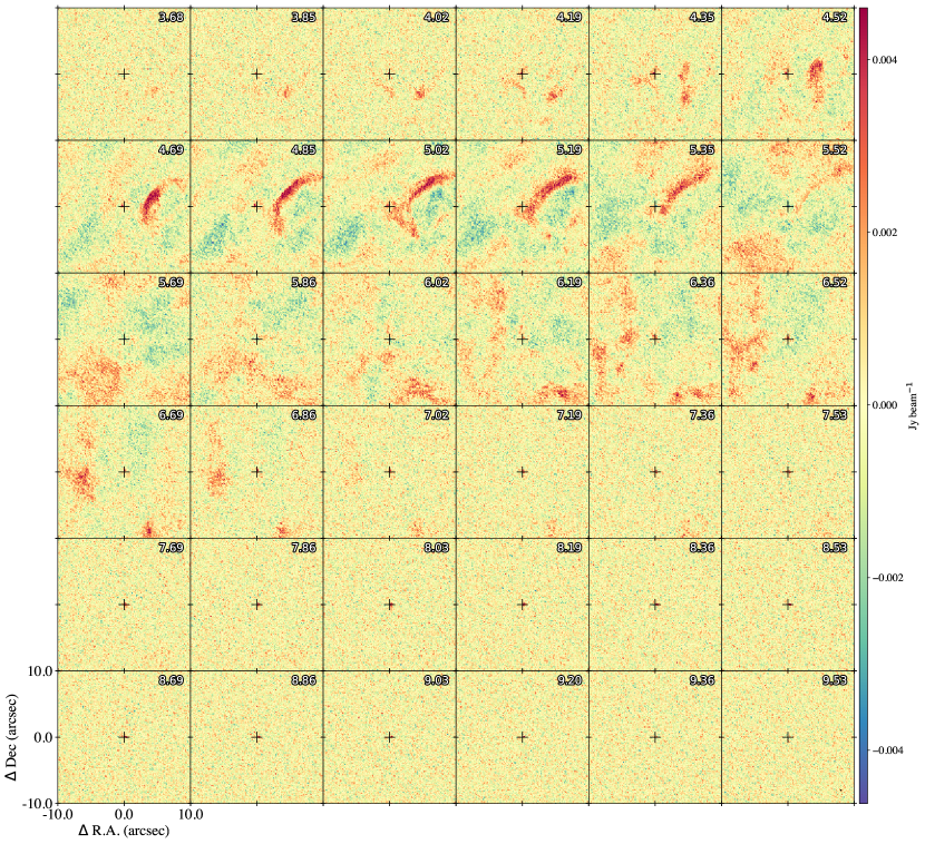
Figure 13: Selected channel maps showing the C¹⁸O (2–1) emission around IRS5N. The numbers at the top show the corresponding velocity of each channel map. The cross shows the peak position of the IRS5N continuum. Synthesized beam is shown in black on the bottom right corner of the final channel.

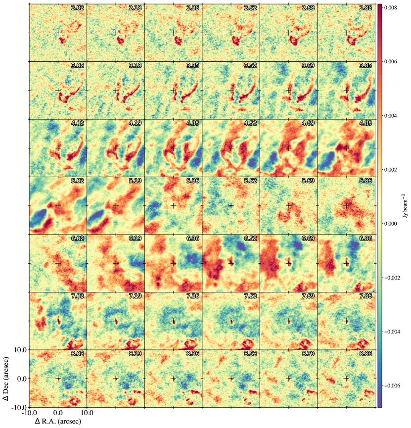
Figure 15: Same as Figure 13 but for ¹³CO (2–1) instead.

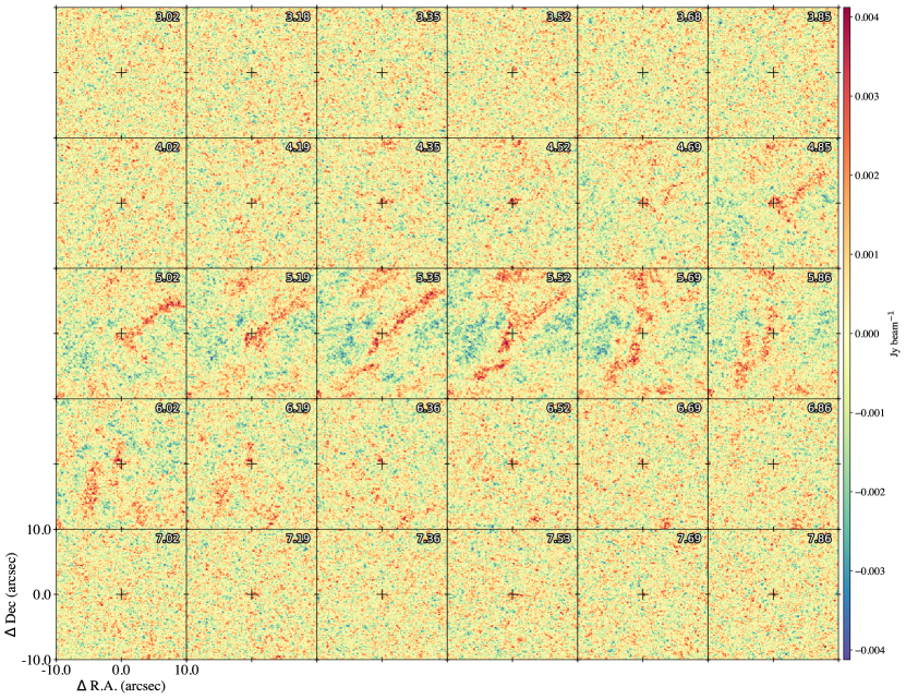
Figure 17: Same as Figure 13 but for H₂CO (3_2,1–2_2,0) instead.

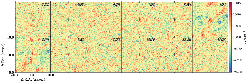
Figure 18: Same as Figure 13 but for H₂CO (3_2,2–2_2,1) instead.

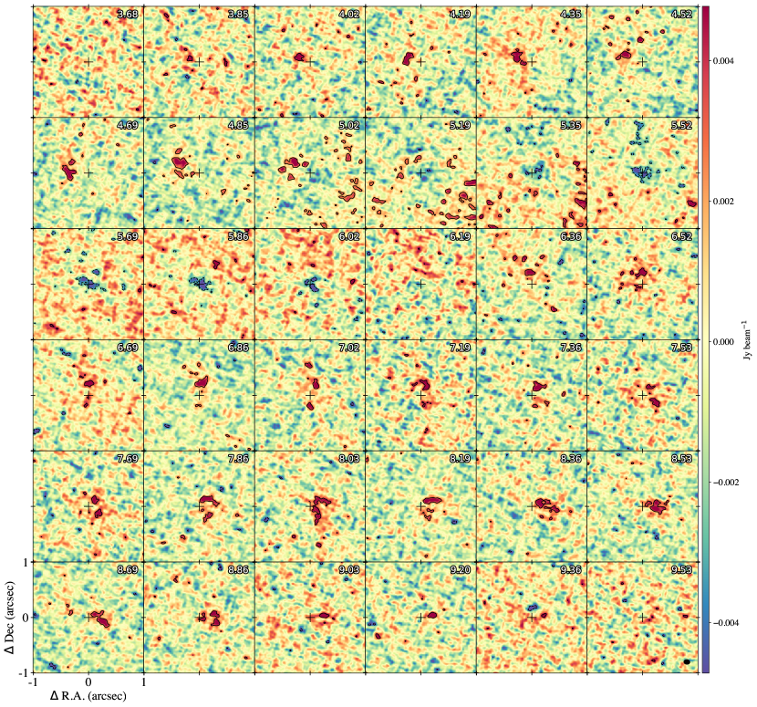
Figure 19: Channel maps showing the zoomed-in view of the C¹⁸O (2–1) emission around IRS5N. The numbers at the top show the corresponding velocity of each channel map. The solid contours represent the 3$\sigma$ level and the dashed lines show the $-3\sigma$ level. The cross shows the peak position of the IRS5N continuum. Synthesized beam is shown in black on the bottom right corner of the final channel.

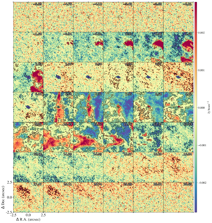
Figure 20: Same as Figure 19 but for ¹²CO (2–1) instead.

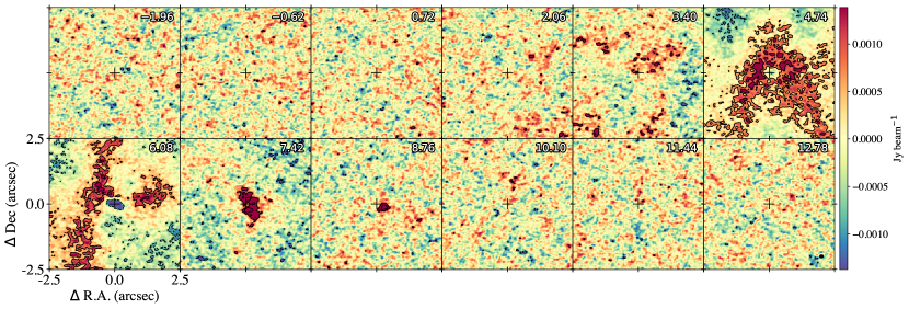
Figure 22: Same as Figure 19 but for H₂CO (3_0,3–2_0,2) instead.

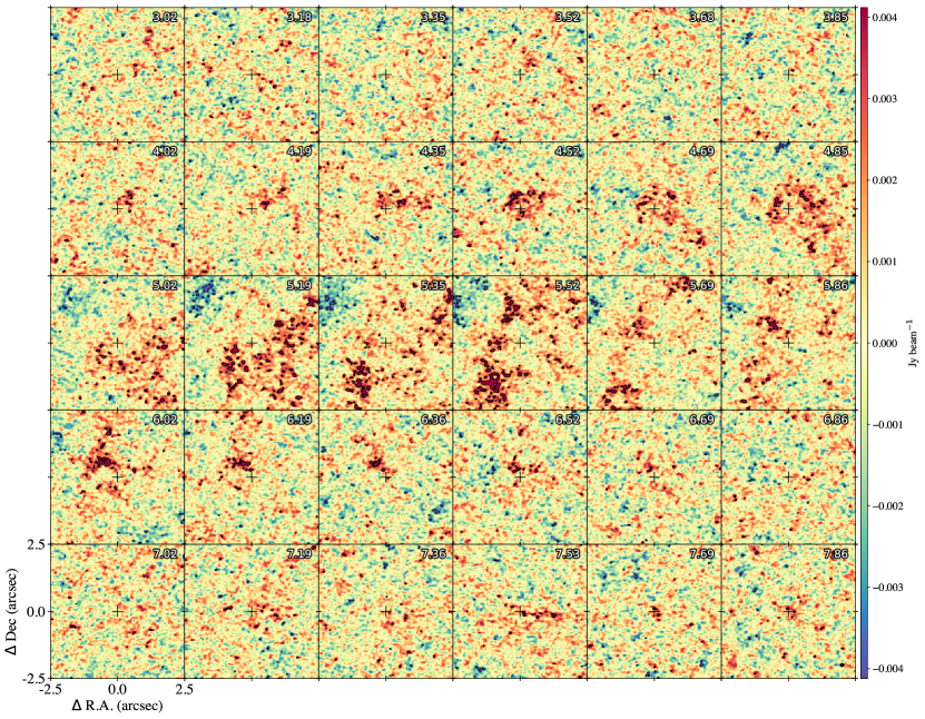
Figure 23: Same as Figure 19 but for H₂CO (3_2,1–2_2,0) instead.

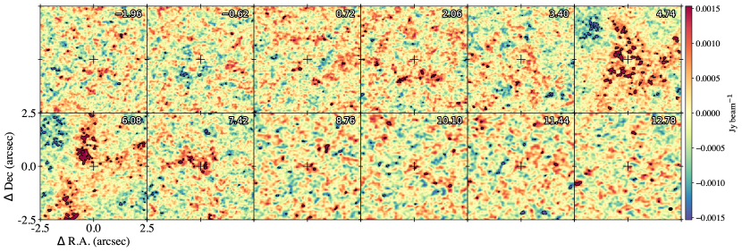
Figure 24: Same as Figure 19 but for H₂CO (3_2,2–2_2,1) instead.

References

- ALMA Partnership et al. (2015) ALMA Partnership, Brogan, C. L., Pérez, L. M., et al. 2015, ApJ, 808, L3, doi: 10.1088/2041-8205/808/1/L3
- Andrews & Williams (2005) Andrews, S. M., & Williams, J. P. 2005, ApJ, 631, 1134, doi: 10.1086/432712
- Andrews et al. (2018) Andrews, S. M., Huang, J., Pérez, L. M., et al. 2018, The Astrophysical Journal Letters, 869, L41, doi: 10.3847/2041-8213/aaf741
- Ansdell et al. (2016) Ansdell, M., Williams, J. P., van der Marel, N., et al. 2016, ApJ, 828, 46, doi: 10.3847/0004-637X/828/1/46
- Aso & Sai (2023) Aso, Y., & Sai, J. 2023, jinshisai/SLAM: First Release of SLAM, v1.0.0, Zenodo, doi: 10.5281/zenodo.7783868
- Astropy Collaboration et al. (2018) Astropy Collaboration, Price-Whelan, A. M., Sipőcz, B. M., et al. 2018, AJ, 156, 123, doi: 10.3847/1538-3881/aabc4f
- Beckwith et al. (1990) Beckwith, S. V. W., Sargent, A. I., Chini, R. S., & Guesten, R. 1990, AJ, 99, 924, doi: 10.1086/115385
- Benisty et al. (2021) Benisty, M., Bae, J., Facchini, S., et al. 2021, ApJ, 916, L2, doi: 10.3847/2041-8213/ac0f83
- Brinch & Jørgensen (2013) Brinch, C., & Jørgensen, J. K. 2013, A&A, 559, A82, doi: 10.1051/0004-6361/201322463
- Busch et al. (2020) Busch, L. A., Belloche, A., Cabrit, S., Hennebelle, P., & Commerçon, B. 2020, A&A, 633, A126, doi: 10.1051/0004-6361/201936432
- Chen & Graham (1993) Chen, W. P., & Graham, J. A. 1993, ApJ, 409, 319, doi: 10.1086/172665
- Chiang & Goldreich (1997) Chiang, E. I., & Goldreich, P. 1997, ApJ, 490, 368, doi: 10.1086/304869
- Chini et al. (2003) Chini, R., Kämpgen, K., Reipurth, B., et al. 2003, A&A, 409, 235, doi: 10.1051/0004-6361:20031115
- Cieza et al. (2021) Cieza, L. A., González-Ruilova, C., Hales, A. S., et al. 2021, MNRAS, 501, 2934, doi: 10.1093/mnras/staa3787
- Commerçon et al. (2012) Commerçon, B., Launhardt, R., Dullemond, C., & Henning, T. 2012, A&A, 545, A98, doi: 10.1051/0004-6361/201118706
- Dong et al. (2015) Dong, R., Zhu, Z., & Whitney, B. 2015, ApJ, 809, 93, doi: 10.1088/0004-637X/809/1/93
- Dutta et al. (2022) Dutta, S., Lee, C.-F., Hirano, N., et al. 2022, ApJ, 931, 130, doi: 10.3847/1538-4357/ac67a1
- Galli et al. (2020) Galli, P. A. B., Bouy, H., Olivares, J., et al. 2020, A&A, 643, A148, doi: 10.1051/0004-6361/202038717
- Gonzalez et al. (2017) Gonzalez, J. F., Laibe, G., & Maddison, S. T. 2017, MNRAS, 467, 1984, doi: 10.1093/mnras/stx016
- Harju et al. (1993) Harju, J., Haikala, L. K., Mattila, K., et al. 1993, A&A, 278, 569
- Harris et al. (2020) Harris, C. R., Millman, K. J., van der Walt, S. J., et al. 2020, Nature, 585, 357, doi: 10.1038/s41586-020-2649-2
- Huang et al. (2018) Huang, J., Andrews, S. M., Dullemond, C. P., et al. 2018, ApJ, 869, L42, doi: 10.3847/2041-8213/aaf740
- Hunter (2007) Hunter, J. D. 2007, Computing in Science & Engineering, 9, 90, doi: 10.1109/MCSE.2007.55
- Isella et al. (2019) Isella, A., Benisty, M., Teague, R., et al. 2019, ApJ, 879, L25, doi: 10.3847/2041-8213/ab2a12
- Jørgensen et al. (2022) Jørgensen, J. K., Kuruwita, R. L., Harsono, D., et al. 2022, Nature, 606, 272, doi: 10.1038/s41586-022-04659-4
- Jørgensen et al. (2002) Jørgensen, J. K., Schöier, F. L., & van Dishoeck, E. F. 2002, A&A, 389, 908, doi: 10.1051/0004-6361:20020681
- Jørgensen et al. (2015) Jørgensen, J. K., Visser, R., Williams, J. P., & Bergin, E. A. 2015, A&A, 579, A23, doi: 10.1051/0004-6361/201425317
- Keppler et al. (2018) Keppler, M., Benisty, M., Müller, A., et al. 2018, A&A, 617, A44, doi: 10.1051/0004-6361/201832957
- Kratter & Lodato (2016) Kratter, K., & Lodato, G. 2016, ARA&A, 54, 271, doi: 10.1146/annurev-astro-081915-023307
- Kristensen et al. (2012) Kristensen, L. E., van Dishoeck, E. F., Bergin, E. A., et al. 2012, A&A, 542, A8, doi: 10.1051/0004-6361/201118146
- Kuffmeier et al. (2019) Kuffmeier, M., Calcutt, H., & Kristensen, L. E. 2019, A&A, 628, A112, doi: 10.1051/0004-6361/201935504
- Kusaka et al. (1970) Kusaka, T., Nakano, T., & Hayashi, C. 1970, Progress of Theoretical Physics, 44, 1580, doi: 10.1143/PTP.44.1580
- Lindberg et al. (2014) Lindberg, J. E., Jørgensen, J. K., Green, J. D., et al. 2014, A&A, 565, A29, doi: 10.1051/0004-6361/201322184
- Maret et al. (2020) Maret, S., Maury, A. J., Belloche, A., et al. 2020, A&A, 635, A15, doi: 10.1051/0004-6361/201936798
- Maureira et al. (2020) Maureira, M. J., Arce, H. G., Dunham, M. M., et al. 2020, MNRAS, 499, 4394, doi: 10.1093/mnras/staa2894
- McKee & Ostriker (2007) McKee, C. F., & Ostriker, E. C. 2007, ARA&A, 45, 565, doi: 10.1146/annurev.astro.45.051806.110602
- McMullin et al. (2007) McMullin, J. P., Waters, B., Schiebel, D., Young, W., & Golap, K. 2007, in Astronomical Society of the Pacific Conference Series, Vol. 376, Astronomical Data Analysis Software and Systems XVI, ed. R. A. Shaw, F. Hill, & D. J. Bell, 127
- Neuhäuser & Forbrich (2008) Neuhäuser, R., & Forbrich, J. 2008, in Handbook of Star Forming Regions, Volume II, ed. B. Reipurth, Vol. 5, 735
- Nisini et al. (2005) Nisini, B., Antoniucci, S., Giannini, T., & Lorenzetti, D. 2005, A&A, 429, 543, doi: 10.1051/0004-6361:20041409
- Nutter et al. (2005) Nutter, D. J., Ward-Thompson, D., & André, P. 2005, MNRAS, 357, 975, doi: 10.1111/j.1365-2966.2005.08711.x
- Ohashi et al. (2014) Ohashi, N., Saigo, K., Aso, Y., et al. 2014, ApJ, 796, 131, doi: 10.1088/0004-637X/796/2/131
- Ohashi et al. (2023) Ohashi, N., Tobin, J. J., Jørgensen, J. K., et al. 2023, ApJ, 951, 8, doi: 10.3847/1538-4357/acd384
- Peterson et al. (2011) Peterson, D. E., Caratti o Garatti, A., Bourke, T. L., et al. 2011, ApJS, 194, 43, doi: 10.1088/0067-0049/194/2/43
- Robitaille (2019) Robitaille, T. 2019, APLpy v2.0: The Astronomical Plotting Library in Python, doi: 10.5281/zenodo.2567476
- Robitaille & Bressert (2012) Robitaille, T., & Bressert, E. 2012, APLpy: Astronomical Plotting Library in Python, Astrophysics Source Code Library. http://ascl.net/1208.017
- Sadavoy et al. (2018) Sadavoy, S. I., Myers, P. C., Stephens, I. W., et al. 2018, ApJ, 869, 115, doi: 10.3847/1538-4357/aaef81
- Sakai et al. (2014) Sakai, N., Sakai, T., Hirota, T., et al. 2014, Nature, 507, 78, doi: 10.1038/nature13000
- Sandell et al. (2021) Sandell, G., Reipurth, B., Vacca, W. D., & Bajaj, N. S. 2021, ApJ, 920, 7, doi: 10.3847/1538-4357/ac133d
- Schilke et al. (1997) Schilke, P., Walmsley, C. M., Pineau des Forets, G., & Flower, D. R. 1997, A&A, 321, 293
- Segura-Cox et al. (2020) Segura-Cox, D. M., Schmiedeke, A., Pineda, J. E., et al. 2020, Nature, 586, 228, doi: 10.1038/s41586-020-2779-6
- Sharma et al. (2020) Sharma, R., Tobin, J. J., Sheehan, P. D., et al. 2020, ApJ, 904, 78, doi: 10.3847/1538-4357/abbdf4
- Sheehan & Eisner (2017) Sheehan, P. D., & Eisner, J. A. 2017, ApJ, 851, 45, doi: 10.3847/1538-4357/aa9990
- Sheehan et al. (2020) Sheehan, P. D., Tobin, J. J., Federman, S., Megeath, S. T., & Looney, L. W. 2020, ApJ, 902, 141, doi: 10.3847/1538-4357/abbad5
- Simon et al. (2000) Simon, M., Dutrey, A., & Guilloteau, S. 2000, ApJ, 545, 1034, doi: 10.1086/317838
- Takakuwa et al. (in prep.) Takakuwa, S., Ohashi, N., Jørgensen, J. K., Tobin, J. J., & eDisk Team. in prep., ApJ
- Taylor & Storey (1984) Taylor, K. N. R., & Storey, J. W. V. 1984, MNRAS, 209, 5P, doi: 10.1093/mnras/209.1.5P
- Terebey et al. (1984) Terebey, S., Shu, F. H., & Cassen, P. 1984, ApJ, 286, 529, doi: 10.1086/162628
- Testi et al. (2014) Testi, L., Birnstiel, T., Ricci, L., et al. 2014, in Protostars and Planets VI, ed. H. Beuther, R. S. Klessen, C. P. Dullemond, & T. Henning, 339, doi: 10.2458/azu_uapress_9780816531240-ch015
- Tobin et al. (2012) Tobin, J. J., Hartmann, L., Chiang, H.-F., et al. 2012, Nature, 492, 83, doi: 10.1038/nature11610
- Tobin et al. (2016) Tobin, J. J., Kratter, K. M., Persson, M. V., et al. 2016, Nature, 538, 483, doi: 10.1038/nature20094
- Tobin et al. (2020) Tobin, J. J., Sheehan, P. D., Megeath, S. T., et al. 2020, ApJ, 890, 130, doi: 10.3847/1538-4357/ab6f64
- Tomida et al. (2015) Tomida, K., Okuzumi, S., & Machida, M. N. 2015, ApJ, 801, 117, doi: 10.1088/0004-637X/801/2/117
- Tychoniec et al. (2020) Tychoniec, Ł., Manara, C. F., Rosotti, G. P., et al. 2020, A&A, 640, A19, doi: 10.1051/0004-6361/202037851
- van der Wiel et al. (2019) van der Wiel, M. H. D., Jacobsen, S. K., Jørgensen, J. K., et al. 2019, A&A, 626, A93, doi: 10.1051/0004-6361/201833695
- Wakelam et al. (2005) Wakelam, V., Ceccarelli, C., Castets, A., et al. 2005, A&A, 437, 149, doi: 10.1051/0004-6361:20042566
- Wang et al. (2004) Wang, H., Mundt, R., Henning, T., & Apai, D. 2004, ApJ, 617, 1191, doi: 10.1086/425493
- Zhang et al. (2015) Zhang, K., Blake, G. A., & Bergin, E. A. 2015, The Astrophysical Journal Letters, 806, L7, doi: 10.1088/2041-8205/806/1/L7
- Zhang et al. (2018) Zhang, S., Zhu, Z., Huang, J., et al. 2018, The Astrophysical Journal Letters, 869, L47, doi: 10.3847/2041-8213/aaf744
- Zucker et al. (2020) Zucker, C., Speagle, Joshua S., Schlafly, Edward F., et al. 2020, A&A, 633, A51, doi: 10.1051/0004-6361/201936145