f-mode oscillations of anisotropic neutron stars in full general relativity

Abstract

We investigate f-mode oscillations of anisotropic, non-rotating, neutron stars within the framework of full general relativity (up to the linear order perturbation), considering both the metric and the fluid perturbations. We first present the equations governing unperturbed stellar structures as well as oscillations under a phenomenological ansatz to account for the local anisotropy. Then, we solve those equations for two different equations of states, namely BSk21 and BSk19, the former being stiffer than the latter. For both of the cases, we consider only stable neutron stars. We see that, moderately anisotropic neutron stars with the tangential pressure larger than the radial pressure can give more massive neutron stars than the isotropic or very anisotropic ones. We find that the frequency of the f-mode exhibits a linear relationship with the square root of the average density of neutron stars and the slope of the linear fit depends on the anisotropic strength. We also see that, for any given value of the anisotropic strength, neutron stars of higher masses have higher values of the frequency. For lower values of the mass, the increase of the frequency with the mass is linear, but for higher values of the mass, the frequency increases rapidly with the increase in the value of the mass. However, this non-linear rise in the frequency with the mass is not prominent when the radial pressure is larger than the tangential pressure. We also see that for a fixed value of a small mass, higher anisotropy leads to a larger value of the frequency, but when the fixed mass is above a threshold value, higher anisotropy leads to a smaller value of the frequency. Moreover, for a fixed mass of the neutron star and for the same amount of the anisotropy, the value of the frequency is higher for the softer equation of state, but the nature of the variation in the frequency with the change in the anisotropic strength is similar for the two equations of state. We also find that the damping time of the f-mode oscillation decreases as the mass of the neutron star increases for all values of the anisotropic strength. However, for mildly anisotropic neutron stars, a slight increase in the damping time occurs near the stable maximum mass. Moreover, for a fixed mass of the neutron star and for the same amount of the anisotropy, the value of the damping time is lower for the softer equation of state, but the nature of the variation in the damping time with the change in the anisotropic strength is similar for the two equations of state.

I Introduction

Among various heavenly bodies throughout the universe, neutron stars are one of the exotic objects, mainly because of their extremely high densities. Hence, general relativity plays a very important role to describe the overall structure of a neutron star. Neutron stars and less denser white dwarfs form the compact star family.

To model the structure of neutron stars and associated properties, usually it is assumed that the pressure inside the neutron star is isotropic. However, one can not rule out the possibility of anisotropy in the pressure inside a neutron star. The idea of the tangential pressure being different than the radial pressure can be traced long back to Lemaitre [1]. Bowers and Liang [2] was the first to apply the anisotropic model on the equilibrium configuration of relativistic compact stars. They showed that the local anisotropy in compact stars have non negligible effects on the observable properties like the mass, the surface redshift, etc. It is claimed that, at the high density regime ($10^{14}-10^{15}{\rm~{}g\,cm^{-3}}$), where the inter particle interactions become relativistic, anisotropy should be present in the system [3]. The pressure anisotropy can be triggered by various phenomena, e.g., the presence of a solid core [4, 5], superfluidity [6], pion condensation [7], slow rotation [8], the mixture of two fluids [9], etc. The presence of the viscosity can also induce local anisotropy inside the compact stars [10, 11]. Yazadjiev [12] modeled magnetars in general relativity in a nonperturbative way, where the constituent fluid was considered anisotropic due to the presence of the magnetic field. Recently, Deb et al. [13] showed that the magnetic field introduces an additional anisotropy, and alters various properties like the mass, the radius, the surface redshift, etc., of compact stars. Elasticity in compact stars can also be described by the local anisotropy [14]. Additional studies related to anisotropic pressure inside neutron stars have been described in Herrera and Santos [15] and the references therein.

Neutron stars are laboratories to study various theories of physics at high densities. These objects are observed in a wide range of the electromagnetic spectrum, but there are various properties that can not be probed through electromagnetic waves. The recent detections of gravitational waves have opened up a completely new window for the observation of neutron stars and other compact objects. So far, only the gravitational waves emitted during the late inspiral, merger and ringdown phase of the components of binary systems of compact objects have been detected by ground based detectors [16, 17, 18]. Recently, Pulsar Timing Array collaboration has found the evidence of gravitational waves in the nanohertz regime [19, 20, 21]. In the future, it is expected that detectors like LISA (Laser Interferometer Space Antenna), Einstein telescope, etc., would detect gravitational waves generated from various sources and help us look deep into the cosmos and give us idea of many other objects. The oscillations of neutron stars is one of the promising sources of gravitational waves. At the last phase of the life cycle of a massive star, a supernova explosion occurs, and the newly formed neutron star might oscillate violently. Other than that, if the merger of two compact stars form a neutron star, then that object would also oscillates. A part of the energy of the oscillation, would be emitted as the gravitational radiation, which would propagate as ripples of space-time or gravitational waves. Due to the emission of the gravitational waves, the oscillation would get damped. Thorne and Campolattaro [22] first theoretically studied the non-radial oscillations of neutron stars within the framework of full general relativity. Later, Lindblom and Detweiler [23], Detweiler and Lindblom [24] did the similar calculations with some modifications. Using the same formalism, the non-radial oscillation modes are calculated for superfluid neutron stars [25], quark stars [26], neutron stars with density discontinuity [27, 28], etc. Recent studies on the impact of the equation of state on the neutron star oscillation modes reveal the fact that the nuclear interaction has important effects on the quasi-normal modes [29]. Most of these studies assume pressure isotropy inside the neutron stars. The effects of anisotropy on non-radial oscillation modes were first studied by Hillebrandt and Steinmetz [30] in the Newtonian frame work. This study revealed the fact that the pressure anisotropy plays a very important role on the mode frequencies. Later, Doneva and Yazadjiev [31] calculated f-mode and p-mode frequencies in the Cowling approximation, where they have ignored the metric perturbation. In a recent study, Curi et al. [32] extended this work for the case of realistic equation of states. All of the above mentioned studies showed that the anisotropy in neutron stars can change the numerical value of the frequencies of the quasi-normal modes. Although the metric perturbation is ignored, Cowling approximation gives accurate enough results for fluid perturbations. However, the possibilities of errors due to ignoring the metric perturbation might not be negligible. Recently, Sotani and Takiwaki [33] found that the mode frequencies under Cowling approximation are estimated within $~{}20\%$ accuracy. Another draw back in Cowling approximation is the fact that, as the metric perturbation is ignored, the energy loss due to the gravitational waves is also unaccounted for. In the full framework of general relativity taking into account of perturbations of the metric, the oscillation of the metric propagates as gravitational waves, which carry away the energy of the oscillations. As a result, the oscillation experiences damping, leading to a decrease in its amplitude over time. The characteristic time associated with this damping is known as the damping time and has been mathematically defined at the end of Sec. III.2. The damping time can not be calculated by Cowling approximation.

The motivation of the present work is to study the quasi-normal modes of anisotropic neutron stars within the framework of full general relativity. Our focus is mainly to derive the governing differential equations for f-mode oscillation of neutron stars with pressure anisotropy, and to find the mode frequencies and the damping times. Moreover, we study only polar perturbations, characterized by the metric perturbation functions that exhibit even parity under the spatial inversion ($(\theta,\phi)\rightarrow(\pi-\theta,\pi+\phi)$), where $r$, $\theta$, and $\phi$ denote coordinates within a spherical polar coordinate system. Out of the various polar modes, we focus on the fundamental (f) modes. We have considered mainly BSk21 equation of state, which connects the radial pressure with the density inside the neutron stars. To describe the tangential pressure, we have considered a phenomenological ansatz described by Horvat et al. [34]. We show how the f-mode frequency and the associated damping time change due to the presence of the pressure anisotropy, for various masses of neutron stars, as well as various extent of the anisotropy inside those.

The paper is organized as follows. In Sec. II, we detail the equilibrium model of anisotropic neutron stars. This involves presenting the modified Tolman-Oppenheimer-Volkoff (TOV) equations due to anisotropy, describing the equation of state (EoS), and outlining the anisotropy ansatz. Moving to Sec. III, we delve into the perturbation scheme for neutron stars. This section covers both of the analytical and numerical techniques employed to compute the frequencies and the damping times of f-mode oscillations. In Sec. IV, we present our results. Finally, we conclude the paper in Sec. V with a summary and discussion of our findings. In this paper, all mathematical expressions are written in the natural units, setting $G=1$, $c=1$, where $G$ is the gravitational constant and $c$ is the speed of light in vacuum.

II Equilibrium configuration of anisotropic neutron stars in general relativity

In case of a spherically symmetric non-rotating space-time, the metric can be written in the well known form

$$ds^{2}=-e^{\nu(r)}dt^{2}+e^{\lambda(r)}dr^{2}+r^{2}(d\theta^{2}+\sin^{2}\theta d\phi^{2}),$$ (1)

where $\nu(r)$ and $\lambda(r)$ are metric functions that depend on the radial coordinate ($r$) only. We take an anisotropic fluid as the matter source in the field equations, where the radial component of the pressure $(p_{r})$ and the tangential component of the pressure $(p_{t})$ are non-identical. Note that, like the metric functions, the radial and the tangential components of the pressure inside a neutron star also depend on $r$. However, for the sake of simplicity, from now on, we will not write the $r$ dependence explicitly.

The anisotropy parameter is defined as,

$$\chi=p_{t}-p_{r}.$$ (2)

Note that, in this article, the anisotropy parameter $\chi$ is described similar to the anisotropy parameter by Horvat et al. [34], whereas some other studies [31, 32] describe the anisotropy parameter as $(p_{r}-p_{t})$. The energy momentum tensor of the anisotropic fluid can be written in the form [35, 36]

$$T_{~{}\alpha}^{\beta}=(\rho+p_{t})u^{\beta}u_{\alpha}+\delta_{~{}\alpha}^{\beta}\,p_{t}+(p_{r}-p_{t})s^{\beta}s_{\alpha},$$ (3)

where $\rho$ is the fluid matter density. The space-like radial unit vector $s^{\alpha}$ is defined as:

$$s^{\alpha}=(0,e^{-\lambda/2},0,0),$$ (4)

and the fluid 4-velocity vector is given by:

$$u^{\beta}=(e^{-\nu/2},0,0,0),$$ (5)

which satisfy the conditions

$$u^{\alpha}u_{\alpha} =-1,$$ (6a)

$$s^{\alpha}s_{\alpha} =1,$$ (6b)

$$s^{\beta}u_{\beta} =0.$$ (6c)

The non zero components of the energy momentum tensor ($T_{~{}\alpha}^{\beta}$) are only $diag(-\rho,p_{r},p_{t},p_{t})$. The space-time geometry and the matter distribution are related by Einstein equations

$$G_{~{}\alpha}^{\beta}=8\pi T_{~{}\alpha}^{\beta},$$ (7)

where $G_{~{}\alpha}^{\beta}$ is the Einstein tensor, describing the spacetime geometry. Using equations (1) and (3), the Einstein equations can be written as:

$$e^{-\lambda}\left(\frac{\lambda^{\prime}}{r}-\frac{1}{r^{2}}\right)+\frac{1}{r^{2}}=8\pi\rho,$$ (8)

$$e^{-\lambda}\left(\frac{\nu^{\prime}}{r}+\frac{1}{r^{2}}\right)-\frac{1}{r^{2}}=8\pi p_{r},$$ (9)

$$\frac{1}{2}e^{-\lambda}\left(\nu^{\prime\prime}-\frac{1}{2}\nu^{\prime}\lambda^{\prime}+\frac{1}{2}{\nu^{\prime}}^{2}+\frac{\nu^{\prime}-\lambda^{\prime}}{r}\right)=8\pi p_{t},$$ (10)

where a prime denotes the differentiation with respect to $r$. From equations (8), (9), and (10), we get the equation of hydrostatic equilibrium in the presence of the pressure anisotropy, which can be written as (in natural units):

$$p_{r}^{\prime}=-\frac{\nu^{\prime}}{2}(\rho+p_{r})+\frac{2\chi}{r}.$$ (11)

The interior metric function ($r<R$, where $R$ is the radius of the star) can be found from Eq. (8) as:

$$e^{-\lambda}=1-\frac{2m}{r},\text{ where }m=4\pi\int_{0}^{r}\rho(r^{\prime})r^{\prime 2}dr^{\prime}~{},$$ (12)

is the mass enclosed within a spherical region of radius $r$ inside the star. Using Eqs. (9) and (12), the hydrostatic equilibrium equation (11) can be written as:

$$p_{r}^{\prime}=-\frac{(\rho+p_{r})(m+4\pi p_{r}r^{3})}{r(r-2m)}+\frac{2\chi}{r}.$$ (13)

This is the modified Tolman-Oppenheimer-Volkoff (TOV) equation, which takes the local pressure anisotropy into account. To solve this equation, we need to specify the equation of state of the neutron star matter, i.e., the dependence of $p_{r}$ on $\rho$ and the anisotropy parameter $\chi$. As the boundary conditions, we set a finite radial pressure at the center of the star and zero radial pressure at the surface of the star. This also implies zero density at the surface of the star.

Other than these conditions, the metric functions should match with the exterior Schwarzschild metric at $r=R$, i.e.,

$$\lambda(R)=-\nu(R)=-\ln\left(1-\frac{2M}{R}\right),$$ (14)

where $M$ is the total mass of the star, i.e., $M=m(R)$.

II.1 Description of the equation of state and the anisotropy parameter

As mentioned earlier, to build a model of neutron stars, i.e., to solve the modified TOV equation (Eq.(13)), one needs to specify how the pressure inside the stars varies with the density, which is known as the equation of state (EoS). There are studies of microscopic physics leading to various Equations of State (EsoS)[37, 38, and references therein].

However, those studies are usually for isotropic matter, and no rigorous study has been performed to model the pressure anisotropy inside a neutron star. Hence, people use different ansatzes for the anisotropy parameter $\chi$. One popular ansatz for $\chi$ was proposed by Horvat et al. [34] as:

$$\chi=\tau p_{r}\mu,$$ (15)

where $\mu=2m/r$ is the local compactness and $\tau$ is a parameter governing the strength of the anisotropy. Consistent with previous studies [31, 39, 40], we consider values of $\tau$ within the range $-2\leq\tau\leq 2$. The chosen form of the anisotropy parameter in Eq. (15) possesses two appealing characteristics. First, the anisotropy parameter vanishes at the center of the star, as the compactness scales as $\mu\sim r^{2}$ when $r\to 0$, ensuring the regularity of the anisotropy parameter. Second, in the non-relativistic regime, where $\mu$ is significantly smaller than unity, the impact of the pressure anisotropy is expected to be negligible. The chosen ansatz satisfies this.

In the present work, we use the above ansatz for the anisotropy in association with the analytical representation of the Brussels - Montreal unified EoS for the nuclear matter, referred to as BSk19, BSk20, BSk21 [41, 42, 43], which model $p_{r}(\rho)$ with two parameters $\zeta$ and $\sigma$ that are parametrised as [44]:

$$\begin{split}\zeta=\frac{a_{1}+a_{2}\sigma+a_{3}\sigma^{3}}{1+a_{4}\sigma}f(a_{5}(\sigma-a_{6}))&+(a_{7}+a_{8}\sigma)f(a_{9}(a_{6}-\sigma))+(a_{10}+a_{11}\sigma)f(a_{12}(a_{13}-\sigma))\\ &+(a_{14}+a_{15}\sigma)f(a_{16}(a_{17}-\sigma))+\frac{a_{18}}{1+[a_{19}(\sigma-a_{20})]^{2}}+\frac{a_{21}}{1+[a_{22}(\sigma-a_{23})]^{2}},\end{split}$$ (16)

where $\zeta=\log_{10}(p_{r}\,{\rm~{}in~{}dyn~{}cm^{-2}})$, $\sigma=\log_{10}(\rho\,{\rm~{}in~{}g~{}cm^{-3}})$, and $f(x)=[\exp(x)+1]^{-1}$. The values of the coefficients $a_{i}(i=1,\ldots,23)$ can be found in Potekhin et al. [44]. Throughout this article, our analysis primarily uses BSk21 EoS. However, to compare our results across different levels of matter stiffness, we also consider the BSk19 EoS in selected cases.

Although one can solve the modified TOV equation for various values of the central density ($\rho_{c}$) and the anisotropic strength, but all of the resulting neutron stars would not be stable. First, to avoid the spontaneous collapse of the matter, the pressure should be monotonically nondecreasing function of the density [45], i.e., $\partial p_{r}/\partial\rho>0$ and $\partial p_{t}/\partial\rho>0$. Second, the speed of sound can not be negative, i.e., $v_{sr}>0$ and $v_{st}>0$, where $v_{sr}$ and $v_{st}$ are the speed of sound in the radial and the tangential directions, respectively, defined by $v_{sr}^{2}=\partial p_{r}/\partial\rho$ and $v_{st}^{2}=\partial p_{t}/\partial\rho$. Any realistic EoS satisfy the condition $v_{sr}>0$. However, as we do not have very rigorous studies on the pressure anisotropy, we rather use some plausible ansatzes, for a chosen set of EoS and anisotropy ansatz, the condition $v_{st}>0$ might be violated for some (or all) values of the density and hence should be checked. Third, the causality condition should be satisfied, i.e., $v_{sr}<v_{\rm light}$ and $v_{st}<v_{\rm light}$, where $v_{\rm light}$ is the speed of light in the neutron star matter. As we do not know the value of $v_{\rm light}$, we set it as $v_{\rm light}=0.95\,c$ where $c$ is the speed of light in vacuum (1 in the natural unit). Fourth, the neutron star must be stable under radial oscillation, which is possible only when $\partial M/\partial\rho_{c}>0$ [46].

To check the validity of our chosen EsoS, the anisotropy ansatz, and the range of the anisotropic strength $\tau$, in Figs. 1 and 2, we plot the values of the total mass obtained by solving the modified TOV equation against the corresponding values of the central densities for various values of $\tau$ for BSk21 and BSk19 EsoS respectively. In both of these figures, filled circles on each profile represent the points where $\partial M/\partial\rho_{c}=0$, the six pointed stars present the values of $\rho_{c}$ up to which $v_{sr}\leq 0.95$ throughout the star, the filled squares present the values of $\rho_{c}$ up to which $v_{st}\leq 0.95$ throughout the star, and the filled triangles denote the values of $\rho_{c}$ up to which $v_{st}\geq 0$ throughout the star.

We see that, for both BSk21 and BSk19 EsoS, as the value of $\tau$ increases, the maximum value of the central density up to which we get neutron stars that are stable against radial oscillations decreases. Moreover, for $\tau\leq 0$, $v_{sr}$ reach the value $0.95$ inside neutron stars with the value of the central density smaller than the value of the central density of neutron stars for which $\partial M/\partial\rho_{c}=0$, and $v_{st}$ reach the limit of $0.95$ even before that. The situation is the opposite when $\tau=0$. For sufficiently large values of $\tau$, e.g., 1.5 and higher, $v_{st}$ never reaches the causal limit $0.95$. However, for such values of $\tau$, the value of $v_{st}$ does not remain positive throughout the star, except for very small values of $\rho_{c}$. On the other hand, for the chosen set of EsoS, the anisotropy ansatz, and the range of the values of $\tau$, $v_{sr}$ always remains positive throughout the star.

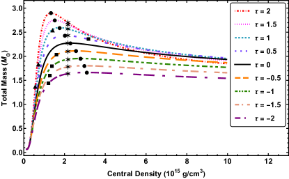
Figure 1: Mass-Central density profiles for anisotropic neutron stars with $-2\leq\tau\leq 2$ for BSk21 EoS. Filled circles on each profile represent the points where $\partial M/\partial\rho_{c}=0$, the six pointed stars present the values of $\rho_{c}$ up to which $v_{sr}\leq 0.95$ throughout the star, the filled squares present the values of $\rho_{c}$ up to which $v_{st}\leq 0.95$ throughout the star, and the filled triangles denote the values of $\rho_{c}$ up to which $v_{st}\geq 0$ throughout the star.

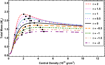
Figure 2: Mass-Central density profiles for anisotropic neutron stars with $-2\leq\tau\leq 2$ for BSk19 EoS. Filled circles on each profile represent the points where $\partial M/\partial\rho_{c}=0$, the six pointed stars present the values of $\rho_{c}$ up to which $v_{sr}\leq 0.95$ throughout the star, the filled squares present the values of $\rho_{c}$ up to which $v_{st}\leq 0.95$ throughout the star, and the filled triangles denote the values of $\rho_{c}$ up to which $v_{st}\geq 0$ throughout the star.

Next, we plot the mass$-$radius curves for various values of $\tau$ (in the range of $-2$ to 2, as mentioned earlier) for BSk21 EoS in Fig. 3 and for BSk19 EoS in Fig. 4, both only up to the masses that satisfy all of the four stability conditions discussed earlier. In both of the figures, in addition to mass-radius curves, we have shown the measured mass ranges of PSR J2045$+$3633 [47] and PSR J0952$-$0607 [48], representing a low-mass ($\rm 1.252\pm 0.021~{}M_{\odot}$) and a high mass ($\rm 2.35\pm 0.17~{}M_{\odot}$) neutron star, respectively, as well as the band for the event GW190814 [49], corresponding to an object after merger in the mass range of $\rm 2.50-2.67~{}M_{\odot}$. This object lies in the so-called “mass gap”, implying that it could be either a highly massive neutron star or a light black hole.

We see that for a range of the anisotropic strength, BSk21 EoS can lead to neutron stars massive enough to satisfy all three measurements. However, BSk19 EoS fails to produce masses higher than $2.1~{}{\rm M_{\odot}}$. Hence, we prefer BSk21 EoS, although we can not rule out a softer EoS like BSk19 EoS. Especially, if we keep in mind the fact that it might be possible to get such massive neutron stars in some other ansatz for the anisotropy even for BSk19 EoS.

Note that, all our calculations, i.e., obtaining the stellar structure by solving the modified TOV equation (as presented in this section) and the study of f-mode oscillations (will be presented in the next two sections), are done within the static limit, i.e., for non-rotating stars. Hence, we do not show the excluded region known as the ‘mass-shedding limit’ for low mass neutron stars where the rotating neutron stars break due to the centrifugal force. However, observed neutron stars are known to be fast rotators. In particular, the spin frequencies of PSR J2045$+$3633 and PSR J0952$-$0607 are 31.56 Hz [47] and 707.31 Hz [50], respectively. Hence, low mass neutron stars ($\lesssim 0.5~{}{\rm M_{\odot}}$) can not exist in the nature, although we show them in Figs. 3, 4.

The use of the static configuration does not affect the stellar structure significantly for the neutron stars of high masses. As an example, Bagchi [51] showed that the maximum mass for a stable, non-rotating isotropic neutron star with APR EoS is 2.19 ${\rm M_{\odot}}$ whereas the maximum mass for a stable isotropic neutron stars rotating with a spin frequency of 796 Hz (with APR EoS) is 2.20 ${\rm M_{\odot}}$. This can justify our choice of studying even anisotropic neutron stars in the static limit. It will be interesting to study in the future both the stellar structure and f-mode oscillations of anisotropic neutron stars under full general relativistic framework including the rotation.

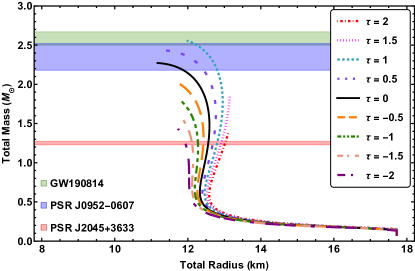
Figure 3: Mass-Radius profiles for anisotropic stable neutron stars with $-2\leq\tau\leq 2$ and BSk21 EoS.

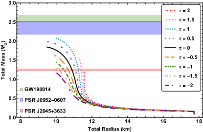
Figure 4: Mass-Radius profiles for anisotropic neutron stars with $-2\leq\tau\leq 2$ and BSk19 EoS.

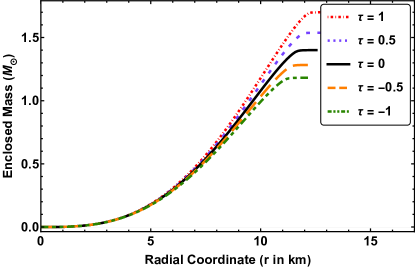
Figure 5: Variation of the enclosed mass with the radial coordinate inside neutron stars for various values of the anisotropic strength, each for $\rho_{c}=~{}7.2955\times 10^{14}~{}{\rm g\,cm^{-3}}$ and BSk21 EoS.

Figure 5, we plot the radial coordinate (in km) inside the neutron star along the abscissa, and the corresponding enclosed mass in the unit of solar mass along the ordinate for BSk21 EoS. Various curves in this figure represent different values of $\tau$, while the value of $\rho_{c}$ is taken as $7.2955\times 10^{14}~{}{\rm g\,cm^{-3}}$ for all of the cases. This is the central density that gives a neutron star of a mass of $\rm M=1.4~{}M_{\odot}$ for $\tau=0$.

In Fig. 6, we plot the radial coordinate (in km) inside the neutron star along the horizontal axis and the corresponding density in ${\rm 10^{14}~{}g\,cm^{-3}}$ along the vertical axis, for BSk21 EoS and different values of $\tau$, each started with $\rho_{c}=7.2955\times 10^{14}~{}{\rm g\,cm^{-3}}$ (the point where all the curves meet on the vertical axis). We see that for each of the cases, the density consistently decreases as the radial coordinate increases and eventually becomes almost zero at the surface of the star.

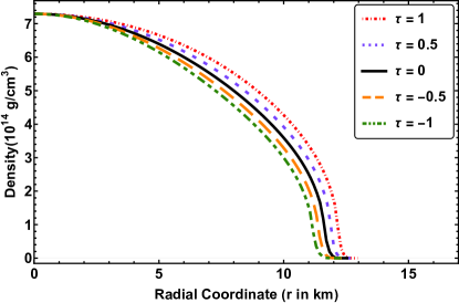
Figure 6: The density profiles inside neutron stars for various values of the anisotropic strength, each for $\rho_{c}=7.2955\times 10^{14}~{}{\rm g\,cm^{-3}}$ and BSk21 EoS.

In Fig. 7, we plot the radial coordinate (in km) inside the neutron star along the abscissa and the corresponding pressure along the ordinate for BSk21 EoS and different values of $\tau$. The left panel of the figure has the radial pressure along the ordinate while the right panel has the tangential pressure along the ordinate for the same values of $\tau$. Both of the plots are for $\rho_{c}=7.2955\times 10^{14}~{}{\rm g\,cm^{-3}}$. We see that for all values of $\tau$, both $p_{r}$ and $p_{t}$ decreases monotonically with the increase of $r$ and eventually reaches zero at the surface of the star.

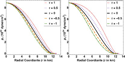
Figure 7: The variation of the radial (left panel) and the tangential (right panel) pressure inside neutron stars for various values of the anisotropic strength, each for $\rho_{c}=7.2955\times 10^{14}~{}{\rm g\,cm^{-3}}$ and BSk21 EoS.

III f-mode Oscillations of anisotropic neutron stars

III.1 Analytical Setup

To derive the differential equations governing the f-mode oscillations of neutron stars in general relativity, we have to take into account the perturbations in the metric as well as in the matter in the neutron star. First, we decompose the perturbed metric into two parts, a background and a perturbation on the background. So, the perturbed metric can be written as:

$$g_{\mu\nu}=g_{\mu\nu}^{(B)}+h_{\mu\nu},$$ (17)

where $g_{\mu\nu}^{(B)}$ is the background metric for the spherically symmetric static star, described in Eq. (1), and $h_{\mu\nu}$ is the perturbation on it up to the linear order. The linear order perturbation of the static spherically symmetric metric is decomposed into spherical harmonics $Y^{m}_{l}(\theta,\phi)$ and a function that has a radial dependence. The perturbed metric is accompanied by a perturbation in the energy-momentum tensor. The coupling between the perturbation of the metric and the perturbation in the energy-momentum tensor is described by the linearized perturbed Einstein equations,

$$\delta G_{~{}\alpha}^{\beta}=8\pi\delta T_{~{}\alpha}^{\beta},$$ (18)

where $\delta G_{~{}\alpha}^{\beta}$ is the perturbed Einstein tensor and $\delta T_{~{}\alpha}^{\beta}$ is the perturbed energy-momentum tensor. $G_{~{}\alpha}^{\beta}$ and $T_{~{}\alpha}^{\beta}$ are the un-perturbed Einstein tensor and the energy-momentum tensor, respectively. The expression of the linearized perturbed Einstein tensor, $\delta G_{\mu\nu}$, is given by [52],

$$\begin{split}{\delta G_{\mu\nu}}=-\frac{1}{2}[\nabla^{\alpha}\nabla_{\alpha}h_{\mu\nu}-(\nabla_{\nu}f_{\mu}+\nabla_{\mu}f_{\nu})+2{{{\mathcal{R}^{\alpha}}_{\mu}}^{\beta}}_{\nu}h_{\alpha\beta}+\nabla_{\nu}\nabla_{\mu}{{h^{\alpha}}_{\alpha}}-({\mathcal{R}^{\alpha}}_{\nu}h_{\mu\alpha}+{\mathcal{R}^{\alpha}}_{\mu}h_{\nu\alpha})+\\ g^{(B)}_{\mu\nu}(\nabla^{\alpha}f_{\alpha}+\nabla^{\beta}\nabla_{\beta}{h^{\alpha}}_{\alpha})+\mathcal{R}h_{\mu\nu}-g^{(B)}_{\mu\nu}\mathcal{R}^{\alpha\beta}h_{\alpha\beta}],\end{split}$$ (19)

where $f_{\nu}=\nabla^{\beta}h_{\nu\beta}$ and $\mathcal{R}_{\alpha\beta\gamma\delta}$, $\mathcal{R}_{\alpha\beta}$, and $\mathcal{R}$ are Riemann tensor, Ricci tensor, and Ricci scalar, respectively, of the background metric and $\nabla_{\sigma}$ denotes the covariant derivative along any coordinate $x^{\sigma}$. In the present work, we restrict ourselves to even parity perturbation (polar modes) for fixed values of $l$ and $m$. In Regge-Wheeler gauge [53], the even mode of perturbation takes the form:

$$h_{\alpha\beta}=-r^{l}\begin{pmatrix}e^{\nu}H_{0}(r)&i\omega rH_{1}(r)&0&0\\ i\omega rH_{1}(r)&e^{\lambda}H_{2}(r)&0&0\\ 0&0&r^{2}K(r)&0\\ 0&0&0&r^{2}\sin^{2}\theta K(r)\end{pmatrix}Y_{l}^{m}(\theta,\phi)e^{i\omega t}~{},$$ (20)

where $H_{0}(r)$, $H_{1}(r)$, $H_{2}(r)$, $K(r)$ are metric perturbation functions, that have only radial dependence, and $\omega$ is the angular frequency of the time varying component of the perturbation. We can further reduce the independent components of the metric perturbation. If we subtract the $``33"$ component of the Einstein equation from the $``22"$ component, we get the following:

$$\delta(G_{~{}2}^{2}-G_{~{}3}^{3}) =8\pi\delta(T_{~{}2}^{2}-T_{~{}3}^{3})$$ (21a)

$$=8\pi(\delta p_{t}-\delta p_{t})$$ (21b)

$$=0~{},$$ (21c)

where we have used the fact that $T_{~{}\alpha}^{\beta}=diag(-\rho,p_{r},p_{t},p_{t})$. The left hand side of the equation can easily be calculated from Eq. (19). After some algebra, we find that $H_{0}(r)=H_{2}(r)$. Hereafter, we will write $H_{0}(r)=H_{2}(r)=H(r)$.

After defining the metric perturbation, now we focus on the perturbation of the matter of the neutron star. The perturbation of the fluid in the star is described by the Lagrangian displacement vector $\xi^{\alpha}$, which has components [54, 31, 24] as follows:

$$\xi^{\mu}=\begin{pmatrix}0\\ r^{l-1}\,e^{-\lambda/2}W(r)\\ -r^{l-2}\,V(r){\partial}_{\theta}\\ -\frac{r^{l-2}}{\sin^{2}\theta}\,V(r){\partial}_{\phi}\end{pmatrix}Y_{l}^{m}(\theta,\phi)e^{i\omega t},$$ (22)

where $V(r)$ and $W(r)$ are fluid perturbation functions. We will use this Lagrangian displacement vector extensively to describe the perturbation of the energy-momentum tensor. The Lagrangian variation of the four velocity ($u^{\mu}$) can be written as [55]:

$$\Delta u^{\mu}=\frac{1}{2}u^{\mu}u^{\nu}u^{\sigma}\Delta g_{\nu\sigma},$$ (23)

where the Lagrangian perturbation of the metric is

$$\Delta g_{\alpha\beta}=h_{\alpha\beta}+\nabla_{\alpha}\xi_{\beta}+\nabla_{\beta}\xi_{\alpha}~{}.$$ (24)

These Lagrangian perturbations are related to Eulerian perturbations by the relation

$$\Delta=\delta+\mathcal{L}_{\xi},$$ (25)

where $\delta$ denotes the Eulerian variation and $\mathcal{L}_{\xi}$ is the Lie derivative along $\xi^{\alpha}$. The explicit expression for the Eulerian variation of the velocity four vector is given by

$$\delta u^{\mu}=(\delta^{\mu}_{~{}\rho}+u^{\mu}u_{\rho})(u^{\sigma}\nabla_{\sigma}\xi^{\rho}-\xi^{\sigma}\nabla_{\sigma}u^{\rho})+\frac{1}{2}u^{\mu}u^{\sigma}u^{\rho}h_{\sigma\rho}.$$ (26)

After substituting the expressions of $u^{\sigma}$, $\xi^{\sigma}$ and $h_{\alpha\beta}$ to Eq. (26), we get

$$\delta u^{\sigma}=\begin{pmatrix}-\frac{H}{2}\\ i\omega r^{-1}\,e^{-\lambda/2}W(r)\\ -i\omega r^{-2}\,V(r)\partial_{\theta}\\ -i\omega(r\sin\theta)^{-2}\,V(r)\partial_{\phi}\end{pmatrix}r^{l}e^{-\nu/2}Y_{l}^{m}(\theta,\phi)e^{i\omega t}.$$ (27)

We also expand the perturbation of the radial unit vector, $s^{\mu}$, in harmonics as follows:

$$\delta s^{\sigma}=\begin{pmatrix}i\omega S_{0}(r)\\ S_{1}(r)\\ 0\\ 0\end{pmatrix}r^{l}\,Y_{l}^{m}(\theta,\phi)\,e^{i\omega t},$$ (28)

where $S_{0}(r)$ and $S_{1}(r)$ are two functions of the radial coordinates, which we need to determine. For the sake of brevity, we will drop the independent variables (coordinates) from the functions for the rest of the paper, i.e., instead of $H(r)$, $H_{1}(r)$, $K(r)$, $W(r)$, $V(r)$, $S_{0}(r)$, $S_{1}(r)$, and $Y_{l}^{m}(\theta,\phi)$, we will simply write $H$, $H_{1}$, $K$, $W$, $V$, $S_{0}$, $S_{1}$, and $Y_{l}^{m}$, respectively.

As $s^{\sigma}$ is a space-like unit radial vector, so, up to the linear order, it should satisfy, $\delta s^{\sigma}s_{\sigma}+s^{\sigma}\delta s_{\sigma}=0$, as well as $\delta s^{\sigma}u_{\sigma}+s^{\sigma}\delta u_{\sigma}=0$. These two conditions allow us to write $S_{0}$ and $S_{1}$ as,

$$S_{0} = \frac{e^{-\nu}}{r}W-e^{-(\nu+\lambda/2)}\,r\,H_{1}~{},$$ (29)

$$S_{1} = \frac{e^{-\lambda/2}}{2}H~{}.$$ (30)

Now, to describe the perturbation in the density and the pressures (both the radial and the tangential), we need to know the perturbation of the number density. The Lagrangian perturbation in the number density of the particles can be derived from the conservation of the number density current, which is given by $\nabla_{\alpha}n^{\alpha}=0$, where $n^{\alpha}=nu^{\alpha}$, and $n$ is the number density of the particles. The Lagrangian perturbation in the number density of particles in the neutron star is given by [55, 56]:

$$\Delta n=-\frac{1}{2}n\perp^{\mu\nu}\Delta g_{\mu\nu}~{},$$ (31)

where $\perp^{\mu\nu}$ is the projection operator, which is orthogonal to the fluid flow. $\perp^{\mu\nu}$ can be expressed as:

$$\perp^{\mu\nu}=u^{\mu}u^{\nu}+g^{\mu\nu}.$$ (32)

Computing explicitly, we can write the expression of $\Delta n$ as,

$$\Delta n=-\frac{1}{2}n\perp_{g}Y^{m}_{l}e^{i\omega t},$$ (33)

where,

$$\perp_{g}=-2r^{l} \Bigg{[} \Bigg{(}K+\frac{1}{2}H\Bigg{)}-\frac{l(l+1)}{r^{2}}V$$ (34)

$$- \frac{e^{-\lambda/2}}{r}W^{\prime}-\Bigg{(}\frac{l+1}{r^{2}}e^{-\lambda/2}\Bigg{)}W\Bigg{]},$$

which is similar to the expression described by Comer et al. [25]. In our work, we consider the matter to be barotropic, where the density $(\rho)$ is a function of the number density only, i.e., $\rho=\rho(n)$. Hence, the perturbation in the density can be written as,

$$\Delta\rho=\frac{d\rho}{dn}\Delta n=\kappa\Delta n,$$ (35)

where $\kappa$ is the chemical potential $(\kappa=d\rho/dn)$. Now we can use the Gibbs relation, which is given by [55]:

$$\rho+p=\kappa n~{},$$ (36)

where the average pressure $p$ can be written as [57]:

$$p=\frac{1}{3}\left(T_{~{}1}^{1}+T_{~{}2}^{2}+T_{~{}3}^{3}\right)=\frac{p_{r}+2p_{t}}{3}=p_{r}+\frac{2}{3}\chi.$$ (37)

Note that, $p$ is the average over the directions and a function of the radial coordinate inside the star. Following the convention of this paper, we write $p$ instead of $p(r)$. Using Eq. (33) in Eq. (35) and the Gibbs relation, we get,

$$\Delta\rho=-\frac{1}{2}(p+\rho)\perp_{g}Y^{m}_{l}e^{i\omega t}~{}.$$ (38)

The Lagrangian variation of the radial pressure can be written as:

$$\Delta p_{r}=\frac{dp_{r}}{d\rho}\Delta\rho=-\frac{1}{2}\frac{dp_{r}}{d\rho}(p+\rho)\perp_{g}Y^{m}_{l}e^{i\omega t}~{}.$$ (39)

From the relation between the Lagrangian and the Eulerian variations, i.e., Eq. (25), we can write the relation between the Lagrangian perturbation and the Eulerian perturbation of the radial pressure as:

$$\Delta p_{r} =\delta p_{r}+\xi^{r}p^{\prime}_{r}$$

$$=\delta p_{r}+r^{l-1}\,e^{-\lambda/2}\left[-\frac{\nu^{\prime}}{2}(\rho+p_{r})+\frac{2\chi}{r}\right]W\,Y_{l}^{m}e^{i\omega t}.$$

From Eqs. (39) and (III.1), we get the expression for the Eulerian variation of the radial pressure, $\delta p_{r}$. With the help of $\delta p_{r}$, we calculate the Eulerian variation of $\rho$ and $p_{t}$, which are given by:

$$\delta\rho = \frac{d\rho}{dp_{r}}\delta p_{r},$$ (41)

$$\delta p_{t} = \delta\chi+\delta p_{r}.$$ (42)

With these expressions in our hand, we are ready to calculate the perturbation of the energy-momentum tensor, namely $\delta T_{~{}\alpha}^{\beta}$, which can be written as:

$$\delta T_{~{}\alpha}^{\beta}=(\delta\rho+\delta p_{t})u^{\beta}u_{\alpha}+(\rho+p_{t})(u^{\beta}\delta u_{\alpha}+\delta u^{\beta}u_{\alpha})$$

$$+\delta_{~{}\alpha}^{\beta}\delta p_{t}+(\delta p_{r}-\delta p_{t})s^{\beta}s_{\alpha}+(p_{r}-p_{t})(s^{\beta}\delta s_{\alpha}+\delta s^{\beta}s_{\alpha})~{}.$$ (43)

Using Eqs. (27), (28), and (III.1), as well as $u^{\beta}$ and $s^{\beta}$, we can calculate the non-zero components of the perturbed energy-momentum tensor, which are given by:

$$\delta T_{~{}0}^{0} =-\delta\rho=-\delta\tilde{\rho}(r)\,r^{l}Y_{l}^{m}e^{i\omega t}~{},$$ (44a)

$$\delta T_{~{}0}^{1} =-i\omega e^{-\lambda/2}r^{-1}[p_{r}+\rho]Wr^{l}Y_{l}^{m}e^{i\omega t}~{},$$ (44b)

$$\delta T_{~{}0}^{2} =i\omega r^{-2}[p_{r}+\rho+\chi]Vr^{l}\partial_{\theta}Y_{l}^{m}e^{i\omega t}~{},$$ (44c)

$$\delta T_{~{}0}^{3} =i\omega r^{-2}[p_{r}+\rho+\chi]Vr^{l}(\sin\theta)^{-2}\partial_{\phi}Y_{l}^{m}e^{i\omega t}~{},$$ (44d)

$$\delta T_{~{}1}^{1} =\delta p_{r}=\delta\tilde{p}_{r}(r)\,r^{l}Y_{l}^{m}e^{i\omega t}~{},$$ (44e)

$$\delta T_{~{}2}^{2} =\delta p_{t}=[\delta\tilde{p}_{r}(r)+\delta\tilde{\chi}(r)]\,r^{l}Y_{l}^{m}e^{i\omega t}~{},$$ (44f)

$$\delta T_{~{}3}^{3} =\delta p_{t}=[\delta\tilde{p}_{r}(r)+\delta\tilde{\chi}(r)]\,r^{l}Y_{l}^{m}e^{i\omega t}~{},$$ (44g)

where $\delta\rho$, $\delta p_{r}$ and $\delta\chi$ are decomposed into radial, angular and temporal parts as, $\delta\rho=r^{l}\,\delta\tilde{\rho}(r)\,Y_{l}^{m}e^{i\omega t}$, $\delta p_{r}=r^{l}\,\delta\tilde{p_{r}}(r)\,Y_{l}^{m}e^{i\omega t}$ and $\delta\chi=r^{l}\,\delta\tilde{\chi}(r)\,Y_{l}^{m}e^{i\omega t}$. In the above expressions, if we set $\chi=0$ and $\delta\chi=0$, the resulting expressions would resemble those of the isotropic case described by Thorne and Campolattaro [22].

Now, we use the linearly perturbed Einstein equations (Eq. (18)), and the equation of conservation of the energy-momentum tensor up to the linear order, i.e., $\delta(\nabla_{\nu}T^{\mu\nu})=0$, to derive equations of oscillation for the metric perturbation variables ($H$, $H_{1}$, $K$) as well as the fluid perturbation variables ($V$ and $W$). First, we perform a change of variable, which simplify the boundary condition. We know that, at the surface of the star $(r=R)$, the Lagrangian perturbation of the radial pressure is zero, i.e., $\Delta p_{r}=0$. We introduce a new variable $X$ to write $\Delta p_{r}$ in the form

$$\Delta p_{r}=-r^{l}e^{-\nu/2}XY_{l}^{m}e^{i\omega t}.$$ (45)

This change of variable allows us to write one of the perturbation equations in terms of $X$, and we can impose the boundary condition $X=0$ at $r=R$, when solving the oscillation equations numerically. Using the expressions from equations (34), (39), and (45), we extract the expression of $X$, which is given by:

$$X=(\rho + p)v_{sr}^{2}\Big{[}\frac{e^{\nu/2-\lambda/2}}{r}W^{\prime}+\frac{(l+1)e^{\nu/2-\lambda/2}}{r^{2}}W$$ (46)

$$+\frac{l(l+1)e^{\nu/2}}{r^{2}}V-e^{\nu/2}K-\frac{e^{\nu/2}}{2}H\Big{]},$$

where $v_{sr}^{2}=dp_{r}/d\rho$ and $p=p_{r}+(2\chi/3)$, as already defined. Using Eqs. (37), (39), (III.1), and (46), we can write the Eulerian perturbation of the radial pressure as:

$$\delta p_{r}=\delta\tilde{p}_{r}r^{l}Y_{l}^{m}e^{i\omega t}=\bigg{[} -e^{-\nu/2}X+\frac{1}{2r^{2}}e^{-\lambda/2}(-4\chi$$

$$+r\nu^{\prime}(p_{r}+\rho))W\bigg{]}r^{l}Y_{l}^{m}e^{i\omega t}~{}.$$ (47)

It is obvious that $X$ depends only on the radial coordinate $r$ and following the convention of this paper we write it simply as $X$. Using this new variable $X$, we write the governing equations of oscillations as:

$$H_{1}^{\prime} =\frac{e^{\lambda}}{r}H+\frac{e^{\lambda}}{r}K-\frac{(l+1)+2mr^{-1}e^{\lambda}+4\pi r^{2}e^{\lambda}(p_{r}-\rho)}{r}H_{1}-\frac{16\pi e^{\lambda}(\rho+p_{r}+\chi)}{r}V,$$ (48)

$$K^{\prime} =\frac{1}{r}H-\left[(l+1)r^{-1}-\frac{1}{2}\nu^{\prime}\right]K+\frac{l(l+1)}{2r}H_{1}-\frac{8\pi e^{\lambda/2}(p_{r}+\rho)}{r}W,$$ (49)

$$W^{\prime} =\frac{1}{2}e^{\lambda/2}rH+e^{\lambda/2}rK-\frac{e^{\lambda/2}l(l+1)}{r}V-\frac{(l+1)}{r}W+\frac{re^{\frac{\lambda-\nu}{2}}}{v_{sr}^{2}\left(p_{r}+\rho+\frac{2\chi}{3}\right)}X,$$ (50)

$$X^{\prime} =-2\frac{e^{\nu/2}}{r}\delta\tilde{\chi}-\left[\frac{l}{r}+\frac{\chi(6+r\nu^{\prime})}{rv_{sr}^{2}(3(p_{r}+\rho)+2\chi)}\right]X+(p_{r}+\rho)e^{\nu/2}\left[\frac{1}{2r}-\frac{\nu^{\prime}}{4}\right]H$$

$$\quad-\left[\frac{e^{\nu/2}l(l+1)(p_{r}+\rho)\nu^{\prime}}{2r^{2}}-\chi\frac{2l(l+1)e^{\nu/2}}{r^{3}}\right]V$$

$$\quad+\left[\frac{e^{\nu/2}(p_{r}+\rho)}{2}\left(\frac{l(l+1)}{2r}+r\omega^{2}e^{-\nu}\right)+\frac{\chi e^{\nu/2}l(l+1)}{2r}\right]H_{1}$$

$$\quad+\left[\frac{1}{2}e^{\nu/2}(p_{r}+\rho)\left(\frac{3}{2}\nu^{\prime}-\frac{1}{r}\right)+\chi\frac{e^{\nu/2}(-6+r\nu^{\prime})}{2r}\right]K$$

$$\quad+\left[-\frac{e^{\nu/2}(p_{r}+\rho)}{r}\left(e^{\lambda/2-\nu}\omega^{2}+4\pi e^{\lambda/2}(p_{r}+\rho)-\frac{1}{2}r^{2}(r^{-2}e^{-\lambda/2}\nu^{\prime})^{\prime}\right)\right.$$

$$\quad\left.-\chi^{\prime}\frac{2e^{(\nu-\lambda)/2}}{r^{2}}+\frac{e^{(\nu+\lambda)/2}}{r^{3}}\chi\left(6-14mr^{-1}-8\pi r^{2}p_{r}\right)\right]W,$$ (51)

where $H_{1}$ and $K$ were introduced in Eq. (20), $W$ in Eq. (22), and $X$ in (Eq. 45). The remaining functions in Eq. (20) and (22), namely $H_{0}=H_{2}=H$ and $V$ are related to other functions by following algebraic relations:

$$\Biggl{[}3m +\frac{1}{2}(l-1)(l+2)r+4\pi r^{3}p_{r}\Biggr{]}H=8\pi e^{-\nu/2}r^{3}X-\Biggl{[}-e^{-\nu-\lambda}r^{3}\omega^{2}+\frac{1}{2}l(l+1)(m+4\pi r^{3}p_{r})\Biggr{]}H_{1}$$ (52)

$$\quad+\chi 16e^{-\lambda/2}\pi rW-\Biggl{[}-\frac{1}{2}(l-1)(l+2)r+e^{-\nu}r^{3}\omega^{2}+\frac{e^{\lambda}}{r}(m+4\pi r^{3}p_{r})(3m-r+4\pi r^{3}p_{r})\Biggr{]}K,$$

$$\omega^{2}(\rho+p_{r}+\chi)V=e^{\nu/2}X-\frac{1}{2}e^{\nu}(p_{r}+\rho)H+\frac{e^{\nu-\lambda/2}p^{\prime}_{r}}{r}W-e^{\nu}\delta\tilde{\chi}~{}.$$ (53)

These are the set of equations that govern the oscillations of anisotropic neutron stars in general relativity. The equations for the metric perturbation dynamics, i.e., $H_{1}^{\prime}$ is obtained from $\delta G_{~{}0}^{2}=8\pi\delta T_{~{}0}^{2}$ and the equation for $K^{\prime}$ is obtained from $\delta G_{~{}0}^{1}=8\pi T_{~{}0}^{1}$. $\delta G_{~{}\nu}^{\mu}$ is obtained by putting $h_{\mu\nu}$ from Eq. (20) in Eq. (19) and raising one index. The explicit expressions for $\delta T_{~{}\mu}^{\nu}$ is given in Eq. (44). On the other hand, the dynamics of the fluid perturbations, which are given by $W^{\prime}$ and $X^{\prime}$, are obtained with the help of Eq. (46) and $\delta(\nabla_{\mu}T_{~{}\,1}^{\mu})=0$, respectively. Eq. (52), which relates the metric perturbation variable $H$ with other variables, has been obtained by combining $\delta G_{~{}1}^{1}=8\pi T_{~{}1}^{1}$ and $\delta G_{~{}1}^{2}=8\pi\delta T_{~{}1}^{2}$. Eq. (53) relates the fluid perturbation variable $V$ with other variables and has been obtained from $\delta(\nabla_{\mu}T_{~{}\,2}^{\mu})=0$. The effect of anisotropy is manifested in these equations through terms having $\chi$, $\chi^{\prime}$, and $\delta\chi$. These terms are zero in the isotropic case and our equations take the well known forms given by Detweiler and Lindblom [24].

For the choice of our ansatz of anisotropy, we get

$$\delta\chi=\frac{\partial\chi}{\partial p_{r}}\delta p_{r}+\frac{\partial\chi}{\partial\mu}\delta\mu~{}.$$ (54)

Note that, unlike Cowling approximation, in our full general relativistic framework, the variable $\mu$ is perturbed. The quantity $\mu=2m/r=1-e^{-\lambda}$, which describes the local compactness of the star, can be perturbed as $\delta\mu=\lambda e^{\lambda}\delta\lambda$, where $\delta\lambda$ represents the perturbation of $\lambda$. As we are interested up to the linear order perturbation, so from the perturbation of the metric, we can write,

$$e^{\lambda+\delta\lambda}=e^{\lambda}(1-Hr^{l}Y_{l}^{m}e^{i\omega t})~{}.$$ (55)

Neglecting the higher order perturbation terms (O$((\delta\lambda)^{2})\dots$), we can write,

$$\delta\lambda=-Hr^{l}Y_{l}^{m}e^{i\omega t}~{}.$$ (56)

Using Eqs. (15), (44e), and (56) in Eq. (54), we get

$$\delta\chi=\tau\left[\left(\frac{2m}{r}\right)\delta\tilde{p}_{r}-\left(p_{r}\left(1-\frac{2m}{r}\right)H\right)\right]r^{l}Y_{l}^{m}e^{i\omega t}~{},$$ (57)

where $\delta\tilde{p}_{r}$ is given in equation (III.1).

III.2 Numerical Techniques

Equipped with the above set of equations, we are now prepared to solve them numerically. Since our primary objective is to determine the quasi-normal modes, it is important to carefully consider the specific initial value and boundary value conditions. In contrast to the background case, here we are confronted with the task of handling seven first-order differential equations (three for the background and four for the perturbations) as well as two simultaneous algebraic relations. It is crucial to ensure that the equations remain regular at the center of the star, while the boundary condition dictates that the Lagrangian perturbation of the radial pressure $(\Delta p_{r})$ must be zero at the outermost surface of the perturbed star. By examining the set of equations, we observe that they exhibit singularity at $r=0$. In order to ensure regularity at the center, we expand all the variables at a point $r=R/10^{6}$ as a Taylor series around $r=0$. The variables for which we do such expansions include the variables that describe the unperturbed star, e.g., $\lambda$, $\nu$, $m$, $\rho$, $p_{r}$, $\chi$ as well as the perturbation variables $H$, $H_{1}$, $K$, $V$, $W$, and $X$. We substitute these expansions into the equations that govern the unperturbed star (Eqs. (9), (12), (13)), as well as perturbation equations (Eqs . (48), (49), (50), (51), (52), and (53)) to derive the necessary conditions that are:

$$H_{1}(0) =\frac{1}{l(l+1)}\left[2lK(0)+16\pi\left\{\rho(0)+p_{r}(0)\right\}W(0)\right],$$ (58)

$$X(0) =\left\{p_{r}(0)+\rho(0)\right\}\,e^{\nu(0)/2}\left[\left\{\frac{4\pi}{3}\left\{\rho(0)+3p_{r}(0)\right\}\right.\right.$$

$$\quad\left.\left.-\frac{\omega^{2}e^{-\nu(0)}}{l}\right\}W(0)+\frac{1}{2}K(0)\right]-e^{\nu(0)/2}\chi_{2}(0)W(0),$$ (59)

where $\chi_{2}(0)$ is the second order in the expansion of $\chi(r)$. Since the radial and the tangential pressures are equal at the center, we have $\chi(0)=\delta\chi(0)=0$. This condition guarantees that at the center, the radial pressure is equal to the tangential pressure, and the Eulerian perturbation of the radial pressure is equal to the Eulerian perturbation of the tangential pressure. Based on our ansatz (Eq.(15)), we can express $\chi_{2}(0)$ as $\chi_{2}(0)=\tau\frac{16\pi}{3}\rho(0)p_{r}(0)$. From Eqs. (58) and (59), we see that $H_{1}(0)$ and $X(0)$ depend on two independent variables $K(0)$ and $W(0)$. These expressions exhibit similarity to those of the isotropic case described by Detweiler and Lindblom [24], with the addition of the term containing $\chi_{2}(0)$ that arises due to the presence of the anisotropy. Now, we need to set the values of $W(0)$ and $K(0)$ in such a way that after integrating Eqs. (48), (49), (50), (51), (52), and (53) along with Eqs. (9), (12), (13), radially outward from the point $R/10^{6}$, we would get $X(R)=0$. To do this, following Lindblom and Detweiler [23], we use two sets of values of $W(0)$ and $K(0)$, namely, $W(0)=1$, $K(0)=+[\rho(0)+p_{r}(0)]$ and $W(0)=1$, $K(0)=-[\rho(0)+p_{r}(0)]$. We perform outward integration with each of the sets independently and get two independent values of $X$ at $r=R$, say $X_{+}$ and $X_{-}$. Then, we combine these two solutions as $X(R)=c_{+}X_{+}+c_{-}X_{-}$ and choose the values of the coefficients $c_{+}$ and $c_{-}$ to ensure $X(R)=0$.

For the integration process, we have employed the ‘LSODA’ [58, 59] method of integration, which dynamically switches between the BDF (Backward Differentiation Formula) method and the Adams method based on the stiffness of the coupled equations. In our implementation, we have set both the relative and the absolute tolerances to $10^{-10}$. This completes the integration inside the neutron star.

Outside the star, all the fluid perturbation variables become zero but the metric perturbation variables remain non-zero. This results in a reduction of the number of the equations to two, specifically, the equations for $H_{1}^{\prime}$ and $K^{\prime}$. Following the standard technique, we now perform a transformation of variables given by

$$r^{l}K =\frac{n_{l}(n_{l}+1)r^{2}+3n_{l}Mr+6M^{2}}{r^{2}(n_{l}r+3M)}Z+\frac{dZ}{dr^{*}},$$ (60)

$$r^{l+1}H_{1} =\frac{n_{l}r^{2}-3n_{l}Mr-3M^{2}}{(r-2M)(n_{l}r+3M)}Z+\frac{r^{2}}{(r-2M)}\frac{dZ}{dr^{*}},$$ (61)

where $n_{l}=[l(l+1)/2]-1$, and $r^{*}=r+2M\,\ln[(r/2M)-1]$. With these transformations, the differential equations for $H_{1}^{\prime}$ and $K^{\prime}$ can be combined into a single second order differential equation as:

$$\frac{d^{2}}{dr^{*2}}\left\{Z(r^{*})\right\}\,+\left[\omega^{2}-V_{z}(r^{*})\right]Z(r^{*})=0,$$ (62)

where,

$$V_{z}(r^{*})=\frac{(1-2M/r)}{r^{3}(n_{l}r+3M)^{2}}\left[2n_{l}^{2}(n_{l}+1)r^{3}+6n_{l}^{2}Mr^{2}\right.$$

$$\left.\quad+18n_{l}M^{2}r+18M^{3}\right].$$ (63)

Equation (62) is known as the Zerilli equation, which was first derived by Zerilli [60] for the Schwarzschild geometry. The variable $Z(r^{*})$ is known as the Zerilli function, which we usually simply write as $Z$. This methond was later used by Lindblom and Detweiler [23] first time specifically for neutron stars.

To determine the quasi-normal modes, it is necessary to identify the frequencies for which the Zerilli equation satisfies the condition for a purely outgoing wave at the spatial infinity. For this purpose, one needs to numerically integrate the Zerilli equation from the surface of the star ($r=R$) to spatial infinity. In our numerical implementation, we have performed the integration up to a distance of $50~{}\omega^{-1}$, as the values of $Z$ and $dZ/dr^{*}$ take the asymptotic values at that distance [23, 61]. Here $\omega$ is the angular frequency of the oscillation as introduced in Eq. (20). In the large $r$ limit, the solution of the Zerilli equation can be assumed to be purely sinusoidal, which can be interpreted as a composition of the ingoing and the outgoing waves. Denoting the ingoing wave as $Z_{in}(r^{*})$ and the outgoing wave as $Z_{out}(r^{*})$, we can write the solution at in the large $r$ limit as:

$$Z(r^{*})=B_{in}Z_{in}(r^{*})+B_{out}Z_{out}(r^{*}),$$ (64)

where $B_{in}$ and $B_{out}$ are the coefficients of $Z_{in}$ and $Z_{out}$, respectively, which determine the proportion of the in-going and the outgoing waves in the large $r$ limit and are complex conjugate to each other. In this limit limit, $Z_{in}(r^{*})$ and $Z_{out}(r^{*})$ can be assumed as power series, which can be written as:

$$Z_{out}(r^{*}) =e^{(-i\omega r^{*})}\sum_{j=0}^{\infty}\beta_{j}r^{-j}~{},$$ (65)

$$Z_{in}(r^{*}) =e^{(i\omega r^{*})}\sum_{j=0}^{\infty}\bar{\beta}_{j}r^{-j}~{},$$ (66)

where $\beta_{j}$s are the coefficients of the power series expansions, and $\bar{\beta}_{j}$s are the complex conjugate of $\beta_{j}$s. The coefficients $\beta_{j}$s can be obtained through a recursion relation by substituting equations (65) and (66) into equation (62). To determine the asymptotic behavior of $Z(r^{*})$, we consider the expansion up to $O(r^{-2})$. The relevant expressions are as follows:

$$\beta_{1} =-i\omega^{-1}(n_{l}+1)\beta_{0}~{},$$ (67)

$$\beta_{2} =-\frac{1}{2\omega^{2}}\left[n_{l}(n_{l}+1)-3iM\omega\left(1+\frac{2}{n_{l}}\right)\right]\beta_{0}~{},$$ (68)

where $\beta_{0}$ is an arbitrary constant. For numerical implementation, we have considered $\beta_{0}=p_{r}(0)/\rho(0)$, as suggested by Chandrasekhar and Ferrari [62]. This choice provides a convenient normalization for the coefficients $\beta_{j}$ in the recursion relation. From these expressions, we can observe that for a fixed mass of the neutron star and for a specific angular mode ($l=2$ in the present work), the coefficients $B_{in}$ and $B_{out}$ depend solely on the angular frequency $\omega$. To determine the numerical values of $B_{in}$ and $B_{out}$, we can compare the numerically integrated values of the Zerilli function and its first derivative with the corresponding asymptotic analytical values described above. By calculating $B_{in}$ for various frequencies, we can treat it as a function of $\omega$. Consequently, we can find the root of this function, which implies $B_{in}(\omega)=0$, i.e., purely outgoing wave for that particular $\omega$. The frequency of the oscillation is given by $\mathcal{F}={\rm Re}(\omega)/2\pi$ where ${\rm Re}(\omega)$ is the real part of the root. The inverse of the imaginary part of the root ($\rm 1/Im(\omega)$) is the damping time of the oscillation. The values of the mode frequency and corresponding damping time obtained by our code for $\tau=0$ agrees with earlier results reported by Lu and Suen [63] and Kunjipurayil et al. [29].

IV Results for f-mode oscillations of anisotropic neutron stars

In the preceding sections, we provided the details of the analytical and numerical procedures employed to determine the quasi-normal modes of anisotropic neutron stars. In this section, our main aim is to quantify these effects. As discussed earlier, in most of the cases, we use BSk21 EoS to solve the equations for the unperturbed stellar configuration as well as the oscillation of the stars, and in some cases, we compare the results with those obtained with a softer BSk19 EoS, to understand the effect of the softness of the EoS in the behavior of the quasi-normal modes in anisotropic neutron stars.

However, to achieve these, first we explore one additional aspect related to the structure of anisotropic stars. We present various physical parameters in Table-1. From this table as well as from Figs. 3 and 4, it is clear that for any fixed value of the anisotropic strength, at smaller values of the central density ($\rho_{c}$), an increase in the central density leads to simultaneous increases in the mass ($M$) and the radius ($R$) of the star, up to a certain threshold. In this region, the average density of the stars increases slowly, where the average density of the neutron star is given by $\rho_{\rm avg}=M[(4/3)\pi R^{3}]^{-1}$. As an example, for the $\tau=0$ case, this trend holds true up to about $\rho_{c}=8.2817\times 10^{14}~{}{\rm g\,cm^{-3}}$, which gives the mass of the star as $1.6~{}{\rm M_{\odot}}$. However, above this threshold value of the central density, for each value of the anisotropic strength, an increase in the value of the central density is accompanied by a decrease in the radius and an increase in the mass, resulting in a rapid growth in the average density. To demonstrate the manifestations of this phenomenon, in Fig. 8, we plot the values of the anisotropic strength along the horizontal axis and the values of the square root of the average density ($\sqrt{\rho_{\rm avg}}$) along the vertical axis for neutron stars of masses $1~{}{\rm M_{\odot}}$, $1.4~{}{\rm M_{\odot}}$, and $2.274~{}{\rm M_{\odot}}$. These masses represent a possible low mass for a neutron star, the commonly expected mass for a neutron star, and a possible high mass for a neutron star. Moreover, the high mass value ($2.274~{}{\rm M_{\odot}}$) is the maximum mass of a stable isotropic neutron star for this EoS. Stable neutron stars of mass $1~{}\rm M_{\odot}$ exist in the range of $-2\leq\tau\leq 2$, of mass $1.4~{}\rm M_{\odot}$ exist in the range of $-2\leq\tau\leq 1.9$, and of mass $2.274~{}\rm M_{\odot}$ exist in the range of $0\leq\tau\leq 1$. From Fig. 8, we see that if the value of $\tau$ increases from 0 to 1, the value of $\sqrt{\rho_{\rm avg}}$ decreases by $2.21\%$, $3.30\%$, and $18.86\%$ for the neutron stars of masses $1~{}{\rm M_{\odot}}$, $1.4~{}{\rm M_{\odot}}$, and $2.274~{}{\rm M_{\odot}}$, respectively.

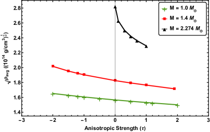
Figure 8: The change in the square root of the average density with the anisotropic strength for various masses of neutron stars for BSk21 EoS.

Table 1: Numerical values of various parameters for the BSk21 EoS. The columns from left to right contain the values of the anisotropic strength ($\tau$), the central density ($\rho_{c}$), the mass of the star ($M$), the radius ($R$), the average density ($\rho_{\rm avg}$), the f-mode frequency ($\mathcal{F}$), and the damping time.

Anisotropic Strength	Central Density $(\rm 10^{14}~{}g\,cm^{-3})$	Mass $\rm(M_{\odot})$	Radius (km)	Average Density $(\rm 10^{14}~{}g\,cm^{-3})$	f-mode Frequency (kHz)	Damping Time (ms)
0	5.7661	1.0	12.4664	2.4501	1.564112	430.098
0	6.4801	1.2	12.5459	2.8846	1.638928	313.507
0	7.2955	1.4	12.5893	3.3307	1.713102	243.028
0	8.2817	1.6	12.5801	3.8148	1.79002	197.672
0	9.5711	1.8	12.4969	4.3779	1.87431	167.387
0	11.4921	2.0	12.2946	5.1085	1.97585	149.81
0	22.6476	2.274	11.0593	7.98034	2.31740	154.28
0.5	5.5206	1.0	12.5623	2.3944	1.58505	396.74
0.5	6.1758	1.2159	12.6719	2.8365	1.6683	278.21
0.5	6.7874	1.4	12.7379	3.2155	1.7377	217.25
0.5	8.0285	1.7110	12.7625	3.9071	1.8580	155.94
0.5	9.1689	1.92551	12.6896	4.4731	1.94919	130.85
0.5	12.4966	2.274	12.2523	5.8688	2.14665	108.88
0.5	20.1137	2.4362	11.2095	8.210	2.4217	114.96
1	5.3021	1.0	12.6541	2.34272	1.60160	370.81
1	5.8204	1.2	12.7767	2.73106	1.67973	263.49
1	6.3670	1.4	12.8748	3.11398	1.75493	198.69
1	7.6519	1.8	12.9551	3.92969	1.90563	128.78
1	10.0875	2.274	12.7127	5.25396	2.11507	91.68
1	14.0191	2.55264	12.0033	7.00652	2.33588	85.39
-0.5	6.0447	1.0	12.3657	2.5104	1.5374	474.48
-0.5	6.9786	1.2172	12.4212	3.0149	1.6133	345.96
-0.5	7.9262	1.4	12.4258	3.4638	1.67739	281.40
-0.5	11.4870	1.8197	12.17058	4.7917	1.84762	208.40
-0.5	15.0573	2.0	11.7962	5.7837	1.9595	201.84
-0.5	16.05715	2.02851	11.6938	6.02173	1.985	203.134
-1	6.36435	1.0	12.2595	2.57629	1.50286	535.91
-1	7.12128	1.15	12.2799	2.9480	1.54874	438.04
-1	8.7378	1.4	12.2429	3.62151	1.62368	344.18
-1	10.6688	1.6	12.10918	4.27752	1.68731	307.82
-1	13.8956	1.78855	11.8161	5.14626	1.76009	302.63

Next, we investigate the the effect of the anisotropy on the quasi-normal f-mode of neutron stars. In Fig. 9, we plot the frequency of the f-mode along the abscissa and the square root of the average density along the ordinate. From the calculations within the Newtonian theory, we know that the f-mode frequency is proportional to the square root of the average density of a neutron star [64] even in the case with anisotropy [30]. From Fig. 9, we see that this frequency versus the square root of the average density ($\mathcal{F}-\sqrt{\rho_{\rm avg}}$) relation remains unchanged even when full general relativistic calculations are performed. The higher values of the anisotropic strength results in higher values of the slope of the $\mathcal{F}-\sqrt{\rho_{\rm avg}}$ lines. From this figure, it is clear that the f-mode frequency can be written as a functional form as:

$$\mathcal{F}(\rho_{\rm avg},\tau)\approx C\sqrt{\rho_{\rm avg}}\,g(\tau)~{},$$ (69)

where $C$ is a positive constant of proportionality, and $g(\tau)$ is a monotonically increasing function of $\tau$.

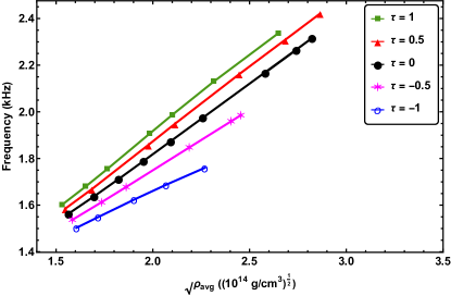
Figure 9: The variation of the f-mode frequency with the square root of the average density of the neutron stars for various values of the anisotropic strength for BSk21 EoS.

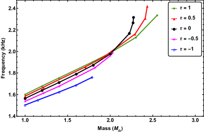
Figure 10: The variation of the f-mode frequency with the mass of neutron stars for various values of the anisotropic strength for BSk21 EoS.

In Fig. 10, we plot the frequencies against the mass of the neutron stars for several values of the anisotropic strength. From this figure, we see that, for any given value of the anisotropic strength, neutron stars of higher masses have higher values of the the f-mode frequency. For lower masses (less than about $2~{}{\rm M_{\odot}}$), the increase of the frequency with the mass is linear, but for massive stars, the frequency increases rapidly with the increase in the value of the mass. However, this non-linear rise in the frequency with the mass is not prominent for negative values of $\tau$. We also see that, for a fixed mass below about $2~{}{\rm M_{\odot}}$, a higher value of $\tau$ has a larger frequency, but above it, a higher value of $\tau$ corresponds to a lower frequency.

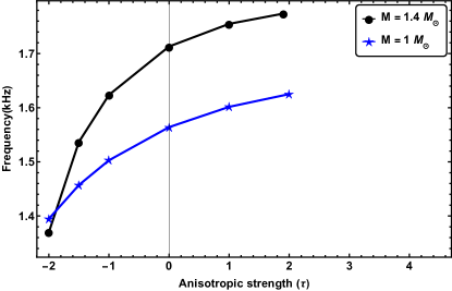
(a) Variation of the f-mode frequency with the anisotropic strength for near solar mass neutron stars.

(b) Variation of the f-mode frequency with the anisotropic strength for massive neutron stars.

.

Figure 11: Frequencies of f-modes for various anisotropic strengths for three different masses of neutron stars for BSk21 EoS.

The rapid increase in the values of the f-mode frequency with the mass for high values of masses (as seen in Fig. 10) can be understood from Eq. (69) and Fig. 8. Fig. 8 demonstrates the fact that for a fixed value of the anisotropic strength, the value of $\sqrt{\rho_{\rm avg}}$ increases if the mass of the neutron star increases, and this increase becomes faster for higher values of the mass. As an example, for $\tau=0$, if we change the mass of the neutron star from $1.0~{}{\rm M_{\odot}}$ to $1.4~{}{\rm M_{\odot}}$, i.e, $\Delta M=0.4~{}{\rm M_{\odot}}$, the value of $\sqrt{\rho_{\rm avg}}$ changes from $1.56\times 10^{7}~{}{\rm g^{1/2}\,cm^{-3/2}}$ to $1.82\times 10^{7}~{}{\rm g^{1/2}\,cm^{-3/2}}$, i.e., $\Delta\sqrt{\rho_{\rm avg}}=0.26\times 10^{7}~{}{\rm g^{1/2}\,cm^{-3/2}}$ giving $\Delta\sqrt{\rho_{\rm avg}}/\Delta M=0.65\times 10^{7}~{}{\rm g^{1/2}\,cm^{-3/2}\,M_{\odot}^{-1}}$. On the other hand, if we change the mass of the neutron star from $1.4~{}{\rm M_{\odot}}$ to $2.274~{}{\rm M_{\odot}}$ keeping $\tau$ fixed at 0, i.e, $\Delta M=0.874~{}{\rm M_{\odot}}$, the value of $\sqrt{\rho_{\rm avg}}$ changes from $1.82\times 10^{7}~{}{\rm g^{1/2}\,cm^{-3/2}}$ to $2.82\times 10^{7}~{}{\rm g^{1/2}\,cm^{-3/2}}$, i.e, $\Delta\sqrt{\rho_{\rm avg}}=1.0\times 10^{7}~{}{\rm g^{1/2}\,cm^{-3/2}}$ giving $\Delta\sqrt{\rho_{\rm avg}}/\Delta M=1.14\times 10^{7}~{}{\rm g^{1/2}\,cm^{-3/2}\,M_{\odot}^{-1}}$. As for a fixed value of $\tau$, the value of the f-mode frequency is proportional to $\sqrt{\rho_{\rm avg}}$, this explains why for $\tau=0$, although the rise in the value of the frequency with mass is linear for masses less than $2~{}{\rm M_{\odot}}$, for masses higher than $2~{}{\rm M_{\odot}}$, we see a rapid non-linear rise in the value of the frequency with the increase in the value of the mass, as seen in Fig. 10. Moreover, for each value of $\tau$, for smaller values of the mass, $g(\tau)$ dominates $\mathcal{F}(\rho_{\rm avg},\tau)$ of Eq. (69). Hence, higher values of $\tau$ give higher values of the frequency. On the other hand, for each value of $\tau$, for higher values of the mass, $\sqrt{\rho_{\rm avg}}$ dominates $\mathcal{F}(\rho_{\rm avg},\tau)$ of Eq. (69). Hence, higher values of $\tau$ give lower values of the frequency, because, for a fixed mass, $\sqrt{\rho_{\rm avg}}$ decreases with the increase in the value of $\tau$ as seen in Fig. 8.

To understand the effect of anisotropy on the f-mode frequency for a particular mass of the neutron star, in Fig. 11, we have plotted the frequency with respect to the anisotropic strength for the same three values of the mass that were used in Fig. 8. One point to note here is the fact that, $2.274~{}{\rm M_{\odot}}$ is above the threshold mass value above which a higher value of $\tau$ results in a lower value of the mode frequency for a fixed mass as seen in Fig. 10, while masses $1~{}{\rm M_{\odot}}$ and $1.4~{}{\rm M_{\odot}}$ are below that threshold.

From Fig. 11a, we see the fact that for neutron stars of masses $1~{}{\rm M_{\odot}}$ and $1.4~{}{\rm M_{\odot}}$, the frequency increases as the anisotropic strength increases. Comparing the f-mode frequency of an anisotropic star with $\tau=1.9$ and a mass of $1.4~{}{\rm M_{\odot}}$ to that of an isotropic star with the same mass, we observe an increase in the frequency of $3.62\%$. Similarly, comparing the frequency of an anisotropic stars with $\tau=-1.9$ and a mass of $1.4~{}{\rm M_{\odot}}$ to that of an isotropic star of the same mass, we see a decrease of $17.37\%$. The f-mode frequency of a $1~{}\rm{M_{\odot}}$ star with $\tau=2$ is $3.9\%$ higher compared to that of the isotropic stars of the same mass, whereas for $\tau=-2$ with the same mass, the frequency decreases by $10.8\%$ of that of an isotropic star of the same mass. On the other hand, for the neutron star of mass $2.274~{}\rm{M_{\odot}}$, the f-mode frequency decreases as the anisotropy inside the star increases. From Fig. 11b, we see that the frequency experiences a decrease of approximately $9.56\%$ as the anisotropic strength increases from $0$ to $1$. This characteristic, where an increase in the anisotropic strength leads to a decrease in the f-mode frequency, also exists in the framework of Cowling approximation [32].

The change in the frequency due to the change of the anisotropic strength ($\tau$) for different masses can be explained from Figs. 9 and 8. Fig. 9 shows that $g(\tau)$ of Eq. (69) is a monotonically increasing function of $\tau$. From Fig. 8, we see that while $\sqrt{\rho_{\rm avg}}$ decreases only marginally when $\tau$ increases from 0 to 1 for neutron stars of masses $1~{}\rm M_{\odot}$ and $1.4~{}\rm M_{\odot}$, it decreases substantially for neutron stars of masses $2.274~{}\rm M_{\odot}$. Hence, only in the last case, the decrease in the value $\sqrt{\rho_{\rm avg}}$ can surpass the increasing trend of $g(\tau)$ to result in a decrease in the value of the f-mode frequency with the increase in the value of $\tau$.

Next, we explore the influence of the stiffness of the EoS on the f-mode frequency. We plot the frequency as a function of the anisotropic strength for both the BSk19 and BSk21 EsoS in Fig. 12. To facilitate a direct comparison of the stiffness effect, we considered a fixed mass $1.4~{}{\rm M_{\odot}}$ for the neutron stars for both of the EsoS. For BSk21 EoS, stable neutron stars of mass $1.4~{}{\rm M_{\odot}}$ can exist in the range of the anisotropic strength $-2\lesssim\tau\lesssim 1.9$, while for BSk19 EoS, this range is $-1\lesssim\tau\lesssim 1.5$. From the figure, we see that the qualitative nature of the two curves is similar, indicating a common trend. However, it is evident that the neutron stars with a softer EoS like the BSk19 EoS, exhibit higher frequencies of oscillations across the entire range of the anisotropy. Another point to notice here is the fact that, the influence of the anisotropy is less for the softer EoS (BSk19) with respect to the stiffer EoS (BSk21) when $\tau>0$.

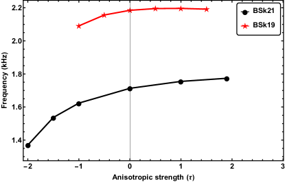
Figure 12: The variation of the f-mode frequency with the anisotropic strength for neutron stars of mass $1.4~{}\rm M_{\odot}$ for BSk19 and BSk21 EsoS.

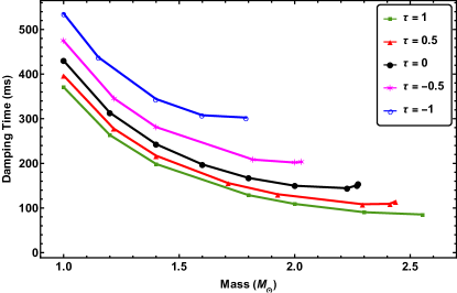
Figure 13: The variation of the damping time with the mass of the neutron stars for various values of the anisotropic strength for BSk21 EoS.

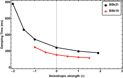
Figure 14: The variation of the damping time with the value of the anisotropic strength for neutron stars with the mass of $1.4~{}{\rm M_{\odot}}$ for BSk19 and BSk21 EsoS.

In addition to the mode frequency, another crucial aspect associated with the mode is the damping time. Hence, next we investigate the effect of the anisotropy on the damping time of the f-mode oscillation. In Fig. 13, we plot the values of the damping time against the mass of neutron stars for several values of the anisotropic strength. From this figure, we see that the damping time decreases as the mass of the neutron star increases for all values of the anisotropic strength. However, it is worth noting that for mildly anisotropic neutron stars, a slight increase in the damping time occurs near the stable maximum mass.

In Fig. 14, we plot the values of the anisotropic strength along the abscissa and the values of the damping time along the ordinate for neutron stars of a fixed mass $1.4~{}{\rm M_{\odot}}$ for EsoS BSk21 and BSk19. From the figure, we see that the qualitative nature of the two curves is similar, indicating a common trend. However, it is evident that the neutron stars with a softer EoS like the BSk19 EoS, gives smaller values of the damping time of oscillations across the entire range of the anisotropy. We also notice the fact that, for a neutron star with BSk21 EoS and an anisotropic strength of $\tau=2$, the damping time experiences a decrease of $28\%$ compared to an isotropic star of the same mass. Conversely, for the same BSk21 EoS, as the value of $\tau$ decreases from $0$ to $-2$, we observe a significant increase in the damping time, approximately three times ($300\%$) of that for the isotropic case. For neutron stars with BSk19 EoS, as the anisotropic strength increases from $0$ to $1.5$, the damping time decreases by $24\%$. Conversely, as the anisotropic strength decreases from $0$ to $-1$, the damping time increases by $60\%$.

V Summary and Conclusion

In this paper, we studied the effects of the anisotropy within neutron stars on the frequency and the damping time of the quasi-normal modes, as compared to those of isotropic neutron stars. To achieve this, we have employed the full framework of general relativity (up to the linear order perturbation), considering both the metric and the fluid perturbations to derive the oscillation equations. Notably, these equations share a similar structure to the isotropic counterparts but contain additional terms that account for the difference between the radial and the tangential pressure and its perturbations. As our focus lies on gravitational waves, we consider the specific case with $l=2$, although the equations can be applied to any value of $l$. Among varios $l=2$ modes, we have focused on studying the fundamental (f) modes of neutron stars, which typically span a frequency range of $1-3$ kHz. These modes are relatively easier to excite compared to other modes [65], and their analysis provides crucial insights into the oscillatory behavior and dynamic characteristics of neutron stars. In our analysis, we have demonstrated that the frequency of the f-mode exhibits a linear relationship with the square root of the average density of neutron stars, for both isotropic and anisotropic neutron stars. Importantly, the slope of the linear fit depends on the anisotropic strength $\tau$, increases with the increase of $\tau$ from zero, and decreases with the decrease of $\tau$ from zero. Such relation was obtained earlier within the Newtonian framework by Hillebrandt and Steinmetz [30].

As the mass of the neutron stars can be determined by observing them in the electromagnetic waves, we have plotted variations of the f-mode frequencies and the damping time with the mass of the star in Fig. 10 and Fig. 13 respectively. We have seen that, the qualitative nature of variations are the same for both the isotropic as well as the anisotropic stars. From Fig. 11, we see that for neutron stars of masses $1~{}{\rm M_{\odot}}$ and $1.4~{}{\rm M_{\odot}}$, the frequency increases with the increase in the anisotropic strength. But for a neutron star of mass $2.274~{}{\rm M_{\odot}}$, we found that the frequency decreases with the increase in the anisotropic strength. As discussed earlier, this feature is attributed to rapid decrease of the square root of the average density with the anisotropic strength for massive neutron stars and very slow decrease of the square root of the average density with the anisotropic strength for neutron stars of masses near the solar mass as seen in Fig. 8.

To understand the effect of the stiffness of the EoS on the propeties of the f-mode oscillation of anisotropic neutron stars, we have also estimated the frequencies and the damping times using the BSk19 EoS for various values of the mass and the anisotropic strength. In Fig. 12, we showed that for the same value of $\tau$, the value of the f-mode frequency is higher for the softer EoS, but the nature of the change in the frequency due to the change in the anisotropic strength is similar for both EsoS. We have also studied the effect of the anisotropy on the damping time of the f-mode oscillation. From Fig. 13, it is clear that, irrespective of the presence of the anisotropy in the star, the damping time decreases with the increase in the mass of the neutron stars. From Fig. 14, it is clear that the damping time decreases as $\tau$ increases. This figure also establishes the fact that for the same value of the anisotropic strength, the softer EoS gives smaller values of the damping time than that given by the stiffer EoS.

Our study carries significant implications in understanding the role of the anisotropy in properties of the f-mode oscillations of neutron stars. While early insights from Newtonian and the Cowling approximation provided initial perspectives on the effects of the anisotropy on the structure and oscillatory properties of the neutron stars, our current investigation, incorporating both of the metric and the fluid perturbations, offers a refined understanding of the frequency of the f-mode oscillations. Moreover, our analysis enables the calculation of the damping times linked to the energy dissipation through gravitational waves. These quantifiable aspects, the f-mode frequency and its damping time, serve as unique signatures of neutron stars, encapsulating essential traits such as the mass, the radius, and the anisotropy. Although our approach employs realistic equations of state, the precise nature of the anisotropy remains approximated due to the limitations in the data availability. To gain deeper insights into the intricate anisotropic pressure, future research must unravel its complexities, enriching our grasp of neutron stars’ micro- and macroscopic attributes. Moreover, we have studied the effect of the pressure anisotropy only on the f-mode oscillation of neutron stars. Similar study on the effect of the pressure anisotropy on the properties of other modes of the non-radial oscillations, e.g., the p-modes and the w-modes, of neutron stars will be complementary to this study. Finally, as neutron stars are known as rapid rotators, more realistic picture about the properties of the anisotropic neutron stars can be obtained by including the effect of rotation in the calculation, which is beyond the scope of the present paper.

References

- Lemaitre [1933] G. Lemaitre, The expanding universe, Annales Soc. Sci. Bruxelles A 53, 51 (1933).
- Bowers and Liang [1974] R. L. Bowers and E. P. T. Liang, Anisotropic Spheres in General Relativity, Astrophys. J. 188, 657 (1974).
- Ruderman [1972] M. Ruderman, Pulsars: structure and dynamics, Ann. Rev. Astron. Astrophys. 10, 427 (1972).
- Cameron and Canuto [1974] A. G. W. Cameron and V. Canuto, Neutron stars: general review., in Astrophysics and Gravitation (1974) pp. 221–267.
- Canuto [1977] V. Canuto, Neutron Stars: General Review, in Eighth Texas Symposium on Relativistic Astrophysics, Vol. 302, edited by M. D. Papagiannis (1977) p. 514.
- Kippenhahn et al. [1990] R. Kippenhahn, A. Weigert, and A. Weiss, Stellar structure and evolution, Vol. 192 (Springer, 1990).
- Sawyer [1972] R. F. Sawyer, Condensed pi- phase in neutron star matter, Phys. Rev. Lett. 29, 382 (1972).
- Herrera and Santos [1995] L. Herrera and N. Santos, Jeans mass for anisotropic matter, Astrophysical Journal, Part 1 (ISSN 0004-637X), vol. 438, no. 1, p. 308-313 438, 308 (1995).
- Letelier [1980] P. S. Letelier, Anisotropic fluids with two-perfect-fluid components, Physical Review D 22, 807 (1980).
- Barreto and Rojas [1992] W. Barreto and S. Rojas, An equation of state for radiating dissipative spheres in general relativity, Astrophysics and space science 193, 201 (1992).
- Barreto [1993] W. Barreto, Exploding radiating viscous spheres in general relativity, Astrophysics and space science 201, 191 (1993).
- Yazadjiev [2012] S. Yazadjiev, Relativistic models of magnetars: Nonperturbative analytical approach, Phys. Rev. D 85, 044030 (2012), arXiv:1111.3536 [gr-qc] .
- Deb et al. [2021] D. Deb, B. Mukhopadhyay, and F. Weber, Effects of Anisotropy on Strongly Magnetized Neutron and Strange Quark Stars in General Relativity, Astrophys. J. 922, 149 (2021), arXiv:2108.12436 [astro-ph.HE] .
- Alho et al. [2022] A. Alho, J. Natário, P. Pani, and G. Raposo, Compact elastic objects in general relativity, Physical Review D 105, 044025 (2022).
- Herrera and Santos [1997] L. Herrera and N. O. Santos, Local anisotropy in self-gravitating systems, Phys. Rept. 286, 53 (1997).
- Abbott et al. [2016] B. P. Abbott et al. (LIGO Scientific, Virgo), Observation of Gravitational Waves from a Binary Black Hole Merger, Phys. Rev. Lett. 116, 061102 (2016), arXiv:1602.03837 [gr-qc] .
- Abbott et al. [2017] B. P. Abbott et al. (LIGO Scientific, Virgo), GW170817: Observation of Gravitational Waves from a Binary Neutron Star Inspiral, Phys. Rev. Lett. 119, 161101 (2017), arXiv:1710.05832 [gr-qc] .
- Abbott et al. [2021] R. Abbott et al. (LIGO Scientific, KAGRA, VIRGO), Observation of Gravitational Waves from Two Neutron Star–Black Hole Coalescences, Astrophys. J. Lett. 915, L5 (2021), arXiv:2106.15163 [astro-ph.HE] .
- Agazie et al. [2023] G. Agazie, A. Anumarlapudi, A. M. Archibald, Z. Arzoumanian, P. T. Baker, B. Bécsy, L. Blecha, A. Brazier, P. R. Brook, S. Burke-Spolaor, et al., The nanograv 15 yr data set: Evidence for a gravitational-wave background, The Astrophysical Journal Letters 951, L8 (2023).
- Antoniadis et al. [2023] J. Antoniadis, P. Arumugam, S. Arumugam, S. Babak, M. Bagchi, A.-S. B. Nielsen, C. Bassa, A. Bathula, A. Berthereau, M. Bonetti, et al., The second data release from the european pulsar timing array iii. search for gravitational wave signals, arXiv preprint arXiv:2306.16214 (2023).
- Lee [2023] K. Lee, Searching for the nano-hertz stochastic gravitational wave background with the chinese pulsar timing array data release i, Research in Astronomy and Astrophysics (2023).
- Thorne and Campolattaro [1967] K. S. Thorne and A. Campolattaro, Non-Radial Pulsation of General-Relativistic Stellar Models. I. Analytic Analysis for , Astrophys. J. 149, 591 (1967).
- Lindblom and Detweiler [1983] L. Lindblom and S. L. Detweiler, The quadrupole oscillations of neutron stars, Astrophys. J. Suppl. 53, 73 (1983).
- Detweiler and Lindblom [1985] S. L. Detweiler and L. Lindblom, On the nonradial pulsations of general relativistic stellar models, Astrophys. J. 292, 12 (1985).
- Comer et al. [1999] G. L. Comer, D. Langlois, and L. M. Lin, Quasinormal modes of general relativistic superfluid neutron stars, Phys. Rev. D 60, 104025 (1999), arXiv:gr-qc/9908040 .
- Sotani and Harada [2003] H. Sotani and T. Harada, Nonradial oscillations of quark stars, Phys. Rev. D 68, 024019 (2003), arXiv:gr-qc/0307035 .
- Sotani et al. [2002] H. Sotani, K. Tominaga, and K.-i. Maeda, Density discontinuity of a neutron star and gravitational waves, Phys. Rev. D 65, 024010 (2002), arXiv:gr-qc/0108060 .
- Miniutti et al. [2003] G. Miniutti, J. A. Pons, E. Berti, L. Gualtieri, and V. Ferrari, Non-radial oscillation modes as a probe of density discontinuities in neutron stars, Mon. Not. Roy. Astron. Soc. 338, 389 (2003), arXiv:astro-ph/0206142 .
- Kunjipurayil et al. [2022] A. Kunjipurayil, T. Zhao, B. Kumar, B. K. Agrawal, and M. Prakash, Impact of the equation of state on f- and p- mode oscillations of neutron stars, Phys. Rev. D 106, 063005 (2022), arXiv:2205.02081 [nucl-th] .
- Hillebrandt and Steinmetz [1976] W. Hillebrandt and K. Steinmetz, Anisotropic neutron star models-stability against radial and nonradial pulsations, Astronomy and Astrophysics 53, 283 (1976).
- Doneva and Yazadjiev [2012] D. D. Doneva and S. S. Yazadjiev, Gravitational wave spectrum of anisotropic neutron stars in Cowling approximation, Phys. Rev. D 85, 124023 (2012), arXiv:1203.3963 [gr-qc] .
- Curi et al. [2022] E. J. A. Curi, L. B. Castro, C. V. Flores, and C. H. Lenzi, Non-radial oscillations and global stellar properties of anisotropic compact stars using realistic equations of state, Eur. Phys. J. C 82, 527 (2022), arXiv:2206.09260 [gr-qc] .
- Sotani and Takiwaki [2020] H. Sotani and T. Takiwaki, Accuracy of relativistic Cowling approximation in protoneutron star asteroseismology, Phys. Rev. D 102, 063025 (2020), arXiv:2009.05206 [astro-ph.HE] .
- Horvat et al. [2011] D. Horvat, S. Ilijic, and A. Marunovic, Radial pulsations and stability of anisotropic stars with quasi-local equation of state, Class. Quant. Grav. 28, 025009 (2011), arXiv:1010.0878 [gr-qc] .
- Mak and Harko [2003] M. K. Mak and T. Harko, Anisotropic stars in general relativity, Proc. Roy. Soc. Lond. A 459, 393 (2003), arXiv:gr-qc/0110103 .
- Arbañil and Malheiro [2016] J. D. V. Arbañil and M. Malheiro, Radial stability of anisotropic strange quark stars, JCAP 11, 012, arXiv:1607.03984 [astro-ph.HE] .
- Lattimer [2021] J. M. Lattimer, Neutron Stars and the Nuclear Matter Equation of State, Ann. Rev. Nucl. Part. Sci. 71, 433 (2021).
- Burgio et al. [2021] G. F. Burgio, H. J. Schulze, I. Vidana, and J. B. Wei, Neutron stars and the nuclear equation of state, Prog. Part. Nucl. Phys. 120, 103879 (2021), arXiv:2105.03747 [nucl-th] .
- Folomeev [2018] V. Folomeev, Anisotropic neutron stars in gravity, Phys. Rev. D 97, 124009 (2018), arXiv:1802.01801 [gr-qc] .
- Silva et al. [2015] H. O. Silva, C. F. B. Macedo, E. Berti, and L. C. B. Crispino, Slowly rotating anisotropic neutron stars in general relativity and scalar–tensor theory, Class. Quant. Grav. 32, 145008 (2015), arXiv:1411.6286 [gr-qc] .
- Goriely et al. [2010] S. Goriely, N. Chamel, and J. M. Pearson, Further explorations of Skyrme-Hartree-Fock-Bogoliubov mass formulas. XII: Stiffness and stability of neutron-star matter, Phys. Rev. C 82, 035804 (2010), arXiv:1009.3840 [nucl-th] .
- Pearson et al. [2011] J. M. Pearson, S. Goriely, and N. Chamel, Properties of the outer crust of neutron stars from Hartree-Fock-Bogoliubov mass models, Phys. Rev. C 83, 065810 (2011).
- Pearson et al. [2012] J. M. Pearson, N. Chamel, S. Goriely, and C. Ducoin, Inner crust of neutron stars with mass-fitted Skyrme functionals, Phys. Rev. C 85, 065803 (2012), arXiv:1206.0205 [nucl-th] .
- Potekhin et al. [2013] A. Y. Potekhin, A. F. Fantina, N. Chamel, J. M. Pearson, and S. Goriely, Analytical representations of unified equations of state for neutron-star matter, Astron. Astrophys. 560, A48 (2013), arXiv:1310.0049 [astro-ph.SR] .
- Rhoades and Ruffini [1974] C. E. Rhoades and R. Ruffini, Maximum mass of a neutron star, Phys. Rev. Lett. 32, 324 (1974).
- Glendenning [1997] N. K. Glendenning, Compact stars: Nuclear physics, particle physics, and general relativity (1997).
- McKee et al. [2020] J. W. McKee et al., A precise mass measurement of PSR J2045 + 3633, Mon. Not. Roy. Astron. Soc. 499, 4082 (2020), arXiv:2009.12283 [astro-ph.HE] .
- Romani et al. [2022] R. W. Romani, D. Kandel, A. V. Filippenko, T. G. Brink, and W. Zheng, PSR J09520607: The Fastest and Heaviest Known Galactic Neutron Star, Astrophys. J. Lett. 934, L17 (2022), arXiv:2207.05124 [astro-ph.HE] .
- Abbott et al. [2020] R. Abbott et al. (LIGO Scientific, Virgo), GW190814: Gravitational Waves from the Coalescence of a 23 Solar Mass Black Hole with a 2.6 Solar Mass Compact Object, Astrophys. J. Lett. 896, L44 (2020), arXiv:2006.12611 [astro-ph.HE] .
- Bassa et al. [2017] C. G. Bassa et al., LOFAR discovery of the fastest-spinning millisecond pulsar in the Galactic field, Astrophys. J. Lett. 846, L20 (2017), arXiv:1709.01453 [astro-ph.HE] .
- Bagchi [2010] M. Bagchi, Rotational parameters of strange stars in comparison with neutron stars, New Astron. 15, 126 (2010), arXiv:0805.2721 [astro-ph] .
- Kojima [1992] Y. Kojima, Equations governing the nonradial oscillations of a slowly rotating relativistic star, Phys. Rev. D 46, 4289 (1992).
- Regge and Wheeler [1957] T. Regge and J. A. Wheeler, Stability of a Schwarzschild singularity, Phys. Rev. 108, 1063 (1957).
- Gittins et al. [2020] F. Gittins, N. Andersson, and J. P. Pereira, Tidal deformations of neutron stars with elastic crusts, Phys. Rev. D 101, 103025 (2020), arXiv:2003.05449 [astro-ph.HE] .
- Andersson and Comer [2021] N. Andersson and G. L. Comer, Relativistic fluid dynamics: physics for many different scales, Living Rev. Rel. 24, 3 (2021), arXiv:2008.12069 [gr-qc] .
- Misner et al. [1973] C. W. Misner, K. S. Thorne, and J. A. Wheeler, Gravitation (W. H. Freeman, San Francisco, 1973).
- Rezzolla and Zanotti [2017] L. Rezzolla and O. Zanotti, Relativistic Hydrodynamics (Oxford University Press, London, England, 2017).
- Petzold [1983] L. Petzold, Automatic selection of methods for solving stiff and nonstiff systems of ordinary differential equations, SIAM Journal on Scientific and Statistical Computing 4, 136 (1983), https://doi.org/10.1137/0904010 .
- Radhakrishnan and Hindmarsh [1993] K. Radhakrishnan and A. C. Hindmarsh, Description and use of lsode, the livermore solver for ordinary differential equations (1993).
- Zerilli [1970] F. J. Zerilli, Effective potential for even parity Regge-Wheeler gravitational perturbation equations, Phys. Rev. Lett. 24, 737 (1970).
- Zhao and Lattimer [2022] T. Zhao and J. M. Lattimer, Universal relations for neutron star f-mode and g-mode oscillations, Phys. Rev. D 106, 123002 (2022), arXiv:2204.03037 [astro-ph.HE] .
- Chandrasekhar and Ferrari [1991] S. Chandrasekhar and V. Ferrari, On the non-radial oscillations of a star, Proc. Roy. Soc. Lond. A 432, 247 (1991).
- Lu and Suen [2011] J.-L. Lu and W.-M. Suen, Determining the long living quasi-normal modes of relativistic stars, Chin. Phys. B 20, 040401 (2011).
- Andersson [2019] N. Andersson, Gravitational-Wave Astronomy, Oxford Graduate Texts (Oxford University Press, 2019).
- Ferrari and Gualtieri [2008] V. Ferrari and L. Gualtieri, Quasi-Normal Modes and Gravitational Wave Astronomy, Gen. Rel. Grav. 40, 945 (2008), arXiv:0709.0657 [gr-qc] .