A fast algorithm for Stallings foldings over virtually free groups

Abstract

We give a simple algorithm to solve the subgroup membership problem for virtually free groups. For a fixed virtually free group with a fixed generating set $X$, the subgroup membership problem is uniformly solvable in time $O(n\log^{*}(n))$ where $n$ is the sum of the word lengths of the inputs with respect to $X$. For practical purposes, this can be considered to be linear time. The algorithm itself is simple and concrete examples are given to show how it can be used for computations in $\mathrm{SL}(2,\mathbb{Z})$ and $\mathrm{GL}\left(2,\mathbb{Z}\right)$. We also give an algorithm to decide whether a finitely generated subgroup is isomorphic to a free group.

1 Introduction

The concept of folding a graph was introduced by Stallings in [Sta83], and is one of the most fundamental operations in group theory from a topological perspective. In that paper, Stallings folding provides an algorithm that takes a collection of elements $\{f_{1},\ldots,f_{r}\}$ of a free group $F$ and produces a folded graph which turns out to contain the core of the covering space corresponding to the subgroup $H=\langle f_{1},\ldots,f_{r}\rangle\leq F$.

In [KM02], Stallings folding is presented within an algorithmic framework. A notable result from that paper is that we can decide the subgroup membership problem: if an element $f$, represented by a word in a free group, lies in a subgroup $H=\langle f_{1},\ldots,f_{r}\rangle$ given by a set of generators, by treating the graph produced by the Stallings folding algorithm as a deterministic finite automaton and trying to read off the word $f$ in the folded graph.

In this paper, we present a Stallings folding algorithm that constructs a folded graph that is suitable to solve the subgroup membership problem in a virtually free group. The algorithm is identical to the algorithm for free groups, only that it is preceded by steps we call saturations. This is not the first subgroup membership algorithm for virtually free groups, but the algorithm we present here is so simple that we can easily analyze its running time. As an application, using the fact that the group of $2\times 2$ invertible integer matrices $\mathrm{GL}\left(2,\mathbb{Z}\right)$ is virtually free we have the following result that is proved in Section 6.3.

Theorem 1.1.

There is an algorithm that takes as input a $2\times 2$ invertible integer matrix $A$ and a tuple $(G_{1},\ldots,G_{m})$ of invertible $2\times 2$ integer matrices and decides if $A$ can be expressed as some product

$$A=G_{i_{1}}^{\epsilon_{1}}\cdots G_{i_{r}}^{\epsilon_{r}}$$

where $G_{i_{j}}\in\{G_{1},\ldots,G_{m}\}$ and $\epsilon_{j}\in\{-1,1\}$. This algorithm operates in time $O(n\cdot\log^{*}(n))$, where $n$ is the sum of all the matrix coefficients that appear in the input.

Here, $\log^{*}(n)=\min\{m:n\leq 2^{*}(m)\}$ where $2^{*}(n+1)=2^{2^{*}(n)}$ and $2^{*}(0)=1$. So, for practical purposes, we can assume the running time given above to be linear in $n$. This fast running time is due to the analysis of Disjoint Set data structures initiated in [Tar75], a fact that is also the basis of the main result in [Tou06]. Throughout the text $\log^{*}$ could be replaced by even more slowly growing functions, however, they are more complicated to define. We refer the reader to the notes for Chapter 21 in [CLRS09] for a comprehensive overview of the topic.

1.1 Main results

A group $G$ is virtually free if it contains a finite index subgroup $F$ that is a free group. By [KPS73], the class of virtually free groups coincides with the class of fundamental groups of graphs of groups with finite vertex groups. A graph of groups is a data structure that encodes how to assemble a group out of “smaller” vertex groups. Every graph of groups has a fundamental group which is well-defined up to automorphism. Precise definitions and details are given in Section 2.

If $X$ is a set of symbols, we will denote by $(X^{\pm 1})^{*}$, the set of all strings of symbols from the set $\{y|y=x\textrm{~{} or ~{}}y=x^{-1},x\in X\}$ and treat formal inverses $x^{-1},x\in X$ as single symbols. Given a word $W\in(X^{\pm 1})^{*}$ we will denote by $|W|$ the length of $W$. If $G=\langle X|R\rangle$ is a group given by a presentation then we denote by $\epsilon:(X^{\pm 1})^{*}\to G$ the natural semigroup homomorphism sending words in $(X^{\pm 1})^{*}$ to products of generators and their inverses. We call this homomorphism the evaluation map. Throughout the text, we will be mindful of the distinction between a group element and a word that represents it.

A word $W$ is said to be freely reduced if it has no subwords of the form $xx^{-1}$ or $x^{-1}x$. When a word represents an element of the fundamental group of a graph of groups we will say it is reduced if it satisfies the requirements of Definition 3.2.

Theorem 1.2.

Let $\mathbb{A}$ be a graph of groups with finite vertex groups given by a directed graph $A$, disjoint tuples of symbols $\mathscr{G}_{v}$ associated to each $v\in{\mathbf{Verts}\left(A\right)}$, and a presentation for $\mathbf{Bass}(\mathbb{A})=\left\langle{X,R}\right\rangle$ that satisfies the requirements of Section 2.1, where our alphabet of symbols is

$$X={\mathbf{Edges}\left(A\right)}\cup\left(\bigcup_{v\in{\mathbf{Verts}\left(A\right)}}\mathscr{G}_{v}\right).$$

Given a tuple of words $(W_{1},\ldots,W_{n})$ in $(X^{\pm 1})^{*}$ that evaluate to elements $(\epsilon(W_{1}),\ldots,\epsilon(W_{n}))$ in $\pi_{1}(\mathbb{A},v)$, the algorithm given in Section 4.1 produces $(\mathcal{A}_{F},v_{0})$, a directed graph with edges labelled in $X$, with the property that if $g\in\pi_{1}(\mathbb{A},v)$ lies in the subgroup $H=\left\langle{\epsilon(W_{1}),\ldots,\epsilon(W_{n})}\right\rangle$ if and only if any reduced word $U\in(X^{\pm 1})^{*}$ (in the sense of Definition 3.2) that evaluates to $g$ can be read as the label of a closed loop in $\mathcal{A}_{F}$ starting and ending at $v_{0}$.

For fixed $\mathbb{A}$, $(\mathcal{A}_{F},v_{0})$ can be constructed in time $O(N\log^{*}(N))$ from the input $(W_{1},\ldots,W_{n})$, where $N$ is the sum of the number of symbols in the input.

The reader may want to peek at Section 2.2 for a concrete example of how $\mathbb{A}$ should be represented and at Sections 4.1 and 4.3 to see how the algorithm works along with an example. Theorem 1.2 is proved in Section 5.

Deciding subgroup membership amounts to treating the based directed labelled graph $(\mathcal{A}_{F},v_{0})$ as a deterministic finite automaton checking if a word representing an element is accepted by this automaton. Unfortunately, if the word representing the element is not reduced in the sense of Definition 3.2 then it may fail to be accepted even though it represents an element of the subgroup $H$.

Passing to reduced forms of words is therefore a necessary preprocessing step. We prove Proposition 6.1 in Section 6.1, which gives a folding-based method to rapidly compute reduced representatives. Proposition 6.1 and Theorem 1.2, also have the following consequence.

Corollary 1.3.

Let $G=\langle Y|S\rangle$ be a presentation of a virtually free group. Then there is a uniform algorithm that takes as input a word $U\in(Y^{\pm}1)^{*}$ and a tuple of words $(W_{1},\ldots,W_{n})$ in $(Y^{\pm 1})^{*}$ and decides whether $\epsilon(U)\in\langle\epsilon(W_{1}),\ldots,\epsilon(W_{n})\rangle$ in time $O(n\log^{*}(n))$ where $n=|U|+|W_{1}|+\cdots+|W_{n}|$.

Proof.

By hypothesis, $G$ is isomorphic to the fundamental group $\pi_{1}(\mathbb{A},v_{0})$ a graph of groups with finite vertex groups. Let $\mathbb{A}$ be explicitly given as in Section 2.1. We can also require it to fulfill the hypotheses of the statement of Proposition 6.1 as this can be achieved by obvious Tietze transformations. Such an isomorphism $\phi:G\to\pi_{1}(\mathbb{A},v_{0})$ is induced by a mapping $\phi|_{Y}:Y\to\pi_{1}(\mathbb{A},v_{0})\leq\mathbf{Bass}(\mathbb{A})$. It follows that if such a $\phi|_{Y}$ is given, then setting $K=\max\left\{\left|\phi|_{X}(x)\right|_{Z}\mid x\in X\right\}$, where $X$ a generating set for $\mathbf{Bass}(\mathbb{A})$ as in the statement of Theorem 1.2, by substituting the symbols in $W\in(Y^{\pm 1})^{*}$ by the appropriate words in $(Y^{\pm 1})^{*}$ we find that the image $\phi(\epsilon(W))$ can be effectively be represented as a word in $(X^{\pm 1})^{*}$ of length at most $K|W|$.

The remaining issue is that this rewriting may not be freely reduced and, even after free reductions, may not be reduced in the sense of Definition 3.2. By Proposition 6.1 there is an algorithm that will produce a reduced from for the image of $W$ in time $O(K|W|\log^{*}(K|W|))$. The result now follows immediately from 1.2 and the fact that $\log^{*}(K|W|)<\log^{*}(K)+\log^{*}(|W|)$ ∎

The graph $\mathcal{A}_{F}$ produced by Theorem 1.2 encodes the structure of the finitely subgroup $H$. Propositions 6.2 and 6.3, proved in Section 6.2, state that we can compute whether a subgroup of a virtually free group is free and whether two finitely generated subgroups are equal, respectively. In both cases, the procedures are fast and straightforward.

1.2 Relationship to other work

In [Tou06] a fast folding algorithm was given for free groups and will be used in this paper. The subgroup membership problem for amalgams of finite groups (a special, but interesting class of virtually free groups) was first solved algorithmically in [ME07] and it is shown in that paper to operate in quadratic time.

In [KWM05], a general abstract algorithm that constructs folded graphs for subgroups of graphs of groups is given, no running time analysis is given, and the underlying data structures are directed graphs equipped with an elaborate labelling system. The algorithm we present is closely related to the one in [KWM05]. What we call $\mathbb{A}$-graphs in this paper could actually be seen as “blow-ups” of the $\mathbb{A}$-graphs in the other paper (in fact both data structures can be seen to encode the same information).

One result that is not shown in this paper is that the folded graphs we produce are canonical. The reason for this is that the most sensible approach to this problem involves Bass-Serre theory, and this is already done in [KWM05]. It is only a matter of translating between the two approaches.

In [KMW17], a folding algorithm that solves the membership problem for (relatively) quasiconvex subgroups of (relatively) hyperbolic groups is given and provides yet another solution to the membership problem for virtually free groups. However, the generality of this method precludes straightforward running time analyses.

More recently, in [Loh21], a polynomial-time algorithm for the membership problem in $\mathrm{GL}\left(2,\mathbb{Z}\right)$, where elements are represented by power words, is given. This result is complementary to the result in this paper in the following way. In Section 6.3, where we prove Theorem 1.1, we consider the complexity of representing matrices as products of generators from a fixed generating set. For example, using the notation of Section 6.3 the matrix

$$M=\begin{pmatrix}1&1024\\ 0&1\end{pmatrix}$$

is equal to $E^{-1024}$ which, in this paper, we would represent by fully writing out

$$\underbrace{a^{-1}eb^{-1}e^{-1}\cdots a^{-1}eb^{-1}e^{-1}}_{\textrm{1024 factors}},$$

for a total of $4\times 1024=4096$ symbols. Writing numbers in binary (or decimal) provides exponential compression and the polynomial time algorithm in [Loh21] can read the input $M$ as $(a^{-1}eb^{-1}e^{-1})^{\texttt{10000000000}}$ (the exponent is written in binary) which only requires 16 symbols. Thus, in spite of running in polynomial time, the algorithm in [Loh21] will provide an exponential speedup to the membership problem for certain inputs and contexts. One example of this is when we fix an upper bound on the number of matrices that generate our subgroups.

Although proving this is beyond the scope of the paper, it should be apparent to an expert that the folding algorithm we present also amounts to constructing the 1-skeleton of a core of a covering space $\rho:Y\to X$ (as in [Sta83]) corresponding to our subgroup, where $X$ is the graph of spaces (see [SW79]) constructed from a graph of finite groups.

1.3 Structure of the paper

This paper is written to be as elementary as possible. Although we are able to get pretty far without using the Bass-Serre theory of groups acting on trees, we still need the concept of a graph of groups. In Section 2, we provide definitions of graphs groups, fundamental groups of graphs of groups, and how precisely these need to be encoded. In Section 3, we define so-called $\mathbb{A}$-graphs and set the notation and formalism needed for the rest of the paper. In Section 4, we describe the folding algorithm and analyze its running time. The real work starts in Section 5, where we show that the result of our simple saturation-then-folding algorithm actually has the advertised properties. The arguments only on Van-Kampen diagrams over the presentation $\mathbf{Bass}(\mathbb{A})=\left\langle{X|R}\right\rangle$. In Section 6 we prove some extra results using our machinery including Theorem 1.1.

Acknowledgements

Part of the work in this paper was done by Sam Cookson while supported by an NSERC USRA. Nicholas Touikan is supported by an NSERC Discovery grant.

2 Graphs of groups

In this section, we set our notation for graphs of groups. For further details, we refer the reader to [Bog08] for a contemporary introduction to Bass-Serre theory.

A graph $X$ consists of a set of vertices ${\mathbf{Verts}\left(X\right)}$, a set of oriented edges ${\mathbf{Edges}\left(X\right)}$, two maps $i:{\mathbf{Edges}\left(X\right)}\rightarrow{\mathbf{Verts}\left(X\right)}$ and $t:{\mathbf{Edges}\left(X\right)}\rightarrow{\mathbf{Verts}\left(X\right)}$, and a fixed-point free involution $\overline{\phantom{e}}:{\mathbf{Edges}\left(X\right)}\rightarrow{\mathbf{Edges}\left(X\right)}$ satisfying $i(\overline{e})=t(e)$. An orientation of a graph $X$ is a choice of one edge from each pair $\{e,\overline{e}\},e\in{\mathbf{Edges}\left(X\right)}$. A graph where each edge is oriented is a directed graph.

Definition 2.1 (Graph of groups).

A graph of groups $\mathbb{A}$ with underlying directed graph $A$ is obtained with the following additional data:

• To each vertex $v\in{\mathbf{Verts}\left(A\right)}$, we assign a vertex group $\mathbb{A}_{v}$.

• To each edge $e\in{\mathbf{Edges}\left(A\right)}$, we assign an edge group $\mathbb{A}_{e}$ and require $\mathbb{A}_{\bar{e}}=\mathbb{A}_{e}$.

• For each $e\in{\mathbf{Edges}\left(A\right)}$, we have a pair of monomorphisms:

  $$i_{e}:\mathbb{A}_{e} \hookrightarrow\mathbb{A}_{i(e)}$$

  $$t_{e}:\mathbb{A}_{e} \hookrightarrow\mathbb{A}_{t(e)}$$

  as well as the equalities $i_{\bar{e}}=t_{e}$ and $t_{\bar{e}}=i_{e}$.

We have two ways of obtaining a group from a graph of groups. First, we have the Bass Group, which is defined by the following relative presentation:

$$\mathbf{Bass}(\mathbb{A})=\left\langle\left.\begin{array}[]{c}\mathbb{A}_{v},v\in{\mathbf{Verts}\left(A\right)};\\ e\in{\mathbf{Edges}\left(A\right)}\end{array}\right.\middle|\left.\begin{array}[]{c}e\bar{e}=1,e\in{\mathbf{Edges}\left(A\right)};\\ \bar{e}i_{e}(g)e=t_{e}(g),e\in{\mathbf{Edges}\left(A\right)},g\in\mathbb{A}_{e}\end{array}\right.\right\rangle$$

In the Bass Group, each edge in ${\mathbf{Edges}\left(A\right)}$ is an element whose inverse is $\bar{e}$.

Convention 2.2.

For the rest of this paper, we will assume that all graphs are directed. In particular, we will assume ${\mathbf{Edges}\left(X\right)}$ only contains one element in the pair $\{e,\bar{e}\}$. Given $e\in{\mathbf{Edges}\left(X\right)}$, we will write $\overline{e}=e^{-1}.$

A path in $A$ is a sequence of edges,

$$e_{1}^{\epsilon_{1}}\cdots e_{p}^{\epsilon_{p}}$$ (1)

where $e_{i}\in{\mathbf{Edges}\left(A\right)}$ and $\epsilon_{i}\in\{\pm 1\}$ and

$$\textrm{for all $2\leq j\leq p$, $t(e_{j-1}^{\epsilon_{j-1}})=i(e_{j}^{\epsilon_{j}})$}.$$ (2)

We further say that the path (1) has length $p$. If $i(e_{1}^{\epsilon_{1}})=a$ and $t(e_{p}^{\epsilon_{p}})=b$ then we say the path is from $a$ to $b$. A path from $b$ to $b$ is called a loop at $b$.

An $\mathbb{A}$–loop based at $b\in{\mathbf{Verts}\left(A\right)}$ is a sequence of alternating of elements in $\mathbb{A}_{v},v\in{\mathbf{Verts}\left(A\right)}$ and edges in ${\mathbf{Edges}\left(A\right)}$

$$a_{0}e_{1}^{\epsilon_{1}}a_{1}\cdots e_{p}^{\epsilon_{p}}a_{p}$$ (3)

Where the sequence $e_{1}^{\epsilon_{1}}\cdots e_{p}^{\epsilon_{p}}$ is a closed loop based at $b$, and where

1. $a_{0},a_{p}\in A_{b}$, and

2. $a_{i}\in A_{\tau(e_{i}^{\epsilon_{i}})}$, for $1\leq i\leq p$.

$\mathbb{A}$-loops naturally correspond to elements in $\mathbf{Bass}(\mathbb{A})$, and we have the following definition.

Definition 2.3 (Fundamental group of a graph of groups).

Let $b\in{\mathbf{Verts}\left(A\right)}$. Then the fundamental group of $\mathbb{A}$ based at $b$, denoted $\pi_{1}(\mathbb{A},v)$, consists of the subgroup of $\mathbf{Bass}(\mathbb{A})$ generated by $\mathbb{A}$-loops based at $b$.

For readers not familiar with the definition above, we have the following relation to the more known construction involving a choice of spanning tree in the underlying graph and where the remaining edges give rise to stable letters. The following is a classical fact from Bass-Serre Theory.

Theorem 2.4 (See [Bog08, Chapter 2, Theorem 16.5]).

Let $\tau\subset{\mathbf{Edges}\left(A\right)}$ be a spanning tree and let $b\in{\mathbf{Verts}\left(A\right)}$ be arbitrary. Then

$$\mathbf{Bass}(\mathbb{A})/\left\langle{\left\langle{e\in\tau}\right\rangle}\right\rangle\approx\pi_{1}(\mathbb{A},b).$$

2.1 Algorithmic specifications of graphs of groups.

Let $\mathbb{A}$ be a graph of groups. We will now give a specification to encode $\mathbb{A}$ that will be suitable for use in a computer.

For each $\mathbb{A}_{v},v\in{\mathbf{Verts}\left(A\right)}$, let $\mathscr{G}_{v}=(a_{1}^{v},\ldots,a_{n(v)}^{v})$ be a tuple of generators for $\mathbb{A}_{v}$ and consider every $a_{i}^{w};w\in{\mathbf{Verts}\left(A\right)},1\leq i\leq n(w)$ to be a distinct symbol. Furthermore for each $\mathbb{A}_{v}$ fix a presentation $\mathbb{A}_{v}=\langle\mathscr{G}_{v}|R_{v}\rangle$, where $R_{v}$ is a finite set of relations.

For each $h\in\mathbb{A}_{e},e\in{\mathbf{Edges}\left(A\right)}$, we take a fixed word $W(t_{e}(h))$ in $\mathscr{G}_{t(e)}^{\pm 1}$ representing $t_{e}(h)\in\mathbb{A}_{t(e)}$, and we take a fixed word $V(i_{e}(h))$ in $\mathscr{G}_{i(e)}^{\pm 1}$ representing $i_{e}(h)\in\mathbb{A}_{i(e)}$.

We now take the set of generating symbols (or alphabet)

$$X={\mathbf{Edges}\left(A\right)}\cup\left(\bigcup_{v\in{\mathbf{Verts}\left(A\right)}}\mathscr{G}_{v}\right).$$ (4)

In particular, we take the set of directed edges ${\mathbf{Edges}\left(A\right)}$ to be a subset of our alphabet. For relations, we take the set of words

$$R=\{eW(t_{e}(h)e^{-1}V(i_{e}(h))^{-1}:e\in{\mathbf{Edges}\left(E\right)},h\in\mathbb{A}_{e}\}\\ \cup\left(\bigcup_{v\in{\mathbf{Verts}\left(A\right)}}R_{v}\right).$$ (5)

It is immediate that $\mathbf{Bass}(\mathbb{A})=\left\langle{X|R}\right\rangle$. If $\mathbb{A}$ has a finite underlying graph and the $\mathbb{A}_{v}$s are all finite, then this presentation will also be finite. We will call the symbols in $\mathscr{G}_{v}\subset X$ vertex groups symbols, the symbols in ${\mathbf{Edges}\left(\mathbb{A}\right)}\subset X$ edge symbols, and we will call the relations of the form $eW(t_{e}(h)e^{-1}V(i_{e}(h))^{-1}\in R$ Bass-Serre relations.

The reader may note that (5) is not economical: we do not need to include a Bass-Serre relation for every $h\in{\mathbf{Edges}\left(\mathbb{A}_{e}\right)}$; we need only consider a generating set of ${\mathbf{Edges}\left(\mathbb{A}_{e}\right)}$. It turns out that for this application, adding all of these relations does not substantially impact the running time of the algorithm, and it also makes it easier to describe. The reader may also then remark that we could take $\mathscr{G}_{v}$ to be $\mathbb{A}_{v}$, since this latter group is finite. While this is true, and doing so again doesn’t substantially impact the running time, we’ll see in the next section that it makes working out small examples inconvenient.

2.2 An example: $\mathrm{SL}(2,\mathbb{Z})$

It is a classical fact that

$$\mathrm{SL}(2,\mathbb{Z})=\left\{\begin{pmatrix}a&b\\ c&d\end{pmatrix}\in M_{2}(\mathbb{Z})\middle|ac-bd=1\right\}$$

can be written as an amalgamated free product $\mathrm{SL}(2,\mathbb{Z})=C_{4}*_{C_{2}}C_{6}$ with

$$C_{4} = \left\{\pm\begin{pmatrix}1&0\\ 0&1\end{pmatrix},\pm\begin{pmatrix}0&-1\\ 1&0\end{pmatrix}\right\}$$

$$C_{6} = \left\{\pm\begin{pmatrix}1&0\\ 0&1\end{pmatrix},\pm\begin{pmatrix}1&-1\\ 1&0\end{pmatrix},\pm\begin{pmatrix}0&1\\ -1&1\end{pmatrix}\right\}$$

$$C_{2} = \left\{\pm\begin{pmatrix}1&0\\ 0&1\end{pmatrix}\right\},$$

see [DD89, §5]. To illustrate our notation, consider the graph $A$ with ${\mathbf{Verts}\left(A\right)}=\{u,v\}$ and ${\mathbf{Edges}\left(A\right)}=\{e\}$ with $i(e)=u$ and $t(e)=v$. We set $a=\begin{pmatrix}0&-1\\ 1&0\end{pmatrix}$, $b=\begin{pmatrix}0&1\\ -1&1\end{pmatrix},$ and $t=\begin{pmatrix}-1&0\\ 0&-1\end{pmatrix}$.

We take abstract presentations $\mathbb{A}_{u}=\langle a|a^{4}\rangle,\mathbb{A}_{v}=\langle b|b^{6}\rangle$, and $\mathbb{A}_{e}=\langle t|t^{2}\rangle$, and we set $i_{e}(t)=a^{2}$ and $t_{e}(t)=b^{3}$. This is enough information to encode the graph of groups $\mathbb{A}$ depicted in Figure 1.

Figure 1: A graph of groups $\mathbb{A}$ for $\mathrm{SL}(2,\mathbb{Z})$.

For our algorithmic specification, we can take in addition to the graph $A$, $\mathscr{G}_{u}=\{a\}$ and $\mathscr{G}_{v}=\{b\}$ so that $X=\{a,b,e\}$ and $R=\{a^{4},b^{6},eb^{3}e^{-1}a^{-2}\}$ and $\mathbf{Bass}(\mathbb{A})=\langle X|R\rangle$. We note that the symbol $t$ that we used to designate the generator of $\mathbb{A}_{e}$ doesn’t actually occur in our alphabet $X$. Strings of symbols in $X^{\pm 1}$ represent elements $\mathbf{Bass}(\mathbb{A})$, and those that are $\mathbb{A}$-loops based at $u$ are elements if $\pi_{1}(\mathbb{A},u)$. For example $a^{3}eb^{2}e^{-1}a\in\pi_{1}(\mathbb{A},u)\approx\mathrm{SL}(2,\mathbb{Z})$, and $ab^{2}ebe\in\mathbf{Bass}(\mathbb{A})\setminus\pi_{1}(\mathbb{A},u)$.

3 Words, evaluations, $\mathbb{A}$-graphs and the subgroups they define

Let $X$ be a set of symbols. A directed $X$-labelled graph $\cal D$ is a directed graph equipped with a function $\mu:{\mathbf{Edges}\left(\cal D\right)}\to X$, assigning to each edge a symbol in $X$. Let $\rho=e_{1}^{\epsilon_{1}}\cdots e_{p}^{\epsilon_{p}}$ be path in $D$. Then we will abuse notation and denote the label of $\rho$ as

$$\mu(\rho)=\mu(e_{1})^{\epsilon_{1}}\cdots\mu(e_{p})^{\epsilon_{p}}\in\left(X^{\pm 1}\right)^{*}.$$

Convention 3.1.

For the rest of the paper, we shall fix the (directed, unlabelled) graph $A$, the graph of groups $\mathbb{A}$, and a generating set $X$ and a set of relations $R$ that satisfy the requirements set out in Section 2.1 and we’ll assume $\mathbf{Bass}(\mathbb{A})=\langle X|R\rangle$.

Given some word $W=x_{1}^{\epsilon_{1}}\ldots x_{l}^{\epsilon_{l}}\in(X^{\pm 1})^{*}$, we define the evaluation of $\epsilon(W)\in\mathbf{Bass}(\mathbb{A})$ to be the element

$$\epsilon(W)=x_{1}^{\epsilon_{1}}\ldots x_{l}^{\epsilon_{l}}\in\mathbf{Bass}(\mathbb{A})$$

where the right-hand side is seen as a long product of elements in $\mathbf{Bass}(\mathbb{A})$. We introduce this concept in order to distinguish between different words, say the words $xx^{-1}x$ and $x$, even though they both evaluate to the same group element.

Given some path $\rho$ in $\cal D$, a directed $X$-labelled graph as above, abusing notation again, we define the evaluation $\epsilon(\rho)$ to be the element

$$\epsilon(\rho)=\epsilon(\mu(\rho))\in\mathbf{Bass}(\mathbb{A}).$$

A directed $X$-labelled graph $\cal A$ is called an $\mathbb{A}$-graph if there is a mapping

$${\mathbf{Verts}\left(\cal A\right)} \to{\mathbf{Verts}\left(A\right)}$$

$$v \mapsto[v]$$

such that the label of any loop $\ell$ in $\cal A$ based at $v\in{\mathbf{Verts}\left(\cal A\right)}$ has an evaluation $\epsilon(\ell)\in\pi_{1}(\mathbb{A},[v]).$ In particular, this implies that any edge $f\in{\mathbf{Edges}\left(\cal A\right)}$ with label in $a^{v}_{i}\in\mathscr{G}_{v}$ with $i(f)=u,t(f)=w$, we have $[u]=[w]=v$. We also have that for any edge $f\in{\mathbf{Edges}\left(\cal A\right)}$ with label $e\in{\mathbf{Edges}\left(A\right)}$, if $i(f)=u,t(f)=w$, then $[u]=i(e),[w]=t(e)$ respectively.

Given an $\mathbb{A}$-graph $\cal A$ and a vertex $v\in{\mathbf{Verts}\left(\cal A\right)}$, we wish to define two sets. First, the language accepted by $(\mathcal{A},v)$ is denoted by and defined as:

$$L(\mathcal{A},v)=\left\{\mu(\ell)\in(X^{\pm 1})^{*}|\ell\textrm{ is a loop in $\cal A$ based at $v$}\right\}.$$

For $U,V\in(X^{\pm 1})^{*}$, we write $U\sim V$ if $U=_{F(X)}V$, i.e. if they define the same element of the free group $F(X)$ or, equivalently, if they can both be freely reduced to a common element. We use the following notation:

$$\overline{L(\mathcal{A},v)}=L(\mathcal{A},v)/\sim$$

Abusing notation, we also have the subgroup defined by $(\mathcal{A},v)$ that we denote as and define by:

$$\pi_{1}(\mathcal{A},v)=\left\{\epsilon(\ell)\in\pi_{1}(\mathbb{A},[v])|\ell\textrm{ is a loop in $\cal A$ based at $v$}\right\}.$$

We also note the following obvious equalities

$$\pi_{1}(\mathcal{A},v)=\epsilon(L(\mathcal{A},v))=\epsilon\left(\overline{L(\mathcal{A},v)}\right).$$

Finally, if $W\in(X^{\pm 1})^{*}$ evaluates to an element in $\pi_{1}(\mathbb{A},v)\leq\mathbf{Bass}(\mathbb{A})$, then we define its syllable decomposition to be a factorization:

$$W=W_{0}e_{1}^{\epsilon_{1}}\cdots e_{n}^{\epsilon_{n}}W_{n+1}$$

where $e_{i}\in{\mathbf{Edges}\left(A\right)}$, $\epsilon_{i}\in\{-1,1\}$ and $W_{i}\in(\mathscr{G}_{v}^{\pm 1})^{*}$, where $v=i(e_{i})$ if $\epsilon_{i}=1$ and $v=t(e_{i})$ if $\epsilon_{i}=-1$. It is clear from the specification of $X$ that this factorization is well-defined; this $n$ the number of symbols from ${\mathbf{Edges}\left(A\right)}$ called the syllable length is well-defined. The following definition makes sense in the context of Convention 3.1.

Definition 3.2.

Word in $(X^{\pm 1})^{*}$ is said to be cancellable if it is of the form

$$eWe{-1}\textrm{ or }e^{-1}Ve$$ (6)

where $e\in{\mathbf{Edges}\left(A\right)}$, $W\in(\mathscr{G}_{t(e)}^{\pm 1})^{*}$ and $\epsilon(W)\in t_{e}(\mathbb{A}_{e})\leq\mathbb{A}_{t_{e}}$ or $V\in(\mathscr{G}_{i(e)}^{\pm 1})^{*}$ and $\epsilon(V)\in i_{e}(\mathbb{A}_{e})\leq\mathbb{A}_{i_{e}}$. A word in $(X^{\pm 1})^{*}$ is said to be reduced if it is freely reduced and contains no cancellable subwords.

The following fact is immediate from the definitions.

Lemma 3.3.

Every cancellable word evaluates to a word in $\mathbb{A}_{v}$ for some $v\in{\mathbf{Verts}\left(A\right)}$. If $\epsilon(W)\in\pi_{1}(\mathbb{A},v)$ but $W$ is not a reduced word, then there is a word $W^{\prime}$ such that $\epsilon(W^{\prime})=\epsilon(W)$ but with smaller syllable length. Conversely, reduced words have minimal syllable length among all words that have the same evaluation.

3.1 Folding and morphisms

Let $\mathcal{D},\mathcal{D}^{\prime}$ be two directed $X$-labelled graphs. A combinatorial function $f:\mathcal{D}\to\mathcal{D}^{\prime}$ that maps vertices to vertices and edges to edges such that $f(i(e))=i(f(e))$ and $f(t(e))=t(f(e))$ and $\mu(f(e))=\mu(e)$ for all $e\in{\mathbf{Edges}\left(\mathcal{D}\right)}$ is called a morphism. We will also think of a morphism as being realized as a continuous map between the topological realizations of $\mathcal{D}$ and $\mathcal{D}^{\prime}$. Obviously, a composition of morphisms is a morphism. If $\rho$ is a path in $\mathcal{D}$ joining vertices $u,v$ then it has a well-defined image $f\circ\rho$, which is a path in $\mathcal{D}^{\prime}$ joining $f(u),f(v)$. By definition, we have $\mu(f\circ\rho)=\mu(\rho)$. When there is no risk of confusion, we will simply call $f\circ\rho$ the image of $\rho$ in $\mathcal{D}^{\prime}$.

A folding at $v\in{\mathbf{Verts}\left(\mathcal{D}\right)}$ is a morphism $f:\mathcal{D}\to\mathcal{D}^{\prime}$ that is as follows: at the vertex $v$, there is a pair of edges $e,e^{\prime}$ such that $\mu(e)=\mu(e^{\prime})$ and either $i(e)=i(e^{\prime})=v$ or $t(e)=t(e^{\prime})=v$. Then $\mathcal{D}^{\prime}$ is the quotient graph $\mathcal{D}/\sim$ obtained by identifications $e\sim e^{\prime}$, $i(e)\sim i(e^{\prime})$, and $t(e)\sim t(e^{\prime})$. The folding morphism is the quotient map $f:\mathcal{D}\to\mathcal{D}^{\prime}$. We say that $\mathcal{D}$ is completely folded if there are no possible foldings, i.e. at every vertex, there is at most one adjacent edge with a given label and incidence. A folding process is a sequence of folding morphisms that terminates in a completely folded graph.

If we name some vertex, say $v_{0}\in{\mathbf{Verts}\left(\mathcal{D}\right)}$, then we will adopt the computer science convention of using the same notation to designate the image of that vertex throughout a folding process.

4 The folding algorithm

For this section, we fix a directed graph $A$ and a based graph of groups $(\mathbb{A},v)$. Additionally, we want:

• A set of symbols $X$ as given in (4) in Section 2.1, containing ${\mathbf{Edges}\left(A\right)}$.

• The set of relations to be as given in (5) in Section 2.1.

• We will also assume that from the two items above, we will have constructed Cayley graphs $\Gamma_{v}=\mathrm{Cay}_{\mathscr{G}_{v}}(\mathbb{A}_{v})$ for each finite vertex group with respect to our chosen generating set.

The purpose of this algorithm is to take a collection of reduced words defining elements that generate a subgroup $H$ of $\pi_{1}(\mathbb{A},v)$ and output an $\mathbb{A}$-graph $(\mathcal{A}_{F},v_{F})$ with the property that if $W$ is any reduced word (in the sense of Definition 3.2) in $(X^{\pm 1})^{*}$ representing an element $h\in H$ if and only if there is a unique loop $\ell_{W}$ in $\mathcal{A}_{F}$ based at $v_{F}$ with $\mu(\ell_{W})=W.$ In other words, $W$, if it is reduced, can be read off directly in $\mathcal{A}$ starting and ending at $v_{F}$.

In this section, we will give the algorithm and analyze its running time. The proof of correctness will be in the next section.

4.1 $\mathbb{A}$-graph folding algorithm

• Input: A tuple $(W_{1},\ldots,W_{n})$ of words in $(X^{\pm 1})^{*}$ representing elements of $\pi_{1}(\mathbb{A},v)$.

• The algorithm:

  1. Form a bouquet of generators. For each $W_{i}$, make a linear $X$-labelled directed graph along which we can read $W_{i}$. Identify all the endpoints of these linear graphs to create a graph that is a bouquet of circles $\mathcal{A}_{0}$ with a basepoint $v_{0}$

  2. Vertex saturation. For each vertex $v\in{\mathbf{Verts}\left(\mathcal{A}_{0}\right)}$, if $v$ is adjacent to an edge with a label in $\mathscr{G}_{u}$, we define $[v]=u\in{\mathbf{Verts}\left(A\right)}$ and attach a copy of the Cayley graph $\Gamma_{[v]}$ to $v$. If there is an edge $f$ such that $t(f)=v$ or $i(f)=v$ and $\mu(f)=e$, then attach a copy of the Cayley graph $\Gamma_{[t(e)]}$ or $\Gamma_{[i(e)]}$, respectively, to $v$. Call this new graph $\mathcal{A}_{1}$.

  3. Edge saturation. For every edge $f\in{\mathbf{Edges}\left(\mathcal{A}_{1}\right)}$ with label $\mu(f)=e\in{\mathbf{Edges}\left(A\right)}$, for each relation $r=eW(t_{e}(h))e^{-1}V(i_{e}(h))^{-1}$ involving $e$ occurring in $R$, attach a loop $\ell_{r}$ based at $i(e)$ whose label is $\mu(\ell_{r})=r.$ Call the resulting graph $\mathcal{A}_{2}$.

  4. Stallings folding. Apply the Stallings folding algorithm of [Tou06] to the $X$-labelled directed graph $\mathcal{A}_{2}$, using $X$ as the labelling alphabet and ensuring at initialization that all vertices in ${\mathbf{Verts}\left(\mathcal{A}_{0}\right)}\subset{\mathbf{Verts}\left(\mathcal{A}_{2}\right)}$ are in the list UNFOLDED. Return the folded graph $\mathcal{A}_{F}$.

4.2 Analysis of the running time

For this discussion, we will assume the reader is familiar with the algorithm given in [Tou06] and will refer to various steps directly. The algorithm in [Tou06] operates by making modifications to a data structure representing an $X$-labelled directed graph and maintaining a list of vertices called UNFOLDED that contains all vertices where a folding operation may occur. Although it is not said explicitly in [Tou06], this algorithm can be seen to operate in time $O(|X|n\log^{*}(n))$, where $n$ is the total number of edges in the initial graph. Also, at some point in the argument, one needs to verify whether a vertex is folded or not, which means traversing the list of adjacent edges. Either one goes through the list of adjacent edges and finds that the vertex is folded, in which case the list contained at most $2|X|$ edges, or one finds a pair of edges with the same label and orientation, which, by the pigeon hole principle, will happen after at most $2|X|$ steps.

Now for our version of the algorithm, the construction of $\mathcal{A}_{0}$ is identical to the first step of the algorithm in [Tou06], but we also maintain a list of all the vertices of $\mathcal{A}_{0}$. For each vertex $u$, we can check the label and incidence of one adjacent edge and determine which Cayley graph to attach to that vertex. Note that creating a copy of $\Gamma_{[u]}$ takes $O(|{\mathbf{Edges}\left(\Gamma_{[u]}\right)}|)$ and the process of attaching a copy of $\Gamma_{[u]}$ to the vertex $u$ in $\mathcal{A}_{0}$ involves concatenating two doubly linked lists and performing one disjoint set operation, for a total cost of $O(1)$ operations. Thus, the total cost of vertex saturation is $O(nM)$, where

$$M=\max_{v\in{\mathbf{Verts}\left(A\right)}}|{\mathbf{Edges}\left(\Gamma_{v}\right)}|,$$

and $n$ is the total number of symbols occurring in the input. The cost of edge saturation will similarly be $O(nK)$, where $K$ is the length of the longest Bass-Serre relation in $R$.

We also note that $\mathcal{A}_{2}$ has only $O(nMK)$ more edges than $\mathcal{A}_{0}$. Now, adding all the vertices of $\mathcal{A}_{0}$ to the list UNFOLDED again costs $O(n)$, since we could add them to the list as they are created and this way we ensure that the list contains all vertices where foldings may occur. A vertex in that list will either be folded, which will be verified in at most $O(2|X|)$ operations and cause the vertex to be removed from the list, or a folding will occur causing $O(1)$ disjoint set and linked list operations and the total number of edges will decrease by 1. This may add an element to the list UNFOLDED. The algorithm terminates when UNFOLDED is empty.

Now the list UNFOLDED starts with every vertex in ${\mathbf{Verts}\left(\mathcal{A}_{0}\right)}$. In each loop of the folding algorithm, either $O(2|X|)$ operations are used to remove a vertex from ${\mathbf{Verts}\left(\mathcal{A}_{0}\right)}$, or the number of edges in the intermediate graph decreases and an element may get added to UNFOLDED. Each loop uses $O(2|X|)$ disjoint set and doubly linked list operations, and we see that the loop can cycle at most $|{\mathbf{Verts}\left(\mathcal{A}_{0}\right)}|+|{\mathbf{Edges}\left(\mathcal{A}_{2}\right)}|=O(nMK)$ times. Thus, the total running time is

$$O(n|X|MK\log^{*}(n|X|MK)),$$ (7)

which for a fixed $\mathbb{A}$ can be taken to be is $O(n\log^{*}(n))$.

4.3 An example

We continue the example of $\mathrm{SL}(2,\mathbb{Z})$ started in Section 2.2, keeping the same notation. Consider $H=\langle a^{3},aeb^{2}e^{-1}a^{2}\rangle\leq\pi_{1}(\mathbb{A},u)$. The first step is to construct $\mathcal{A}_{0}$ and then perform vertex and edge saturation. The resulting directed labelled graphs are depicted in figures 2 and 3. In our example, since the edge groups have only one non-trivial element, edge saturations only involve attaching one “rectangle” to the base of each ${\mathbf{Edges}\left(A\right)}$-labelled edge.

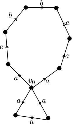
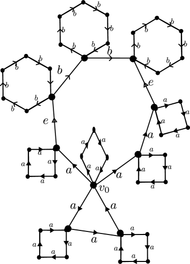
Figure 2: The $\mathcal{A}_{0}$ from the input $(aaa,aebbe^{-1}a^{-1}a^{-1})$ and $\mathcal{A}_{1}$, the result of attaching a copy of the appropriate Cayley graph at every vertex of $\mathcal{A}_{0}$.

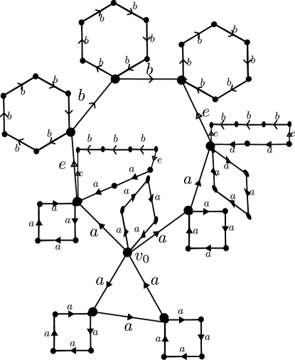
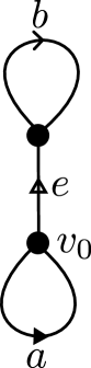
Figure 3: The graph $\mathcal{A}_{2}$ and the final folded graph $\mathcal{A}_{F}$, obtained by the standard folding algorithm.

In particular, from the graph $\mathcal{A}_{F}$, we see that, for example, the element given by the word $W=a^{2}eb^{3}e^{-1}a^{-1}$, as we can read this word as a loop starting and ending at $v_{0}$. In fact, we see that $H=\pi_{1}(\mathbb{A},u)$. In general, it may be that an unreduced word representing an element of the subgroup may not be readable in the final folded graph $\mathcal{A}_{F}$.

5 Proof of correctness

In this section, we show that the algorithm given in Section 4.1 produces an output with the desired properties. The argument we give is purely combinatorial, but it is guided by the following idea: if the Cayley graphs we attach during vertex saturation were actually Cayley 2-complexes (i.e. we add 2-cells so that they are simply connected and admit a free action by the $\mathbb{A}_{v}$) and if the loops we add during edge saturation actually bounded 2-cells, then any path in $\mathcal{A}_{F}$ can be homotoped to a path with reduced label.

Convention 5.1.

For this section, we will fix $\pi_{1}(\mathbb{A},v)$, a tuple $(W_{1},\ldots,W_{n})$ of input words, as well as the subgroup $H\leq\pi_{1}(\mathbb{A},v)$.

Proposition 5.2.

Let $\mathcal{A}_{F}$ be the $\mathbb{A}$-graph produced by the algorithm in Section 4.1, and let $v_{0}$ be its basepoint. Let $(W_{1},\ldots,W_{n})$ be the tuple of input words. Then we have an equality of subgroups

$$\pi_{1}(\mathcal{A}_{F},v_{0})=\langle\epsilon(W_{1}),\ldots,\epsilon(W_{n})\rangle=H\leq\pi_{1}(\mathbb{A},v).$$

Proof.

Let $\mathcal{A}_{0}$ be the graph (the bouquet of generators) formed at step 1 of the algorithm. Then it is clear that any element of $\pi_{1}(\mathcal{A}_{0},v_{0})$is equal to the long product of the elements in $\{\epsilon(W_{1}),\ldots,\epsilon(W_{n})\}^{\pm 1}=H$. Our goal is to show that this equality is preserved throughout the folding algorithm.

Vertex saturation. Step 2 involves attaching copies of Cayley graphs of vertex groups at various vertices of $\mathcal{A}_{0}$. We will consider the effect of attaching a single one of these Cayley graphs. Let $\mathcal{A}$ be an $\mathbb{A}$-graph, let $u\in{\mathbf{Verts}\left(\mathcal{A}\right)}$, let $[u]\in{\mathbf{Verts}\left(A\right)}$ be its label, and consider the $\mathbb{A}$-graph $\mathcal{A}^{\prime}$ obtained as the quotient of the union

$$\mathcal{A}\cup(\Gamma_{[u]},u^{\prime})/u\sim u^{\prime},$$

where $\Gamma_{[u]}$ is a copy of the given Cayley graph of $\mathbb{A}_{[}u]$ and $u^{\prime}$ is some vertex of the Cayley graph. Let $\rho$ be a loop based at $v_{0}$ in $\mathcal{A}^{\prime}$. Then we can express $\rho$ as a concatenation

$$\rho_{1}*\gamma_{1}*\cdots*\gamma_{n}*\rho_{n},$$

where the $\gamma_{i}$ are maximal subpaths that lie in $\Gamma_{[u]}.$ By maximality, the $\gamma_{i}$ must all be loops based at $u$, the vertex that is identified with the vertex $u^{\prime}$. Now, the $\rho_{i}$ may not be loops, but their evaluations $\epsilon(\rho_{i})$ are well-defined elements of $\mathbf{Bass}(\mathbb{A})$ and the product $\epsilon(\rho_{1})\epsilon(\gamma_{1})\cdots\epsilon(\gamma_{n})\epsilon(\rho_{n})\in\pi_{1}(\mathbb{A},v)\leq\mathbf{Bass}(\mathbb{A})$. For any loop $\ell$ in $\Gamma_{[u]}$, we must have that $\epsilon(\ell)\in\mathbb{A}_{[u]}$ and that $\epsilon(\ell)=1$. It follows that

$$\epsilon(\rho_{1}*\gamma_{1}*\cdots*\gamma_{n}*\rho_{n})=\epsilon(\rho_{1})\cdots\epsilon(\rho_{n}),$$

and since all the $\gamma_{i}$ are loops, the concatenation $\rho^{\prime}=\rho_{1}*\cdots*\rho_{n}$ is well defined.

Since there is an inclusion $\mathcal{A}\subset\mathcal{A}^{\prime}$, we have $\pi_{1}(\mathcal{A},v_{0})\leq\pi_{1}(\mathcal{A}^{\prime},v_{0})$. We have just shown that for any $g\in\pi_{1}(\mathcal{A}^{\prime},v_{0})$ represented by a loop $\rho^{\prime}$ in $\mathcal{A}^{\prime}$ based at $v_{0}$, there is a loop $\rho$ in $\mathcal{A}$ based at $v_{0}$ such that $\epsilon(\rho^{\prime})=\epsilon(\rho)=g$. Thus $\pi_{1}(\mathcal{A}^{\prime},v_{0})\leq\pi_{1}(\mathcal{A},v_{0})$. Since vertex saturation involves performing this operation repeatedly, it follows that $\pi_{1}(\mathcal{A}_{1},v_{0})=\pi_{1}(\mathcal{A}_{0},v_{0})=H$.

Edge saturation. Step 3 involves attaching loops $\ell_{r}$, whose labels $\mu(r)$ are precisely relations in $R$, so that $\epsilon(\ell_{r})=1$. An argument that is almost identical to the vertex saturation case establishes $\pi_{1}(\mathcal{A}_{2},v_{0})=\pi_{1}(\mathcal{A}_{1},v_{0})=H$.

Folding. Step 4 of the algorithm involves classical Stallings foldings. Our notation was chosen to match that of [KM02]. By applying [KM02, Lemma 3.4] repeatedly we have $\overline{L(\mathcal{A}_{2},v_{0})}=\overline{L(\mathcal{A}_{F},v_{0})}$, thus

$$\pi_{1}(\mathcal{A}_{F},v_{0})=\epsilon(\overline{L(\mathcal{A}_{F},v_{0})})=\epsilon(\overline{L(\mathcal{A}_{2},v_{0})})=\pi_{1}(\mathcal{A}_{2},v_{0})=H,$$

as required. ∎

The main difficulty when dealing with graphs of groups is that there are multiple equally valid ways to represent an element as a word. One way to overcome this is to introduce normal forms. In this paper, we chose instead to show that $L(\mathcal{A}_{F},v_{0})$ contains all possible reduced forms of elements.

Convention 5.3.

When $\epsilon_{i}$s occur as exponents, they are either $1$ or $-1$.

A first crucial observation is that in a fully folded directed $X$-labelled graph, a path $\rho$ is reduced if and only if its label $\mu(\rho)$ is a freely reduced word in $(X^{\pm 1})^{*}$. Consider the folded graph $\mathcal{A}_{F}$, and for a given $v\in{\mathbf{Verts}\left(A\right)}$, consider the subgraph consisting of all edges with labels in $\mathscr{G}_{v}$. We call the connected components of this subgraph the $v$-components of $\mathcal{A}_{F}$. It is clear that each vertex of $\mathcal{A}_{F}$ lies in some $v$ component, and that deleting all edges with a label in ${\mathbf{Edges}\left(A\right)}$ will disconnect $\mathcal{A}_{F}$ into various $v$-components.

It follows that given a path $\rho$ in $\mathcal{A}_{F}$, we have an $\mathbb{A}$-decomposition

$$\rho=\alpha_{1}*e_{1}^{\epsilon_{1}}*\cdots e_{n}^{\epsilon_{n}}*\alpha_{n}$$

which is the unique decomposition with the $\alpha_{i}$ being maximal subpaths contained in $v$-components for an appropriate $v\in{\mathbf{Verts}\left(A\right)}$, and where the $e_{j}$s have label $\mu(e_{j})\in{\mathbf{Edges}\left(A\right)}$. The paths $\alpha_{i}$s are called ${\mathbf{Verts}\left(A\right)}$-components. We now give our two substitution lemmas.

Lemma 5.4.

Let $\rho=\alpha_{1}*e_{1}^{\epsilon_{1}}*\cdots*\alpha_{i}*\cdots*e_{n}^{\epsilon_{n}}\alpha_{n_{1}}$ be the $\mathbb{A}$-splitting of a path in $\mathcal{A}_{F}$. Let $\alpha_{i}$ lie in a $v$-component, and let $W_{i}^{\prime}\in(\mathscr{G}_{v}^{\pm 1})^{*}$ be a word such that $\epsilon(\alpha_{i})=_{\mathbb{A}_{v}}\epsilon(W_{i}^{\prime})$. Then there is a path $\alpha_{i}^{\prime}$ with the same endpoints as $\alpha_{i}$ such that $\mu(\alpha_{i}^{\prime})=W_{i}^{\prime}$ and

$$\rho^{\prime}=\alpha_{1}*e_{1}^{\epsilon_{1}}*\cdots*\alpha_{i}^{\prime}*\cdots*e_{n}^{\epsilon_{n}}\alpha_{n}$$

is also a path in $\mathcal{A}_{F}$ with the same endpoints as $\rho$. Furthermore $\epsilon(\rho)=\epsilon(\rho^{\prime})$.

Proof.

Let $v_{i}\in{\mathbf{Verts}\left(\mathcal{A}_{F}\right)}$ be the initial vertex of $\alpha_{i}$, and set $v=[v_{i}]$. The preimages of $v_{i}$ in $\mathcal{A}_{2}$ are either as vertices in the bouquet of generators in step 1, vertices in one of the copies of Cayley graphs of $\mathbb{A}_{v}$ added in step 2, or vertices in one of the loops added in step 3. In all cases, when performing the folding process, any preimage of $v_{i}$ is eventually identified with the vertex of some Cayley graph added in step 2. So we take a preimage $\hat{v}_{i}$ of $v_{i}$ that lies in some copy $\Gamma^{\prime}_{v}$ of a Cayley graph of $\mathbb{A}_{v}$.

By properties of the Cayley graph, since $\mu(\alpha_{i})=_{\mathbb{A}_{v}}\mu(\alpha_{i}^{\prime})$, there exist paths $\hat{\alpha}_{i}$ and $\hat{\alpha}_{i}^{\prime}$ with labels $\mu(\alpha_{i})$ and $\mu(\alpha_{i}^{\prime})$ respectively both originating at $\hat{v}_{i}$ and terminating at the same vertex $\hat{u}_{i}$. Because $\mathcal{A}_{2}\to\mathcal{A}_{F}$ is realized by a continuous map, $\hat{\alpha}_{i}$ is mapped to a path in $\mathcal{A}_{F}$ starting at $v_{i}$, and because in a folded graph there is at most one path originating from a vertex with a given label, we have that $\hat{\alpha}_{i}$ is mapped to $\alpha_{i}$. It follows that $\alpha_{i}^{\prime}$, the image of $\hat{\alpha}_{i}^{\prime}$, has the same endpoints as $\alpha_{i}$, so $\rho^{\prime}$ is also a path in $\mathcal{A}_{F}$ with the same endpoints.

Finally, the equality $\epsilon(\rho)=\epsilon(\rho^{\prime})$ follows from the $\mathbf{Bass}(\mathbb{A})$-equality

$$\epsilon(\rho^{\prime})=\epsilon(\alpha_{1})\epsilon(e_{1})^{\epsilon_{1}}\cdots\epsilon(\alpha_{i}^{\prime})\cdots\epsilon(e_{n})^{\epsilon_{n}}\epsilon(\alpha_{n_{1}}),$$

and the fact that $\epsilon(\alpha_{i}^{\prime})=\epsilon(\alpha_{i}).$ ∎

Lemma 5.5.

Let $\rho=\alpha_{1}*{e_{1}}^{\epsilon_{1}}*\cdots\alpha_{i}*{e_{i}}^{\epsilon_{i}}*\alpha_{i+1}*\cdots*{e_{n}}^{\epsilon_{n}}\alpha_{n_{1}}$ be the $\mathbb{A}$-splitting of a path in $\mathcal{A}_{F}$, and let $\mu(e_{i})W(t_{\mu(e_{i})}(h))\mu(e_{i})^{-1}V(i_{\mu(e_{i}}(h))^{-1}$ be one of the relations in (5). Then the 1-edged path $e_{i}^{\epsilon_{i}}$ can be replaced by a path

$$\begin{cases}\nu*(e_{i}^{\prime})^{\epsilon_{i}}*\omega&\textrm{ if $\epsilon_{i}=1$}\\ \omega*(e_{i}^{\prime})^{\epsilon_{i}}*\nu&\textrm{ if $\epsilon_{i}=-1$}\\ \end{cases}$$

where $\mu(e_{i})=\mu(e_{i}^{\prime})$ and $\mu(\omega)=W(t_{\mu(e_{i})}(h))^{-1}$ and $\mu(\nu)=V(i_{\mu(e_{i})}(h))$, giving a new path

$$\rho^{\prime} = \alpha_{1}*{e_{1}}^{\epsilon_{1}}*\cdots*\alpha_{i}*\omega^{-1}*e_{i}^{\prime}*\nu*\alpha_{i+1}*\cdots*{e_{n}}^{\epsilon_{n}}\alpha_{n_{1}}$$

or

$$\rho^{\prime} = \alpha_{1}*{e_{1}}^{\epsilon_{1}}*\cdots*\alpha_{i}*\nu*(e_{i}^{\prime})^{-1}*\omega^{-1}*\alpha_{i+1}*\cdots*{e_{n}}^{\epsilon_{n}}\alpha_{n_{1}}$$

that is also in $\mathcal{A}_{F}$ with the same endpoints and $\epsilon(\rho)=\epsilon(\rho^{\prime})$.

Proof.

Take a preimage $\hat{e}_{i}$ of $e_{i}$ in $\mathcal{A}_{2}$. $\hat{e}_{i}$ was either added in step 1 or in step 3. We will suppose that $\hat{e}_{i}$ was added in step 3, and we will assume $\epsilon_{i}=1$. The other case follows from a similar argument.

In this case, $\hat{e}_{i}$ is added as part of a loop $\ell_{r}$ with

$$\mu(\ell_{r})=\mu(e_{i})W(t_{\mu(e_{i})}(h_{i}))\mu(e_{i})^{-1}V(i_{\mu(e_{i})}(h_{i}))^{-1}$$

as shown in Figure 4.

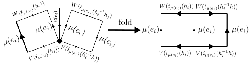
Figure 4: The two squares represent loops added in step 3. The bold edge on the left is the preimage $\hat{e}_{i}$ of $e_{i}$ with label $\mu(e_{i})$, and the bold path on the right is the new path $\hat{\nu}*\hat{e}_{i}^{\prime}*\hat{\omega}$. The decorations are either edge or path labels.

An important feature of the folding algorithm is that the order in which we perform folds does not affect the final result. By step 3 of the algorithm, there will be another loop with label $\mu(e_{i})W(t_{\mu(e_{i})}(h_{i}^{-1}h))\mu(e_{i})^{-1}V(i_{\mu(e_{i})}(h_{i}^{-1}h))^{-1}$ attached to a corner of $\ell_{r}$ as shown in Figure 4, and we can immediately fold the three edges labelled $\mu(e_{i})$ as shown in Figure 4 in order to obtain an intermediate graph $\mathcal{A}^{\prime}$ such that there is a sequence of continuous maps $\mathcal{A}_{2}\twoheadrightarrow\mathcal{A}^{\prime}\twoheadrightarrow\mathcal{A}_{F}$.

In $\mathcal{A}^{\prime}$, looking again at Figure 4, we see that there is a path $\hat{\nu}*\hat{e}_{i}^{\prime}*\hat{\omega}$ with the same endpoints as $\hat{e}_{i}$ where

$$\mu(\hat{\nu}) = V(i_{\mu(e_{i})}(h_{i}))^{-1}V(i_{\mu(e_{i})}(h_{i}^{-1}h))$$

$$\mu(\hat{e}_{i}^{\prime}) = \mu(e_{i})$$

$$\mu(\hat{\omega}) = W(t_{\mu(e_{i})}(h_{i}^{-1}h))^{-1}W(t_{\mu(e_{i})}(h_{i}))$$

This path descends to a concatenation of path $\nu^{\prime}*e_{i}^{\prime}*\omega^{\prime}$ with the same endpoints as $e_{i}$. Noting that in the respective vertex groups we have

$$\mu(\nu^{\prime})=V(i_{\mu(e_{i})}(h_{i}))^{-1}V(i_{\mu(e_{i})}(h_{i}^{-1}h))=V(i_{\mu(e_{i})}(h))$$

and

$$\mu(\omega^{\prime})=W(t_{\mu(e_{i})}(h_{i}^{-1}h))^{-1}W(t_{\mu(e_{i})}(h_{i}))=W(t_{\mu(e_{i})}(h))^{-1}$$

we see that we can now apply Lemma 5.4 (applied to paths consisting of a single $\mathbb{A}$-component) to obtain paths $\nu$ and $\omega$ as desired and the result follows.

∎

Lemma 5.6.

Let $\rho$ be a path in $\mathcal{A}_{F}$ and suppose the label $\mu(\rho)\in(X^{\pm 1})^{*}$ is not freely reduced. Then there is another path $\rho^{\prime}$ with the same endpoints as $\rho$ with $\epsilon(\rho^{\prime})=\epsilon(\rho)$, but with $\mu(\rho^{\prime})$ freely reduced.

Proof.

If $\mu(\rho)$ is already freely reduced, there is nothing to show. Suppose $\mu(\rho)$ is not freely reduced. Then $\mu=Lx^{\pm 1}x^{\mp 1}R$ for words $L,R\in(X^{\pm 1})^{*}$ and some $x\in X$, and it follows that $\rho=\lambda*e_{i}^{\epsilon_{i}}*e_{i+1}^{\epsilon_{i+1}}*\sigma$ where $\mu(e_{i})=\mu(e_{i+1})=x$.

Because $\mathcal{A}_{F}$ is folded, $e_{i}=e_{i+1}$ and $\epsilon_{i}=-\epsilon_{i+1}$, so $\rho^{\prime}=\lambda*\sigma$ is a well-defined concatenation in $\mathcal{A}_{F}$ with $\mu(\rho^{\prime})$ freely equivalent to $\mu(\rho)$. Since $\rho^{\prime}$ is shorter than $\rho$, we can repeat the process until we get the desired result. ∎

Proposition 5.7.

$g\in H\leq\pi_{1}(\mathbb{A},v)$ if and only if for any reduced word $W\in(X^{\pm 1})^{*}$ with $\epsilon(W)=g$, there is a loop $\ell_{W}$ based at $v_{0}$ in $\mathcal{A}_{F}$ such that $\mu(\ell_{w})=W.$

Proof.

A Van Kampen diagram for a group presentation $\langle X|R\rangle$ is a simply connected CW 2-complex $D$ equipped with a fixed embedding in the plane. The 1-skeleton $D^{(1)}$ of $D$ has the structure of a directed $X$-labelled graph. We can read off words in $R^{\pm 1}$ along the boundaries of the 2-cells in $D$. By Van Kampen’s Lemma, see [LS01, §V.1], for any word $W$ representing the identity in $\langle X|R\rangle$, there is a Van Kampen diagram $D$ with a vertex $d_{0}$ on its boundary such that the word $W$ can be read along the path that traces the boundary of $D$ when read in the clockwise direction.

Let $g\in H$ be arbitrary, and let $W$ be a reduced word with $\epsilon(W)=g$ (this is to say that $W$ is freely reduced and has minimal syllable length among all possible words representing $g$). By Proposition 5.2, there is some loop $\ell$ in $\mathcal{A}_{F}$ based at $v_{0}$ such that $\epsilon(\ell)=g$. Let $\mu(\ell)=W^{\prime}$. It follows that $W^{\prime}W^{-1}$ represents the identity in $\langle X|R\rangle$ which is our presentation for $\mathbf{Bass}(\mathbb{A})$. Consider the Van Kampen diagram $D=D(W,W^{\prime})$ for $W^{\prime}W^{-1}$. It has two vertices $d_{l},d_{r}$ (a “leftmost” and a “rightmost”) such that for the path $\rho^{\prime}$ that travels in $\partial D$ from $d_{l}$ to $d_{r}$ in the clockwise direction along the top of $D$, we have $\mu(\rho^{\prime})=W^{\prime}$ and for the path $\rho$ that travels in $\partial D$ from $d_{l}$ to $d_{r}$ in the counter-clockwise direction along the bottom of $D$ we have $\mu(\rho)=W$. This is depicted in Figure 5.

Figure 5: The Van Kampen diagram $D(W,W^{\prime})$ for a pair of words representing the same group element. Note that this diagram has three degree 1 vertices, one of which is $d_{l}$.

We know that $W^{\prime}$ is the label of some loop in $\mathcal{A}_{F}$ based at $v_{0}$. We want to show $W$ can also be read off some loop in $\mathcal{A}_{F}$ based at $v_{0}$. We will do this by deleting cells from $D$ in such a way that the cells in the bottom path $\rho$ never get deleted but such that the new top paths still have labels in $L(\mathcal{A}_{F},v_{0})$. The number of cells in $D$ can be thought of as a measure of how different $W$ is from $W^{\prime}$, and the process will terminate in a (degenerate) Van Kampen diagram consisting only of $\rho$. The result will follow.

Suppose we have a Van Kampen diagram $D(W^{\prime},W)$ with $W$ reduced. An elementary deletion will be one of the following operations:

1. Remove a spur $w$. If there is a vertex $w$ of degree 1 other than $d_{l}$ or $d_{r}$, delete $w$ and the unique edge adjacent to $w$.

2. Remove a free face $e$ with label in ${\mathbf{Edges}\left(A\right)}$. If there is an edge $e\in\partial D$ that is in the boundary of some 2-cell $C$ with label in ${\mathbf{Edges}\left(A\right)}$, then delete $e$ and the interior of $C$.

3. Remove a free face $e$ with label in $\mathscr{G}_{v}$ for some $v\in{\mathbf{Verts}\left(A\right)}$. If there is an edge $e\in\partial D$ that is in the boundary of some 2-cell $C$ coming from a relation of $\mathbb{A}_{[v]}$, then delete $e$ and the interior of $C$.

The presence of a spur implies that the word read around $\partial D$ is not freely reduced. Since $W$ is reduced, the spur cannot be covered by the path $\rho$. It follows that if there is a spur other than $d_{l}$ or $d_{r}$, $\mu(\rho^{\prime})$ is not freely reduced. By successively removing spurs and taking new “top” boundary paths, we arrive at $\rho^{\prime\prime}$ such that $\mu(\rho^{\prime\prime})$ is the free reduction of $\mu(\rho^{\prime})$. By Lemma 5.6 there is a loop $\hat{\rho}^{\prime\prime}$ in $\mathcal{A}_{F}$ based at $v_{0}$ with label $\mu(\rho^{\prime\prime})$.

If we perform either of the elementary deletions (b) or (c), we get a new Van Kampen diagram $D^{\prime}$ which can be seen as a sub-diagram of $D$. Because of that, doing this also comes with an embedding in the plane and a well-defined boundary word. This is depicted in Figure 6.

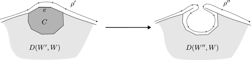
Figure 6: The new top boundary path $\rho^{\prime\prime}$ after applying elementary deletion (b) or (c).

By Lemma 5.5 or Lemma 5.4 (respectively), if the deleted edge $e$ lies in the path $\rho^{\prime}$, then there is a closed loop in $\mathcal{A}_{F}$ based at $v_{0}$ with label $\mu(\rho^{\prime\prime})=W^{\prime\prime}$. We therefore proceed as follows:

1. Start with $D=D(W^{\prime},W)$.

2. Do the first possible applicable elementary deletion below:

   1. If there is a spur besides $d_{l}$ or $d_{r}$, which will never lie in the bottom path $\rho$, remove it.

   2. If there is an edge $e$ with label in ${\mathbf{Edges}\left(A\right)}$ that lies in $\rho^{\prime}$ but not in $\rho$, delete it and the 2-cell $C$ that contains it using the elementary deletion (b).

   3. If there is an edge $e$ with label in $\mathscr{G}_{v}$ for an appropriate $v$ that lies in $\rho^{\prime}$ but not in $\rho$, and $e$ is contained in a 2-cell $C$ coming from a relation in $\mathbb{A}_{v}$, delete it and the 2-cell that contains it using the elementary deletion (c).

3. If this gives a new diagram $D(W^{\prime\prime},W)\subset D(W^{\prime},W)\subset\mathbb{R}^{2}$ with a new top boundary path $\rho^{\prime\prime}$, go back to step 2 and repeat the process. Otherwise, terminate.

If this process terminates after $n$ steps with a diagram without any 2-cells, then the diagram must be a tree with spurs $d_{l}$ and $d_{v}$, which means that $\rho^{(n+1)}=\rho$, and by Lemmas 5.4, 5.5, and 5.6 we have that $\mu(\rho^{(n+1)}=W$ is the label of a closed loop in $\mathcal{A}_{F}$ based at $v_{0}$ as required.

Suppose now that this process terminates but there are remaining 2-cells. We distinguish two cases.

Case 1: One of the remaining 2-cells comes from a relation involving a symbol from ${\mathbf{Edges}\left(A\right)}$. We will argue that this situation is impossible. Recalling the set of relations $R$ given in (5), we see that any such 2-cell $C$ has exactly one pair of edges with label in $e\in{\mathbf{Edges}\left(A\right)}$ that we think of as the top and bottom of the 2-cell. The other two paths forming $\partial C$ consist of edges with labels in $\mathscr{G}_{i(e)}$ and $\mathscr{G}_{t(e)}$. Such 2-cells combine to form $e$-strips as depicted in Figure 7.

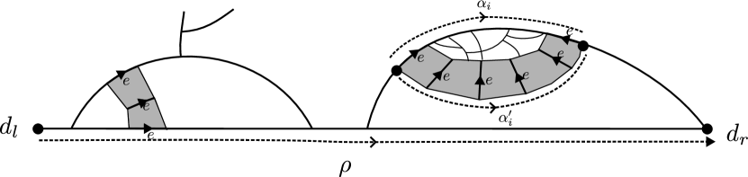
Figure 7: Two $e$-strips.

An $e$-strip $\mathcal{S}\subset D$ is innermost if one of the components of $D\setminus\mathcal{S}$ contains no $e^{\prime}$-strips for any $e^{\prime}\in{\mathbf{Edges}\left(A\right)}$.

Claim: If $\mu(\rho)$ is reduced in the sense of Definition 3.2, then there are no $e$-strips whose extremities both lie in $\rho$. Indeed, if such an $e$-strip existed, then there would be an innermost such strip. Looking at Figure 7, we see that if this happens, $\rho$ would have a subpath $\alpha_{i}$ such that there exists another path $\alpha_{i}^{\prime}$ with the same endpoints. The union of these paths encloses a van Kampen (sub) diagram so $\epsilon(\alpha_{i})=\epsilon(\alpha_{i}^{\prime}$), but where the edges in $\alpha_{i}^{\prime}$ only have labels in $\mathscr{G}_{i(e)}$ or $\mathscr{G}_{t(e)}$. It follows that if we take the paths $\rho=\alpha*\alpha_{i}*\beta$ and $\rho^{\flat}=\alpha*\alpha_{i}^{\prime}*\beta$ in $D$, we get $\epsilon(\rho)=\epsilon(\rho^{\flat})$, but $\mu(\rho^{\flat})$ contains fewer symbols from ${\mathbf{Edges}\left(A\right)}$, thus smaller syllable length, than $\mu(\rho)$, which by Lemma 3.3 contradicts that $\mu(\rho)=W$ is a reduced word representing $\epsilon(\rho)$. This proves the claim.

Now, if the algorithm terminated in Case 1, then this means that every edge in $\rho^{(n+1)}$ is either not contained in a 2-cell, or it is an edge with label in $\mathscr{G}_{v}$ for some $v\in{\mathbf{Verts}\left(A\right)}$ that is contained in some 2-cell coming from a relation involving a pair of symbols in $e\in{\mathbf{Edges}\left(A\right)}$, i.e. lying in the ”side” of an $e$-strip. Such 2-cells assemble into $e$-strips, and in this case, the extremities of all $e$-strips must lie in $\rho$, which contradicts the claim above. It follows that Case 1 cannot occur.

Case 2: All remaining 2-cells come from the relations in the $\mathbb{A}_{v},v\in{\mathbf{Verts}\left(A\right)}$. In this case, since none of the edges of $\rho^{(n+1)}$ lie in any 2-cells, we must be in a situation as depicted in Figure 8.

Figure 8: When none of the edges of $\rho^{(n+1)}$ lie in the boundary of a 2-cell.

A first consequence of Case 2 is that all edges with labels in ${\mathbf{Edges}\left(A\right)}$ must lie in the path $\rho^{(n+1)}$. Furthermore, since both $\mu(\rho)$ and $\mu(\rho^{(n+1)})$ represent elements in $\pi_{1}(\mathbb{A},v)$, deleting all edges with labels in ${\mathbf{Edges}\left(A\right)}$ separates $D$ in such a way that for every connected component, there is some $v\in{\mathbf{Verts}\left(A\right)}$ such that all edges in that component have a label in $\mathscr{G}_{v}$. These components also coincide with the ${\mathbf{Verts}\left(A\right)}$-components of $\rho^{(n+1)}$. Let $\alpha_{i}$ be a ${\mathbf{Verts}\left(A\right)}$-components of $\rho^{(n+1)}$, and consider the subpath $\alpha^{\prime}_{i}$ of $\rho$ depicted in Figure 9.

Figure 9: Subpaths of $\rho^{(n+1)}$ and $\rho$ in the same ${\mathbf{Verts}\left(A\right)}$-component with the same evaluations.

Seeing as $\alpha_{i},\alpha_{i}^{\prime}$ bound a van Kampen (sub) diagram, we have $\epsilon(\alpha_{i})=\epsilon(\alpha_{i}^{\prime})$, and by repeatedly applying Lemma 5.4, if $\mu(\rho^{(n+1)})=W^{(n+1)}$ is the label of a based loop in $\pi_{1}(\mathcal{A}_{F},v_{0})$, then so is $W=\mu(\rho)$.

Since Case 1 and Case 2 exhausted all remaining possibilities, the result follows.

∎

Proof of Theorem 1.2.

The result now follows from Proposition 5.7 and the running time analysis in Section 4.2. ∎

6 Applications

6.1 Reducing words

Given a word $W$ in $(X^{\pm 1})^{*}$, there is a naive algorithm to pass to a reduced form by reading through $W$ and making substitution $e^{\pm 1}he^{\mp 1}\mapsto h^{\prime}$, where $e\in{\mathbf{Edges}\left(A\right)}$ and where $e^{\pm 1}he^{\mp 1}=h^{\prime}$ is a relation of $\mathbf{Bass}(\mathbb{A})$, and then starting over until no more cancellable ${\mathbf{Edges}\left(A\right)}$-letters remain. This algorithm runs in quadratic time in the word length. We propose a faster algorithm.

Proposition 6.1.

Suppose that a graph of groups $\mathbb{A}$ is explicitly given as in Section 2.1 and such that for every vertex group, every element of the image of the incident edge group is assigned a symbol as a generator of that vertex group. Then there is an algorithm that takes as input a word $W\in(X^{\pm 1})^{*}$ representing an element of $\pi_{1}(\mathbb{A},v)$ and outputs a reduced word $\bar{W}$ (in the sense of Definition 3.2) such that $\epsilon(W)=\epsilon(\bar{W})$ which runs in time $O(n\log^{*}(n))$ where $n=|W|$.

Proof of Proposition 6.1.

We note that our requirement on the presentation ensures that all the relations in (5) have length 4. The algorithm is a slight variation of the folding algorithm. As we present the algorithm, we will provide analysis.

Start by constructing a based linear directed $X$-labelled graph $(\mathcal{W}_{0},v_{0})$ with endpoints $v_{0}$ and $u_{0}$ so that the unique reduced path $\rho_{0}$ from $v_{0}$ to $u_{0}$ has label $W$. We note that $\pi_{1}(\mathcal{W}_{0},v_{0})=\{1\}$. We now treat $(\mathcal{W}_{0},v_{0})$ exactly as the graph constructed in step 1 of the folding algorithm and proceed to perform the folding algorithm and arrive at a terminal based graph $(\mathcal{W}_{F},v_{0})$.

Following Section 5, we see that $\pi_{1}(\mathcal{W}_{F},v_{0})=\pi_{1}(\mathcal{W}_{0},v_{0})=\{1\}$. Recall that we have a continuous map $\mathcal{W}_{0}\to\mathcal{W}_{F}$. Following our notation convention, we denote the images $v_{0}$ and $u_{0}$ in $\mathcal{W}_{0}$ in $\mathcal{W}_{F}$ by the same symbols $v_{0}$ and $u_{0}$ respectively. Let $\rho$ be a shortest path in $\mathcal{W}_{F}$ from $v_{0}$ to $u_{0}$. We claim that the label $\mu(\rho)$ is reduced in the sense of Definition 3.2. Indeed, suppose that was not the case. Then $\rho=\rho_{1}*\beta*\rho_{2}$, where $\mu(\beta)=e^{\pm 1}U(\mathscr{G}_{v}^{\mp 1})e^{\pm 1}$ is cancellable. This means that $U(\mathscr{G}_{v}^{\pm 1})$ evaluates to an element in the image of an edge group, so by Lemma 5.4, we can replace $\beta$ with $\beta^{\prime}$ with the same endpoints and where $\mu(\beta^{\prime})=e^{\pm 1}a_{U}e^{\pm 1}$, with $a_{U}$ being a single letter representing an element of the incident edge group. Because of edge saturation and the argument of Lemma 5.5, we know that we can replace $\beta^{\prime}$ by $\beta^{\prime\prime}$, where $\beta^{\prime\prime}=b_{U}$, $e^{\pm 1}a_{U}e^{\pm 1}=b_{U}$ is an identity in $\mathbf{Bass}(\mathbb{A})$, and $b_{U}$ consists of a single letter. We note that $\rho^{\prime}=\rho_{1}*\beta^{\prime\prime}\rho_{2}$ is strictly shorter than $\rho$ but still joins $v_{0}$ to $u_{0}$, which is a contradiction. It follows that $\mu(\rho)$ must be reduced.

Let $\bar{\rho}_{0}$ be the image of the path $\rho_{0}$ in $\mathcal{W}_{0}$ in $\mathcal{W}_{F}$. Then $\bar{\rho}_{0}$ also joins $v_{0}$ to $u_{0}$, so $\mu(\bar{\rho}_{0}*\rho^{-1})\in\pi_{1}(\mathcal{W}_{F},v_{0})=\{1\}$. Therefore $\epsilon(\rho_{0})=\epsilon(\rho)$, and $\mu(\rho)$ is the desired reduced form.

We finally note that $\rho$ can be found from $\mathcal{W}_{F}$ by performing a depth-first search rooted at $v_{0}$ and directing the tree so that descendants point to ancestors. Once $u_{0}$ is found the path $\rho^{-1}$ can be computed in time linear in the size of the tree by tracing the unique directed path back to the root. Noting that the degree of the vertices in $\mathcal{W}_{F}$ is uniformly bounded by a constant that depends on our presentation, we see that this can be achieved in time $O(m\log^{*}(m))$, where $m$ is the total number of vertices and edges of $\mathcal{W}_{0}$. ∎

6.2 Detecting freeness and equality of subgroups

This next result is easy to show using Bass-Serre theory.

Proposition 6.2.

$H\leq\pi_{1}(\mathbb{A},v_{0})$ is a free group if and only if every ${\mathbf{Verts}\left(A\right)}$-component $W$ is isomorphic to a copy of the Cayley graph $\Gamma_{[w]}$, where $w\in{\mathbf{Verts}\left(W\right)}$.

Proof.

An element $g\in\pi_{1}(\mathbb{A},v)$ fixes a point in the dual Bass-Serre tree if and only if it is conjugate to one of the vertex groups $\mathbb{A}_{v}$ for some $v\in{\mathbf{Verts}\left(A\right)}$. Thus, $H$ contains such an element if and only if there is a loop in $(\mathcal{A}_{H},v_{0})$ with reduced label $WfW^{-1}$, where $f\in\mathbb{A}_{v}\setminus\{1\}$. It follows that if $\rho$ is a path in $(\mathbb{A},v)$ starting at $v$ with label $W$, then there must be a loop at the endpoint of $\rho$ with label $f$. Thus $WfW^{-1}$ is non-trivial if and only if $f\neq 1$, and such an element exists if and only if some ${\mathbf{Verts}\left(A\right)}$-component of $\mathcal{A}_{H}$ is not a Cayley graph of a vertex group, but rather a proper quotient of such a Cayley graph so that it contains a loop with a label that doesn’t evaluate to the identity.

Since $\mathbb{A}$ is a graph of finite groups, if some $g\in H$ fixes a vertex in the Bass-Serre tree, then that element has finite order and $H$ is not free. If there are no such elements, then $H$ acts freely on $T$ and therefore is free. ∎

An immediate application of the Theorem 1.2 and Proposition 6.1 is:

Proposition 6.3.

Let $(K_{1},\ldots,K_{r})$ and $(W_{1},\ldots,W_{s})$ be two tuples of words in $X$. Then there is an algorithm that runs in time $O(n\log^{*}(n))$, where $n$ is the total length of all the words in the input and determines whether the subgroups $\left\langle{K_{1},\ldots,K_{r}}\right\rangle$ and $\left\langle{W_{1},\ldots,W_{s}}\right\rangle$ are equal.

Proof.

Using Proposition 6.1 in time $O(n\log^{*}(n))$, we can replace all the $K_{i},W_{j}$ by reduced forms. We now perform the folding algorithm, again in time $O(n\log^{*}(n))$, and then verify if $K_{i}\in\left\langle{W_{1},\ldots,W_{s}}\right\rangle$ and $W_{j}\in\left\langle{K_{1},\ldots,K_{r}}\right\rangle$ for all $K_{i},W_{j}$. This takes time $O(n)$ once the folded graphs are constructed and establishes whether or not both inclusions

$$\left\langle{K_{1},\ldots,K_{r}}\right\rangle\leq\left\langle{W_{1},\ldots,W_{s}}\right\rangle\textrm{~{}and~{}}\left\langle{W_{1},\ldots,W_{s}}\right\rangle\leq\left\langle{K_{1},\ldots,K_{r}}\right\rangle$$

hold. ∎

6.3 The proof of Theorem 1.1

We have that $\mathrm{GL}\left(2,\mathbb{Z}\right)\approx D_{6}*_{D_{2}}*D_{4}$, which we can express as a graph of groups where the underlying graph $A$ has vertices $u,v$ and a single edge $e$, with $i(e)=u$ and $t(e)=v$. We take $\mathbb{A}_{u}\approx D_{6}$ and $\mathbb{A}_{v}\approx D_{4}$. Now, following [DD89, $\S$I.5], we find $A=\begin{pmatrix}1&-1\\ 0&-1\end{pmatrix}\in D_{6},B=\begin{pmatrix}1&0\\ 0&-1\end{pmatrix}\in D_{4}$, and $C=\begin{pmatrix}0&1\\ 1&0\end{pmatrix}\in D_{6}\cap D_{4}=D_{2}$. Expressing these as elements of $\pi_{1}(\mathbb{A},v)$, we write $A=a\in\mathbb{A}_{u}$, $B=ebe^{-1},b\in\mathbb{A}_{v}$ and $C=c=ec^{\prime}e^{-1}$ where $c\in\mathbb{A}_{u}$ and $c^{\prime}\in\mathbb{A}_{v}$. Just as in Section 2.2, we can find a presentation $\mathbf{Bass}(\mathbb{A})=\langle X|R\rangle$ satisfying the requirements of Section 2.1 where $a\in\mathscr{G}_{u}\subset X\supset\mathscr{G}_{v}\ni b$.

Lemma 6.4.

Let

$$M=\begin{pmatrix}a&b\\ c&d\end{pmatrix}\in\mathrm{GL}\left(2,\mathbb{Z}\right)$$

and let $\mathrm{GL}\left(2,\mathbb{Z}\right)=\pi_{1}(\mathbb{A},u)$ where $\mathbb{A}$ is as given above and conforms to the requirements set out in Section 2.1. Fix the presentation, including a generating set, $\mathbf{Bass}(\mathbb{A})=\langle X|R\rangle$. Then $M$ can be represented as a word of length $O(|a|+|b|+|c|+|d|)$ in $(X^{\pm 1})^{*}$

Proof.

We can set $BA=E=\begin{pmatrix}1&-1\\ 0&1\end{pmatrix}$, and take the inverse $E^{-1}=\begin{pmatrix}1&1\\ 0&1\end{pmatrix}$. As elements of $\pi_{1}(\mathbb{A},u)$, we would then write

$$E=ebe^{-1}a,E^{-1}=a^{-1}eb^{-1}e^{-1},$$

where $a,b$ are defined as before.

Multiplying $M$ by $E^{\pm 1}$ on the left will correspond to adding or subtracting the second row from the first, and multiplying $M$ by $C$ on the left will correspond to swapping the rows of $M$. Thus these are sufficient to implement row reduction. We now row-reduce $M$ to the identity matrix.

The first objective is to use the Euclidean algorithm to find some matrix $N_{1}$ such that:

$$N_{1}\begin{pmatrix}a&b\\ c&d\end{pmatrix}=\begin{pmatrix}\gcd(a,c)&n\\ 0&u\end{pmatrix},$$

for some $n,u$. Up to multiplying on the left by some product length at most 3 of $B,C,-I_{2}$, we can assume that $0<a<c$ and both $a,c\geq 0$. By the division algorithm, there is $0\leq r<a$ such that $c=aq+r$. Take $F=CEC=\begin{pmatrix}1&0\\ -1&1\end{pmatrix}.$ We have

$$F^{q}M=\begin{pmatrix}a&b\\ c-qa&d-qb\end{pmatrix}=\begin{pmatrix}a&b\\ r&d^{\prime}\end{pmatrix}.$$

We now consider the absolute values of the entries of the resulting matrix. The entries $a$ and $b$ will be unchanged in $F^{q}M$, and by hypothesis, $0\leq c-qa<a\leq c$. Furthermore, we have that $c-r=qa\geq q$. Thus the sum of the entries in the first column decreased by at least $q$ after multiplication by $F^{q}$.

We now look at the second column. It suffices to compare $|d|$ to $|d^{\prime}|$. On the one hand, we have

$$ad-bc=\pm 1\textrm{~{}and~{}}ad^{\prime}-br=\pm 1,$$

since $\det(F^{q}M)=1$. This gives $|d^{\prime}|\leq 1+\left|\frac{br}{a}\right|$ and $|\frac{bc}{a}|-1\leq|d|$, and since $|c|\geq|r|$ (with equality only if $c=r=0$), we have that $|d^{\prime}|\leq|d|+2$. So the sum of the entries in the second column increased by at most 2.

To continue the Euclidean Algorithm, we would multiply by $C$ on the left to interchange the rows and repeat the process until we get the desired matrix

$$N_{1}=F^{q_{s}}C\cdots CF^{q_{1}}.$$

Repeating the argument given above we see that in passing from $M$ to $N_{1}M$ the sum of the entries in the first column decreased by at least $q_{1}+\cdots+q_{r}$ thus we have

$$s\leq\sum_{i=1}^{s}q_{i}\leq a+c$$

and it follows that $N_{1}$ can be represented by a word in $(X^{\pm 1})^{*}$ of length $O(a+c)$. We now have

$$N_{1}M=\begin{pmatrix}\gcd(a,c)&n\\ 0&u\end{pmatrix}\in\mathrm{GL}\left(2,\mathbb{Z}\right),$$

thus $\gcd(a,c),u\in\{-1,1\}$. As for the top right entry $n$, note that by repeating the argument above, we see that the entries in the second column increased by at most $2s\leq 2|a|+2|c|$ which easily gives

$$n\leq\max\{|b|,|d|\}+2|a|+2|c|\leq 2(|a|+|b|+|c|+|d|)$$

so, after perhaps multiplying by $B$ to make the bottom right entry positive, we have

$$E^{n}\begin{pmatrix}\pm 1&n\\ 0&1\end{pmatrix}=\begin{pmatrix}\pm 1&0\\ 0&1\end{pmatrix}\in D_{4}.$$ (8)

It follows that a matrix $M=\begin{pmatrix}a&b\\ c&d\end{pmatrix}\in\mathrm{GL}\left(2,\mathbb{Z}\right)$ can be expressed as a word $W\in(X^{\pm 1})^{*}$ representing an element of $\pi_{1}(\mathbb{A},u)$ with $|W|=O(|a|+|b|+|c|+|d|)$ as required. ∎

We note that (8) tells us that this linear upper bound is also a lower bound so Lemma 6.4 is sharp. Finally, we can prove the first stated theorem.

Proof of Theorem 1.1.

By Lemma 6.4 we can represent the matrices in $\mathrm{GL}\left(2,\mathbb{Z}\right)$ as $\mathbb{A}$-loops based at $u$ whose length is at most a multiple of the sum of the coefficients. Furthermore, the number of arithmetic operations needed is also a multiple of the sum of the coefficients. The result now follows from Proposition 6.1, and Theorem 1.2. ∎

References

- [Bog08] Oleg Bogopolski. Introduction to Group Theory. February 2008.
- [CLRS09] Thomas H. Cormen, Charles E. Leiserson, Ronald L. Rivest, and Clifford Stein. Introduction to algorithms. MIT Press, Cambridge, MA, third edition, 2009.
- [DD89] Warren Dicks and M. J. Dunwoody. Groups acting on graphs, volume 17 of Cambridge Studies in Advanced Mathematics. Cambridge University Press, Cambridge, 1989.
- [KM02] Ilya Kapovich and Alexei Myasnikov. Stallings Foldings and Subgroups of Free Groups. Journal of Algebra, 248(2):608–668, February 2002.
- [KMW17] Olga Kharlampovich, Alexei Miasnikov, and Pascal Weil. Stallings graphs for quasi-convex subgroups. Journal of Algebra, 488:442–483, October 2017.
- [KPS73] A. Karrass, A. Pietrowski, and D. Solitar. Finite and infinite cyclic extensions of free groups. Journal of the Australian Mathematical Society, 16(4):458–466, December 1973. Publisher: Cambridge University Press.
- [KWM05] Ilya Kapovich, Richard Weidmann, and Alexei Miasnikov. Foldings, graphs of groups and the membership problem. International Journal of Algebra and Computation, 15(1):95–128, 2005.
- [Loh21] Markus Lohrey. Subgroup Membership in GL(2,Z). In Markus Bläser and Benjamin Monmege, editors, 38th International Symposium on Theoretical Aspects of Computer Science (STACS 2021), volume 187 of Leibniz International Proceedings in Informatics (LIPIcs), pages 51:1–51:17, Dagstuhl, Germany, 2021. Schloss Dagstuhl-Leibniz-Zentrum fü Informatik. ISSN: 1868-8969.
- [LS01] Roger C. Lyndon and Paul E. Schupp. Combinatorial group theory. Classics in Mathematics. Springer-Verlag, Berlin, 2001.
- [ME07] L. Markus-Epstein. Stallings foldings and subgroups of amalgams of finite groups. International Journal of Algebra and Computation, 17(08):1493–1535, December 2007.
- [Sta83] John R. Stallings. Topology of finite graphs. Inventiones mathematicae, 71(3):551–565, March 1983.
- [SW79] Peter Scott and Terry Wall. Topological methods in group theory. In Homological group theory (Proc. Sympos., Durham, 1977), volume 36 of London Math. Soc. Lecture Note Ser., pages 137–203. Cambridge Univ. Press, Cambridge-New York, 1979.
- [Tar75] Robert Endre Tarjan. Efficiency of a good but not linear set union algorithm. Journal of the Association for Computing Machinery, 22:215–225, 1975.
- [Tou06] Nicholas W. M. Touikan. A fast algorithm for Stallings’ folding process. International Journal of Algebra and Computation, 16(6):1031–1045, 2006.