Boosting AND/OR-Based Computational Protein Design:
Dynamic Heuristics and Generalizable UFO

Abstract

Scientific computing has experienced a surge empowered by advancements in technologies such as neural networks. However, certain important tasks are less amenable to these technologies, benefiting from innovations to traditional inference schemes. One such task is protein re-design. Recently a new re-design algorithm, AOBB-K^*, was introduced and was competitive with state-of-the-art BBK^* on small protein re-design problems. However, AOBB-K^* did not scale well. In this work, we focus on scaling up AOBB-K^* and introduce three new versions: AOBB-K^*-b (boosted), AOBB-K^*-DH (with dynamic heuristics), and AOBB-K^*-UFO (with underflow optimization) that significantly enhance scalability.

1 Introduction

Computational protein design (CPD) is the task of creating (or re-designing) proteins to achieve a desired functionality. There are two general classes of CPD: de novo protein design and protein re-design - the former being the creation of novel proteins and the latter the task of mutating existing proteins to enhance their functionality.

Advances in de novo protein design have been accelerated by evolving tools for protein structure prediction [Jumper et al., 2021, Moult et al., 2022] and sequence design [Dauparas et al., 2022], both leveraging advances in neural networks. These methods excel in producing small binding proteins that can act as activators or inhibitors. However, these tools often operate within a flexible framework, with loose or no constraints on the final sequence or three-dimensional structure of the designed protein. Additionally, neural network-based protein design tools rely heavily on sequence alignment and leveraging homologies with known proteins for prediction [Al-Lazikani et al., 2001, Defresne et al., 2021].

In contrast, protein re-design involves mutating the amino acid sequence of a known protein structure to enhance its properties, such as stability, ligand affinity, or inhibitor resistance. A prominent software tool for comprehensive protein re-design, specifically for improving bonding affinity through optimization, is OSPREY (Open Source Protein REdesign for You) [Hallen et al., 2018]. OSPREY utilizes BBK^*, a best-first search algorithm that optimizes the K^* objective function [Ojewole et al., 2018, Hill, 1987, McQuarrie, 2000].

Recently, an alternative scheme called AOBB-K^* was introduced for protein re-design [Pezeshki et al., 2022]. AOBB-K^* is an exact AND/OR branch-and-bound approach that incorporates a weighted mini-bucket derived heuristic. It demonstrated competitive performance compared with BBK^* on small protein problems with rigid backbones and side-chain rotamers. However, AOBB-K^* did not scale well and had limited effectiveness on larger problems.

In this work, we present modifications to key components of AOBB-K^* and introduce new generalizable schemes to enhance its scalability. Our contributions are as follows:

• AOBB-K^*-b (boosted): A modified version of AOBB-K^* with a stronger wMBE-K^* heuristic and modifications for more efficient search.

• AOBB-K^*-DH: AOBB-K^* with dynamic heuristics.

• UFO: An approximation scheme that introduces determinism to empower constraint propagation.

• AOBB-K^*-UFO: UFO empowered AOBB-K^*.

• Empirical analysis: Evaluation of the proposed schemes on 62 real protein benchmarks comparing with previous AOBB-K^* and state-of-the-art BBK^*.

2 Background

We begin with some relevant background. (An extended background is provided in the Supplemental Materials).

2.1 Computational Protein Design

We consider the protein re-design task within the broader Computational Protein Design (CPD) field where known proteins are modified to alter their functions or interactions [Gainza et al., 2016]. Specifically, some of the amino acid positions (or residues) of a given protein are deemed as mutable - these are amino acid positions where different amino acid mutations will be considered - and a preferred sequence is determined [Donald, 2011]. During the process, sets of mutations are investigated, each representing a distinct amino acid sequence. By considering a sequence (or even a partial sequence in some methods), it is possible to estimate the resulting protein’s quality. This quality assessment is based on an analysis of the potential conformations of the protein’s backbone and amino acid side-chains. The conformational state space for these structures is continuous, and even when discretized remains extremely large, resulting in an intractable problem. To address this, several simplifications can be made: (i) limiting consideration to a subset of mutable residues, (ii) discretizing side-chain conformations into rotamers, and (iii) assuming a fixed protein backbone conformation. With these simplifying assumptions, numerous algorithms have been developed to identify mutations that have the potential to enhance protein functionality [Hallen and Donald, 2019, Zhou et al., 2016].

2.2 K^* and K^*MAP

Modifying the affinity between protein subunits is a common objective in protein re-design. The affinity between two protein subunits $P$ and $L$ is related to the rate at which they bind into a complexed structure $P\!L$ and dissociate back into separated $P$ and $L$ subunits (as indicated by the chemical equation: $P+L\rightleftharpoons P\!L$). This equilibrium is described by a constant $K_{a}$ that can be determined in vitro by computing the ratio of persisting concentrations of each species, $K_{a}=\frac{[P\!L]}{[P][L]}$ [Rossotti and Rossotti, 1961]. However, in order to compare $K_{a}$ values of various designs in this manner, it would be necessary to synthesize protein subunits through molecular processes that are both timely and costly.

Following previous work that assumes discretization of protein structure conformations, letting $E_{s(c)}$ represent the energy of a particular conformation $c$ of protein strand(s) involved in structure $s\in\{P,L,P\!L\}$, $\mathscr{R}$ the universal gas constant, $T$ temperature (in Kelvin), and $\boldsymbol{D}(C_{s})$ the discretized conformation space, $K_{a}$ can instead be approximated by $K^{*}=\frac{Z_{P\!L}}{Z_{P}Z_{L}},\;\;\;\;Z_{s}=\sum\limits_{c\in\boldsymbol{D}(C_{s})}e^{-\frac{E_{s(c)}}{\mathscr{R}T}}$ [Lilien et al., 2004]. Due to the independence within different states of the protein, we can generalize further as: $K^{*}=\frac{Z_{B}}{Z_{U}}$, where $B$ represents the bound (complexed) structure(s) and $U$ represents the unbound (dissociate) structures. For a two-subunit system, $B=\{P\!L\}$ and $U=\{P\}\cup\{L$}. This generalized representation can also be used for K^* computations involving more than two subunits.

A common goal in protein redesign is to maximize protein-ligand interaction such as by finding an amino acid assignment $\boldsymbol{R}\!\leftarrow\!\boldsymbol{r}$ that maximizes K^*:

$$K^{*}\textnormal{MAP}=\max_{\boldsymbol{R}}K^{*}(\boldsymbol{r})$$ (1)

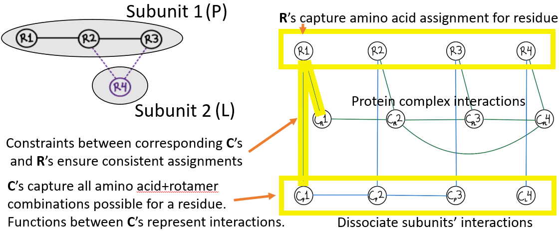
Figure 1: CPD formulated as a graphical model.

2.3 Graphical Model for K^*MAP

A discrete graphical model can be defined as a 3-tuple $\mathcal{M}\!=\!\langle\boldsymbol{X},\boldsymbol{D},\boldsymbol{F}\rangle$, where: $\mathbf{X}$ is a set of variables for which the model is defined; $\mathbf{D}\!=\!\{D_{X}\!:X\!\in\!\mathbf{X}\}$ is a set of finite domains, each defining the possible assignments for a variable; each $f_{\alpha}\in\mathbf{F}$ is a real-valued function defined over a subset of the model’s variables $\alpha\subseteq\mathbf{X}$ known as the function’s scope. More concretely, if we let $D_{\alpha}$ denote the Cartesian product of the domains of the variables in $\alpha$, then $f_{\alpha}\!:D_{\alpha}\!\rightarrow\mathbb{R}_{\geq 0}$. We let capital letters ($X$) represent variables and small letters ($x$) represent their assignment. Boldfaced capital letters (X) denote a collection of variables, $|{\bf X}|$ its cardinality, $D_{\boldsymbol{X}}$ its joint domain, and $\boldsymbol{x}$ a particular realization in that joint domain called a configuration. Operations denoted $\bigoplus_{\boldsymbol{X}}$ (ex. $\sum_{\boldsymbol{X}}$) imply $\bigoplus_{\boldsymbol{X}}\implies\bigoplus_{\boldsymbol{x}\in D_{\boldsymbol{X}}}$.

An important graphical model task that resembles K^* optimization is determination of the marginal maximum a-posteriori (or MMAP) (Definition 2.1, [Dechter, 2019]). Given the similarity, many graphical model algorithms for MMAP can be leveraged for K^* optimization.

Definition 2.1 (MMAP).

Given a graphical model $\mathcal{M}\!=\!\langle\boldsymbol{X},\boldsymbol{D},\boldsymbol{F}\rangle$, the marginal maximum a-posteriori of $\mathcal{M}$ is:

$$MMAP(\mathcal{M},\boldsymbol{Q}\subset\boldsymbol{X})=\max_{\boldsymbol{Q}}\sum_{\boldsymbol{S}=\boldsymbol{X}\setminus\boldsymbol{Q}}\prod_{\boldsymbol{F}}f(\boldsymbol{q},\boldsymbol{s})$$ (2)

Inspired by Viricel et al. [2018] and Vucinic et al. [2019], a recent formulation of CPD as graphical models was proposed by Pezeshki et al. [2022] as described below:

Variables and Domains:  The variables of the model consist of the union of two disjoint, but related, sets: a set of variables $\boldsymbol{R}$ representing the protein residue positions and a set of conformation variables $\boldsymbol{C}$ representing spatial orientation of the amino acids at each residue. More specifically, there are residue variables $\boldsymbol{R}=\{R_{i}\>|\>i\in\{1,2,...,N\}\}$, one for each of the $N$ protein residue being considered during the redesign. The respective domain of each $R_{i}$ consists of the amino acids being considered for its corresponding residue position. Each $R_{i}$ is accompanied by respective conformation variables $C_{\gamma(i)}$ representing the spatial conformation of the amino acid assigned to residue $R_{i}$ when the protein is in state $\gamma\in\boldsymbol{\varphi}=\{B,U\}$. Each $C_{\gamma(i)}$ has a domain $D_{C_{\gamma(i)}}=\{c\>|\>c$ is a rotamer for one of the possible amino acids of $R_{i}\}$. Thus, the amino acid assignment to $R_{i}$ acts as a selector into the possible assignments to $C_{\gamma(i)}$.

Functions:  Constraints $\boldsymbol{\mathscr{C}}=\{\mathscr{C}_{\gamma(i)}(R_{i},C_{\gamma(i)})\>|$ $i\in\{1,2,...,N\},\gamma\in\varphi\>\}$ ensure that the assigned rotamer to $C_{\gamma(i)}$ belongs to the amino acid assigned to $R_{i}$. Energy functions $E_{\gamma}^{sb}=\{E_{\gamma(i)}^{sb}(C_{\gamma(i)})\>|\>i\in\{1,2,...,N\}\}$ capture the energies of interaction of the amino acid at each residue $i$ with itself and the surrounding backbone. $E_{\gamma}^{pw}=\{E_{\gamma(ij)}^{pw}(C_{\gamma(i)},C_{\gamma(j)})\>|$ for $i,j$ s.t.​ $R_{i}$ and $R_{j}$ interact$\}$ capture pair-wise energies of interaction.

Objective: 
Let…

$$\begin{split}Z_{\gamma}(\boldsymbol{r})=\sum_{\boldsymbol{C}_{\gamma}}&\prod_{\boldsymbol{\mathscr{C}_{\gamma}}}\mathscr{C}_{\gamma(i)}(r_{i},c_{\gamma(i)})\>\\[-6.0pt] \cdot&\prod_{\boldsymbol{E_{\gamma}^{sb}}}e^{-\frac{E_{\gamma(i)}^{sb}(c_{\gamma(i)})}{\mathscr{R}T}}\>\\[-6.0pt] \cdot&\prod_{\boldsymbol{E_{\gamma}^{pw}}}e^{-\frac{E_{\gamma(ij)}^{pw}(c_{\gamma(i)},c_{\gamma(j)})}{\mathscr{R}T}}\end{split}$$ (3)

Objective Function:

$$K^{*}(\boldsymbol{r}) =\frac{Z_{B}(\boldsymbol{r})}{Z_{U}(\boldsymbol{r})},\hfill$$ (4)

Task:

$$K^{*}\textnormal{MAP} =\max_{\boldsymbol{R}}K^{*}(\boldsymbol{r}),\hfill$$ (5)

2.4 AOBB-K^* Algorithm

AOBB-K^* is an exact branch-and-bound algorithm proposed by Pezeshki et al. [2022] for optimization of K^*. AOBB-K^* constrains solutions such that the partition function of each protein subunit, $Z_{\gamma}$, is greater than a biologically-relevant subunit-stability threshold $S_{\gamma}$ as defined in [Ojewole et al., 2018]. The algorithm takes a CPD graphical model as input (Definition 2.2) and outputs the K^*MAP value of an optimal amino acid assignment to the residues. The algorithm is based on a class of AND/OR search algorithms over graphical models for optimization and inference tasks [Marinescu et al., 2014] and is empowered by constraint propagation.

Definition 2.2 (CPD Graphical Model).

Let $\mathcal{M}_{cpd}=\langle\boldsymbol{X}=\boldsymbol{R}\cup\boldsymbol{C},\;\boldsymbol{D},\;\boldsymbol{F}=\boldsymbol{\mathscr{C}}\cup\boldsymbol{E},\;\boldsymbol{S}\rangle$ be a CPD graphical model for K^*MAP optimization.

AOBB-K^* (Algorithm 1) traverses an underlying AND/OR search tree expanding nodes in a depth-first manner (line 1), and pruning whenever any of three conditions are triggered: (1) constraint propagation finds that the current assignments are inconsistent (line 1), (2) a subunit-stability constraint is violated (line 1), or (3) it can be asserted that the current amino acid configuration cannot produce a K^* better than any previously found (line 1). Backtracking occurs when all of a leaf node’s children have been explored and returned from (line 1), at which point the K^* value of the sub problem the node roots is known exactly and bounds of its parents are tightened accordingly. The algorithm progresses in this manner until it finally returns to, and updates, the root of the search tree with the maximal K^* value corresponding to an amino acid configuration that also satisfies the subunit-stability thresholds.

The version of AOBB-K^* used by Pezeshki et al. [2022] is guided by wMBE-K^*, a mini-bucket-based heuristic [Dechter and Rish, 2002] with cost-shifting [Liu and Ihler, 2011, Ihler et al., 2012], adapted for K^*MAP. wMBE-K^* is described in Algorithm 2 and operates similarly to its corresponding scheme for MMAP, wMBE-MMAP [Marinescu et al., 2014]. wMBE-K^* takes a variable ordering that constrains maximizations to be processed last (line 2). Functions are partitioned into the buckets $B_{k}$, and for any bucket $k$ with width larger than a provided i-bound (ie. when the number of distinct variables in the bucket’s functions is greater than the provided i-bound), a bounded approximation is made by partitioning the bucket functions into $T$ mini-buckets $MB_{k}^{(t)}$ (line 2) and taking a power-sum over the bucket variable (lines 2-2, 2-2, Definitions 2.3-2.4), leveraging Holder’s Inequality [Hardy et al., 1988].

Definition 2.3 (Consolidated Mini-Bucket Function).

Consider a mini-bucket $MB_{k}^{(t)}$. We define its consolidated mini-bucket function as $f_{MB_{k}^{(t)}}:=\prod_{f\in MB^{(t)}_{k}}f$

Definition 2.4 (Mini-Bucket Power Sum).

The power sum of a mini-bucket $MB_{k}^{(t)}$ is defined as $\sum_{X}^{w}f_{MB_{k}^{(t)}}:=(\sum_{X}(f_{MB_{k}^{(t)}})^{\frac{1}{w}})^{w}$.

Unlike wMBE-MMAP, buckets of wMBE-K^* corresponding to variables in $\boldsymbol{C_{U}}$, whose marginal belongs to the denominator of the K^* expression, are lower-bounded (to lead to an upper bound on K^*) by using a modification to Holder’s inequality that incorporates negative weights [Liu and Ihler, 2011] (lines 2-2). When messages are passed from buckets of $\boldsymbol{C_{U}}$ to that of $\boldsymbol{R}$ the messages are inverted to accommodate being part of the K^* denominator (line 2). Although details are omitted here, wMBE-K^* can also employ cost shifting to tighten its bounds (for more details see [Flerova et al., 2011, Liu and Ihler, 2011]).

Complexity.

The time complexity of AOBB-K^*’s search is exponential in the depth of the search tree, while the space complexity is linear in its depth. The time and space complexity of wMBE-K^* are exponential in the i-bound $i$.

input :  CPD graphical model $\mathcal{M}_{cpd}$ (Def 2.2);

pseudo tree $\mathcal{T}$ guiding node expansions;

$K^{*}$ upper-bounding heuristic function $h_{K^{*}}(.)$;

$Z_{\gamma}$ upper-bounding heuristic function $h_{Z_{\gamma}}(.)$

output :  $K^{*}MAP(\mathcal{M}_{cpd})$

1

2begin

3    

4    Encode deterministic relations in $\mathcal{M}_{cpd}$ into CNF

5    

6    $\pi\leftarrow$ search path initialized with a dummy root node $r$

7    

8    $H_{K^{*}}\leftarrow$ tables precomputed by $h_{K^{*}}(r)$

9    $H_{Z_{\gamma}}\leftarrow$ tables precomputed by $h_{Z_{\gamma}}(r)$ for each $\gamma$

10    while $EXPAND(\pi,\mathcal{T})$ do

11        

12        if $ConstraintPropagation(\pi)=false$ then

13             $PRUNE(\pi)$

14        

15        else if $\exists\gamma\in\varphi$ s.t. $ub_{Z_{\gamma}}(\pi,H_{Z_{\gamma}})<S_{\gamma}$ then

16             $PRUNE(\pi)$

17        

18        else if  $X\in\boldsymbol{R}$  then

19             if  $ub_{K^{*}}(\pi,H_{K^{*}})<lb_{K^{*}}$  then

20                 $PRUNE(\pi)$

21            

22        

23        while $\pi$ has no unexpanded children do

24             $BACKTRACK(\pi)$

25        

26    

27    return $lb_{K^{*}}=K^{*}MAP(\mathcal{M}_{cpd})$

28

Algorithm 1 AOBB-K^*

input :  CPD Graphical model $\mathcal{M}_{cpd}$ (Def 2.2);   i-bound $i$;

constrained variable order $d=[X_{1},...,X_{n}]$

output :  upper bound on the K^*MAP: $ub_{K^{*}\!MAP}(\mathcal{M}_{cpd})$

1

2begin

3     Partition the functions $f\in\boldsymbol{F}$ into buckets $B_{n},...,B_{1}$ s.t. each function is placed in the bucket corresponding to the highest-index variable in its scope.

4    foreach $k=n...1$ do

5         Generate a mini-bucket partitioning of the bucket functions $\boldsymbol{MB_{k}}=\{MB_{k}^{(1)},...,MB_{k}^{(T)}\}$ s.t. $|scope(f_{MB_{k}^{(t)}})|\leq i$, for all $MB_{k}^{(t)}\in\boldsymbol{MB_{k}}$

6        if $X_{k}\in\boldsymbol{MAP}$ then

7             foreach $MB^{(t)}_{k}\in\boldsymbol{MB_{k}}$ do

8                 $\lambda^{(t)}_{k}\leftarrow\max_{X_{k}}f_{MB_{k}^{(t)}}$

9            

10         else

11             if $X_{k}\in\boldsymbol{C_{B}}$ then // upper-bound for numerator

12                 Select positive weights $\boldsymbol{w}=\{w_{1},...,w_{T}\}$ s.t. $\sum_{w_{t}\in\boldsymbol{w}}w_{t}=1$

13                foreach $MB^{(t)}_{k}\in\boldsymbol{MB_{k}}$ do

14                     $\lambda^{(t)}_{k}\leftarrow\sum_{X_{k}}^{w_{t}}f_{MB_{k}^{(t)}}$

15                

16             else if $X_{k}\in\boldsymbol{C_{U}}$ then // lower-bound for denominator

17                 Select a negative weight $w_{1}$ and positive weights $\boldsymbol{w}=\{w_{2},...,w_{T}\}$ s.t. $\sum_{w_{t}\in\boldsymbol{w}}w_{t}=1$

18                foreach $MB^{(t)}_{k}\in\boldsymbol{MB_{k}}$ do

19                     $\lambda^{(t)}_{k}\leftarrow\sum_{X_{k}}^{w_{t}}f_{MB_{k}^{(t)}}$

20                    if $scope(\lambda^{(t)}_{k})\subseteq\boldsymbol{R}$ then

21                         $\lambda^{(t)}_{k}\leftarrow 1/\lambda^{(t)}_{k}$

22                    

23                

24            

25        Add each $\lambda^{t}_{k}$ to the bucket of the highest-index variable in its scope.

26    return $\lambda_{1}=ub_{K^{*}\!MAP}(\mathcal{M}_{cpd})$

27

Algorithm 2 wMBE-K^*

3 Boosting AOBB-K^*

The original AOBB-K^* algorithm presented by Pezeshki et al. [2022] showed promise with good performance compared to state-of-the-art BBK^* on small problems with rigid rotamers. However it suffered from scalability issues with its performance decreasing on problems with three mutable residues and being unable to solve problems with four or more mutable residues. In this paper we advance AOBB-K^* by presenting AOBB-K^*-b (boosted) with modifications to improve scalability. These enhancements, which are outlined below, are a mix of CPD domain-specific enhancements as well as principled enhancements that can be generalized to other graphical models tasks and problem domains.

3.1 Boosted wMBE-K^*

As noted by the authors of Pezeshki et al. [2022], a main cause of the scalability limitations of the AOBB-K^* was a sometimes weak or unbounded heuristic estimate by wMBE-K^* (Algorithm 2). This occurred primarily because of difficulties in the lower-bounding computations corresponding to the denominator of K^* and lead to loose upper bounds on the K^*MAP, or - in the case of a zero-valued lower bound - an all-together unbounded K^*MAP estimate. Such loose bounds (or lack of bounds) do not allow pruning during search, drastically enlarging the traversed search space.

To alleviate this, we introduce wMBE-K^*-b (boosted) with three sequential improvements to wMBE-K^*: (1) adjustment of the power-sum mechanism (lines 2,2) to produce non-zero lower-estimates at the cost of losing bound guarantees, (2) adjustment to the cost shifting mechanism to prevent cost-shifts with zeros, and (3) maximization with finite values over infinite ones (line 2). The specific adjustments and justifications for these modifications are explained next.

1) Enforcing non-zero lower estimates. wMBE-K^*, uses a power-sum computation (lines 2,2) leveraging Holder’s inequality to compute bounds (with a version using negative weights for lower bounding [Liu and Ihler, 2011]). Deriving inspiration from Domain-Partitioned MBE presented in Pezeshki et al. [2022] we adjust the computation to omit zeros in the lower-bounding power-sum (line 2) thus forcing non-zero estimates for consistent sub problems.

Definition 3.1 (Zero-Omitted Weighted Function).

The zero-omitted $w$ weighted function of a function $f$ with scope $\boldsymbol{Y}$ is: $f^{\triangleleft w}(y):=f(y)^{w}$ for $f(y)\neq 0$ and $0$ otherwise.

Definition 3.2 (Zero-Omitted Power Sum).

The zero-omitted power sum of a function $f$ that includes $X$ in its scope is: $\sum_{X}^{\triangleleft w}f:=(\sum_{X}f(x)^{\triangleleft\frac{1}{w}})^{w}$ where $\frac{0}{0}:=0$.

Specifically, line 2 is changed to: $\lambda^{t}_{k}\leftarrow\sum_{X_{k}}^{\triangleleft w}f_{MB_{k}^{(t)}}$.

This modified version can no longer guarantee a lower bound, however boundedness can be retained if the omitted zeros correspond to conditions for bounded domain-partitioning [Pezeshki et al., 2022]:

Theorem 3.1 (Bounded Domain-Partitioning).

Consider three variables $X$, $Y$, and $Z$ and objective

$$obj=\sum_{X}f(x,y)\cdot g(x,z)$$ (6)

Let $X^{\prime}=\{x\in X|g(x,z)\neq 0\}$ be a set such that $\epsilon_{X^{\prime}}=min_{x\in X^{\prime}}g(x,z)$. Since this makes $\epsilon_{X^{\prime}}>0$ we can derive:

$$obj= \sum_{x\in X^{\prime}}f(x,y)\!\cdot\!g(x,z)+\!\!\sum_{x\in X\setminus X^{\prime}}f(x,y)\!\cdot\!g(x,z)$$ (7)

$$= \sum_{x\in X^{\prime}}f(x,y)\!\cdot\!g(x,z)\;\;\geq\;\;\epsilon_{X^{\prime}}\!\cdot\!\sum_{x\in X^{\prime}}f(x,y)$$ (8)

$$\;> \;0$$ (9)

when $f(x,z)$ is not identically zero over $X^{\prime}$.

which allows for weighted mini-buckets to retain (and improve) bounds.

2) Cost shifting with non-zero values. We similarly adjust the cost-shifting mechanism (described in Flerova et al. [2011], Ihler et al. [2012]) restricting cost-shifts to be only with non-zero values. This again helps prevent numerical instabilities and ensures a positive lower bound for consistent sub problems. This does not disrupt bound guarantees.

3) Maximizing finite values. Due to the above-mentioned adjustments, the resulting K^* approximation for any [partial] configuration of the residues that are consistent will necessarily have a finite positive value (the upper bound estimates on the $K^{*}=\frac{Z_{B}}{Z_{U}}$ numerator are inherently finite and, now, the lower estimate of the denominator is also forced to be finite for consistent sub problems). Due to this result, during the maximization step (line 2), we can now instead maximize only over the available finite values.

3.2 Tuning search

Two key enhancements were also made to AOBB-K^* search.

Prioritizing the wild-type assignment. Unlike many other problem domains, when performing protein re-design a good initial assignment to the variables is known ahead of time: that which corresponds to the wild-type protein. Thus, we force the wild-type to be explored first, ensuring that we initialize our search with a powerful lower bound.

Prioritizing nodes with a finite heuristic value. Since wMBE-K^*-b produces infinite K^* estimates only for invalid configurations, we adjust node ordering during search to first explore nodes that have a finite heuristic value. This ensures that consistent configurations are traversed first.

In the Empirical Evaluation section we evaluate the performance impact of these changes.

4 Dynamic Heuristics

Next we explore using dynamic heuristic re-computations to improve bounds and enhance pruning during search (ex. [Lam et al., 2014]). AOBB-K^*-DH (Algorithm 3) is a general framework for dynamic heuristic use with AOBB-K^*.

AOBB-K^*-DH employs search similarly to AOBB-K^* with the exception that, at each node expansion not resulting immediately in pruning, there is a decision made whether or not to dynamically recompute a new K^* upper-bounding heuristic conditioned on the current search path (line 3). This decision is based on two hyper-parameters: $maxDepth$ (a maximum depth at which to consider recomputations) and $dhThreshold$ (a numerical bound on existing heuristic estimates over which re-computations occur). These hyper-parameters serve to regulate the frequency of dynamic heuristic re-computations since they can be costly both in time and memory. (In particular, wMBE-K^* is exponential in its $i\mathchar 45\relax bound$ hyper-parameter). When pruning or backtracking past the point of the most recent heuristic re-computation, the K^* heuristic tables $H_{K^{*}}$ are rolled back to cached tables from previous computations (not shown explicitly). Using an upper-bounding heuristic we have:

input :  CPD graphical model $\mathcal{M}_{cpd}$ (Def 2.2);

pseudo tree $\mathcal{T}$ guiding node expansions;

$K^{*}$ upper-bounding heuristic function $h_{K^{*}}(.)$;

$Z_{\gamma}$ upper-bounding heuristic function $h_{Z_{\gamma}}(.)$

output :  $K^{*}MAP(\mathcal{M}_{cpd})$

1

2begin

3    

4    Encode deterministic relations in $\mathcal{M}_{cpd}$ into CNF

5    

6    $\pi\leftarrow$ search path initialized with a dummy root node $r$

7    

8    $H_{K^{*}}\leftarrow$ tables precomputed by $h_{K^{*}}(r)$

9    $H_{Z_{\gamma}}\leftarrow$ tables precomputed by $h_{Z_{\gamma}}(r)$ for each $\gamma$

10    while $EXPAND(\pi,\mathcal{T})$ do

11        

12        if $ConstraintPropagation(\pi)=false$ then

13             $PRUNE(\pi)$

14        

15        else if $\exists\gamma\in\varphi$ s.t. $ub_{Z_{\gamma}}(\pi,H_{Z_{\gamma}})<S_{\gamma}$ then

16             $PRUNE(\pi)$

17        

18        else

19            

20            if $depth(\pi)\leq maxDepth$ and $H_{K^{*}}(\pi)>dhThreshold$ then

21                 $H_{K^{*}}\leftarrow$ tables recomputed by $h_{K^{*}}(\pi)$

22            

23            if  $X\in\boldsymbol{R}$  then

24                 if  $ub_{K^{*}}(\pi,H_{K^{*}})<lb_{K^{*}}$  then

25                     $PRUNE(\pi)$

26                

27            

28        

29        while $\pi$ has no unexpanded children do

30             $BACKTRACK(\pi)$

31        

32    

33    return $lb_{K^{*}}=K^{*}MAP(\mathcal{M}_{cpd})$

34

Algorithm 3 AOBB-K^*-DH

Theorem 4.1 (correctness, completeness).

AOBB-K^*-DH is sound and complete, returning the optimal K^* value of a corresponding amino-acid configuration that does not violate the subunit-stability constraints.

maxDepth.

The $maxDepth$ parameter ensures that dynamic heuristics are not recomputed past a predetermined depth, bounding the maximum number of times re-computation can occur, as demonstrated next.

Complexity of AOBB-K^*-DH wMBE-K^* Computations.

Since re-computation of the heuristic may occur anywhere in the search tree up to $maxDepth$ yielding exp($maxDepth$) number of nodes, and since each re-computation is $exp(i)$ given i-bound $i$, we can bound the time complexity as $O(k^{maxDepth+i})$, where $k$ is the maximum domain size encountered. However, the number of nodes explored during search can be far smaller due to pruning, and a tighter heuristic can further reduce the explored space. Letting $\Lambda_{DH}$ represent the number of nodes explored with DH, the time complexity bound can be expressed as $O(\Lambda_{DH}\cdot k^{i}$). If we let $\Lambda$ be the number of nodes explored without $DH$, the time complexities with and without DH are $O(\Lambda_{DH}\cdot k^{i})$ vs. $O(\Lambda)$ respectively. Thus, if $\frac{\Lambda}{\Lambda_{DH}}>k^{i}$ the use of DH will be cost-effective. Finally, since AOBB-K^* is a depth-first algorithm, the bound on the space overhead is linear in $maxDepth$ and $exp(i)$ for wMBE-K^*.

dhThreshold.

Dynamic heuristic re-computations aim to improve bounds and enhance pruning. However, if the existing heuristic value is already tight, the cost of re-computation may outweigh traversing the search space with the current heuristic. Determining what is considered "already tight" can be uncertain for general search tasks. However, in the case of protein re-design valid solutions must have a cost similar to the wild-type. Therefore, initially, we can provide $dhThreshold$ values relative to the native wild-type K^* value, improving them as better solutions emerge.

5 UFO: A Principled Scheme to Introduce Determinism

It is well known that utilizing constraint propagation (CP) as a tool for pruning inconsistent search paths can greatly speed up search Dechter [2019], Mateescu and Dechter [2008], Darwiche [2009]. Similar ideas have been explored in mixed integer programming [Danna et al., 2005]. More recently in the scope of protein design Pezeshki et al. [2022] demonstrated that introducing artificially generated determinism by underflowing function values under a provided threshold (Definition 5.1) can further leverage CP and enhance the speed of solving K^* optimization problems.

As our last set of algorithmic improvements we present 1) Algorithm 4: UFO (underflow-threshold optimization) describing a general methodology for choosing underflow-thresholds (Definition 5.1) with certain characterizations, and 2) AOBB-K^*-UFO, AOBB-K^* augmented with a CPD-specific UFO scheme.

Definition 5.1 ($\tau$-underflow of $f$, $f_{\tau}$).

Let $f$ be a non-negative function and $\tau\in\mathbb{R}^{+}$. The $\tau$-underflow of $f$ is $f_{\tau}(x)=f(x)$ if $f(x)\geq\tau$ and $0$, otherwise.

Definition 5.2 ($\tau$-underflow of $\mathcal{M}$, $\mathcal{M}_{\tau}$).

For $\mathcal{M}\!=\!\langle\mathbf{X,D,F}\rangle$, the $\tau$-underflow of $\mathcal{M}$ is $\mathcal{M}_{\tau}=\langle\mathbf{X,D,F_{\tau}}\rangle$, where $\mathbf{F_{\tau}}=\{f_{\tau}\;|\;f\in\boldsymbol{F}\}$.

5.1 Underflow-threshold Choice

1

input : Graphical model $\mathcal{M}=\langle\boldsymbol{X},\boldsymbol{D},\boldsymbol{F}\rangle$; SAT solving algorithm, $SAT(.)$ ; time limit for binary search; a deflation factor $0<\delta\leq 1$

output : A proposed threshold $\tau$ to use

2

3begin

4    

5    if $SAT(\mathcal{M})=False$ then

6         return $FAILURE$

7    

8    $\tau_{min}=0$;   $\tau_{max}=\max_{\boldsymbol{F},\boldsymbol{X}}f(\boldsymbol{x})$

9     $\tau=\frac{\tau_{max}+\tau_{min}}{2}$

10    

11    while time remains for $\tau$ binary search do

12         if $SAT(\mathcal{M_{\tau}})=False$ then

13             $\tau_{max}=\tau$

14            

15         else

16             $\tau_{min}=\tau$

17            

18         $\tau=\frac{\tau_{max}+\tau_{min}}{2}$

19        

20    

21    $\tau=\tau_{min}\cdot\delta$

22    

23    return $\tau$

24

Algorithm 4 UFO

Clearly larger underflow-thresholds lead to more determinism and consequently more aggressive CP pruning. However, if the threshold is set too high, the resulting model becomes inaccurate and may even become inconsistent leaving no configuration capable of producing a non-zero value.

Definition 5.3 (Inconsistent Model).

A model is said to be inconsistent if $\;\forall\boldsymbol{x}\in D_{\boldsymbol{X}},\;\prod_{\boldsymbol{F}}f(x)=0$.

Therefore it is useful to find a threshold that is as high as possible yet still results in a consistent model. To achieve this UFO employs binary search to find the largest threshold that still results in a satisfiable model (lines 4-4). Then UFO decreases the threshold using a hyper-parameter $\delta$ (line 14) to enable a wider array of solutions.

Note that UFO operates under the assumption that satisfiability of a model can be determined quickly. This is not true in general, nevertheless we have found that the satisfiability sub-task underlying many optimization problems tends to be easy. In other cases, satisfiability can be approximated by constraint propagation schemes [Dechter, 2003].

AOBB-K^*-UFO.

AOBB-K^*-UFO (Algorithm 5) empowers AOBB-K^* by generating an underflowed model ${\mathcal{M}_{cpd}}_{\tau}$ with $\tau$ determined by the UFO scheme specially adjusted for CPD, denoted UFO_cpd. This modified UFO_cpd performs underflows on the Boltzmann transformed $E^{sb}$ and $E^{pw}$ functions (see Equation 3) and replaces the general satisfiability check in the UFO algorithm (Algorithm 4, line 4) with one that enforces satisfiability of the wild-type sequence, thus ensuring a lower bound on the quality of solutions.

input : $\mathcal{M}_{cpd}$ (Def 2.2); $x_{wt}$, wild-type assignment to $X$; SAT solving algorithm, $SAT(.)$ ; time limit for binary search; a deflation factor $0<\delta\leq 1$; pseudo tree $\mathcal{T}$ guiding search; $K^{*}$ upper-bounding heuristic function $h_{K^{*}}(.)$; $Z_{\gamma}$ upper-bounding heuristic function $h_{Z_{\gamma}}(.)$;

output : approximation to the true $K^{*}MAP(\mathcal{M})$

1

2begin

3     $\tau\leftarrow UFO_{cpd}(\mathcal{M}_{cpd},x_{wt},SAT(.),time\mathchar 45\relax limit,\delta)$

4     $K^{*}{}^{\prime}\leftarrow AOBB{\text{-}}K^{*}({\mathcal{M}_{cpd}}_{\tau},\mathcal{T},h_{K^{*}}(.),h_{Z_{\gamma}}(.))$

5     return $K^{*}{}^{\prime}$

6

Algorithm 5 AOBB-K^*-UFO

UFO for other graphical model tasks.

As UFO is a general scheme, it can be useful for a myriad of graphical model tasks. A preliminary investigation into its use can be found in the report Exploring UFO’s.

6 Empirical Evaluation

6.1 Experimental methodology

Benchmarks.

We performed empirical evaluation on benchmarks derived from re-design problems for real proteins provided by the Bruce Donald Lab at Duke University. To gradually increase difficulty, small problems with two mutable residues (with five to ten total residues) were incrementally enlarged by making more of the residues mutable. Experiments were performed on the "Expanded" problem set from Pezeshki et al. [2022] consisting of 12 problems with 3 mutable residues, a new set of 32 problems expanded to have 4 mutable residues, and a set of 18 problems expanded to have 5 mutable residues. The names of the newly created benchmarks are shown with three parts: d[g]-[M]-[p] (eg. d27-4-1), where [g] represents the problem design number as obtained from the Donald Lab, [M] indicates the number of mutable residues after enlarging, and [p] is a single digit representing the specific permutation of the M residues that were made mutable. The resulting conformation spaces for these problems ranged from on the order of $10^{6}$ for 3 mutable residues to $10^{11}$ for 5 mutable residues.

Algorithms.

We experimented with 5 algorithms: AOBB-K^*; AOBB-K^*-b (boosted) with an improved wMBE-K^*-b heuristic and search enhancements (Section 3); AOBB-K^*-b-DH, AOBB-K^*-b with dynamic heuristics (Section 4); AOBB-K^*-b-UFO, AOBB-K^*-b empowered with a CPD-specific UFO scheme (Section 5); and BBK^*, state-of-the-art best-first search algorithm in comprehensive CPD software OSPREY 3.0 [Ojewole et al., 2018, Hallen et al., 2018].

Each AOBB-K^* derived algorithm was implemented in C++. AOBB-K^*-b-DH dynamic heuristic re-computations were regulated with $maxDepth=2$ and $dhThreshold=10^{20}\cdot K^{*}_{wt}$, where $K^{*}_{wt}$ is the wild-type K^* value. The UFO scheme used by AOBB-K^*-b-UFO performed binary search in log-space and decreased the resulting threshold with $\delta=0.2$ (Algorithm 4: UFO, line 4). Because the AOBB-K^*-b algorithms use the wMBE-K^*-b heuristic which does not guarantee bounds, they do not guarantee discovery of the optimal K^* (ie. they are not complete). Similarly, schemes empowered with UFO lose optimality guarantees.

BBK^* is implemented in Java, was set to use rigid rotamers, and given a bound-tightness of $1\times 10^{-200}$^[]. Despite the extremely small bound tightness parameter, BBK^* still performs noticeably as an approximate algorithm.

Experiments were run on a 2.66 GHz processor, and given 4 GB of memory and a time limit of 1hr for each problem. As BBK^* can take advantage of parallelism, it was given access to 4 CPU cores.

6.2 Results

Comparing AOBB-K^*-b vs AOBB-K^*.

In Table 1 we examine performance of AOBB-K^*-b (with tightened wMBE-K^*-b) vs. AOBB-K^* on the "Expanded" benchmark set from Pezeshki et al. [2022] with three mutable residues. We compare solution quality and speed of the two algorithms. The i-bound of AOBB-K^*-b was set to $i=4$. For AOBB-K^* we use the best performing i-bound as reported previously. We highlight in blue any better K^* solutions and any significantly faster completion times (equal to or under 80% of the competing algorithm’s completion time). The wild-type K^* value ("wt K^* ​") is also shown.

The highlighted blue times show AOBB-K^*-b finishing significantly faster for half of the problems. It also solves a problem that AOBB-K^* could not. Finally, AOBB-K^*-b is able to find the optimal solution for each of these problems (although it does not prove optimality).

List of tablefigures 1 Performance of AOBB-K^*-b vs AOBB-K^* on benchmarks with 3 mutable residues from Pezeshki et al. [2022]. Displayed are the i-bound ("i") used by each, their respective best-found K^* value ("Soln"), their completion time ("Time"), and, as reference, the wild-type K^* value ("wt K^* ").

Evaluating Dynamic Heuristics.

Table 2 compares AOBB-K^*-b with and without the dynamic heuristic scheme described in Section 4 on problems with 3 or 4 mutable residues that both algorithms found optimal solutions for within an hour. We compare the size of the explored search space between the two algorithms (counting the number of OR and AND nodes of the residue variables traversed) and highlight when there are differences.

We see that dynamic heuristic re-computation reduces the size of the traversed search space in the majority of problems. In two cases (highlighted in red) dynamic heuristics cause an increase in the search space. This may occur when dynamic heuristic re-computation causes the K^* estimate for a node to increase (specifically by decreasing the denominator $Z_{U}$ estimate which wMBE-K^*-b does not guarantee to be a lower bound), preventing the node from being pruned.

List of tablefigures 2 Comparison of the explored search space by AOBB-K^*-b with and without use of a dynamic heuristic. Displayed are the respective i-bounds ("i") used, best-found K^* solutions ("Soln"), completion times ("Time"), and the size of the traversed AND/OR search space (number of residue OR and AND nodes).

UFO Impact and Cross Comparisons.

Table 3 compares the performance of AOBB-K^*-b-UFO, AOBB-K^*-b-DH, AOBB-K^*-b, and BBK^* on problems with three, four, and five mutable residues. The AOBB-K^*-based algorithms are displayed in a top-down ranking per problem, with the best ranking algorithm placed at the top. Ranking is based first on the quality of K^* found and then by the speed at which their respective solution was first discovered (measured in seconds and denoted "Anytime", highlighting the anytime nature of AOBB-K^* search). Large text highlights the value responsible for the algorithm’s higher ranking, and blue color indicates that BBK^* was outperformed.

From the rank-based ordering of the algorithms, the competitiveness of the UFO scheme is apparent. The frequency of blue coloring shows the algorithms’ competitiveness against BBK^* on the problems with three and four mutable residues. On problems having 5 mutable residues the AOBB-K^*-b schemes begin to struggle. This is likely due to the loss of bounds from the boosted modifications of wMBE-K^*-b in conjunction with a low i-bound, heavy underflows, and longer message passing for these larger problems. Nevertheless, AOBB-K^*-UFO is still able to find good solutions, sometimes better than that of BBK^*.

We also see the potential of the AOBB-K^*-DH scheme in terms of run-time in Table 3. On many problems shown, AOBB-K^*-b-DH performs better than AOBB-K^*-b (sometimes due to a better solution found, other times due to finding good solutions faster). However, AOBB-K^*-b-DH’s performance with respect to AOBB-K^*-b is less homogeneous when including the easier problems from Table 2 which were omitted from Table 3.

Finally, although AOBB-K^*-b generally ranked lower than the other AOBB-K^*-b variants, it keeps up with BBK^* through problems with 4 mutable residues (previously out of range for AOBB-K^*), and even finds respectable solutions for some 5-mutable-residue problems.

List of tablefigures 3 Comparison of the AOBB-K^*-b-[UFO/DH] schemes and BBK^* on problems ranging from 3 to 5 mutable residues. Shown is the i-bound used, best-found K^* solution (recomputed without underflow-thresholding), the time at which the best-found solution was first discovered ("Anytime"), and the completion time ("Time"). For reference, the wild-type K^* solution is also shown.

Determinism. A major factor that can lead to decreased performance on large problem for AOBB-K^* schemes (eg. problem d7-5-3) is that domain sizes increase significantly with an increasing number of mutable residues. This restricts wMBE-K^* to using lower i-bounds and reduces its accuracy. For example, AOBB-K^* could use an i-bound of 4 for problems with 3 mutable residues, but was restricted to an i-bound of 3 for problems with 5 mutable residues in Table 3. To explore the potential of moving to more compact representations that could enable use of higher i-bounds, determinism in wMBE-K^*-b’s computed messages for AOBB-K^*-b-UFO were evaluated. For problems with 5 mutable residues, the largest tables generated by wMBE-K^*-b often had a determinism ratio of > 0.95 - namely 95% of the entries were zeros. This insight adds motivation to moving to other representations that can take advantage of the repeated determinism, such as relational representations.

Summary of Empirical Results. AOBB-K^*-b, AOBB-K^*-b-DH, and AOBB-K^*-b-UFO have now achieved scalability to problems with 5 mutable residues. The UFO scheme demonstrated strong performance in particular, competitive with BBK^* for these problems. Analysis of AOBB-K^*-b-DH’s explored search space shows its promise, but the current naive implementation showed limited performance on larger problems. Lastly, analysis of wMBE-K^*-b in the presence of UFO revealed a high level of determinism indicating that more compact representations may be beneficial. (Additional results can be found in the Supplemental Materials).

7 Conclusion and Future Directions

Conclusion. This work introduced several improvements to the protein re-design algorithm AOBB-K^* to enhance its scalability. Refinements to its wMBE-K^* heuristic were presented sacrificing bound guarantees for tighter estimates, and adjustments were made to its node value-ordering strategy during search. These enhancements were implemented in AOBB-K^*-b (boosted) which scaled up to problems with 5 mutable residues whereas AOBB-K^* could only produce solutions to problems with 3 mutable residues. To further enhance pruning during search, the dynamic heuristic scheme AOBB-K^*-DH was introduced. Evaluation with a naive implementation showed the promise of dynamic heuristics being incorporated into AOBB-K^*. Additionally, UFO - a new underflow-thresholding scheme for introducing artificial determinism to strengthen constraint propagation - was introduced. A specialized version of UFO for CPD was incorporated into AOBB-K^*-b as AOBB-K^*-b-UFO and showed competitive performance against state-of-the-art BBK^* on problems of up to 5 mutable residues. Evaluation of these algorithms was done using 62 real-protein benchmarks involving three to five mutable residues.

Future Directions. We leave the following as future directions: to 1. investigate modifications to wMBE-K^*-b that mitigate the risk of violating boundedness; 2. adapt richer implementations of dynamic heuristics [Lam et al., 2014]; 3. consider look-ahead schemes [Lam et al., 2017]; 4. extend to finding the n-best K^*’s such as approaches by Flerova et al. [2016], Ruffini et al. [2021]; 5. investigate the trade-offs of the dynamic heuristic hyper-parameters; 6. explore UFO utility in other graphical model tasks; 7. explore more compact representations of wMBE-K^* that can take advantage of the high levels of determinism [Mateescu and Dechter, 2008, Larkin and Dechter, 2003] or other scalable heuristics [Lee et al., 2016]; 8. apply the proposed approaches to real biological tasks; 9. extend these algorithms by incorporating other state-of-the-art inference schemes, especially approximate schemes [Yanover and Weiss, 2002, Hurley et al., 2016, Lou et al., 2018a, b, Marinescu et al., 2019, 2018a, 2018b].

Acknowledgements

Thank you to reviewers of this paper for their valuable comments and suggestions. We also acknowledge use of ChatGPT, an AI language model developed by OpenAI, in refining text. This work was supported in part by NSF grant IIS-2008516.

References

- Al-Lazikani et al. [2001] Bissan Al-Lazikani, Joon Jung, Zhexin Xiang, and Barry Honig. Protein structure prediction. Current Opinion in Chemical Biology, 5(1):51–56, 2001.
- Danna et al. [2005] Emilie Danna, Edward Rothberg, and Claude Le Pape. Exploring relaxation induced neighborhoods to improve mip solutions. Mathematical Programming, 102:71–90, 2005.
- Darwiche [2009] Adnan Darwiche. Modeling and Reasoning with Bayesian Networks. Cambridge University Press, 2009.
- Dauparas et al. [2022] Justas Dauparas, Ivan Anishchenko, Nathaniel Bennett, Hua Bai, Robert J Ragotte, Lukas F Milles, Basile IM Wicky, Alexis Courbet, Rob J de Haas, Neville Bethel, et al. Robust deep learning–based protein sequence design using proteinmpnn. Science, 378(6615):49–56, 2022.
- Dechter [2003] Rina Dechter. Constraint Processing. Morgan Kaufmann, 2003.
- Dechter [2019] Rina Dechter. Reasoning with probabilistic and deterministic graphical models: Exact algorithms, second edition. Synthesis Lectures on Artificial Intelligence and Machine Learning, 13:1–199, 02 2019.
- Dechter and Rish [2002] Rina Dechter and I Rish. Mini-buckets: A general scheme for approximating inference. Journal of the ACM, pages 107–153, 2002.
- Defresne et al. [2021] Marianne Defresne, Sophie Barbe, and Thomas Schiex. Protein design with deep learning. International Journal of Molecular Sciences, 22(21), 2021.
- Donald [2011] Bruce Donald. Algorithms in structural molecular biology. MIT Press, 2011.
- Flerova et al. [2011] Natalia Flerova, Alexander Ihler, Rina Dechter, and Lars Otten. Mini-bucket elimination with moment matching. In Workshop on Discrete Optimization in Machine Learning (DISCML) at NIPS, 2011.
- Flerova et al. [2016] Natalia Flerova, Radu Marinescu, and Rina Dechter. Searching for the M best solutions in graphical models. J. Artif. Intell. Res., 55:889–952, 2016.
- Gainza et al. [2016] Pablo Gainza, Hunter M Nisonoff, and Bruce R Donald. Algorithms for protein design. Current opinion in structural biology, 39:16–26, 2016.
- Hallen et al. [2018] Mark Hallen, Jeffrey Martin, Adegoke Ojewole, Jonathan Jou, Anna Lowegard, Marcel Frenkel, Pablo Gainza, Hunter Nisonoff, Aditya Mukund, Siyu Wang, Graham Holt, David Zhou, Elizabeth Dowd, and Bruce Donald. Osprey 3.0: Open-source protein redesign for you, with powerful new features. Journal of Computational Chemistry, 39, 10 2018.
- Hallen and Donald [2019] Mark A. Hallen and Bruce R. Donald. Protein design by provable algorithms. Commun. ACM, 62(10):76–84, sep 2019.
- Hardy et al. [1988] G.H. Hardy, J.E. Littlewood, and G. Pólya. Inequalities. Cambridge Mathematical Library. Cambridge University Press, 1988.
- Hill [1987] Terrell Hill. Statistical mechanics : principles and selected applications. Dover Publications, 1987.
- Hurley et al. [2016] Barry Hurley, Barry O’sullivan, David Allouche, George Katsirelos, Thomas Schiex, Matthias Zytnicki, and Simon de Givry. Multi-language evaluation of exact solvers in graphical model discrete optimization. Constraints, 21:413–434, 2016.
- Ihler et al. [2012] Alexander. Ihler, Natalia Flerova, Rina Dechter, and Lars Otten. Join-graph based cost-shifting schemes. In UAI, pages 397–406, 2012.
- Jumper et al. [2021] John Jumper, Richard Evans, Alexander Pritzel, Tim Green, Michael Figurnov, Olaf Ronneberger, Kathryn Tunyasuvunakool, Russ Bates, Augustin Žídek, Anna Potapenko, et al. Highly accurate protein structure prediction with alphafold. Nature, 596(7873):583–589, 2021.
- Lam et al. [2014] William Lam, Kalev Kask, Rina Dechter, and Alexander Ihler. Beyond static mini-bucket: Towards integrating with iterative cost-shifting based dynamic heuristics. In Seventh Annual Symposium on Combinatorial Search, 2014.
- Lam et al. [2017] William Lam, Kalev Kask, Javier Larrosa, and Rina Dechter. Residual-guided look-ahead in AND/OR search for graphical models. J. Artif. Intell. Res., 60:287–346, 2017.
- Larkin and Dechter [2003] David Larkin and Rina Dechter. Bayesian inference in the presence of determinism. AI and Statistics(AISTAT03), 2003.
- Lee et al. [2016] Junkyu Lee, Radu Marinescu, Rina Dechter, and Alexander Ihler. From exact to anytime solutions for marginal map. AAAI’16, page 3255–3262. AAAI Press, 2016.
- Lilien et al. [2004] Ryan H. Lilien, Brian W. Stevens, Amy C. Anderson, and Bruce R. Donald. A novel ensemble-based scoring and search algorithm for protein redesign, and its application to modify the substrate specificity of the gramicidin synthetase a phenylalanine adenylation enzyme. In Proceedings of the Eighth Annual International Conference on Research in Computational Molecular Biology, RECOMB ’04, page 46–57. Association for Computing Machinery, 2004.
- Liu and Ihler [2011] Qiang Liu and Alexander Ihler. Bounding the partition function using Hölder’s inequality. In International Conference on Machine Learning (ICML), pages 849–856. ACM, June 2011.
- Lou et al. [2018a] Qi Lou, Rina Dechter, and Alexander Ihler. Anytime anyspace and/or best-first search for bounding marginal map. Proceedings of the AAAI Conference on Artificial Intelligence, 32(1), 2018a.
- Lou et al. [2018b] Qi Lou, Rina Dechter, and Alexander. Ihler. Finite-sample bounds for marginal MAP. In Proceedings of the Thirty-Fourth Conference on Uncertainty in Artificial Intelligence, UAI 2018, Monterey, California, USA, August 6-10, 2018, pages 725–734. AUAI Press, 2018b.
- Marinescu et al. [2014] Radu Marinescu, Rina Dechter, and Alexander Ihler. And/or search for marginal map. In Proceedings of the Thirtieth Conference on Uncertainty in Artificial Intelligence, UAI’14, page 563–572. AUAI Press, 2014.
- Marinescu et al. [2018a] Radu Marinescu, Rina Dechter, and Alexander Ihler. Stochastic anytime search for bounding marginal map. In IJCAI, pages 5074–5081, 2018a.
- Marinescu et al. [2018b] Radu Marinescu, Junkyu Lee, Rina Dechter, and Alexander Ihler. And/or search for marginal map. J. Artif. Int. Res., 63(1):875–921, sep 2018b.
- Marinescu et al. [2019] Radu Marinescu, Akihiro Kishimoto, Adi Botea, Rina Dechter, and Alexander Ihler. Anytime recursive best-first search for bounding marginal map. Proceedings of the AAAI Conference on Artificial Intelligence, 33(01):7924–7932, Jul. 2019.
- Mateescu and Dechter [2008] Robert Mateescu and Rina Dechter. Mixed deterministic and probabilistic networks. Annals of mathematics and artificial intelligence, 54(1):3–51, 2008.
- McQuarrie [2000] Donald McQuarrie. Statistical mechanics. University Science Books, 2000.
- Moult et al. [2022] John Moult, Krzysztof Fidelis, Andriy Kryshtafovych, Torsten Schwede, Maya Topf, David Baker, Michael Feig, Nick Grishin, Andrzej Joachimiak, David Jones, and et al. 15th community wide experiment on the critical assessment of techniques for protein structure prediction, 2022.
- Ojewole et al. [2018] Adegoke Ojewole, Jonathan D. Jou, Vance G. Fowler, and Bruce Randall Donald. BBK* (Branch and Bound Over K*): A provable and efficient ensemble-based protein design algorithm to optimize stability and binding affinity over large sequence spaces. J. Comput. Biol., 25(7):726–739, 2018.
- Pezeshki et al. [2022] Bobak Pezeshki, Radu Marinescu, Alexander Ihler, and Rina Dechter. AND/OR branch-and-bound for computational protein design optimizing K*. In James Cussens and Kun Zhang, editors, Proceedings of the Thirty-Eighth Conference on Uncertainty in Artificial Intelligence, volume 180 of Proceedings of Machine Learning Research, pages 1602–1612. PMLR, 01–05 Aug 2022.
- Rossotti and Rossotti [1961] F.J.C. Rossotti and H. Rossotti. The Determination of Stability Constants: And Other Equilibrium Constants in Solution. McGraw-Hill series in advanced chemistry. McGraw-Hill, 1961.
- Ruffini et al. [2021] Manon Ruffini, Jelena Vucinic, Simon de Givry, George Katsirelos, Sophie Barbe, and Thomas Schiex. Guaranteed diversity and optimality in cost function network based computational protein design methods. Algorithms, 14(6), 2021.
- Viricel et al. [2018] Clement Viricel, Simon de Givry, Thomas Schiex, and Sophie Barbe. Cost function network-based design of protein-protein interactions: predicting changes in binding affinity. Bioinformatics (Oxford, England), 34, 02 2018.
- Vucinic et al. [2019] Jelena Vucinic, David Simoncini, Manon Ruffini, Sophie Barbe, and Thomas Schiex. Positive multistate protein design. Bioinformatics (Oxford, England), 36, 06 2019.
- Yanover and Weiss [2002] Chen Yanover and Yair Weiss. Approximate inference and protein-folding. Advances in neural information processing systems, 15, 2002.
- Zhou et al. [2016] Yichao Zhou, Yuexin Wu, and Jianyang Zeng. Computational protein design using and/or branch-and-bound search. Journal of computational biology : a journal of computational molecular cell biology, 23, 05 2016.