Kinematic anisotropies and pulsar timing arrays
Gianmassimo Tasinato1,2
1 Dipartimento di Fisica e Astronomia, Università di Bologna, Italia
2 Physics Department, Swansea University, SA28PP, United Kingdom
email: g.tasinato2208 at gmail.com
Abstract
Doppler anisotropies, induced by our relative motion with respect to the source rest frame, are a guaranteed property of stochastic gravitational wave backgrounds of cosmological origin. If detected by future pulsar timing array measurements, they will provide interesting information on the physics sourcing gravitational waves, which is hard or even impossible to extract from measurements of the isotropic part of the background only. We analytically determine the pulsar response function to kinematic anisotropies, including possible effects due to parity violation, to features in the frequency dependence of the isotropic part of the spectrum, as well as to the presence of extra scalar and vector polarizations. For the first time, we show how the sensitivity to different effects crucially depends on the pulsar configuration with respect to the relative motion among frames. Correspondingly, we propose examples of strategies of detection, each aimed at exploiting future measurements of kinematic anisotropies for characterizing distinct features of the cosmological gravitational wave background.
1 Introduction
Four pulsar timing array (PTA) collaborations [1, 2, 3, 4] recently detected a signal compatible with a stochastic gravitational wave background (SGWB). At the moment, various open questions remain on the origin of the gravitational wave (GW) signal, since diverse sources, from astrophysical to cosmological, are compatible with current observations (see e.g. [5] for a recent multi-model assessment). Properties of the SGWB can in principle allow us to distinguish astrophysical from cosmological sources of GW: parity violation [6, 7, 8, 9, 10, 11, 12, 13, 14, 15, 16, 17, 18], non-Gaussianities (see e.g. [19, 20, 21, 22]), or anisotropies (see [23] for a recent survey). If the SGWB has cosmological origin, besides its intrinsic anisotropies, the signal is expected to be characterised by a Doppler anisotropy due to our relative motion with respect to the source rest frame. As found by cosmic microwave background (CMB) experiments [24, 25, 26, 27], our velocity with respect to the cosmic rest frame has an amplitude of size with respect to the velocity of light, and points in the direction . Correspondigly, the size of the dipolar kinematic anisotropy of a cosmological SGWB should be one-thousandth smaller than the amplitude of the isotropic part of the GW spectrum. This is smaller in size than the expected anisotropies of the astrophysical SGWB in the PTA band (see e.g. [28, 29, 30, 31, 32] and in particular [33] for a recent study). But, as for the CMB, it is potentially well larger than intrinsic cosmological anisotropies (see, e.g., the studies [34, 35, 36, 37, 38, 39, 40]). Kinematic anisotropies is a topic of active research in the context of GW interferometers [23, 41, 42, 43, 44, 45]. It is then worth asking what information we can obtain from a possible future detection of kinematic anisotropies with PTA experiments.
This is the scope of this work. The development and refinement of detection techniques of anisotropies of SGWB from PTA observations have a long history – see e.g. [46, 47, 48, 49, 50, 51, 52, 53] – often borrowing and elaborating techniques developed in the context of ground-based [54, 55, 56, 57, 58] and space-based [59, 60, 61, 62, 63] interferometers. Current PTA measurements do not find yet indications of SGWB anisotropies [64, 65], but as data are becoming more and more accurate, a detection might be forthcoming (see also [66, 67, 68] for recent studies of related aspects of GW observations with PTA). Since in this work we specialize to kinematic anisotropies, we express our findings in the most convenient way to extract information from a detection of Doppler effects in the SGWB. We stress the geometrical aspects of the problem, and we make manifest how the sensitivity to different GW effects depends on the position of pulsars with respect to the relative velocity vector among frames. These findings – of which many are new while others are known but we set them in a new perspective – can be useful to plan future PTA observations. In fact, as we can plan the location of ground based interferometers in the Earth in order to extract most physics from observations (for example, see the recent study [69] in the context of the Einstein Telescope), we can also plan which pulsars are worth monitoring to learn new physics from GW measurements. This is an invaluable opportunity for forthcoming observations with SKA facilities, which will monitor and detect signals from a large number of pulsars [70] with important opportunities for GW physics: see e.g. [71]. The physical effects we explore using SGWB kinematic anisotropies in PTA band are:
-
Parity violation: Well motivated early-universe scenarios predict the existence of parity-violating effects in gravitational and gauge-field interactions, with interesting cosmological and GW consequences, see e.g. [6, 7, 8, 9, 10, 11, 12, 13, 14, 15, 16, 17, 18]. These effects manifest as circular polarization of the SGWB. This quantity is hard or even impossible to detect with single interferometers, when focussing on the isotropic part of the background only: see e.g. the clear analysis of [72]. Opportunities of detection arise when cross correlating different experiments, see e.g. [73, 74, 75], or by probing anisotropies of the SGWB: [76, 77, 78, 79]. For the case of PTA measurements, [80] shown for the first time that one needs to measure SGWB anisotropies for being sensitive to circular polarization (see also [81]). In our work, we show that kinematic anisotropies are in fact potentially able to probe circular polarization with PTA detections, and the PTA sensitivity depends on the pulsar location with respect to the relative motion along frames. Hence, a careful plan of the pulsars to monitor is needed for increasing opportunities to detection (see sections 2, 3, and 5).
-
Frequency features in GW spectrum: Kinematic anisotropies are obtained from Doppler boosting the isotropic part of the SGWB: they depend on derivatives along frequency of this quantity [41]. Hence, Doppler effects can be a complementary probe of the frequency dependence of the SGWB, alternative to more direct methods (see e.g. [82]). Kinematic anisotropies are more pronounced if the SGWB has features in frequency: suitable combinations of PTA anisotropy measurements allow us to specifically detect the slope of the background (see sections 3, and 5).
-
Presence of extra scalar and vector polarizations: Alternative theories of gravity predict the existence of additional scalar and vector polarizations with respect to the spin-2 ones of General Relativity (see e.g. [83] for a general discussion, and [84] for a comprehensive review). Previous works investigated how PTA measurements can probe the GW polarization content, see e.g. [85, 86, 87, 88, 89, 90, 91]. Here we point out that kinematic anisotropies, which depend on the slope of the spectrum, can be sensitive to extra polarizations also when the latter give a small contribution to the isotropic part of the spectrum (see sections 4, and 5).
We discuss the motivations and theoretical formulation of these topics in sections 2, 4 and 3, while in section 5 we elaborate strategies of detection of the effects listed above. Two Appendixes develop technical tools needed in the main text.
2 Set-up
In this section we investigate the response of a PTA experiment to an anisotropic SGWB characterized by the GW intensity and GW circular polarization. We will start appreciating how the PTA response to GW depend on the pulsar configuration. In the next sections, the resulting formulas will then be applied to the specific case of kinematic anisotropies.
The GW is expressed in terms of fluctuations of the Minkowski metric
| (2.1) |
We decompose the GW in Fourier modes as
| (2.2) |
imposing the condition
| (2.3) |
which ensures that is real. We also assume that the polarization tensors are real quantities. See Appendix A for more details on our conventions. The presence of a GW deforms the geodesics of light, and produces a time delay on the period of a pulsar. We denote with the time travelled from a pulsar to the Earth, setting from now on . The pulsar is situated at the position (from now on, hat quantities correspond to unit vectors)
| (2.4) |
with respect to the Earth, located at . The direction of the vector of the pulsar with respect to the Earth plays an important role for our arguments.
The time delay of the light geodesics reads
| (2.5) | |||||
| (2.6) |
is the so-called detector tensor, controlling the connection between the light delay 111 In writing eq (2.6), we neglect as usual the ‘pulsar terms’ and focus on the ‘Earth terms’. We refer the reader to Chapter 23 of [92] and to the recent [93] for textbook discussions on the quantities we are introducing, their physical properties, and more general information on how PTA respond to GW physics. and the GW:
| (2.7) |
Starting from the time delay , it is convenient to compute the time residual
| (2.8) |
which is easier to handle when Fourier transforming the signal. We assume that the correlators of Fourier modes of GW fluctuations can be expressed as
| (2.9) |
where the tensor defines the properties of the SGWB, and is the polarization index (we adopt a basis for the polarization tensors, see Appendix A). The quantity can be decomposed in intensity and circular polarization as
| (2.10) |
where the tensor is defined as , while . The SGWB intensity is real and positive, and the circular polarization is a real quantity. Both quantities can depend on the GW frequency and direction, and behave as scalars under boosts. Our aim is to compute the response of a PTA system to the presence of a SGWB, whose spectrum is characterized by (possibly anisotropic) intensity and circular polarization parameters.
In order to do so, we compute the correlation among the time residuals of a pair of pulsars, denoted respectively by the letters and , which is induced by the presence of GW. The correlations among time-residuals is essential for detecting and characterizing the SGWB [94]. We introduce the short-hand notation
| (2.11) |
and compute the two-point correlators of the the two pulsar time delays (we sum over repeated polarization indexes):
Making appropriate changes of variable, and , we can use relation (2.3) to recast the previous expression in a convenient form, which allows us to apply eq (2.9):
The previous result can be plugged in eq (2.8) to compute the two-point function of time residuals:
| (2.14) | |||||
where is the isotropic value of the intensity integrated over all directions, while is its analog for circular polarization.
The response functions of a pulsar pair to the GW intensity and circular polarization are obtained integrating over , and read
| (2.15) | |||||
| (2.16) |
These quantities depend on the relative position of the pulsars in the sky (given the dependence of the quantities on the pulsar location) and on the properties of the SGWB. Hence, the response of a PTA system to GW depends on the pulsar configuration. Notice that only correlators (2.14) evaluated at different times and are sensitive to circular polarization. In actual measurements though, correlators are weighted by suitable filters to better extract the signal. We discuss in Appendix B and section 5 the relation between correlators as above and measurable GW signals, using a a match-filtering technique.
Our task 222While in this section and the next we focus on spin-2 GW modes, the same procedure can be applied to study alternative gravity models in which gravitation is mediated by a mixture of spin-2 and spin-0 or spin-1 fields. We examine this possibility in section 4. is to compute and . The results depend also on the theory of gravity one considers. For the case GW are carried by spin-2 fields, as in General Relativity, we can make use of eqs (A.14) and (A.15). The quantities within parenthesis 333Formulas similar to (2.17) have been used in [52, 53] to characterize scenarios with anisotropic GW intensity. See also the treatment in [46]. As far as we are aware, our formulas for circular polarization are instead new in this context. in eqs (2.15) and (2.16) result:
| (2.17) | |||||
and
| (2.18) |
where denotes cross product among vectors. Plugging these results in eqs (2.15), (2.16), we are left with angular integrals to carry on, which depend on and . The computation gives quantities depending on the GW frequency. We can already notice that, being the quantity in eq (2.18) an odd function of the vector directions, the integral over all directions give zero, unless the circular polarization function depend explicitly on the direction . Hence we need an anisotropic signal to measure circular polarization [80, 81], completely analogously to what happens for planar interferometers (see e.g. [72]).
Starting from these basic formulas, in the next section we apply them to the specific case of spin-2 GW (including circular polarization), and study anisotropies induced by the motion of our reference frame with respect to the rest frame of the SGWB source.
3 PTA response to kinematic anisotropies: the spin-2 case
In the previous section we developed a general treatment to investigate the PTA response to anisotropic GW signals. We now specialise our attention to the case of Doppler anisotropies, in theories as General Relativity where GW are characterized by spin-2 polarizations. Nevertheless, we include also possible effects of parity violation [6, 7, 8, 9, 10, 11, 12, 13, 14, 15, 16, 17, 18]. The geometrical dependence of the PTA response to kinematic anisotropies make them a promising probe of the source of GW and of the physics of gravitation.
In fact, kinematic anisotropies are a guaranteed property of a SGWB of primordial origin: their features are fully calculable, being determined by the properties of the isotropic part of the SGWB. If the SGWB has a cosmological origin related with early-universe physics, we can expect that the relative motion among frames induces an effect analog to the large dipolar anisotropy measured in the CMB [24, 25, 26, 27], whose amplitude is a factor times smaller than the isotropic background. For the case of the CMB, the dipolar kinematic anisotropy is well larger in size than its intrinsic anisotropies. The same can occur for a cosmological SGWB detectable with PTA. For this reason it is worth characterizing kinematic effects, and explore what information we can extract from their detection with PTA experiments. We now show how the pulsar response to Doppler anisotropies depends on the pulsar location in the sky; on the frequency dependence of the isotropic part of the SGWB; and on the presence of parity violating effects in the SGWB as considered in various early universe scenarios.
Under a boost chararacterized by velocity
| (3.1) |
(with in our units with ) the GW frequency scales as (see [41] and references therein)
| (3.2) |
with
| (3.3) |
The SGWB intensity and circular polarization (see eq (2.10)) are proportional to the GW energy density through relations as and . We will assume that these quantities are isotropic in the source rest frame. They develop kinematic anisotropies in a frame (like ours) moving with velocity with respect to the source. Since an isotropic scales under boosts as (see [41]), we find
| (3.4) | |||||
| (3.5) | |||||
where we introduce parameters and controlling the tilt of the isotropic background:
| (3.6) | |||||
| (3.7) |
and the isotropic bar quantities , are defined after eq (2.14). In writing equations (3.4) and (3.5) we expand the definition of of eq (3.3) up to second order in the expansion parameter , and we assemble the results in a way that makes manifest how kinematic effects give rise to dipolar and quadrupolar anisotropies 444They also give contributions of order to the monopole, a small effect that we neglect from now on., as controlled by the size of . As suggested by CMB results, we expect to be of order , making the detection of kinematic anisotropies a demanding (but certainly interesting!) challenge for PTA experiments.
From now on, in this section we consider two pulsars are located at positions and with respect to the Earth located at the origin. The corresponding pulsar response functions are analytically calculated plugging the expressions (3.4) and (3.5) into eqs (2.15) and (2.16), and performing the angular integrals 555To carry on the integrals we found convenient to make use of complex integration methods and Cauchy theorem, as explained in detail in [95].. The results are easier to handle introducing the combination
| (3.8) |
which depends on the relative angle of the pulsar positional vectors with respect to the Earth (see eq (2.4)). We now analytically investigate how the integrals depend on the pulsar positions with respect to the velocity vector . We find exact results with a transparent geometrical interpretation, which turns useful in developing strategies of detection in section 5.
3.1 Pulsar response to GW intensity
The response function (2.15) to the GW intensity, expanded up to order , results
| (3.9) |
with
| (3.10) | |||||
| (3.11) | |||||
| (3.12) | |||||
The response function (3.9) includes a first part (independent from ) corresponding to the classic Hellings Downs curve [94] which we collect in eq (3.10). A second part (first determined in [46]) is weighted by the relative velocity , and controls the dipolar kinematic anisotropy. As anticipated above, it is proportional to the slope of the SGWB profile, as defined in eq (3.6), making Doppler effects a probe of features of the SGWB frequency spectrum. Considering its geometrical properties, we notice that eq (3.11) is symmetric under the interchange of pulsar positions , and it vanishes if the pulsar directions are orthogonal to the direction of the relative velocity among frames. In fact, differently from the Hellings Downs case, the pulsar response to the kinematic dipole depends on the relative angle between pulsars, but also on the angles made by the pulsar directions with the vector controlling the velocity among frames [46, 47]. We find that only pulsars whose direction vectors have components along respond to kinematic anisotropies relative to the GW intensity .
A third part of equation (3.9), proportional to , controls the kinematic quadrupole, and is suppressed by a factor with respect to the isotropic background. The quadrupole can be enhanced if the frequency dependence of the spectrum has features, which lead to a large parameter defined in eq (3.6) and entering in eq (3.9) (more on this later). Also the quadrupolar contribution to the response to the GW intensity vanishes when the pulsar directions are orthogonal to . However, it depends on a different way on the angles among pulsars directions and : compare eqs (3.11) with (3.12).
3.2 Pulsar response to GW circular polarization
The pulsar response function for a circularly polarized GW signal reads
| (3.13) |
with
| (3.14) |
The response function (3.13) starts at order : the PTA response to circular polarization vanishes for an isotropic background, and we need to include SGWB anisotropies for being sensitive to this quantity [80]. The geometrical reason being an integration over all directions, which vanishes for parity-odd isotropic signals associated with circular polarization (see comment after eq (2.18)). This is similar in spirit to what happens for planar interferometers as LISA, for which we need to probe anisotropies in order to measure effects due to parity violation [76, 77, 78, 79].
Also in this case, kinematic anisotropies are proportional to parameters controlling the frequency slope of the circular polarization function. The expression (3.13) demonstrates that the PTA pair can detect circular polarization only if has components orthogonal to the plane formed by the pulsar directions. This feature is opposite to what found above when discussing pulsar response to GW intensity. This property – which we point out for the first time – can then be useful for experimentally distinguish the two contributions: see section 5.
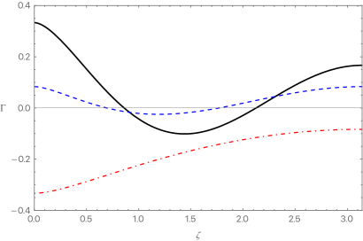
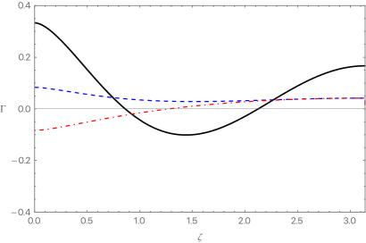
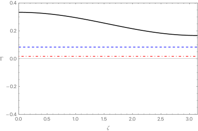
It is not straightforward to represent in a plot the rich, multi-parameter dependence of the response functions on the geometrical configuration of the system. For definiteness, in Fig 1, left panel, we represent the pulsar angular response to the kinematic dipole, both for intensity and circular polarization, as a function of the angle between pulsar directions. In the right panel, we represent the response functions to the kinematic quadrupole. We plot only the quantities between round parenthesis in eqs (3.12) and (3.14), without the geometrical factors depending on the relative velocity among frames. A more detailed analysis of the geometrical dependence on the various quantities is postponed to section 5. For the moment, it is sufficient to notice that the dependence on the pulsar separation of the functions and is qualitatively different from the Hellings-Downs curve, which we also represent for comparison.
3.3 Examples of SGWB frequency dependence
Besides the geometrical dependence of the results on the location of pulsars, the PTA response to Doppler effects depends on the frequency dependence of the isotropic part of the SGWB. In fact, the size and observational impact of kinematic anisotropies can be enhanced if the SGWB is characterised by large values for the slope parameters and of eqs (3.6), at least for certain ranges of frequencies. While current PTA data are compatible with a power-law profile of the isotropic SGWB as function of frequency, in the future more accurate data might favour other scenarios. For example, broken power law profiles, well motivated by a variety of SGWB sources [96], have also been considered in [1] for explaining the most recent pulsar timing array data (see also [97] for more complex profiles in frequency). The same is true for more complex SGWB profiles motivated by primordial black hole physics: see e.g. the first analysis carried out in [1, 98, 99, 100, 101] (and also [102] for a recent review on inflationary primordial black hole models).
We briefly outline the consequences of these two scenarios for the physics of kinematic anisotropies:
Broken power law: Consider the following broken power law Ansatz for the intensity profile [103, 104]
| (3.15) |
where we denote , and , , , are positive dimensionless parameters, while a pivot frequency within the PTA detection band. The associated tilt parameters result
| (3.16) |
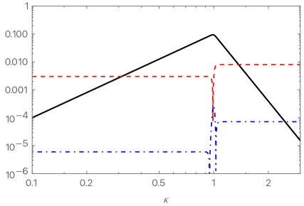
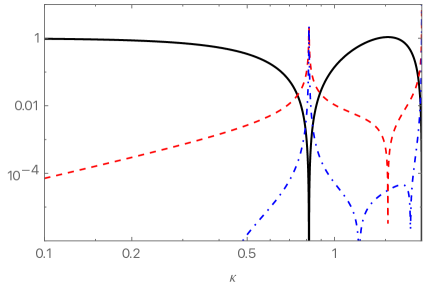
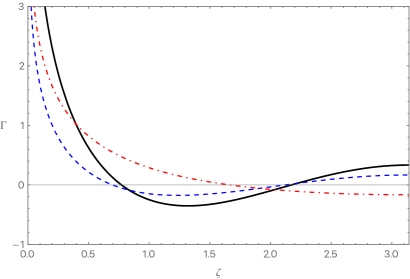
The resulting slope of the intensity spectrum is equal to the parameter at small frequencies, and to at larger frequencies. For a large values of , at intermediate frequencies the quantity can increase by several orders of magnitude, enhancing the quadrupolar kinematic anisotropies to a size comparable to the dipolar ones (see [105] for related effects explored for the case of interferometers). We represent in Fig 2, left panel, an example to visually demonstrate such behaviour for the slope parameters.
Second-order GW from primordial black hole formation: Primordial black holes can form in the early universe. Their formation requires to amplify the spectrum of scalar fluctuations for a range of scales around a pivot frequency , which we can consider in the PTA frequency ranges. At second order in perturbations, these mechanisms induce a SGWB, whose properties depend on the source scalar spectrum [106, 107, 108, 109] (see also [110, 111, 112]). For a narrow scalar spectrum whose width is much smaller than , we expect that the GW energy density increases as for small frequencies [113]. Then its profile has a dip (typically at scales around ), followed by a pronounced resonance. The frequency profile then drops its amplitude for (see the discussion in [108, 109]). Given that intensity is connected to the GW energy density through the relation , we can consider the following simple Ansatz for the intensity parameter (we call again )
| (3.17) |
as representative of the behaviour described above. In fact, the intensity is constant at small frequencies , for then developing the features described above. Hence, in this context,
| (3.18) | |||||
| (3.19) |
We represent in Fig 2, right panel, the resulting intensity and the slope parameter combinations characterizing kinematic anisotropies. In proximity of the dip in intensity which preceeds the resonance, the size of the slope parameters become so large that dipolar and quadrupolar anisotropies become comparable in size.
4 Kinematic anisotropies and modified gravity
Theories of gravity alternative to General Relativity allow for scalar and vector metric components to participate to gravitational interactions, and to contribute to the GW signal in terms of extra GW polarizations [114]. The PTA responses to scalar and vector polarizations have been derived in [85, 86, 87, 88, 89, 90, 91] for the case of isotropic backgrounds (see also the general treatment in [84]). Such extra polarizations induce correlations among pulsar signals distinct from the Hellings Downs curve. These alternative predictions are not favoured by recent detections [1], that can be used to set upper bounds on scalar and vector contributions to the isotropic backgrounds. Nevertheless, in view of future opportunities to further improve constraints (or maybe even detect signals of modified gravity), it is interesting to develop this topic, and analyse how scalar and vector GW polarizations contribute to kinematic anisotropies.
Analogously to the spin-2 case, the PTA response to kinematic anisotropies associated with extra GW polarisations are sensitive to the slope of scalar and vector spectra, as well as to the presence of parity violating effects in the vector sector. Doppler effects are unique probes of these features, which can increase the opportunities of detection. Here we derive for the first time analytical formulas describing the PTA response functions to kinematic anisotropies, associated with scalar and vector polarizations.
The procedure to follow for determining the PTA response to kinematic anisotropies is identical to what done in sections 2 and 3 for the tensor case – the only difference being that we utilize the corresponding scalar and vector GW polarization tensors, whose properties are described in Appendix A. In particular, the scalar and vector polarization tensors are used to perform angular integrals corresponding to eqs (2.15) and (2.16).
Scalar contributions to GW signal are characterized only by scalar intensity, and there is no circular polarization. We can assume that the total isotropic part for the intensity of the SGWB is made of a tensor and a scalar part, , possibly hierarchical in size as . We use the same notation of section 3. We introduce the slope parameters for each of the intensity contributions
| (4.1) | |||||
| (4.2) |
We find that the PTA response function to scalar part of the intensity is
| (4.3) |
where, beside the isotropic part, we consider the dipolar (proportional to ) and quadrupolar (proportional to ) kinematic anisotropy contributions. (Instead, the tensor part is identical to what discussed in section 3.) Interestingly – and differently from the tensor case – the PTA response to scalar kinematic anisotropies is independent from the angle among pulsars, while it depends on the angles among the pulsar directions and the frame velocity vector . See Fig 3, left panel. Moreover, it is proportional to , making it a unique probe of the slope of the scalar contribution to the total intensity (more on this in section 5).
Vector-tensor non-minimally coupled theories of gravity have also been introduced in view of applications to dark energy and black hole physics (see e.g. [115, 116, 117, 118]). The correlators among vector Fourier modes can be decomposed into intensity and circular polarization, analogously to what done in the tensor case in section 2. Using formulas (A.21) and (A.22), it is straightforward to compute the PTA response to dipolar anisotropies of the vector intensity and vector circular polarization, finding (the slope parameters are defined analogously as above)
The response to vector GW components does depend on the angular separation among pulsar directions. See Fig 3, right panel. It is very large for small angular separation among pulsars, where contributions of pulsar terms should nevertheless be included, see e.g. [85, 49]. In the second line of eq (LABEL:GammaVe1) we find in the first the pulsar dipolar response to vector intensity, that depends on the projection of the pulsar directions on the velocity vector . The second term controls the the pulsar dipolar response to vector circular polarization, depending on the projection of on a direction perpendicular to the plane of the two pulsar directions. These features are similar to what found for the spin-2 case, see section 3.
5 Strategies of detection
So far, we learned several interesting features of kinematic anisotropies, which make them potential probes of specific properties of the SGWB:
-
•
The geometrical configuration of the pulsar network enters in the PTA response functions, which depend in a distinctive way on intensity and circular polarization of the SGWB. While the response to GW intensity is maximal for pulsars whose positional vectors are in the direction of the Doppler velocity vector , the response to GW circular polarization is enhanced for pulsars lying on a plane orthogonal to . This distinct behaviour in the two cases can be used for selecting PTA sets aiming at distinguishing and independently measure the GW intensity and circular polarization.
-
•
The overall size of kinematic anisotropies can be amplified in scenarios with a rich frequency dependence of the isotropic part of the background, see e.g. section 3.3. This properties applies to GW backgrounds associated with standard spin-2 polarizations, but possibly also containing GW spin-0 and spin-1 contributions. Hence, a detection of kinematic anisotropies can give us a complementary probe of the slope of GW polarization components, which is difficult or even impossible to extract from the study of the isotropic part of the background only.
We now make concrete applications of our findings, in order to develop specific strategies of detection of different physical effects. In a sentence, the main feature we can exploit is the following:
-
The presence of kinematic anisotropies implies that signal correlations among pulsars do not follow the standard Hellings Downs angular distribution, but have deviations that depend on SGWB properties. Measurements of these deviations, that are deterministic and analytically calculable, can be used to extract information about the GW signal.
As explained in the Introduction, we are especially interested in using kinematic anisotropies as a probe of: 1. parity violation, 2. the frequency slope of correlation functions, 3. the presence of extra polarizations. We discuss these three topics in what follows.
5.1 Kinematic anisotropies and SGWB circular polarization
The effects of of parity violation in the SGWB kinematic anisotropies can be cleanly extracted from PTA data, once we make an appropriate choice of pulsars to monitor. In fact, it is not even necessary to make combinations among different signals, as proposed in the first work [80] discussing the topic (see also [81]). Choosing carefully the pulsar system, we can reduce sources of statistical errors by focussing only on pulsars located at convenient positions to reveal the presence of parity violation. Eqs (3.13) and (3.14) teach us that PTA are sensitive to circular polarization only through the anisotropies of the SGWB (as first pointed out in [80]), and moreover the corresponding signal is enhanced when maximising the quantity . (The same is true for parity violating effects in possible spin-1 polarization contributions, see section 4.)
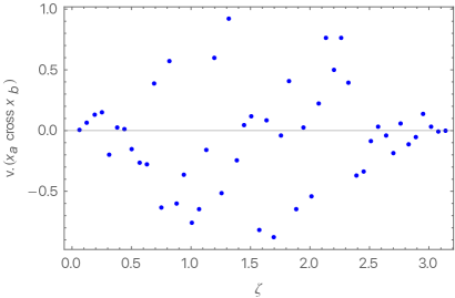
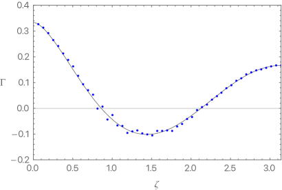
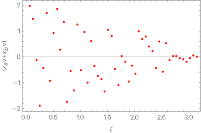
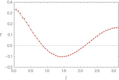
In Figure 4, left panel, we represent as a function of , for a random set of pulsar pairs whose positional vectors lie on a plane orthogonal with the velocity vector . The size of the quantity is maximal for intermediate values of , while it reduces at the extremes and . In the right panel of the figure we represent the response function to circular polarization, which shows that scattering effects are more pronounced for intermediate values of the angle .
Hence, to be maximally sensitive to circular polarization , it is convenient to focus on pulsars whose position vectors form a plane orthogonal to the direction of the velocity vector , so that we completely remove possible contaminations from kinematic effects due to GW intensity. The formula for the optimal signal-to-noise ratio for detecting the presence of in the PTA time-delay correlators is derived in Appendix B. It results
| (5.1) | |||||
where the sum is limited to pulsar pairs orthogonal to , as described above, and is the noise spectral density function (see Appendix B for more details). The general form for the circular polarization response is given in eq (3.13), and in the second line of eq (5.1) we write its contributions up to the dipole. Besides being proportional to , it also depends on the slope of the quantity , and might be enhanced if is a steep function of frequency. In fact, the study of kinematic anisotropies – given their unique dependence on the slope of the spectrum, see comments between eqs (3.7) and (3.8) – might represent the only way to probe the frequency-dependence of quantities associated with circular polarization. In the most conservative cases, in case with no pronounced features, in order to detect parity violating effects we would need a factor one thousand more in sensitivity with respect to current experiments.
5.2 Kinematic anisotropies and SGWB intensity
Suppose we are interested in extracting from the kinematic anisotropy contributions associated with the GW intensity as introduced in section 3.1. The corresponding response function of a pulsar pair to intensity Doppler effects is given by eq (3.9), which we rewrite here up to the dipole contributions:
| (5.2) |
Recall the definition of the parameter is expressed in terms of the angle between the unit vectors indicating the pulsar positions with respect to the Earth. The function (5.2) depends on through the first contribution between parenthesis, which corresponds to the Hellings Downs curve as defined in eq (3.10). But eq (5.2) also depends on the angle that each pulsar vector forms with the relative frame velocity . As explained in section 3, only pulsars whose vector components lie along are sensitive to kinematic anisotropies relative to the GW intensity.
When plotting the quantity as a function of for each pulsar pair in a given set, data points get scattered around the Hellings-Downs curve of eq (3.10) (see [48, 47]). In fact, data are modulated by the quantity in eq (5.2); we expect that point scattering around the Hellings-Downs line is maximal for small values of , while it reduces for , since in this limit the coefficient of the kinematic dipole contribution vanishes: . We represent in Fig 5, left panel, the value of the quantity as a function of , for a random set of pulsars whose positions are coplanar with the velocity vector . As anticipated, the size of this quantity reduces as we increase the angle . The right panel of the same figure shows the resulting response function as function of , which is indeed scattered for small angular separations with respect to the Hellings Downs curve. Hence, the effects of kinematic anisotropies relative to the GW intensity are maximal for pulsar pairs lying in the same plane as , and with whose positional vectors form a small relative angle among themselves. This represents an interesting difference with respect to the GW circular polarization response that we discussed in section 5.1.
As manifest from Fig 5, the kinematic effects we are interested in are small. On the other hand, by combining signals 666See the review [84] for a discussion of possibilities to combine GW signals to extract specific physical information from them., we can form null tests for Doppler effects associated to the intensity of the SGWB. To find such combinations, we further exploit the results of section 3. Suppose that GW are characterized by spin-2 polarization only, with no effects of parity violation. Then, consider two pairs of pulsars. One pair, , lies on a plane parallel to : hence it feels the effects of kinematic anisotropies, and the response function up to the dipole is given by eq (5.2). The other pair, , lies on a plane orthogonal to : hence it is blind to Doppler effects, and the pulsar response function is determined only by the Hellings Downs curve of eq (3.10).
We then take the following combination of equal-time correlators for time residuals (recall their definition in eq (2.14)):
| (5.3) |
where is the Hellings Downs function of eq (3.10), while is given in eq (3.11). Hence, in the context we are considering, a measurement of the combination (5.3) allows us to extract only the effects of kinematic anisotropies, with no contaminations from the isotropic background. Interestingly, given the dependence on the intensity slope in the numerator of eq (5.3), the sensitivity to kinematic anisotropies get enhanced for signals with features, see for example section 3.3. In this sense, kinematic anisotropies allow us to probe features in the frequency dependence of GW correlators.
While so far we discussed the dipole only, similar considerations hold for the quadrupole contributions, that as we have seen can be enhanced in scenarios with features in the isotropic SGWB as function of frequency. See Fig 6 for representative examples of kinematic quadrupole effects.
5.3 Kinematic anisotropies and scalar contributions to the GW signal
Models of modified gravity often predict the existence of light scalar fields associated with gravitational interactions. They contribute to GW as additional spin-0, scalar polarizations [114]. Scalars can contribute to the total GW intensity. But if their amplitude is well smaller than the tensor intensity amplitude , it might be hard to disentangle their contribution from analysing only the isotropic part of the background.
Interestingly, if the isotropic scalar intensity has a steep slope, or more generally it has pronounced features associated with its frequency dependence, its consequences on kinematic anisotropies can allow us to extract the presence of scalar polarization with PTA data.
In scenarios including contributions from the scalar polarization, we express the total GW intensity (tensor plus scalar parts) as
| (5.4) |
Defining the intensity slope parameters as in eqs (4.1), (4.2), we find that the PTA intensity response function to Doppler dipolar anisotropies in such scalar-tensor theories can be decomposed as
| (5.5) |
with
| (5.6) | |||||
| (5.7) |
The quantity describes the pulsar response to the isotropic part of the scalar-tensor intensity, while the pulsar response to the dipolar kinematic anisotropy. Hence, even if – so that is ‘almost blind’ to scalar contributions – a pronounced slope dependence, leading to can make sensitive to the scalar polarization. An appropriate combination of signals associated to different pulsar pairs, following the method described around eq (5.3), isolates the effects of scalar dipolar anisotropies in the response functions. Consequently, the presence of scalar polarizations might be detectable even if scalar polarizations contribute as small part to the GW signal amplitude.
6 Outlook
The recent detection of a stochastic gravitational wave background from several pulsar timing array collaborations opens a new window for gravitational wave cosmology. If the stochastic gravitational wave background has a cosmological origin, one of its guaranteed features are kinematic anisotropies due to our motion with respect to the gravitational wave source. In this work, we investigated the physical information that can be extracted from a detection of kinematic anisotropies. We shown that the pulsar response functions to Doppler effects depend on the stochastic background source and on the underlying gravitational physics. Furthermore, we stressed for the first time how the measured gravitational wave signal depends on the pulsar location with respect to the relative velocity among frames. We presented our results in a convenient way that emphasizes the geometrical dependence of the pulsar response functions to different properties of the stochastic background.
Our findings can be useful in planning future measurements, or in elaborating existing data, for using kinematic anisotropies to detect, or set more stringent constraints, on parity violation in gravitational interactions, on the presence of scalar/vector polarizations, or to develop independent probes of the frequency profile of the stochastic background. Besides backgrounds detectable at nano-Hertz frequencies with pulsar timing arrays, it would be interesting to apply our findings also to astrometric measurements of gravitational waves based on Gaia data, see e.g. the discussion in [119, 120, 121, 122, 123].
Current measurements (see [65]) set upper bounds on the amplitude of multipoles of the SGWB. The work [90] estimates that a detection is possible only for anisotropies whose size is of the order of 0.1 with respect to the isotropic background, unless the amplitude of the latter is measured with high SNR. However, the recent first detection of the isotropic part of the background by various international PTA collaborations gives hope for the future. Future measurements of pulsar timing residuals, for example by the SKA collaboration, will monitor many more pulsars than current experiments. Their higher sensitivity will improve the confidence on the detection of the isotropic part of the SGWB and its SNR, enhancing the opportunity to detect SGWB anisotropies.
The theoretical study in this manuscript adds further ingredients that can help in planning future dedicated searches of Doppler anisotropies. Moreover, the manuscript studies the consequences of SGWB with a frequency dependence that goes beyond a power law, as motivated for example by early universe models producing primordial black holes (see section 3.3). In this case, we cannot apply the factorizable Ansatz for the anisotropic SGWB often used in the literature, as constituted of a part depending on frequency, times a part depending on direction. In fact, we find that a SGWB with enhanced features in its frequency dependence can amplify the size of kinematic anisotropies to values well larger than the amplitude one would expect for kinematic anisotropies.
In our work, we assumed that the direction and amplitude of the velocity vector among the cosmological source of gravitational waves and the solar sytem baricenter coincides to what measured by the cosmic microwave background dipole. On the other hand, our formulas can be used to directly test this hypothesis, somehow analogously to the proposal [124] in the different context of radio sources. In fact, the topic of radio galaxy and quasar measurements of the cosmic dipole is a point of debate in recent literature [125, 126, 127, 128, 129, 130]. It would be interesting to use gravitational waves as an independent probe of the direction of the kinematic dipole, and test alternative scenarios based on large scale superhorizon isocurvature fluctuations [131, 132], intrinsic anisotropies [133], or more general deviations from the cosmological principle [134]. In this sense, this program belongs to the ‘multimessenger cosmology’ framework advocated in [135, 136].
Acknowledgments
It is a pleasure to thank Debika Chowdhury, Ameek Malhotra (especially), Maria Mylova, and Ivonne Zavala for useful input. GT is partially funded by the STFC grant ST/T000813/1. For the purpose of open access, the author has applied a Creative Commons Attribution licence to any Author Accepted Manuscript version arising.
Appendix A Identities involving the polarization tensors
We derive useful identities involving the polarization tensors entering in the Fourier transform of the GW signals, which we used in sections 2-4. We start discussing the spin-2 case, to then consider respectively the spin-0 and spin-1 cases.
Spin-2 polarization tensors: In the main text, section 3, we focussed on the basis for the polarization tensors. To develop our arguments, in this Appendix it is convenient to introduce the circular basis:
| (A.1) |
We assume that the polarization tensors are real quantities: hence . Notice also the identity
| (A.2) |
We identify the circular polarization indexes with : . The polarization tensors in the circular basis can be conveniently expressed as a product of polarization vectors:
| (A.3) |
The real unit vectors , are orthogonal among themselves and to the GW direction . We can express as
| (A.4) |
with the Levi-Civita tensor in three dimensions. (For what comes next, we do not need to make any specific choice for the direction .) It is easy to verify the following identity involving symmetric tensors
| (A.5) |
In fact, both the LHS and RHS are parallel to and , orthogonal to , and of trace 2. Moreover, the antisymmetric combination is orthogonal to , and satisfy the identity
| (A.6) |
We can convince ourselves of the validity of relation (A.6) by contracting with , :
| (A.7) |
and
| (A.8) |
Identities (A.5) and (A.6) ensure the relation (no summation over polarization indexes)
| (A.9) | |||||
| (A.10) | |||||
| (A.11) |
Hence:
| (A.12) | |||||
| (A.13) |
Expanding the product, and passing from the circular polarization to the original polarization using eq (A.2), we find the identities:
| (A.14) | |||||
and
| (A.15) |
We used these relations in the main text to obtain eqs (2.17) and (2.18), controlling the PTA response respectively to GW intensity and circular polarization.
Spin-0 polarization tensor: We can be brief here, since the spin-0 mode is associated with a single polarization tensor
| (A.16) |
which we used for deriving equation (4.3) in the main text.
Spin-1 polarization tensors: To describe spin-1 polarization tensors we can use a basis or a circular basis: they are related exactly as in eq (A.1) for the spin-2 case. In the circular basis , the vector polarization tensors read
| (A.17) |
with the vectors appearing in eq (A.3). We have the relation
| (A.20) |
Proceeding as we did in deriving eqs (A.14) and (A.15) for the spin-2 case, we can then obtain the following identities for vector polarizations in the basis:
| (A.21) |
and
| (A.22) |
that we used for deriving equation (LABEL:GammaVe1) in the main text.
Appendix B The optimal signal-to-noise ratio
In this Appendix we discuss the computation of the signal-to-noise ratio, in terms of a match-filtering technique as discussed in the paper [46] and the textbook [137]. We focus here on the case of spin-2 polarizations, but the arguments are the same for spin-1 and spin-0. We assume that the noise dominates over the signal. The latter can be extracted once we know its properties.
The stationary two-point correlator for time-delays of pulsar measurements summed over a PTA set of pulsar pairs is weighted by an appropriate choice of filters
| (B.1) |
where indicates the duration of the experiment. We pass to Fourier space, and write the previous expression as
| (B.2) |
The ‘finite-time’ delta-function is
| (B.3) |
We assume that is real, and its Fourier transform obeys . Decomposed in real and imaginary part, we can express it as
| (B.4) |
with two real functions of frequency. In defining the SNR, the signal is the averaged value of when the GW signal is present; the noise is root mean square of when the GW is absent. The aim is to determine the optimal filter functions and for extracting the GW signal from the noise.
We start expressing the signal , as
| (B.5) |
Using formulas developed in section 2, we can write the two-point correlator in Fourier space as
| (B.6) | |||||
| (B.7) |
We plug this expression in eq (B.5), and use the decomposition (B.4), finding
| (B.8) |
since . The computation of the noise is identical to the textbook treatment of [137]. Characterizing the correlator of pulsar noise in terms of the quantity as
| (B.9) |
the square of the noise is
| (B.10) |
Hence, the signal-to-noise ratio results
| (B.11) |
We now determine the optimal choice of filter function that maximises the SNR. Given a tensor with structure
| (B.12) |
where the dots run over the pulsar pairs, one considers the positive-definite product
| (B.13) |
Using this tool, we can schematically express the SNR of eq (B.11) as
| (B.14) |
We now have different options:
-
•
If we wish to maximise the SNR to the total signal (intensity and circular polarization combined) we choose the filter which obviously maximises the scalar product of eq (B.14). Using this filter we conclude that the optimal SNR is
(B.15) Its value depends on the GW intensity and circular polarization, and on the geometric quantities constituting and , as discussed in the main text.
-
•
We can instead be interested to extract from the signal only components associated for example to circular polarization, and determine the filter better suited to this purpose. The filter is then (i.e. a filter whose Fourier transform has only imaginary and no real component), and the associated SNR is
(B.16) As discussed in the main text, the sensitivity to circular polarization is then enhanced by selecting pulsars whose directions form a plane orthogonal to the velocity vector between SGWB source and detector frames.
-
•
Analogously, if we wish only to be sensitive to the GW intensity, we select a filter with real part only, and the maximal SNR is
(B.17) The sensitivity to intensity is enhanced by selecting pulsars whose directions are parallel to the velocity vector between SGWB source and detector frames.
References
- [1] NANOGrav Collaboration, G. Agazie et al., “The NANOGrav 15 yr Data Set: Evidence for a Gravitational-wave Background,” Astrophys. J. Lett. 951 no. 1, (2023) L8, arXiv:2306.16213 [astro-ph.HE].
- [2] D. J. Reardon et al., “Search for an Isotropic Gravitational-wave Background with the Parkes Pulsar Timing Array,” Astrophys. J. Lett. 951 no. 1, (2023) L6, arXiv:2306.16215 [astro-ph.HE].
- [3] EPTA Collaboration, J. Antoniadis et al., “The second data release from the European Pulsar Timing Array III. Search for gravitational wave signals,” arXiv:2306.16214 [astro-ph.HE].
- [4] H. Xu et al., “Searching for the Nano-Hertz Stochastic Gravitational Wave Background with the Chinese Pulsar Timing Array Data Release I,” Res. Astron. Astrophys. 23 no. 7, (2023) 075024, arXiv:2306.16216 [astro-ph.HE].
- [5] J. Ellis, M. Fairbairn, G. Franciolini, G. Hütsi, A. Iovino, M. Lewicki, M. Raidal, J. Urrutia, V. Vaskonen, and H. Veermäe, “What is the source of the PTA GW signal?,” arXiv:2308.08546 [astro-ph.CO].
- [6] R. Jackiw and S. Y. Pi, “Chern-Simons modification of general relativity,” Phys. Rev. D 68 (2003) 104012, arXiv:gr-qc/0308071.
- [7] S. H.-S. Alexander, M. E. Peskin, and M. M. Sheikh-Jabbari, “Leptogenesis from gravity waves in models of inflation,” Phys. Rev. Lett. 96 (2006) 081301, arXiv:hep-th/0403069.
- [8] A. Lue, L.-M. Wang, and M. Kamionkowski, “Cosmological signature of new parity violating interactions,” Phys. Rev. Lett. 83 (1999) 1506–1509, arXiv:astro-ph/9812088.
- [9] M. Satoh, S. Kanno, and J. Soda, “Circular Polarization of Primordial Gravitational Waves in String-inspired Inflationary Cosmology,” Phys. Rev. D 77 (2008) 023526, arXiv:0706.3585 [astro-ph].
- [10] C. R. Contaldi, J. Magueijo, and L. Smolin, “Anomalous CMB polarization and gravitational chirality,” Phys. Rev. Lett. 101 (2008) 141101, arXiv:0806.3082 [astro-ph].
- [11] M. M. Anber and L. Sorbo, “Naturally inflating on steep potentials through electromagnetic dissipation,” Phys. Rev. D 81 (2010) 043534, arXiv:0908.4089 [hep-th].
- [12] S. Alexander and N. Yunes, “Chern-Simons Modified General Relativity,” Phys. Rept. 480 (2009) 1–55, arXiv:0907.2562 [hep-th].
- [13] T. Takahashi and J. Soda, “Chiral Primordial Gravitational Waves from a Lifshitz Point,” Phys. Rev. Lett. 102 (2009) 231301, arXiv:0904.0554 [hep-th].
- [14] M. M. Anber and L. Sorbo, “Non-Gaussianities and chiral gravitational waves in natural steep inflation,” Phys. Rev. D 85 (2012) 123537, arXiv:1203.5849 [astro-ph.CO].
- [15] N. Bartolo et al., “Science with the space-based interferometer LISA. IV: Probing inflation with gravitational waves,” JCAP 12 (2016) 026, arXiv:1610.06481 [astro-ph.CO].
- [16] M. Mylova, “Chiral primordial gravitational waves in extended theories of Scalar-Tensor gravity,” arXiv:1912.00800 [gr-qc].
- [17] O. Özsoy, “Parity violating non-Gaussianity from axion-gauge field dynamics,” Phys. Rev. D 104 no. 12, (2021) 123523, arXiv:2106.14895 [astro-ph.CO].
- [18] C. Fu, J. Liu, X.-Y. Yang, W.-W. Yu, and Y. Zhang, “Explaining Pulsar Timing Array Observations with Primordial Gravitational Waves in Parity-Violating Gravity,” arXiv:2308.15329 [astro-ph.CO].
- [19] N. Bartolo, V. Domcke, D. G. Figueroa, J. García-Bellido, M. Peloso, M. Pieroni, A. Ricciardone, M. Sakellariadou, L. Sorbo, and G. Tasinato, “Probing non-Gaussian Stochastic Gravitational Wave Backgrounds with LISA,” JCAP 11 (2018) 034, arXiv:1806.02819 [astro-ph.CO].
- [20] N. Bartolo, V. De Luca, G. Franciolini, A. Lewis, M. Peloso, and A. Riotto, “Primordial Black Hole Dark Matter: LISA Serendipity,” Phys. Rev. Lett. 122 no. 21, (2019) 211301, arXiv:1810.12218 [astro-ph.CO].
- [21] C. Powell and G. Tasinato, “Probing a stationary non-Gaussian background of stochastic gravitational waves with pulsar timing arrays,” JCAP 01 (2020) 017, arXiv:1910.04758 [gr-qc].
- [22] G. Tasinato, “Gravitational wave nonlinearities and pulsar-timing array angular correlations,” Phys. Rev. D 105 no. 8, (2022) 083506, arXiv:2203.15440 [gr-qc].
- [23] LISA Cosmology Working Group Collaboration, N. Bartolo et al., “Probing anisotropies of the Stochastic Gravitational Wave Background with LISA,” JCAP 11 (2022) 009, arXiv:2201.08782 [astro-ph.CO].
- [24] G. F. Smoot, M. V. Gorenstein, and R. A. Muller, “Detection of Anisotropy in the Cosmic Black Body Radiation,” Phys. Rev. Lett. 39 (1977) 898.
- [25] A. Kogut et al., “Dipole anisotropy in the COBE DMR first year sky maps,” Astrophys. J. 419 (1993) 1, arXiv:astro-ph/9312056.
- [26] WMAP Collaboration, C. L. Bennett et al., “First year Wilkinson Microwave Anisotropy Probe (WMAP) observations: Preliminary maps and basic results,” Astrophys. J. Suppl. 148 (2003) 1–27, arXiv:astro-ph/0302207.
- [27] Planck Collaboration, N. Aghanim et al., “Planck 2013 results. XXVII. Doppler boosting of the CMB: Eppur si muove,” Astron. Astrophys. 571 (2014) A27, arXiv:1303.5087 [astro-ph.CO].
- [28] N. J. Cornish and A. Sesana, “Pulsar Timing Array Analysis for Black Hole Backgrounds,” Class. Quant. Grav. 30 (2013) 224005, arXiv:1305.0326 [gr-qc].
- [29] N. J. Cornish and L. Sampson, “Towards Robust Gravitational Wave Detection with Pulsar Timing Arrays,” Phys. Rev. D 93 no. 10, (2016) 104047, arXiv:1512.06829 [gr-qc].
- [30] S. R. Taylor, R. van Haasteren, and A. Sesana, “From Bright Binaries To Bumpy Backgrounds: Mapping Realistic Gravitational Wave Skies With Pulsar-Timing Arrays,” Phys. Rev. D 102 no. 8, (2020) 084039, arXiv:2006.04810 [astro-ph.IM].
- [31] B. Bécsy, N. J. Cornish, and L. Z. Kelley, “Exploring Realistic Nanohertz Gravitational-wave Backgrounds,” Astrophys. J. 941 no. 2, (2022) 119, arXiv:2207.01607 [astro-ph.HE].
- [32] B. Allen, “Variance of the Hellings-Downs correlation,” Phys. Rev. D 107 no. 4, (2023) 043018, arXiv:2205.05637 [gr-qc].
- [33] G. Sato-Polito and M. Kamionkowski, “Pulsar-timing measurement of the circular polarization of the stochastic gravitational-wave background,” Phys. Rev. D 106 no. 2, (2022) 023004, arXiv:2111.05867 [astro-ph.CO].
- [34] V. Alba and J. Maldacena, “Primordial gravity wave background anisotropies,” JHEP 03 (2016) 115, arXiv:1512.01531 [hep-th].
- [35] C. R. Contaldi, “Anisotropies of Gravitational Wave Backgrounds: A Line Of Sight Approach,” Phys. Lett. B 771 (2017) 9–12, arXiv:1609.08168 [astro-ph.CO].
- [36] M. Geller, A. Hook, R. Sundrum, and Y. Tsai, “Primordial Anisotropies in the Gravitational Wave Background from Cosmological Phase Transitions,” Phys. Rev. Lett. 121 no. 20, (2018) 201303, arXiv:1803.10780 [hep-ph].
- [37] N. Bartolo, D. Bertacca, S. Matarrese, M. Peloso, A. Ricciardone, A. Riotto, and G. Tasinato, “Anisotropies and non-Gaussianity of the Cosmological Gravitational Wave Background,” Phys. Rev. D 100 no. 12, (2019) 121501, arXiv:1908.00527 [astro-ph.CO].
- [38] N. Bartolo, D. Bertacca, V. De Luca, G. Franciolini, S. Matarrese, M. Peloso, A. Ricciardone, A. Riotto, and G. Tasinato, “Gravitational wave anisotropies from primordial black holes,” JCAP 02 (2020) 028, arXiv:1909.12619 [astro-ph.CO].
- [39] N. Bartolo, D. Bertacca, S. Matarrese, M. Peloso, A. Ricciardone, A. Riotto, and G. Tasinato, “Characterizing the cosmological gravitational wave background: Anisotropies and non-Gaussianity,” Phys. Rev. D 102 no. 2, (2020) 023527, arXiv:1912.09433 [astro-ph.CO].
- [40] E. Dimastrogiovanni, M. Fasiello, A. Malhotra, P. D. Meerburg, and G. Orlando, “Testing the early universe with anisotropies of the gravitational wave background,” JCAP 02 no. 02, (2022) 040, arXiv:2109.03077 [astro-ph.CO].
- [41] G. Cusin and G. Tasinato, “Doppler boosting the stochastic gravitational wave background,” JCAP 08 no. 08, (2022) 036, arXiv:2201.10464 [astro-ph.CO].
- [42] D. Bertacca, A. Ricciardone, N. Bellomo, A. C. Jenkins, S. Matarrese, A. Raccanelli, T. Regimbau, and M. Sakellariadou, “Projection effects on the observed angular spectrum of the astrophysical stochastic gravitational wave background,” Phys. Rev. D 101 no. 10, (2020) 103513, arXiv:1909.11627 [astro-ph.CO].
- [43] L. Valbusa Dall’Armi, A. Ricciardone, and D. Bertacca, “The dipole of the astrophysical gravitational-wave background,” JCAP 11 (2022) 040, arXiv:2206.02747 [astro-ph.CO].
- [44] A. K.-W. Chung, A. C. Jenkins, J. D. Romano, and M. Sakellariadou, “Targeted search for the kinematic dipole of the gravitational-wave background,” Phys. Rev. D 106 no. 8, (2022) 082005, arXiv:2208.01330 [gr-qc].
- [45] D. Chowdhury, G. Tasinato, and I. Zavala, “Response of the Einstein Telescope to Doppler anisotropies,” Phys. Rev. D 107 no. 8, (2023) 083516, arXiv:2209.05770 [gr-qc].
- [46] M. Anholm, S. Ballmer, J. D. E. Creighton, L. R. Price, and X. Siemens, “Optimal strategies for gravitational wave stochastic background searches in pulsar timing data,” Phys. Rev. D 79 (2009) 084030, arXiv:0809.0701 [gr-qc].
- [47] C. M. F. Mingarelli, T. Sidery, I. Mandel, and A. Vecchio, “Characterizing gravitational wave stochastic background anisotropy with pulsar timing arrays,” Phys. Rev. D 88 no. 6, (2013) 062005, arXiv:1306.5394 [astro-ph.HE].
- [48] S. R. Taylor and J. R. Gair, “Searching For Anisotropic Gravitational-wave Backgrounds Using Pulsar Timing Arrays,” Phys. Rev. D 88 (2013) 084001, arXiv:1306.5395 [gr-qc].
- [49] J. Gair, J. D. Romano, S. Taylor, and C. M. F. Mingarelli, “Mapping gravitational-wave backgrounds using methods from CMB analysis: Application to pulsar timing arrays,” Phys. Rev. D 90 no. 8, (2014) 082001, arXiv:1406.4664 [gr-qc].
- [50] N. J. Cornish and R. van Haasteren, “Mapping the nano-Hertz gravitational wave sky,” arXiv:1406.4511 [gr-qc].
- [51] C. M. F. Mingarelli, T. J. W. Lazio, A. Sesana, J. E. Greene, J. A. Ellis, C.-P. Ma, S. Croft, S. Burke-Spolaor, and S. R. Taylor, “The Local Nanohertz Gravitational-Wave Landscape From Supermassive Black Hole Binaries,” Nature Astron. 1 no. 12, (2017) 886–892, arXiv:1708.03491 [astro-ph.GA].
- [52] Y. Ali-Haïmoud, T. L. Smith, and C. M. F. Mingarelli, “Fisher formalism for anisotropic gravitational-wave background searches with pulsar timing arrays,” Phys. Rev. D 102 no. 12, (2020) 122005, arXiv:2006.14570 [gr-qc].
- [53] Y. Ali-Haïmoud, T. L. Smith, and C. M. F. Mingarelli, “Insights into searches for anisotropies in the nanohertz gravitational-wave background,” Phys. Rev. D 103 no. 4, (2021) 042009, arXiv:2010.13958 [gr-qc].
- [54] B. Allen and A. C. Ottewill, “Detection of anisotropies in the gravitational wave stochastic background,” Phys. Rev. D56 (1997) 545–563, arXiv:gr-qc/9607068 [gr-qc].
- [55] S. W. Ballmer, “A Radiometer for stochastic gravitational waves,” Class. Quant. Grav. 23 (2006) S179–S186, arXiv:gr-qc/0510096.
- [56] E. Thrane, S. Ballmer, J. D. Romano, S. Mitra, D. Talukder, S. Bose, and V. Mandic, “Probing the anisotropies of a stochastic gravitational-wave background using a network of ground-based laser interferometers,” Phys. Rev. D 80 (2009) 122002, arXiv:0910.0858 [astro-ph.IM].
- [57] A. I. Renzini and C. R. Contaldi, “Mapping Incoherent Gravitational Wave Backgrounds,” Mon. Not. Roy. Astron. Soc. 481 no. 4, (2018) 4650–4661, arXiv:1806.11360 [astro-ph.IM].
- [58] E. Payne, S. Banagiri, P. Lasky, and E. Thrane, “Searching for anisotropy in the distribution of binary black hole mergers,” Phys. Rev. D 102 no. 10, (2020) 102004, arXiv:2006.11957 [astro-ph.CO].
- [59] N. J. Cornish, “Mapping the gravitational wave background,” Class. Quant. Grav. 18 (2001) 4277–4292, arXiv:astro-ph/0105374.
- [60] J. Baker et al., “High angular resolution gravitational wave astronomy,” Exper. Astron. 51 no. 3, (2021) 1441–1470, arXiv:1908.11410 [astro-ph.HE].
- [61] S. Banagiri, A. Criswell, T. Kuan, V. Mandic, J. D. Romano, and S. R. Taylor, “Mapping the gravitational-wave sky with LISA: a Bayesian spherical harmonic approach,” Mon. Not. Roy. Astron. Soc. 507 no. 4, (2021) 5451–5462, arXiv:2103.00826 [astro-ph.IM].
- [62] C. R. Contaldi, M. Pieroni, A. I. Renzini, G. Cusin, N. Karnesis, M. Peloso, A. Ricciardone, and G. Tasinato, “Maximum likelihood map-making with the Laser Interferometer Space Antenna,” Phys. Rev. D 102 no. 4, (2020) 043502, arXiv:2006.03313 [astro-ph.CO].
- [63] LISA Cosmology Working Group Collaboration, P. Auclair et al., “Cosmology with the Laser Interferometer Space Antenna,” arXiv:2204.05434 [astro-ph.CO].
- [64] S. R. Taylor et al., “Limits on anisotropy in the nanohertz stochastic gravitational-wave background,” Phys. Rev. Lett. 115 no. 4, (2015) 041101, arXiv:1506.08817 [astro-ph.HE].
- [65] NANOGrav Collaboration, G. Agazie et al., “The NANOGrav 15-year Data Set: Search for Anisotropy in the Gravitational-Wave Background,” arXiv:2306.16221 [astro-ph.HE].
- [66] Y.-K. Chu, G.-C. Liu, and K.-W. Ng, “Observation of a polarized stochastic gravitational-wave background in pulsar-timing-array experiments,” Phys. Rev. D 104 no. 12, (2021) 124018, arXiv:2107.00536 [gr-qc].
- [67] R. C. Bernardo and K.-W. Ng, “Stochastic gravitational wave background phenomenology in a pulsar timing array,” Phys. Rev. D 107 no. 4, (2023) 044007, arXiv:2208.12538 [gr-qc].
- [68] R. C. Bernardo and K.-W. Ng, “Constraining gravitational wave propagation using pulsar timing array correlations,” Phys. Rev. D 107 no. 10, (2023) L101502, arXiv:2302.11796 [gr-qc].
- [69] M. Branchesi et al., “Science with the Einstein Telescope: a comparison of different designs,” JCAP 07 (2023) 068, arXiv:2303.15923 [gr-qc].
- [70] E. F. Keane et al., “A Cosmic Census of Radio Pulsars with the SKA,” PoS AASKA14 (2015) 040, arXiv:1501.00056 [astro-ph.IM].
- [71] G. Janssen et al., “Gravitational wave astronomy with the SKA,” PoS AASKA14 (2015) 037, arXiv:1501.00127 [astro-ph.IM].
- [72] T. L. Smith and R. Caldwell, “Sensitivity to a Frequency-Dependent Circular Polarization in an Isotropic Stochastic Gravitational Wave Background,” Phys. Rev. D 95 no. 4, (2017) 044036, arXiv:1609.05901 [gr-qc].
- [73] S. G. Crowder, R. Namba, V. Mandic, S. Mukohyama, and M. Peloso, “Measurement of Parity Violation in the Early Universe using Gravitational-wave Detectors,” Phys. Lett. B 726 (2013) 66–71, arXiv:1212.4165 [astro-ph.CO].
- [74] N. Seto, “Gravitational Wave Background Search by Correlating Multiple Triangular Detectors in the mHz Band,” Phys. Rev. D 102 no. 12, (2020) 123547, arXiv:2010.06877 [gr-qc].
- [75] G. Orlando, M. Pieroni, and A. Ricciardone, “Measuring Parity Violation in the Stochastic Gravitational Wave Background with the LISA-Taiji network,” JCAP 03 (2021) 069, arXiv:2011.07059 [astro-ph.CO].
- [76] N. Seto and A. Taruya, “Polarization analysis of gravitational-wave backgrounds from the correlation signals of ground-based interferometers: Measuring a circular-polarization mode,” Phys. Rev. D 77 (2008) 103001, arXiv:0801.4185 [astro-ph].
- [77] N. Seto, “Prospects for direct detection of circular polarization of gravitational-wave background,” Phys. Rev. Lett. 97 (2006) 151101, arXiv:astro-ph/0609504.
- [78] N. Seto, “Quest for circular polarization of gravitational wave background and orbits of laser interferometers in space,” Phys. Rev. D 75 (2007) 061302, arXiv:astro-ph/0609633.
- [79] V. Domcke, J. Garcia-Bellido, M. Peloso, M. Pieroni, A. Ricciardone, L. Sorbo, and G. Tasinato, “Measuring the net circular polarization of the stochastic gravitational wave background with interferometers,” JCAP 05 (2020) 028, arXiv:1910.08052 [astro-ph.CO].
- [80] R. Kato and J. Soda, “Probing circular polarization in stochastic gravitational wave background with pulsar timing arrays,” Phys. Rev. D 93 no. 6, (2016) 062003, arXiv:1512.09139 [gr-qc].
- [81] E. Belgacem and M. Kamionkowski, “Chirality of the gravitational-wave background and pulsar-timing arrays,” Phys. Rev. D 102 no. 2, (2020) 023004, arXiv:2004.05480 [astro-ph.CO].
- [82] C. Caprini, D. G. Figueroa, R. Flauger, G. Nardini, M. Peloso, M. Pieroni, A. Ricciardone, and G. Tasinato, “Reconstructing the spectral shape of a stochastic gravitational wave background with LISA,” JCAP 11 (2019) 017, arXiv:1906.09244 [astro-ph.CO].
- [83] A. Nishizawa, A. Taruya, K. Hayama, S. Kawamura, and M.-a. Sakagami, “Probing non-tensorial polarizations of stochastic gravitational-wave backgrounds with ground-based laser interferometers,” Phys. Rev. D 79 (2009) 082002, arXiv:0903.0528 [astro-ph.CO].
- [84] J. D. Romano and N. J. Cornish, “Detection methods for stochastic gravitational-wave backgrounds: a unified treatment,” Living Rev. Rel. 20 no. 1, (2017) 2, arXiv:1608.06889 [gr-qc].
- [85] K. J. Lee, F. A. Jenet, and R. H. Price, “Pulsar timing as a probe of non-einsteinian polarizations of gravitational waves,” The Astrophysical Journal 685 no. 2, (Oct, 2008) 1304. https://dx.doi.org/10.1086/591080.
- [86] J. R. Gair, M. Vallisneri, S. L. Larson, and J. G. Baker, “Testing General Relativity with Low-Frequency, Space-Based Gravitational-Wave Detectors,” Living Rev. Rel. 16 (2013) 7, arXiv:1212.5575 [gr-qc].
- [87] S. J. Chamberlin and X. Siemens, “Stochastic backgrounds in alternative theories of gravity: overlap reduction functions for pulsar timing arrays,” Phys. Rev. D 85 (2012) 082001, arXiv:1111.5661 [astro-ph.HE].
- [88] L. Shao et al., “Testing Gravity with Pulsars in the SKA Era,” PoS AASKA14 (2015) 042, arXiv:1501.00058 [astro-ph.HE].
- [89] J. R. Gair, J. D. Romano, and S. R. Taylor, “Mapping gravitational-wave backgrounds of arbitrary polarisation using pulsar timing arrays,” Phys. Rev. D 92 no. 10, (2015) 102003, arXiv:1506.08668 [gr-qc].
- [90] S. C. Hotinli, M. Kamionkowski, and A. H. Jaffe, “The search for anisotropy in the gravitational-wave background with pulsar-timing arrays,” Open J. Astrophys. 2 no. 1, (2019) 8, arXiv:1904.05348 [astro-ph.CO].
- [91] G.-C. Liu and K.-W. Ng, “Timing-residual power spectrum of a polarized stochastic gravitational-wave background in pulsar-timing-array observation,” Phys. Rev. D 106 no. 6, (2022) 064004, arXiv:2201.06767 [gr-qc].
- [92] M. Maggiore, Gravitational Waves. Vol. 2: Astrophysics and Cosmology. Oxford University Press, 3, 2018.
- [93] J. D. Romano and B. Allen, “Answers to frequently asked questions about the pulsar timing array Hellings and Downs correlation curve,” arXiv:2308.05847 [gr-qc].
- [94] R. w. Hellings and G. s. Downs, “UPPER LIMITS ON THE ISOTROPIC GRAVITATIONAL RADIATION BACKGROUND FROM PULSAR TIMING ANALYSIS,” Astrophys. J. Lett. 265 (1983) L39–L42.
- [95] F. A. Jenet and J. D. Romano, “Understanding the gravitational-wave Hellings and Downs curve for pulsar timing arrays in terms of sound and electromagnetic waves,” Am. J. Phys. 83 (2015) 635, arXiv:1412.1142 [gr-qc].
- [96] S. Kuroyanagi, T. Chiba, and T. Takahashi, “Probing the Universe through the Stochastic Gravitational Wave Background,” JCAP 11 (2018) 038, arXiv:1807.00786 [astro-ph.CO].
- [97] G. Ye and A. Silvestri, “Can the gravitational wave background feel wiggles in spacetime?,” arXiv:2307.05455 [astro-ph.CO].
- [98] NANOGrav Collaboration, A. Afzal et al., “The NANOGrav 15 yr Data Set: Search for Signals from New Physics,” Astrophys. J. Lett. 951 no. 1, (2023) L11, arXiv:2306.16219 [astro-ph.HE].
- [99] EPTA Collaboration, J. Antoniadis et al., “The second data release from the European Pulsar Timing Array: V. Implications for massive black holes, dark matter and the early Universe,” arXiv:2306.16227 [astro-ph.CO].
- [100] G. Franciolini, A. Iovino, Junior., V. Vaskonen, and H. Veermae, “The recent gravitational wave observation by pulsar timing arrays and primordial black holes: the importance of non-gaussianities,” arXiv:2306.17149 [astro-ph.CO].
- [101] D. G. Figueroa, M. Pieroni, A. Ricciardone, and P. Simakachorn, “Cosmological Background Interpretation of Pulsar Timing Array Data,” arXiv:2307.02399 [astro-ph.CO].
- [102] O. Özsoy and G. Tasinato, “Inflation and Primordial Black Holes,” Universe 9 no. 5, (2023) 203, arXiv:2301.03600 [astro-ph.CO].
- [103] L. Sampson, N. J. Cornish, and S. T. McWilliams, “Constraining the Solution to the Last Parsec Problem with Pulsar Timing,” Phys. Rev. D 91 no. 8, (2015) 084055, arXiv:1503.02662 [gr-qc].
- [104] A. R. Kaiser, N. S. Pol, M. A. McLaughlin, S. Chen, J. S. Hazboun, L. Z. Kelley, J. Simon, S. R. Taylor, S. J. Vigeland, and C. A. Witt, “Disentangling Multiple Stochastic Gravitational Wave Background Sources in PTA Data Sets,” Astrophys. J. 938 no. 2, (2022) 115, arXiv:2208.02307 [astro-ph.CO].
- [105] E. Dimastrogiovanni, M. Fasiello, A. Malhotra, and G. Tasinato, “Enhancing gravitational wave anisotropies with peaked scalar sources,” JCAP 01 (2023) 018, arXiv:2205.05644 [astro-ph.CO].
- [106] K. N. Ananda, C. Clarkson, and D. Wands, “The Cosmological gravitational wave background from primordial density perturbations,” Phys. Rev. D 75 (2007) 123518, arXiv:gr-qc/0612013.
- [107] D. Baumann, P. J. Steinhardt, K. Takahashi, and K. Ichiki, “Gravitational Wave Spectrum Induced by Primordial Scalar Perturbations,” Phys. Rev. D 76 (2007) 084019, arXiv:hep-th/0703290.
- [108] R. Saito and J. Yokoyama, “Gravitational wave background as a probe of the primordial black hole abundance,” Phys. Rev. Lett. 102 (2009) 161101, arXiv:0812.4339 [astro-ph]. [Erratum: Phys.Rev.Lett. 107, 069901 (2011)].
- [109] R. Saito and J. Yokoyama, “Gravitational-Wave Constraints on the Abundance of Primordial Black Holes,” Prog. Theor. Phys. 123 (2010) 867–886, arXiv:0912.5317 [astro-ph.CO]. [Erratum: Prog.Theor.Phys. 126, 351–352 (2011)].
- [110] G. Domènech, “Induced gravitational waves in a general cosmological background,” Int. J. Mod. Phys. D 29 no. 03, (2020) 2050028, arXiv:1912.05583 [gr-qc].
- [111] G. Domènech, S. Pi, and M. Sasaki, “Induced gravitational waves as a probe of thermal history of the universe,” JCAP 08 (2020) 017, arXiv:2005.12314 [gr-qc].
- [112] G. Domènech, “Scalar Induced Gravitational Waves Review,” Universe 7 no. 11, (2021) 398, arXiv:2109.01398 [gr-qc].
- [113] R.-G. Cai, S. Pi, and M. Sasaki, “Universal infrared scaling of gravitational wave background spectra,” Phys. Rev. D 102 no. 8, (2020) 083528, arXiv:1909.13728 [astro-ph.CO].
- [114] D. M. Eardley, D. L. Lee, A. P. Lightman, R. V. Wagoner, and C. M. Will, “Gravitational-wave observations as a tool for testing relativistic gravity,” Phys. Rev. Lett. 30 (1973) 884–886.
- [115] G. Tasinato, “Cosmic Acceleration from Abelian Symmetry Breaking,” JHEP 04 (2014) 067, arXiv:1402.6450 [hep-th].
- [116] L. Heisenberg, “Generalization of the Proca Action,” JCAP 05 (2014) 015, arXiv:1402.7026 [hep-th].
- [117] G. Tasinato, “A small cosmological constant from Abelian symmetry breaking,” Class. Quant. Grav. 31 (2014) 225004, arXiv:1404.4883 [hep-th].
- [118] J. Chagoya, G. Niz, and G. Tasinato, “Black Holes and Abelian Symmetry Breaking,” Class. Quant. Grav. 33 no. 17, (2016) 175007, arXiv:1602.08697 [hep-th].
- [119] L. G. Book and E. E. Flanagan, “Astrometric Effects of a Stochastic Gravitational Wave Background,” Phys. Rev. D 83 (2011) 024024, arXiv:1009.4192 [astro-ph.CO].
- [120] C. J. Moore, D. P. Mihaylov, A. Lasenby, and G. Gilmore, “Astrometric Search Method for Individually Resolvable Gravitational Wave Sources with Gaia,” Phys. Rev. Lett. 119 no. 26, (2017) 261102, arXiv:1707.06239 [astro-ph.IM].
- [121] D. P. Mihaylov, C. J. Moore, J. R. Gair, A. Lasenby, and G. Gilmore, “Astrometric Effects of Gravitational Wave Backgrounds with non-Einsteinian Polarizations,” Phys. Rev. D 97 no. 12, (2018) 124058, arXiv:1804.00660 [gr-qc].
- [122] L. O’Beirne and N. J. Cornish, “Constraining the Polarization Content of Gravitational Waves with Astrometry,” Phys. Rev. D 98 no. 2, (2018) 024020, arXiv:1804.03146 [gr-qc].
- [123] W. Qin, K. K. Boddy, M. Kamionkowski, and L. Dai, “Pulsar-timing arrays, astrometry, and gravitational waves,” Phys. Rev. D 99 no. 6, (2019) 063002, arXiv:1810.02369 [astro-ph.CO].
- [124] G. F. R. Ellis and J. E. Baldwin, “On the expected anisotropy of radio source counts,” Monthly Notices of the Royal Astronomical Society 206 no. 2, (01, 1984) 377–381.
- [125] C. Blake and J. Wall, “Detection of the velocity dipole in the radio galaxies of the nrao vla sky survey,” Nature 416 (2002) 150–152, arXiv:astro-ph/0203385.
- [126] A. K. Singal, “Large peculiar motion of the solar system from the dipole anisotropy in sky brightness due to distant radio sources,” Astrophys. J. Lett. 742 (2011) L23, arXiv:1110.6260 [astro-ph.CO].
- [127] C. Gibelyou and D. Huterer, “Dipoles in the Sky,” Mon. Not. Roy. Astron. Soc. 427 (2012) 1994–2021, arXiv:1205.6476 [astro-ph.CO].
- [128] M. Rubart and D. J. Schwarz, “Cosmic radio dipole from NVSS and WENSS,” Astron. Astrophys. 555 (2013) A117, arXiv:1301.5559 [astro-ph.CO].
- [129] N. J. Secrest, S. von Hausegger, M. Rameez, R. Mohayaee, S. Sarkar, and J. Colin, “A Test of the Cosmological Principle with Quasars,” Astrophys. J. Lett. 908 no. 2, (2021) L51, arXiv:2009.14826 [astro-ph.CO].
- [130] N. J. Secrest, S. von Hausegger, M. Rameez, R. Mohayaee, and S. Sarkar, “A Challenge to the Standard Cosmological Model,” Astrophys. J. Lett. 937 no. 2, (2022) L31, arXiv:2206.05624 [astro-ph.CO].
- [131] M. S. Turner, “A Tilted Universe (and Other Remnants of the Preinflationary Universe),” Phys. Rev. D 44 (1991) 3737–3748.
- [132] D. Langlois and T. Piran, “Dipole anisotropy from an entropy gradient,” Phys. Rev. D 53 (1996) 2908–2919, arXiv:astro-ph/9507094.
- [133] O. Roldan, A. Notari, and M. Quartin, “Interpreting the CMB aberration and Doppler measurements: boost or intrinsic dipole?,” JCAP 06 (2016) 026, arXiv:1603.02664 [astro-ph.CO].
- [134] P. K. Aluri et al., “Is the observable Universe consistent with the cosmological principle?,” Class. Quant. Grav. 40 no. 9, (2023) 094001, arXiv:2207.05765 [astro-ph.CO].
- [135] P. Adshead, N. Afshordi, E. Dimastrogiovanni, M. Fasiello, E. A. Lim, and G. Tasinato, “Multimessenger cosmology: Correlating cosmic microwave background and stochastic gravitational wave background measurements,” Phys. Rev. D 103 no. 2, (2021) 023532, arXiv:2004.06619 [astro-ph.CO].
- [136] A. Ricciardone, L. V. Dall’Armi, N. Bartolo, D. Bertacca, M. Liguori, and S. Matarrese, “Cross-Correlating Astrophysical and Cosmological Gravitational Wave Backgrounds with the Cosmic Microwave Background,” Phys. Rev. Lett. 127 no. 27, (2021) 271301, arXiv:2106.02591 [astro-ph.CO].
- [137] M. Maggiore, Gravitational Waves. Vol. 1: Theory and Experiments. Oxford University Press, 2007.