Where Did the Gap Go?
Reassessing the Long-Range Graph Benchmark

Abstract

The recent Long-Range Graph Benchmark (LRGB, Dwivedi et al. 2022) introduced a set of graph learning tasks strongly dependent on long-range interaction between vertices. Empirical evidence suggests that on these tasks Graph Transformers significantly outperform Message Passing GNNs (MPGNNs). In this paper, we carefully reevaluate multiple MPGNN baselines as well as the Graph Transformer GPS (Rampášek et al. 2022) on LRGB. Through a rigorous empirical analysis, we demonstrate that the reported performance gap is overestimated due to suboptimal hyperparameter choices. It is noteworthy that across multiple datasets the performance gap completely vanishes after basic hyperparameter optimization. In addition, we discuss the impact of lacking feature normalization for LRGB’s vision datasets and highlight a spurious implementation of LRGB’s link prediction metric. The principal aim of our paper is to establish a higher standard of empirical rigor within the graph machine learning community.

1 Introduction

Graph Transformers (GTs) have recently emerged as popular alternative to conventional Message Passing Graph Neural Networks (MPGNNs) which dominated deep learning on graphs for years. A central premise underlying GTs is their ability to model long-range interactions between vertices through a global attention mechanism. This could give GTs an advantage on tasks where MPGNNs may be limited through phenomenons like over-smoothing, over-squashing, and under-reaching, thereby justifying the significant runtime overhead of self-attention.

The Long-Range Graph Benchmark (LRGB) has been introduced by Dwivedi et al. [1] as a collection of five datasets with strong dependence on long-range interactions between vertices:

• Peptides-func and Peptides-struct are graph-level classification and regression tasks, respectively. Their aim is to predict various properties of peptides which are modelled as molecular graphs.

• PascalVOC-SP and COCO-SP model semantic image segmentation as a node-classification task on superpixel graphs.

• PCQM-Contact is a link prediction task on molecular graphs. The task is to predict pairs of vertices which are distant in the graph but in contact in 3D space.

The experiments provided by Dwivedi et al. [1] report a strong performance advantage of GTs over the MPGNN architectures GCN [2], GINE [3], and GatedGCN [4], in accordance with the expectations. Subsequently, GPS [5] reached similar conclusions on LRGB. We note that these two works are strongly related and built on a shared code base. Newer research on GTs (see Section 1.1) is commonly based on forks of this code base and often cites the baseline performance reported by Dwivedi et al. [1] to represent MPGNNs.

Our contribution is three-fold: First, we show that the three MPGNN baselines GCN, GINE, and GatedGCN all profit massively from further hyperparameter tuning, reducing and even closing the gap to graph transformers on multiple datasets. In fact, GCN yields state-of-the-art results on Peptides-Struct, surpassing several newer graph transformers. On this dataset in particular, most of the performance boost is due to a multi-layer prediction head instead of a linear one, again highlighting the importance of hyperparameters. Second, we show that on the vision datasets PascalVOC-SP and COCO-SP normalization of the input features is highly beneficial. We argue that, as in the vision domain, feature normalization should be the default setting. Third and last we take a closer look at the MRR metric used to evaluate PCQM-Contact. There, we demonstrate different filtering strategies have a major impact on the results and must be implemented exactly to specification to facilitate reliable comparisons.

1.1 Related Work

Our primary focus are the commonly used MPGNNs GCN [2], GINE [3], and GatedGCN [4] as well as the graph transformer GPS [5]. There are many more MPGNN architectures [6, 7, 8, 9], as well as graph transformers [10, 11, 12, 13, 14, 15, 5, 16, 17, 18, 19], see also the survey by Min et al. [20]. Many newer graph transformer architectures have reported results on LRGB datasets, including Exphormer [16], GRIT [18] and Graph ViT / GraphMLPMixer [19]. Several other graph learning approaches not based on transformers have also conducted experiments on LRGB, including CRaWl [21] and DRew [22]. Finally, we do see a connection of our work to graph learning benchmarking projects [23, 24] that also advocate for rigorous testing of graph learning architectures.

2 Concerns

	Method	PEPTIDES-FUNC		PEPTIDES-STRUCT
		Test AP $\uparrow$	rel imp​​​​​​	Test MAE $\downarrow$	​​rel imp​​​
LRGB	GCN	0.5930 ± 0.0023		0.3496 ± 0.0013
	GINE	0.5498 ± 0.0079		0.3547 ± 0.0045
	GatedGCN	0.6069 ± 0.0035		0.3357 ± 0.0006
	Transformer	0.6326 ± 0.0126		0.2529 ± 0.0016
	SAN	0.6439 ± 0.0075		0.2545 ± 0.0012
	GPS	0.6535 ± 0.0041		0.2500 ± 0.0005
Ours	GCN	0.6860 ± 0.0050	+16%	0.2460 ± 0.0007	+30%
	GINE	0.6621 ± 0.0067	+20%	0.2473 ± 0.0017	+30%
	GatedGCN	0.6765 ± 0.0047	+11%	0.2477 ± 0.0009	+26%
	GPS	0.6534 ± 0.0091	±00%	0.2509 ± 0.0014	±00%
Others	CRaWl	0.7074 ± 0.0032		0.2506 ± 0.0022
	DRew	0.7150 ± 0.0044		0.2536 ± 0.0015
	Exphormer	0.6527 ± 0.0043		0.2481 ± 0.0007
	GRIT	0.6988 ± 0.0082		0.2460 ± 0.0012
	Graph ViT	0.6942 ± 0.0075		0.2449 ± 0.0016
	G-MLPMixer	0.6921 ± 0.0054		0.2475 ± 0.0015

(a) Hyperparameter tuning on the peptides datasets. Best results (within stdev) in bold.

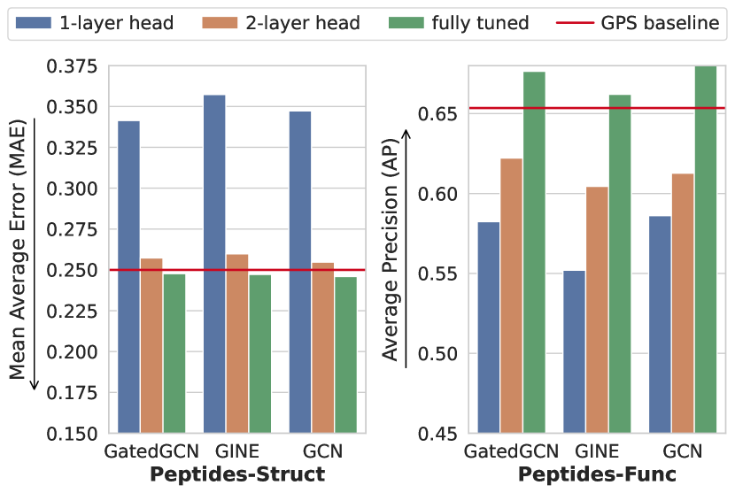
(a) Exchanging the linear prediction head by an MLP accounts for most of the additional performance of all three MPGNNs, especially on Peptides-Struct

Figure 1: On both Peptides datasets, all three MPGNNs surpass GPS. On Peptides-Struct a basic GCN model even achieves SOTA results.

Hyperparameters

In this paper, we argue that the results reported by Dwivedi et al. [1] are not representative for MPGNNs and suffer from suboptimal hyperparameters. We provide new results for the same MPGNN architectures that are obtained after a basic hyperparameter sweep. We tune the main hyperparameters (such as depth, dropout rate, …) in pre-defined ranges while strictly adhering to the official 500k parameter budget. The exact hyperparameter ranges and all final configurations are provided in Section A.1. As a point of reference, we reevalute GPS in an identical manner and also achieve significantly improved results on three datasets with this Graph Transformer. The results reported for GPS may therefore also be subject to suboptimal configurations. Note that we also view the usage of positional or structural encoding (none / LapPE [10] / RWSE [25]) as a hyperparameter that is tuned for each method, including all MPGNNs.

Feature Normalization

The vision datasets PascalVOC-SP and COCO-SP have multi-dimensional node and edge features with values spanning different orders of magnitude for different feature channels. Passing this input to a neural network without channel-wise normalization can cause poorly conditioned activations. While feature normalization is standard practice in deep learning and computer vision in particular, neither Dwivedi et al. [1] nor any subsequent works using LRGB utilize it, except CRaWl [21]. We apply channel-wise linear normalization to all input features and show that all models (baselines and GPS) profit from it in an ablation in Figure 2(a).

Link Prediction Metrics

The evaluation metric on the link-prediction dataset PCQM-Contact [1] is the Mean Reciprocal Rank (MRR) in a filtered setting, as defined by Bordes et al. [26]. For predicted edge scores the MRR measures how a given true edge $(h,t)$ is ranked compared to all possible candidate edges $(h,x)$ of the same head. As there might be multiple true tails $t$ for each head $h$, the filtered MRR removes those other true tails (false negatives) from the list of candidates before computing the metric. This filtering avoids erroneously low MRR values due to the model preferring other true edges and is common in link-prediction tasks. Even though Dwivedi et al. [1] explicitly define the metric to be the filtered MRR, the provided code computes the raw MRR, i.e. keeping other true tails in the list. We report results on PCQM-Contact in a corrected filtered setting. We additionally provide results with an extended filtering procedure where self-loops of the form $(h,h)$ are also removed from the set of candidates, since these are semantically meaningless and never positive. This is impactful as the scoring function used by Dwivedi et al. [1] is based on a symmetric dot-product and therefore exhibits a strong bias towards self-loops.

3 Experiments

	Method	PASCALVOC-SP		COCO-SP
		Test F1 $\uparrow$	rel imp​​​​​​	Test F1 $\uparrow$	​​rel imp​​​
LRGB	GCN	0.1268 ± 0.0060  ⋆		0.0841 ± 0.0010  ⋆
	GINE	0.1265 ± 0.0076  ⋆		0.1339 ± 0.0044  ⋆
	GatedGCN	0.2873 ± 0.0219  ⋆		0.2641 ± 0.0045  ⋆
	Transformer	0.2694 ± 0.0098  ⋆		0.2618 ± 0.0031  ⋆
	SAN	0.3230 ± 0.0039  ⋆		0.2592 ± 0.0158  ⋆
	GPS	0.3748 ± 0.0109  ⋆		0.3412 ± 0.0044  ⋆
Ours	GCN	0.2078 ± 0.0031	+64%	0.1338 ± 0.0007	+59%
	GINE	0.2718 ± 0.0054	+115%	0.2125 ± 0.0009	+59%
	GatedGCN	0.3880 ± 0.0040	+35%	0.2922 ± 0.0018	+11%
	GPS	0.4440 ± 0.0065	+18%	0.3884 ± 0.0055	+13%
Others	CRaWl	0.4588 ± 0.0079		-
	DRew	0.3314 ± 0.0024  ⋆		-
	Exphormer	0.3960 ± 0.0027  ⋆		0.3430 ±0.0008  ⋆

(a) Tuning results on vision datasets PascalVOC-SP and COCO-SP. ^⋆No normalization used.

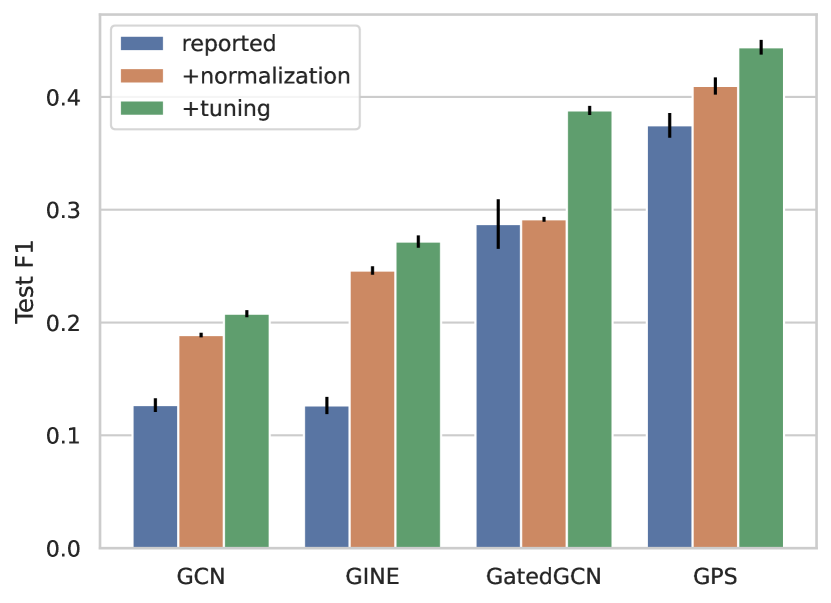
(a) The effects of feature normalization and hyperparameter tuning on PascalVOC-SP.

Figure 2: On PascalVOC-SP and COCO-SP feature normalization and further tuning improves performance across all compared methods.

Peptides-Func and Peptides-Struct

Table 1(a) provides the results obtained on the test splits of the Peptides-Func and Peptides-Struct. For the MPGNN baselines we observe considerable improvements on both datasets as all three MPGNNs outperform GPS after tuning. The average precision on Peptides-Func increased relatively by around 10% to 20%. GCN achieves a score of 68.60%, which is competitive with newer GTs such as GRIT or Graph ViT. The improvement on Peptides-Struct is even more significant with a relative reduction of the MAE of 30%, fully closing the gap to recently proposed GTs. Surprisingly, a simple GCN is all you need to match the best known results on Peptides-Struct. The results for GPS effectively stayed the same as in the original paper [5]. Those values thus seem to be representative for GPS.

We observed that the key hyperparameter underlying the improvements of all three MPGNNs is the depth of the prediction head. To show this Figure 1(a) contains an ablation where we exchanged the linear prediction head configured by Dwivedi et al. [1] with a 2-layer perceptron, keeping all other hyperparameters the same. While the benefit on Peptides-Func is considerable and highly significant, on Peptides-Struct the head depth accounts for almost the complete performance gap between MPGNNs and GTs. GPS’ performance with linear and deeper prediction heads is largely unchanged. For example, our GPS configurations in Table 1(a) use a 2-layer prediction head. Our results indicate that the prediction targets of both datasets appear to depend non-linearly on global graph information. In this case, MPGNNs with linear prediction heads are unable to model the target function. Graph Transformers are not as sensitive to linear prediction heads, since each layer can process global graph information with a deep feed-forward network. However, we would argue that switching to a deep predictive head represents a simpler and computationally cheaper solution to the same issue.

PascalVOC-SP and COCO-SP

Table 2(a) provides the results obtained on the test splits of the superpixel datasets PascalVOC-SP and COCO-SP. We observe significant improvements for all evaluated methods. On PascalVOC-SP the F1 score of GatedGCN increases to 38.80% which exceeds the original performance reported for GPS by Rampášek et al. [5]. GPS also improves significantly to 44.40% F1. This is only one percentage point below the results achieved by CRaWl, which currently is the only reported result with normalized features. The previously large performance gap between GPS and CRaWl is therefore primarily explained by GPS processing raw input signals. On COCO-SP, we observe similar results. Here GPS sets a new state-of-the-art F1 score of 38.84%.

Note that these improvements are achieved entirely through data normalization and hyperparameter tuning. Figure 2(a) provides an ablation on the individual effect of normalization. We train intermediate models with configurations identical to those used by Dwivedi et al. [1] and Rampášek et al. [5], but with feature normalization. For GatedGCN we observe a slight performance increase but a large reduction in the variance across random seeds. For the remaining methods, including GPS, normalization of node and edge features already accounts for at least half of the observed performance gain, emphasizing its importance in practice.

PCQM-Contact

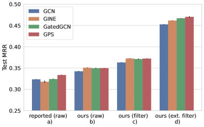
Figure 3: Results on PCQM-Contact. For our own models we provide the MRR scores with varying levels of filtering.

Figure 3 plots the MRR scores obtained on the test split with various evaluation settings as described in the link prediction paragraph of Section 2. First, we provide the results originally reported for LRGB in the literature (a). Recall that these values are obtained in a raw setting with false negatives present. We then provide results obtained after training our own model with new hyperparameters (chosen based on the raw MRR) in b). We still use the raw MRR for evaluation in b) to measure the impact of hyperparameter tuning. Tuning yields an absolute improvement of around 3%. The previously reported slight performance edge of GPS is not observable in this setting after tuning.

In subplot c) we measure the MRR of our models in the filtered setting. Note that these values are based on the exact same predictions as in b), but false negatives are removed. The measured MRR increases by roughly 3% when compared to the raw setting. This shift could erroneously be interpreted as a significant improvement when comparing to literature values obtained in a raw setting. In d) we evaluate our models (still using the same predictions) in an extended filtered setting where we additionally remove self-loops from the candidate pool. Compared to the filtered MRR in c) the MRR metric increases by about 10 percentage points, indicating that self-loops strongly affect the results. Note that in d) GPS again slightly outperforms the MPGNN baselines, in contrast to b) and c). This means that GPS’ predictions seem to suffer overproportionally when self-loops are not filtered. Therefore, the specific choice of how negative samples are filtered on PCQM-Contact can directly affect the ranking of compared methods and must be considered and implemented with care.

4 Conclusion

In our experiments we observed considerable performance gains for all three MPGNN baselines. First, this indicates that extensive baseline tuning is important for properly assessing one’s own method, escpecially on relatively recent datasets. And second, only on the two superpixel datasets graph transformers exhibit clear performance benefits against MPGNNs, indicating that either there are ways to solve the other tasks without long-range interactions or graph transformers are not inherently better at exploiting such long-range dependencies. Evaluating this further appears to be promising direction for future research. In addition, we would invite a discussion on the best-suited link prediction metric on PCQM-Contact.

Appendix A Experiment Details

A.1 Hyperparameters

In the following we describe our methodology for tuning hyperparameters on the LRGB datasets. We did not conduct a dense grid search, since this would be infeasible for all methods and datasets. Instead we perform a “linear” hyperparameter search. We start from a empricially chosen default config and tune each hyperparameter individually within a fixed range. Afterwards, we also evaluate the configuration obtained by combining the best choices of every hyperparameter. From all tried configurations we then select the one with the best validation performance as our final setting. For this hyperparameter sweep, we resorted to a single run per configuration and for the larger datasets slightly reduced the number of epochs. For the final evaluations runs we average results across four different random seeds as specified by the LRGB dataset.

Overall, we tried to incorporate the most important hyperparameters which we selected to be dropout, model depth, prediction head depth, learning rate, and the used positional or structural encoding. For GPS we additionally evaluated the internal MPGNN (but only between GCN and GatedGCN) and whether to use BatchNorm or LayerNorm. Thus, our hyperparamters and ranges were as follows:

• Dropout [0, 0.1, 0.2], default 0.1

• Depth [6,8,10], default 8. The hidden dimension is chosen to stay within a hard limit of 500k parameters

• learning rate [0.001, 0.0005, 0.0001], default $0.001$

• Head depth [1,2,3], default 2

• Encoding [none, LapPE, RWSE] default none

• Internal MPGNN [GCN, GatedGCN], default GatedGCN (only for GPS)

• Normalization [BatchNorm, LayerNorm] default BatchNorm (only for GPS)

On the larger datasets PCQM-Contact and COCO we reduce the hyperparameters budget slightly for efficiency. There, we did not tune the learning rate (it had been $0.001$ in every single other case) and omitted a dropout rate of 0. We note that the tuning procedure used here is relatively simple and not exhaustive. The ranges we searched are rather limited, especially in terms of network depth, and could be expanded in the future. Tables 2, 3, 4, 5 and 6 provide all final model configurations after tuning. Table 7 provides the final performance on all datasets.

We make some additional setup changes based on preliminary experiments. All models are trained with an AdamW optimizer using a cosine annealing learning rate schedule and linear warmup. This differs from Dwivedi et al. [1], who optimized the MPGNN models with a “Reduce on Plateau” schedule and instead matches the learning rate schedule of GPS [5]. We set the weight decay to 0.0 in all five datasets and switch to slightly larger batch sizes to speed up convergence. We also choose GeLU [27] as our default activation function. Furthermore, we change the prediction head for graph-level tasks such that all hidden layers have the same hidden dimension as the GNN itself. These were previously configured to become more narrow with depth, but we could not observe any clear benefit from this design choice. Last, all MPGNN models use proper skip connections which go around the entire GNN layer. The original LRGB results use an implementation of GCN as provided by GraphGym [28]. The skip connections in this implementation do not skip the actual non-linearity at the end of each GCN layer, possibly hindering the flow of gradients. We reimplement GCN with skip connections that go around the non-linearity. Note that these additional tweaks are not used in our ablation studies in Figure 1(a) and Figure 2(a) when training the intermediate models where we only change the head depth and normalization, respectively. There, we use identical model configurations to those used in the literature.

A.2 Feature Normalization

On PascalVOC-SP and COCO-SP we apply channel-wise normalisation to the node and edge features. For each dataset, we compute the channel-wise mean $\mu\in\mathbb{R}^{d}$ and standard deviation $\sigma\in\mathbb{R}^{d}$ on the train split. Here, $d$ is the feature dimension. Each feature vector $x\in\mathbb{R}^{d}$ is then normalized linearly before beigng passed to the model:

$$\tilde{x}_{i}=\frac{x_{i}-\mu_{i}}{\sigma_{i}}$$

Table 2: Hyperparameters on Peptides-Func

	GCN	GINE	GatedGCN	GPS
lr	0.001	0.001	0.001	0.001
dropout	0.1	0.1	0.1	0.1
#layers	6	8	10	6
hidden dim.	235	160	95	76
head depth	3	3	3	2
PE/SE	RWSE	RWSE	RWSE	LapPE
batch size	200	200	200	200
#epochs	250	250	250	250
norm	-	-	-	BatchNorm
MPNN	-	-	-	GatedGCN
#Param.	486k	491k	493k	479k

Table 3: Hyperparameters on Peptides-Struct.

	GCN	GINE	GatedGCN	GPS
lr	0.001	0.001	0.001	0.001
dropout	0.1	0.1	0.1	0.1
#layers	6	10	8	8
hidden dim.	235	145	100	64
head depth	3	3	3	2
PE/SE	LapPE	LapPE	LapPE	LapPE
batch size	200	200	200	200
#epochs	250	250	250	250
norm	-	-	-	BatchNorm
MPNN	-	-	-	GatedGCN
#Param.	488k	492k	445k	452k

Table 4: Hyperparameters on PascalVOC-SP.

	GCN	GINE	GatedGCN	GPS
lr	0.001	0.001	0.001	0.001
dropout	0.0	0.2	0.2	0.1
#layers	10	10	10	8
hidden dim.	200	145	95	68
head depth	3	2	2	2
PE/SE	RWSE	none	none	LapPE
batch size	50	50	50	50
#epochs	200	200	200	200
norm	-	-	-	BatchNorm
MPNN	-	-	-	GatedGCN
#Param.	490k	450k	473k	501k

Table 5: Hyperparameters on COCO-SP.

	GCN	GINE	GatedGCN	GPS
lr	0.001	0.001	0.001	0.001
dropout	0.1	0.1	0.1	0.1
#layers	6	6	8	8
hidden dim.	280	195	105	68
head depth	1	1	1	1
PE/SE	none	none	none	none
batch size	50	50	50	50
#epochs	200	200	200	200
norm	-	-	-	LayerNorm
MPNN	-	-	-	GatedGCN
#Param.	500k	478k	459k	500k

Table 6: Hyperparameters on PCQM-Contact.

	GCN	GINE	GatedGCN	GPS
lr	0.001	0.001	0.001	0.001
dropout	0.1	0.1	0.1	0.0
#layers	8	8	8	6
hidden dim.	215	160	105	76
head depth	1	1	1	1
PE/SE	LapPE	LapPE	LapPE	LapPE
batch size	500	500	500	500
#epochs	150	150	150	150
norm	-	-	-	LayerNorm
MPNN	-	-	-	GatedGCN
#Param.	456k	466k	477k	478k

Table 7: Performance of our models on the Long-Range Graph Benchmark.

Method	PASCALVOC-SP	COCO-SP	PEPTIDES-FUNC	PEPTIDES-STRUCT	PCQM-CONTACT
	Test F1 $\uparrow$	Test F1 $\uparrow$	Test AP $\uparrow$	Test MAE $\downarrow$	Test MRR $\uparrow$
					raw	filter	ext. filter
GCN	0.2078 ± 0.0031	0.1338 ± 0.0007	0.6860 ± 0.0050	0.2460 ± 0.0007	0.3424 ± 0.0007	0.3631 ± 0.0006	0.4526 ± 0.0006
GINE	0.2718 ± 0.0054	0.2125 ± 0.0009	0.6621 ± 0.0067	0.2473 ± 0.0017	0.3509 ± 0.0006	0.3725 ± 0.0006	0.4617 ± 0.0005
GatedGCN	0.3880 ± 0.0040	0.2922 ± 0.0018	0.6765 ± 0.0047	0.2477 ± 0.0009	0.3495 ± 0.0010	0.3714 ± 0.0010	0.4670 ± 0.0004
GPS	0.4440 ± 0.0065	0.3884 ± 0.0055	0.6534 ± 0.0091	0.2509 ± 0.0014	0.3498 ± 0.0005	0.3722 ± 0.0005	0.4703 ± 0.0014

References

- Dwivedi et al. [2022] Vijay Prakash Dwivedi, Ladislav Rampášek, Michael Galkin, Ali Parviz, Guy Wolf, Anh Tuan Luu, and Dominique Beaini. Long range graph benchmark. Advances in Neural Information Processing Systems, 35:22326–22340, 2022.
- Kipf and Welling [2017] Thomas N. Kipf and Max Welling. Semi-supervised classification with graph convolutional networks. In International Conference on Learning Representations (ICLR), 2017.
- Hu et al. [2020a] Weihua Hu, Bowen Liu, Joseph Gomes, Marinka Zitnik, Percy Liang, Vijay Pande, and Jure Leskovec. Strategies for pre-training graph neural networks. In International Conference on Learning Representations, 2020a. URL https://openreview.net/forum?id=HJlWWJSFDH.
- Bresson and Laurent [2017] Xavier Bresson and Thomas Laurent. Residual gated graph convnets. arXiv preprint arXiv:1711.07553, 2017.
- Rampášek et al. [2022] Ladislav Rampášek, Michael Galkin, Vijay Prakash Dwivedi, Anh Tuan Luu, Guy Wolf, and Dominique Beaini. Recipe for a general, powerful, scalable graph transformer. Advances in Neural Information Processing Systems, 35:14501–14515, 2022.
- Hamilton et al. [2017] William L. Hamilton, Zhitao Ying, and Jure Leskovec. Inductive representation learning on large graphs. pages 1024–1034, 2017.
- Xu et al. [2018] Keyulu Xu, Weihua Hu, Jure Leskovec, and Stefanie Jegelka. How powerful are graph neural networks? arXiv preprint arXiv:1810.00826, 2018.
- Chen et al. [2020] Ming Chen, Zhewei Wei, Zengfeng Huang, Bolin Ding, and Yaliang Li. Simple and deep graph convolutional networks. In International conference on machine learning, pages 1725–1735. PMLR, 2020.
- Corso et al. [2020] Gabriele Corso, Luca Cavalleri, Dominique Beaini, Pietro Liò, and Petar Velickovic. Principal neighbourhood aggregation for graph nets. In Hugo Larochelle, Marc’Aurelio Ranzato, Raia Hadsell, Maria-Florina Balcan, and Hsuan-Tien Lin, editors, Advances in Neural Information Processing Systems 33: Annual Conference on Neural Information Processing Systems 2020, NeurIPS 2020, December 6-12, 2020, virtual, 2020. URL https://proceedings.neurips.cc/paper/2020/hash/99cad265a1768cc2dd013f0e740300ae-Abstract.html.
- Dwivedi and Bresson [2020] Vijay Prakash Dwivedi and Xavier Bresson. A generalization of transformer networks to graphs. arXiv preprint arXiv:2012.09699, 2020.
- Ying et al. [2021] Chengxuan Ying, Tianle Cai, Shengjie Luo, Shuxin Zheng, Guolin Ke, Di He, Yanming Shen, and Tie-Yan Liu. Do transformers really perform badly for graph representation? Advances in Neural Information Processing Systems, 34:28877–28888, 2021.
- Kreuzer et al. [2021] Devin Kreuzer, Dominique Beaini, Will Hamilton, Vincent Létourneau, and Prudencio Tossou. Rethinking graph transformers with spectral attention. Advances in Neural Information Processing Systems, 34:21618–21629, 2021.
- Shi et al. [2020] Yunsheng Shi, Zhengjie Huang, Shikun Feng, Hui Zhong, Wenjin Wang, and Yu Sun. Masked label prediction: Unified message passing model for semi-supervised classification. arXiv preprint arXiv:2009.03509, 2020.
- Park et al. [2022] Wonpyo Park, Woonggi Chang, Donggeon Lee, Juntae Kim, and Seung-won Hwang. Grpe: Relative positional encoding for graph transformer. arXiv preprint arXiv:2201.12787, 2022.
- Weis et al. [2021] Marissa A Weis, Laura Pede, Timo Lüddecke, and Alexander S Ecker. Self-supervised representation learning of neuronal morphologies. arXiv preprint arXiv:2112.12482, 2021.
- Shirzad et al. [2023] Hamed Shirzad, Ameya Velingker, Balaji Venkatachalam, Danica J Sutherland, and Ali Kemal Sinop. Exphormer: Sparse transformers for graphs. In International Conference on Machine Learning, 2023.
- Kim et al. [2022] Jinwoo Kim, Dat Nguyen, Seonwoo Min, Sungjun Cho, Moontae Lee, Honglak Lee, and Seunghoon Hong. Pure transformers are powerful graph learners. Advances in Neural Information Processing Systems, 35:14582–14595, 2022.
- Ma et al. [2023] Liheng Ma, Chen Lin, Derek Lim, Adriana Romero-Soriano, K. Dokania, Mark Coates, Philip H.S. Torr, and Ser-Nam Lim. Graph Inductive Biases in Transformers without Message Passing. In Proc. Int. Conf. Mach. Learn., 2023.
- He et al. [2023] Xiaoxin He, Bryan Hooi, Thomas Laurent, Adam Perold, Yann Lecun, and Xavier Bresson. A generalization of ViT/MLP-mixer to graphs. In Andreas Krause, Emma Brunskill, Kyunghyun Cho, Barbara Engelhardt, Sivan Sabato, and Jonathan Scarlett, editors, Proceedings of the 40th International Conference on Machine Learning, volume 202 of Proceedings of Machine Learning Research, pages 12724–12745. PMLR, 23–29 Jul 2023. URL https://proceedings.mlr.press/v202/he23a.html.
- Min et al. [2022] Erxue Min, Runfa Chen, Yatao Bian, Tingyang Xu, Kangfei Zhao, Wenbing Huang, Peilin Zhao, Junzhou Huang, Sophia Ananiadou, and Yu Rong. Transformer for graphs: An overview from architecture perspective. arXiv preprint arXiv:2202.08455, 2022.
- Tönshoff et al. [2021] Jan Tönshoff, Martin Ritzert, Hinrikus Wolf, and Martin Grohe. Graph learning with 1d convolutions on random walks. CoRR, abs/2102.08786, 2021. URL https://arxiv.org/abs/2102.08786.
- Gutteridge et al. [2023] Benjamin Gutteridge, Xiaowen Dong, Michael M. Bronstein, and Francesco Di Giovanni. DRew: Dynamically rewired message passing with delay. In Andreas Krause, Emma Brunskill, Kyunghyun Cho, Barbara Engelhardt, Sivan Sabato, and Jonathan Scarlett, editors, Proceedings of the 40th International Conference on Machine Learning, volume 202 of Proceedings of Machine Learning Research, pages 12252–12267. PMLR, 23–29 Jul 2023. URL https://proceedings.mlr.press/v202/gutteridge23a.html.
- Dwivedi et al. [2020] Vijay Prakash Dwivedi, Chaitanya K Joshi, Thomas Laurent, Yoshua Bengio, and Xavier Bresson. Benchmarking graph neural networks. arXiv preprint arXiv:2003.00982, 2020.
- Hu et al. [2020b] Weihua Hu, Matthias Fey, Marinka Zitnik, Yuxiao Dong, Hongyu Ren, Bowen Liu, Michele Catasta, and Jure Leskovec. Open graph benchmark: Datasets for machine learning on graphs. In Hugo Larochelle, Marc’Aurelio Ranzato, Raia Hadsell, Maria-Florina Balcan, and Hsuan-Tien Lin, editors, Advances in Neural Information Processing Systems 33: Annual Conference on Neural Information Processing Systems 2020, NeurIPS 2020, December 6-12, 2020, virtual, 2020b. URL https://proceedings.neurips.cc/paper/2020/hash/fb60d411a5c5b72b2e7d3527cfc84fd0-Abstract.html.
- Dwivedi et al. [2021] Vijay Prakash Dwivedi, Anh Tuan Luu, Thomas Laurent, Yoshua Bengio, and Xavier Bresson. Graph neural networks with learnable structural and positional representations. In International Conference on Learning Representations, 2021.
- Bordes et al. [2013] Antoine Bordes, Nicolas Usunier, Alberto Garcia-Duran, Jason Weston, and Oksana Yakhnenko. Translating embeddings for modeling multi-relational data. In C.J. Burges, L. Bottou, M. Welling, Z. Ghahramani, and K.Q. Weinberger, editors, Advances in Neural Information Processing Systems, volume 26. Curran Associates, Inc., 2013. URL https://proceedings.neurips.cc/paper_files/paper/2013/file/1cecc7a77928ca8133fa24680a88d2f9-Paper.pdf.
- Hendrycks and Gimpel [2016] Dan Hendrycks and Kevin Gimpel. Gaussian error linear units (gelus). arXiv preprint arXiv:1606.08415, 2016.
- You et al. [2020] Jiaxuan You, Zhitao Ying, and Jure Leskovec. Design space for graph neural networks. Advances in Neural Information Processing Systems, 33:17009–17021, 2020.