Coexistence of nematic superconductivity and spin density wave in magic-angle twisted bilayer graphene

Abstract

We argue that doped twisted bilayer graphene with magical twist angle can become superconducting. In our theoretical scenario the superconductivity coexists with the spin-density-wave-like ordering. Numerical mean field analysis demonstrates that the spin-density wave order, which is much stronger than the superconductivity, leaves parts of the Fermi surface ungapped. This Fermi surface serves as a host for the superconductivity. Since the magnetic texture at finite doping breaks the point group of the twisted bilayer graphene, the stabilized superconducting order parameter is nematic. We also explore the possibility of purely Coulomb-based mechanism of the superconductivity in the studied system. The screened Coulomb interaction is calculated within the random phase approximation. It is shown that near the half-filling the renormalized Coulomb repulsion indeed induces the superconducting state, with the order parameter possessing two nodes on the Fermi surface. We estimate the superconducting transition temperature, which turns out to be very low. The implications of our proposal are discussed.

I Introduction

The discovery of Mott insulating states Cao et al. (2018a); Lu et al. (2019) and superconductivity Cao et al. (2018b); Lu et al. (2019) in magic angle twisted bilayer graphene (MAtBLG) has attracted great attention to this material. In twisted bilayer graphene (tBLG) one graphene layer is rotated with respect to another one by a twist angle $\theta$. The twisting produces moiré pattern and superstructure in the system. Low-energy electronic structure of tBLG is substantially modified in comparison to single-layer, AA-stacked, and AB-stacked bilayer graphene Rozhkov et al. (2016). For small $\theta\sim 1^{\circ}$, the low-energy single-electron spectrum consists of eight (if spin degree of freedom is accounted for) flat bands separated from lower and higher dispersive bands by energy gaps Rozhkov et al. (2016); Lopes dos Santos et al. (2012); San-Jose et al. (2012). The width of the low-energy bands (which is about several meV) has a minimum at $\theta=\theta_{c}$, where $\theta_{c}$ is the so-called magic angle $\theta_{c}\sim 1^{\circ}$.

The existence of the flat bands makes MAtBLG very susceptible to interactions. The interactions lead to the appearance of Mott insulating states when carrier doping per superlattice cell $n$ is integer. Authors of Ref. Cao et al., 2018a observed the insulating states in transport measurements near the neutrality point (zero doping) and at doping corresponding to $n=\pm 2$ extra charges per supercell. In similar experiments in Ref. Lu et al., 2019 the authors observed Mott states at doping corresponding to $n=0$, $n=\pm 1$, $n=\pm 2$, and $n=\pm 3$. The nature of the insulating ground states is under discussion Padhi et al. (2018); Ochi et al. (2018); Liu et al. (2018); Huang et al. (2019); Sboychakov et al. (2019); Sboychakov et al. (2020a); Sboychakov et al. (2022); Sboychakov et al. (2020b); Cea and Guinea (2020); Hofmann et al. (2022); Song and Bernevig (2022); Wagner et al. (2022); Seo et al. (2019). Several types of ordering, such as spin-density wave (SDW) states Liu et al. (2018); Huang et al. (2019); Sboychakov et al. (2019); Sboychakov et al. (2020a); Sboychakov et al. (2022), ferromagnetic state Seo et al. (2019), and other symmetry-broken phases Cea and Guinea (2020); Hofmann et al. (2022); Wagner et al. (2022); Song and Bernevig (2022) have been proposed to be the ground state of the system.

Besides Mott insulating states, the authors of Ref. Cao et al., 2018b observed on the doping-temperature ($n,T$) plane two superconductivity domes located slightly below and slightly above half-filling, $n=-2$. In other experimentsLu et al. (2019), the superconductivity domes have been observed close to $n=-2$, $n=0$, and $n=\pm 1$.

Theory of the superconductivity in the MAtBLG has been developed in many papers, see, e.g., Refs. Wu et al., 2018; Lian et al., 2019; Guo et al., 2018; Liu et al., 2018; González and Stauber, 2019; Huang et al., 2019; Roy and Juričić, 2019; Löthman et al., 2022; Cao et al., 2022; Qin et al., 2023. Different mechanisms, including phonon Wu et al. (2018); Lian et al. (2019); Cao et al. (2022) and electronic Guo et al. (2018); Liu et al. (2018); González and Stauber (2019); Huang et al. (2019); Roy and Juričić (2019), are under discussion. The symmetry of the superconducting order parameter is debated as well. All cited works suggest that the superconductivity does not coexist with any non-superconducting order parameter.

In our previous papers Sboychakov et al. (2019); Sboychakov et al. (2020a, b); Sboychakov et al. (2022) we studied the non-superconducting order in MAtBLG assuming that the SDW is the ground state of the system. We showed that the SDW is stable in the doping range $-4<n<4$. This allowed us to explain the behavior of the conductivity versus doping (of course, that theory is applicable only outside of the regions where superconductivity was observed). We showed also that at finite doping the point symmetry of the SDW state is reduced, and electronic nematicity emerges Sboychakov et al. (2020a). The latter is indeed confirmed by experiment Choi et al. (2019); Kerelsky et al. (2019).

In the present paper we focus on the superconductivity. We consider the doping range close to half-filling, $n=-2$. We assume here that the superconductivity coexists, but does not compete, with the SDW phase. This expectation is based on the observation that the SDW order, with its characteristic energy of several tens of meV, is much stronger than the superconductivity, whose transition temperature is as low as $T_{c}=1.7$ K. Under such circumstances, theoretical justification for the coexistence relies on the presence of a Fermi surface that remains in MAtBLG even when SDW order is established.

Additionally, we investigate a non-phonon mechanism of superconductivity for MAtBLG. Our proposal relies on the renormalized Coulomb potential, which we calculate using the random phase approximation (RPA). It will be demonstrated that the screened Coulomb interaction can indeed stabilize the superconductivity coexisting with the SDW. The superconducting order parameter has two nodes on the Fermi surface, similar to a $p$-wave order. However, as the SDW spin texture breaks several symmetries, the common order-parameter classification into $s$-wave, $p$-wave, etc., does not apply. The estimated critical temperature turns out to be significantly smaller than the experimentally observed values. This discrepancy is discussed from the theory standpoint. Possible reasons behind it are analyzed.

The paper is organized as follows. The geometry of the system under study is briefly described in Sec. II. In Section III we formulate our model and describe the structure of the SDW order parameter. Section IV is devoted to the static polarization operator and the renormalized Coulomb potential. In Section V we derive the self-consistency equation for the superconducting order parameter coexisting with the SDW order. We describe the property of the superconducting order and obtain an estimate for $T_{c}$. Discussion and conclusions are presented in Section VI.

II Geometry of twisted bilayer graphene

In this Section we recap several basic facts about the geometry of the tBLG that are important for further consideration (for more details, see, e.g., reviews Refs. Mele, 2012; Rozhkov et al., 2016). Each graphene layer in tBLG forms a hexagonal honeycomb lattice that can be split into two triangular sublattices, ${\cal A}$ and ${\cal B}$. The coordinates of atoms in layer 1 on sublattices ${\cal A}$ and ${\cal B}$ are

$$\mathbf{r}_{\mathbf{n}}^{1{\cal A}}=\mathbf{r}_{\mathbf{n}}^{1}\equiv n\mathbf{a}_{1}+m\mathbf{a}_{2}\,,\;\;\mathbf{r}_{\mathbf{n}}^{1{\cal B}}=\mathbf{r}_{\mathbf{n}}^{1}+\bm{\delta}\,,$$ (1)

where $\mathbf{n}=(n,\,m)$ is an integer-valued vector, $\mathbf{a}_{1,2}=a(\sqrt{3},\mp 1)/2$ are the primitive vectors, $\bm{\delta}=(\mathbf{a}_{1}+\mathbf{a}_{2})/3=a(1/\sqrt{3},0)$ is a vector connecting two atoms in the same unit cell, and $a=2.46$ Å is the lattice constant of graphene. Atoms in layer 2 are located at

$$\mathbf{r}_{\mathbf{n}}^{2{\cal B}}=\mathbf{r}_{\mathbf{n}}^{2}\equiv d\mathbf{e}_{z}+n\mathbf{a}_{1}^{\prime}+m\mathbf{a}_{2}^{\prime}\,,\quad\mathbf{r}_{\mathbf{n}}^{2{\cal A}}=\mathbf{r}_{\mathbf{n}}^{2}-\bm{\delta}^{\prime}\,,$$ (2)

where $\mathbf{a}_{1,2}^{\prime}$ and $\bm{\delta}^{\prime}$ are the vectors $\mathbf{a}_{1,2}$ and $\bm{\delta}$, rotated by the twist angle $\theta$. The unit vector along the $z$-axis is $\mathbf{e}_{z}$, the interlayer distance is $d=3.35$ Å. The limiting case $\theta=0$ corresponds to the AB stacking.

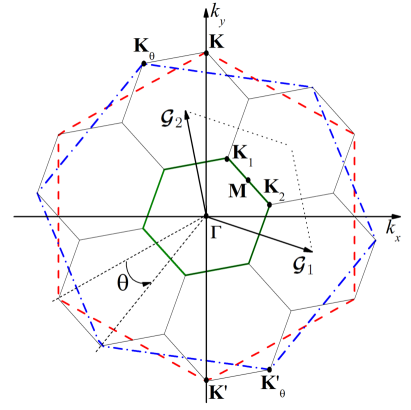
Figure 1: Reciprocal space geometry of tBLG for $\theta\approx 21.79^{\circ}$ ($m_{0}=1$, $r=1$). The figure presents Brillouin zones of layers 1 and 2 (large red and blue hexagons), as well as the Brillouin zone of the superlattice (small thick green hexagon). Reciprocal vectors of the superlattice ($\bm{{\cal G}}_{1}$ and $\bm{{\cal G}}_{2}$), Dirac points of layer 1 ($\mathbf{K}$ and $\mathbf{K}^{\prime}$) and layer 2 ($\mathbf{K}_{\theta}$ and $\mathbf{K}^{\prime}_{\theta}$), as well as high symmetry points of the reduced Brillouin zone ($\bm{\Gamma}$, $\mathbf{M}$, $\mathbf{K}_{1,2}$) are also shown.

Twisting produces moiré patterns Rozhkov et al. (2016), which can be seen as alternating dark and bright regions in STM images. Measuring the moiré period $L$, one can extract the twist angle using the formula $L=a/[2\sin(\theta/2)]$. Moiré patterns exist for arbitrary twist angles. If the twist angle satisfies the relationship

$$\cos\theta=\frac{3m_{0}^{2}+3m_{0}r+r^{2}/2}{3m_{0}^{2}+3m_{0}r+r^{2}}\,,$$ (3)

where $m_{0}$ and $r$ are co-prime positive integers, it is called commensurate. For commensurate $\theta$’s a superstructure emerges, and the sample splits into a periodic lattice of finite supercells. The majority of theoretical papers assume the twist angle to be the commensurate one, since only in this case one can work with Bloch waves and introduce the quasimomentum. For the commensurate structure described by $m_{0}$ and $r$, the superlattice vectors are

$$\mathbf{R}_{1}=m_{0}\mathbf{a}_{1}+(m_{0}+r)\mathbf{a}_{2},\,\mathbf{R}_{2}=-(m_{0}+r)\mathbf{a}_{1}+(m_{0}+2r)\mathbf{a}_{2},$$ (4)

if $r\neq 3n$ ($n$ is an integer), or

$$\mathbf{R}_{1}=(m_{0}+n)\mathbf{a}_{1}+n\mathbf{a}_{2},\,\mathbf{R}_{2}=-n\mathbf{a}_{1}+(m_{0}+2n)\mathbf{a}_{2},$$ (5)

if $r=3n$. The number of graphene unit cells inside a supercell is $N_{\rm sc}=(3m_{0}^{2}+3m_{0}r+r^{2})/g$ per layer. The parameter $g$ in the latter expression is equal to unity when $r\neq 3n$. Otherwise, it is $g=3$.

The superlattice cell of the structure with $m_{0}$ and $r$ contains $r^{2}$ moiré cells if $r\neq 3n$, or $r^{2}/3$ moiré cells otherwise. When $r=1$, the superlattice cell coincides with the moiré cell. In the present paper we consider only such structures. When $\theta$ is small enough, the superlattice cell can be approximately described as consisting of regions with almost AA, AB, and BA stackings Lopes dos Santos et al. (2012); Rozhkov et al. (2016).

The reciprocal lattice primitive vectors for layer 1 (layer 2) are denoted by $\mathbf{b}_{1,2}$ ($\mathbf{b}_{1,2}^{\prime}$). For layer 1 one has $\mathbf{b}_{1,2}=(2\pi/\sqrt{3},\mp 2\pi)/a$, while $\mathbf{b}_{1,2}^{\prime}$ are connected to $\mathbf{b}_{1,2}$ by a rotation of an angle $\theta$. Using the notation $\bm{{\cal G}}_{1,2}$ for the primitive reciprocal vectors of the superlattice, the following identities in the reciprocal space are valid:

$$\mathbf{b}_{1}^{\prime}=\mathbf{b}_{1}+r(\bm{{\cal G}}_{1}+\bm{{\cal G}}_{2})\,,\;\mathbf{b}_{2}^{\prime}=\mathbf{b}_{2}-r\bm{{\cal G}}_{1}\,,$$ (6)

if $r\neq 3n$, or

$$\mathbf{b}_{1}^{\prime}=\mathbf{b}_{1}+n(\bm{{\cal G}}_{1}+2\bm{{\cal G}}_{2})\,,\;\mathbf{b}_{2}^{\prime}=\mathbf{b}_{2}-n(2\bm{{\cal G}}_{1}+\bm{{\cal G}}_{2})\,,$$ (7)

if $r=3n$.

Each graphene layer in tBLG has a hexagonal Brillouin zone. The Brillouin zone of the layer 2 is rotated in momentum space with respect to the Brillouin zone of layer 1 by the twist angle $\theta$. The Brillouin zone of the superlattice (reduced Brillouin zone, RBZ) is also hexagonal but smaller in size. It can be obtained by $N_{\rm sc}$-times folding of the Brillouin zone of the layer 1 or 2. Two non-equivalent Dirac points of the layer 1 can be chosen as $\mathbf{K}=(0,4\pi/(3a)),\mathbf{K}^{\prime}=-\mathbf{K}$. The Dirac points of the layer 2 are $\mathbf{K}_{\theta}=4\pi(-\sin\theta,\cos\theta)/(3a)$, $\mathbf{K}^{\prime}_{\theta}=-\mathbf{K}_{\theta}$. Band folding translates these four Dirac points to the two Dirac points of the superlattice, $\mathbf{K}_{1,2}$. Thus, one can say that the Dirac points of the superlattice are doubly degenerate. Points $\mathbf{K}_{1}$ and $\mathbf{K}_{2}$ can be expressed via vectors $\bm{{\cal G}}_{1,2}$ as

$$\mathbf{K}_{1}=\frac{1}{3}(\bm{{\cal G}}_{1}+2\bm{{\cal G}}_{2})\,,\quad\mathbf{K}_{2}=\frac{1}{3}(2\bm{{\cal G}}_{1}+\bm{{\cal G}}_{2})\,.$$ (8)

A typical picture illustrating these three Brillouin zones, the vectors $\bm{{\cal G}}_{1,2}$, as well as main symmetrical points is shown in Fig. 1.

III Model Hamiltonian

We start with the following Hamiltonian of the tBLG:

$$H = \!\!\!\sum_{{\mathbf{nm}ij\atop ss^{\prime}\sigma}}\!t(\mathbf{r}_{\mathbf{n}}^{is};\mathbf{r}_{\mathbf{m}}^{js^{\prime}})d^{{\dagger}}_{\mathbf{n}is\sigma}d^{\phantom{{\dagger}}}_{\mathbf{m}js^{\prime}\sigma}+U\!\sum_{{\mathbf{n}is}}\!n_{\mathbf{n}is\uparrow}n_{\mathbf{n}is\downarrow}+$$ (9)

$$\frac{1}{2}\!\mathop{{\sum}^{\prime}}_{{\mathbf{nm}ij\atop ss^{\prime}\sigma\sigma^{\prime}}}\!V(\mathbf{r}_{\mathbf{n}}^{is}-\mathbf{r}_{\mathbf{m}}^{js^{\prime}})n_{\mathbf{n}is\sigma}n_{\mathbf{m}js^{\prime}\sigma^{\prime}}\,.$$

In this expression $d^{{\dagger}}_{\mathbf{n}is\sigma}$ ($d^{\phantom{{\dagger}}}_{\mathbf{n}is\sigma}$) are the creation (annihilation) operators of the electron with spin $\sigma$ ($=\uparrow,\downarrow$) at the unit cell $\mathbf{n}$ in the layer $i$ ($=1,2$) in the sublattice $s$ ($={\cal A,B}$), while $n_{\mathbf{n}is\sigma}=d^{{\dagger}}_{\mathbf{n}is\sigma}d^{\phantom{{\dagger}}}_{\mathbf{n}is\sigma}$. The first term in Eq. (9) is the single-particle tight-binding Hamiltonian with $t(\mathbf{r}_{\mathbf{n}}^{is};\mathbf{r}_{\mathbf{m}}^{js^{\prime}})$ being the amplitude of the electron hopping from site in the position $\mathbf{r}_{\mathbf{m}}^{js^{\prime}}$ to the site in the position $\mathbf{r}_{\mathbf{n}}^{is}$. The second term in Eq. (9) describes the on-site (Hubbard) interaction of electrons with opposite spins, while the last term corresponds to the intersite Coulomb interaction [the prime near the last sum in Eq. (9) means that elements with $\mathbf{r}_{\mathbf{n}}^{is}=\mathbf{r}_{\mathbf{m}}^{js^{\prime}}$ should be excluded].

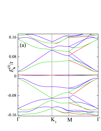
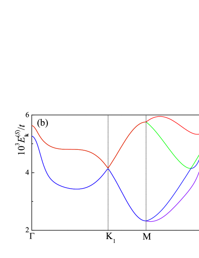
Figure 2: (a) Energy spectrum of MAtBLG at vanishing interactions. The flat bands appears as a bundle of almost non-dispersive horizontal lines at $E_{\bf k}^{(S)}\approx 4\times 10^{-3}t$. The gaps separating the flat bands from the dispersive bands are clearly visible. The data in panel (b) show that the flat bands do have finite dispersion as well. Their width $W$ can be approximately estimated as $W\approx 9.4$ meV

III.1 Single-particle spectrum of MAtBLG

Let us consider first the single-particle properties of the MAtBLG. If we neglect interactions, the electronic spectrum of the system is obtained by diagonalization of the first term of the Hamiltonian (9). The result depends on the parametrization of the hopping amplitudes $t(\mathbf{r}_{\mathbf{n}}^{is};\mathbf{r}_{\mathbf{m}}^{js^{\prime}})$. In this paper we keep only nearest-neighbor terms for the intralayer hopping. The corresponding amplitude is $t=-2.57$ eV.

As for the interlayer hopping amplitudes, we explored several parametrization schemes, all of which deliver qualitatively similar results. The results presented below correspond to the parametrization II.B of Ref. Sboychakov et al., 2020a. This parametrization, initially proposed in Ref. Tang et al., 1996, takes into account the environment dependence of the hopping. That is, the electron hopping amplitude connecting two atoms at positions $\mathbf{r}$ and $\mathbf{r}^{\prime}$ depends not only on the difference $\mathbf{r}-\mathbf{r}^{\prime}$, but also on positions of other atoms in the lattice. Extra flexibility of the formalism becomes useful when the tunneling between $\mathbf{r}$ and $\mathbf{r}^{\prime}$ is depleted by nearby atoms, which act as obstacles to a tunneling electron. For the tBLG, the parametrization II.B was used in Refs. Shallcross et al., 2010; Sboychakov et al., 2015; Rozhkov et al., 2017, among other papers. This parametrization can correctly reproduce the Slonczewski-Weiss-McClure parametrization scheme in the limiting case of the AB bilayer graphene ($\theta=0$).

Once a specific parametrization is chosen, the single-electron Hamiltonian may be diagonalized and its energy spectrum may be found. For parametrization chosen, the magic angle superstructure is $(m_{0},\,r)=(17,\,1)$, which corresponds to the magic angle $\theta_{c}=1.89^{\circ}$.

To execute the Hamiltonian diagonalization, one must introduce the quasi-momentum representation. To this end, we define new electronic operators $d^{\phantom{{\dagger}}}_{\mathbf{pG}is\sigma}$ by the following relation

$$d^{\phantom{{\dagger}}}_{\mathbf{pG}is\sigma}=\frac{1}{\sqrt{{\cal{N}}}}\sum_{\mathbf{n}}\exp{[-i(\mathbf{p}+\mathbf{G})\mathbf{r}_{\mathbf{n}}^{i}]}d_{\mathbf{n}is\sigma}\,,$$ (10)

where ${\cal N}$ is the number of graphene unit cells in the sample in one layer, the momentum $\mathbf{p}$ lies in the first Brillouin zone of the superlattice, while $\mathbf{G}=n\bm{{\cal G}}_{1}+m\bm{{\cal G}}_{2}$ is the reciprocal vector of the superlattice confined to the first Brillouin zone of the $i$th layer. The number of $\mathbf{G}$’s satisfying the latter requirement is equal to $N_{\rm sc}$ for each graphene layer.

In the quasi-momentum representation, for a specific quasi-momentum ${\bf p}$, the single-electron Hamiltonian is a bilinear of the fermionic operators, characterized by a $4N_{\rm sc}\times 4N_{\rm sc}$ matrix (one such matrix per spin projection). Diagonalizing this matrix numerically, one finds the single-electron spectrum of tBLG. The low-energy part of the spectrum is shown in Fig. 2. In this figure we see four flat bands $E_{0\mathbf{k}}^{({\cal S})}$ separated from lower and higher dispersive bands by the energy gaps of the order of $30$ meV. The width of the flat bands $W$ as a function of the twist angle $\theta$ has a minimum $W=9.4$ meV at the magic angle.

Unlike undoped graphene and undoped AB bilayer, which both have Fermi points, tBLG at low $\theta$ is a metal Sboychakov et al. (2015) even at no doping. The four flat bands cross the Fermi level forming multi-component Fermi surface, see Fig. 8 in Ref. Sboychakov et al., 2015. The shape of the Fermi surface components depend on the specific model of the interlayer hopping and on the doping level $n$.

III.2 SDW order parameters

The system having flat bands intersecting the Fermi level is very susceptible to interactions. Interactions spontaneously break symmetries of the single-particle Hamiltonian generating an order parameter. Neglecting first a possibility of the superconducting state, we assume that this order parameter is the SDW. This choice is not arbitrary. It was shown in many papers (see, e.g., Refs. Lopes dos Santos et al., 2012; San-Jose et al., 2012; Sboychakov et al., 2015), that at small twist angles, electrons on the Fermi level occupy mainly the regions with almost perfect AA stacking within a supercell. At the same time, it was demonstrated theoretically Rakhmanov et al. (2012); Sboychakov et al. (2013a, b); Akzyanov et al. (2014) that the ground state of AA stacked bilayer graphene is antiferromagnetic. For this reason, we believe that the ground state of MAtBLG possesses an SDW-like order parameter.

The SDW order parameter is a multicomponent one. First, it contains on-site terms of the form

$$\Delta_{\mathbf{n}is}=U\langle d^{{\dagger}}_{\mathbf{n}is\uparrow}d^{\phantom{{\dagger}}}_{\mathbf{n}is\downarrow}\rangle\,,$$ (11)

with the on-site interaction $U$ serving as a proportionality coefficient. For our calculations we assign $U=2t$. This value of $U$ is somewhat smaller than the critical $U_{c}=2.23t$ above which single-layer graphene spontaneously enters a mean-field antiferromagnetic state Sorella and Tosatti (1992). Thus, our Hubbard interaction is rather strong, but not strong enough to open a gap in single-layer graphene.

Next, we include an intralayer nearest-neighbor SDW order parameter, which is defined on links connecting nearest neighbor atoms in the same layer. In a graphene layer, each atom in one sublattice has three nearest neighbors belonging to the opposite sublattice: an atom on sublattice ${\cal B}$ (sublattice ${\cal A}$) has three nearest neighbors on sublattice ${\cal A}$ (sublattice ${\cal B}$). For this reason we consider three types of intralayer nearest-neighbor order parameters, $A^{(\ell)}_{\mathbf{n}i\sigma}$ ($\ell=1,\,2,\,3$), corresponding to three different links connecting the nearest-neighbor sites. These order parameters are defined as follows

$$A^{(\ell)}_{\mathbf{n}i\sigma}=V_{\rm nn}\langle d^{{\dagger}}_{\mathbf{n}+\mathbf{n}_{\ell}i{\cal A}\sigma}d^{\phantom{{\dagger}}}_{\mathbf{n}i{\cal B}\bar{\sigma}}\rangle\,,$$ (12)

where $\mathbf{n}_{1}=(0,\,0)$, $\mathbf{n}_{2}=(1,\,0)$, $\mathbf{n}_{3}=(0,\,1)$, $\bar{\sigma}=-\sigma$, and $V_{\rm nn}=V(|\bm{\delta}|)$ is the in-plane nearest-neighbor Coulomb repulsion. We take $V_{\text{nn}}/U=0.59$, in agreement with Ref. Wehling et al., 2011.

Finally, we introduce the interlayer SDW order parameter

$$B^{rs}_{\mathbf{m};\mathbf{n}\sigma}=V(\mathbf{r}^{1r}_{\mathbf{m}}-\mathbf{r}^{2s}_{\mathbf{n}})\langle d^{{\dagger}}_{\mathbf{m}1r\sigma}d^{\phantom{{\dagger}}}_{\mathbf{n}2s\bar{\sigma}}\rangle\,.$$ (13)

For calculations it is assumed that $B^{rs}_{\mathbf{m};\mathbf{n}\sigma}$ is non-zero only when sites $\mathbf{r}_{\mathbf{m}}^{1s}$ and $\mathbf{r}_{\mathbf{n}}^{2r}$ are sufficiently close. Namely, if the hopping amplitude connecting $\mathbf{r}_{\mathbf{m}}^{1s}$ and $\mathbf{r}_{\mathbf{n}}^{2r}$ vanishes in our computation scheme, then, the parameter $B^{rs}_{\mathbf{m};\mathbf{n}\sigma}$ is also zero. Naturally, the number of non-zero $B^{rs}_{\mathbf{m};\mathbf{n}\sigma}$ depends on the type of the hopping amplitude parametrization. For parametrization chosen we have up to three non-zero $B^{rs}_{\mathbf{m};\mathbf{n}\sigma}$ for a given $\mathbf{n}$, $r$, $s$, and $\sigma$. Assuming that the screening is small at short distances, we chose the function $V(\mathbf{r})$ in Eq. (13) as $V(\mathbf{r})\propto 1/|\mathbf{r}|$ with $V(d)=V_{\text{nn}}|\bm{\delta}|/d=0.25U$. All three types of SDW order parameters are restricted to obey the superlattice periodicity.

Using these order parameters, the full MAtBLG Hamiltonian can be approximated by a mean field Hamiltonian, the latter being quadratic in fermionic operators. The mean field Hamiltonian is uniquely specified by a $8N_{\rm sc}\times 8N_{\rm sc}$ matrix. This matrix diagonalization allows one to determine the eigenfunctions $\Phi_{\mathbf{pG}is\sigma}^{(S)}$ and eigenvalues $E^{(S)}_{\bf p}$ of the mean field Hamiltonian, as well as the mean field ground state energy for a fixed $n$. The Bogolyubov transformation

$$d^{\phantom{{\dagger}}}_{\mathbf{pG}is\sigma}=\sum_{S}\Phi_{\mathbf{pG}is\sigma}^{(S)}\psi_{\mathbf{p}S}\,,$$ (14)

introduces new Fermi operators $\psi_{\mathbf{p}S}$ that diagonalize the mean field Hamiltonian.

Minimizing the mean field ground state energy, one derives the self-consistency equations for $\Delta_{\mathbf{n}is}$, $A^{(\ell)}_{\mathbf{n}i\sigma}$, and $B^{rs}_{\mathbf{m};\mathbf{n}\sigma}$. These equations must be solved numerically for different values of doping $n$ confined to the interval $-4<n<4$. The details of the numerical procedure can be found in Ref. Sboychakov et al., 2020a.

III.3 Symmetry properties of the order parameters

The results of the order parameters calculations for different doping levels are presented in Ref. Sboychakov et al., 2020a, where spatial profiles of $\Delta_{\mathbf{n}is}$ and $A^{(\ell)}_{\mathbf{n}i\sigma}$ are plotted. Let us briefly describe their main properties. The order parameters are non-zero within the doping range $-4<n<4$. The absolute values of the order parameters decrease to zero with doping. For any doping, the absolute values of $A^{(\ell)}_{\mathbf{n}i\sigma}$ are smaller than $\Delta_{\mathbf{n}is}$, and the values of $B^{rs}_{\mathbf{m};\mathbf{n}\sigma}$ are by order of magnitude smaller than $A^{(\ell)}_{\mathbf{n}i\sigma}$. All three types of the order parameters have maximum values inside the AA region of the superlattice cell because electrons at the Fermi level are located mainly in this region.

The order parameter $\Delta_{\mathbf{n}is}$ describes the on-site spins polarized in the $xy$ plane. At zero doping, $\Delta_{\mathbf{n}is}$ can be chosen to be real for all $\mathbf{n}$, $i$, and $s$, that is, all spins are collinear and parallel or antiparallel to the $x$ axis. Our simulations show that $\Delta_{\mathbf{n}i{\cal A}}=-\Delta_{\mathbf{n}i{\cal B}}$ with a good accuracy. Thus, we have an antiferromagnetic ordering of spins. At finite doping, the on-site spins are no longer collinear, but they remain coplanar. In this case, we observe a kind of helical antiferromagnetic ordering. Note that in present simulations we do not allow on-site spins to have the $z$ component. However, similar calculations performed in Ref. Sboychakov et al., 2022 showed that the coplanar spin texture survives even if we allow for spin non-coplanarity.

As for on-link order parameter $A^{(\ell)}_{\mathbf{n}i\sigma}$, at zero doping these vectors are collinear, while at finite doping they are coplanar. Similar to the on-site spins, simulations performed in Ref. Sboychakov et al., 2022 showed that $A^{(\ell)}_{\mathbf{n}i\sigma}$ remain coplanar (with the exception of several on-link spins, see Fig. 3 of Ref. Sboychakov et al., 2022) even if non-coplanarity is permitted by the minimization algorithm.

An important observation for the present study is that the doping reduces the symmetry of the order parameters. They have the hexagonal symmetry at zero doping, which is the symmetry of the crystal. Specifically, the order parameters are invariant under rotation on $60^{\circ}$ around the center of the AA region. Doping reduces the symmetry from $C_{6}$ to $C_{2}$. For example, near the half-filling, the order parameters are invariant under rotation on $180^{\circ}$ around the center of the AA region. Reduction of the symmetry of the order parameters affects the symmetry of the mean-field spectrum, indicating the appearance of a electron nematic state under doping. At zero doping the mean field spectrum has the hexagonal symmetry. At finite doping the symmetry of the spectrum is reduced; the eigenenergies $E_{\mathbf{p}}^{(S)}$ are invariant under rotation of vector $\mathbf{p}$ on $180^{\circ}$ (but not on $60^{\circ}$) around the $\bm{\Gamma}$ point.

IV Polarization operator and screened Coulomb interaction

In our simulations, the SDW order parameter is a short-range one: it includes on-site and nearest-neighbor terms. At small distances, that is, at large momenta $k\sim 1/a$ the system behaves as two decoupled graphene layers. In such a limit, the screening does not introduce new qualitative features. Indeed, the static polarization operator of the graphene layer equals Kotov et al. (2012) $\Pi(q)=-q/(4v_{\rm F})$, where $v_{\rm F}=\sqrt{3}ta/2$ is the Fermi velocity of the graphene. As a result, the effective Coulomb interaction can be estimated as

$$V(q)=\frac{1}{\epsilon_{\rm RPA}}\frac{2\pi e^{2}}{q}\,,$$ (15)

where the dielectric constant of the bilayer is $\epsilon_{\rm RPA}=\epsilon+\pi e^{2}/v_{\rm F}$ ($\epsilon$ is the dielectric constant of the media surrounding the sample). According to this formula, in the real space representation we have $V(r)\propto 1/r$, and the interaction slowly decays with the distance. This is why we used $1/r$ dependence to estimate the interlayer interaction in constructing our short-range order parameter.

Such arguments are not applicable to a superconducting phase since the stabilization of the superconducting order parameter relies on the interaction with small transferred momenta. At large distances and small momenta, Eq. (15) fails for MAtBLG, and the peculiarities of the system, such as moiré structure, the flat-bands formation, the SDW order, must be accounted for. We do this in the RPA approximation, using the wave functions and the eigenenergies corresponding to the SDW mean-field Hamiltonian.

To find the RPA interaction, the polarization operator must be calculated first. It is a matrix function of the transferred momentum $\mathbf{q}$ defined as Triola and Rossi (2012)

$$\Pi_{\mathbf{Q}\mathbf{Q}^{\prime}}^{isjs^{\prime}}(\mathbf{q}) = \frac{1}{N_{sc}}\sum_{SS^{\prime}}\int\!\frac{d^{2}\mathbf{p}}{v_{\rm RBZ}}\frac{n_{\rm F}(E_{\mathbf{p}}^{(S)})-n_{\rm F}(E_{\mathbf{p}+\mathbf{q}}^{(S^{\prime})})}{E_{\mathbf{p}}^{(S)}-E_{\mathbf{p}+\mathbf{q}}^{(S^{\prime})}}\times$$ (16)

$$\left(\sum_{\mathbf{G}\sigma}\Phi_{\mathbf{p}\mathbf{G}is\sigma}^{(S)*}\Phi_{\mathbf{p}+\mathbf{q}\mathbf{G}+\mathbf{Q}is\sigma}^{(S^{\prime})}\right)\times$$

$$\left(\sum_{\mathbf{G}^{\prime}\sigma^{\prime}}\Phi_{\mathbf{p}\mathbf{G}^{\prime}js^{\prime}\sigma^{\prime}}^{(S)}\Phi_{\mathbf{p}+\mathbf{q}\mathbf{G}^{\prime}+\mathbf{Q}^{\prime}js^{\prime}\sigma^{\prime}}^{(S^{\prime})*}\right),$$

where $v_{\rm RBZ}$ is the Brillouin zone area of the superlattice, $n_{\rm F}(E)$ is the Fermi function. In Eq. (16), the reciprocal superlattice vector $\mathbf{Q}$ (vector $\mathbf{Q}^{\prime}$) is confined to the first Brillouin zone of the layer $i$ (layer $j$). The momentum integration is performed over the reduced Brillouin zone.

Within RPA, the renormalized interaction $\hat{V}$ satisfies the equation

$$\hat{V}=\hat{V}^{(0)}-\hat{V}^{(0)}\hat{\Pi}\hat{V}\,.$$ (17)

Here the matrix-valued function representing the bare interaction $\hat{V}^{(0)}(\mathbf{q})=V_{\mathbf{Q}\mathbf{Q}^{\prime}}^{(0)isjs^{\prime}}$ can be written as

$$V_{\mathbf{Q}\mathbf{Q}^{\prime}}^{(0)isjs^{\prime}}(\mathbf{q}) = \frac{1}{N_{sc}}\sum_{\mathbf{nm}}e^{-i(\mathbf{q}+\mathbf{Q})(\mathbf{r}_{\mathbf{n}}^{is}-\mathbf{r}_{\mathbf{m}}^{js^{\prime}})}\times$$ (18)

$$V(\mathbf{r}_{\mathbf{n}}^{is}-\mathbf{r}_{\mathbf{m}}^{js^{\prime}})e^{i(\mathbf{Q}^{\prime}-\mathbf{Q})\mathbf{r}_{\mathbf{m}}^{js^{\prime}}}.$$

where ${\bf r}_{\mathbf{m}}^{is}$ runs over the atoms located inside zeroth superlattice cell, while ${\bf r}_{\mathbf{n}}^{is}$ runs over all atoms of the sample.

In Eq. (18) we neglect the Hubbard term. In separate simulations we showed that adding the Hubbard term does not change the results significantly. This is because at small transferred momenta (the case, which is of interest for us in the part concerning the superconductivity) the intersite Coulomb term dominates. This is not surprising as the screening ultimately fails at short distances.

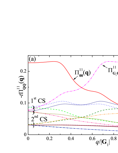
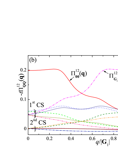
Figure 3: The components of the polarization operator $\Pi_{\mathbf{Q}\mathbf{Q}}^{11}(\mathbf{q})$ (a) and $\Pi_{\mathbf{Q}\mathbf{Q}}^{12}(\mathbf{q})$ (b) calculated in the SDW phase at $\mathbf{q}=q\bm{{\cal G}}_{1}/|\bm{{\cal G}}_{1}|$ for $\mathbf{Q}=0$ and $\mathbf{Q}$ belonging to the first two coordination spheres. The doping level is $n=-1.75$.

At small $\mathbf{q}+\mathbf{Q}$ one can obtain an analytical expression for the matrix $V_{\mathbf{Q}\mathbf{Q}^{\prime}}^{(0)isjs^{\prime}}$. In the case $i=j$, the translation symmetry allows us to convert the summation over ${\bf r}_{\mathbf{n}}^{is}$ to the summation over ${\bf r}_{\mathbf{n}}^{is}-{\bf r}_{\mathbf{m}}^{is}$, and the summation over $\mathbf{m}$ gives a factor $N_{sc}\delta_{\mathbf{QQ}^{\prime}}$ before the sum in Eq. (18). Further, when $\mathbf{q}+\mathbf{Q}$ is small ($|{\bf q}+{\bf Q}|\ll a^{-1}$), the lattice summation can be replaced by the space integration. As a result, we establish

$$V_{\mathbf{Q}\mathbf{Q}^{\prime}}^{(0)1s1s^{\prime}}(\mathbf{q})=V_{\mathbf{Q}\mathbf{Q}^{\prime}}^{(0)2s2s^{\prime}}(\mathbf{q})=\delta_{\mathbf{QQ}^{\prime}}\frac{2\pi e^{2}}{\epsilon v_{c}|\mathbf{q}+\mathbf{Q}|},$$ (19)

where $v_{c}=\sqrt{3}a^{2}/2$ is the area of the graphene unit cell. For $i\neq j$, one can find such $\mathbf{m}$ that $\mathbf{r}_{\mathbf{m}}^{2s^{\prime}}=d\mathbf{e}_{z}+\mathbf{r}_{\mathbf{n}}^{1s}+\bm{\delta}_{\mathbf{nm}}^{ss^{\prime}}$, where $\bm{\delta}_{\mathbf{nm}}^{ss^{\prime}}$ is small ($|\bm{\delta}_{\mathbf{nm}}^{ss^{\prime}}|\lesssim a$). At small $|{\bf q}+{\bf Q}|$ we can neglect $\bm{\delta}_{\mathbf{nm}}^{ss^{\prime}}$ and replace the summation by integration. This allows us to derive

$$V_{\mathbf{Q}\mathbf{Q}^{\prime}}^{(0)1s2s^{\prime}}(\mathbf{q})=V_{\mathbf{Q}\mathbf{Q}^{\prime}}^{(0)2s1s^{\prime}}(\mathbf{q})=\delta_{\mathbf{QQ}^{\prime}}\frac{2\pi e^{2}e^{-|\mathbf{q}+\mathbf{Q}|d}}{\epsilon v_{c}|\mathbf{q}+\mathbf{Q}|}.$$ (20)

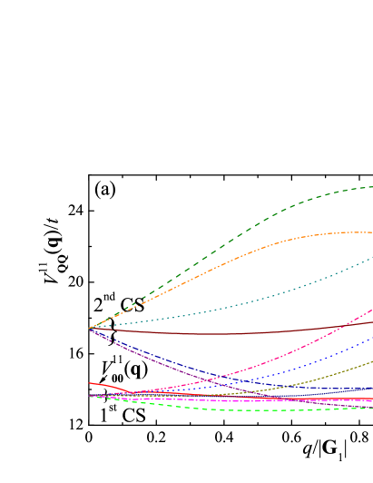
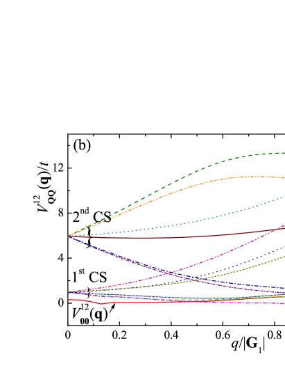
Figure 4: The dependence of renormalized Coulomb interaction $V_{\mathbf{Q}\mathbf{Q}}^{11}(\mathbf{q})$ (a) and $V_{\mathbf{Q}\mathbf{Q}}^{12}(\mathbf{q})$ (b) calculated in the SDW phase at $\mathbf{q}=q\bm{{\cal G}}_{1}/|\bm{{\cal G}}_{1}|$ for $\mathbf{Q}=0$ and for $\mathbf{Q}$ belonging to the first two coordination spheres. The doping level is $n=-1.75$ and $\epsilon=1$.

In our simulations, we use truncated matrices $\Pi_{\mathbf{Q}\mathbf{Q}^{\prime}}^{isjs^{\prime}}$ and $V_{\mathbf{Q}\mathbf{Q}^{\prime}}^{(0)isjs^{\prime}}$ with $\mathbf{Q}$ and $\mathbf{Q}^{\prime}$ being restricted to the insides of the eleventh coordination sphere (CS). The total number of such $\mathbf{Q}$ is $91$.

According to the expressions (19) and (20), the bare interaction $V_{\mathbf{Q}\mathbf{Q}^{\prime}}^{(0)isjs^{\prime}}$ at small transferred momentum is independent of the sublattice indices $s$, $s^{\prime}$. Then, one can prove that the screened interaction is also independent of these indices $V_{\mathbf{Q}\mathbf{Q}^{\prime}}^{isjs^{\prime}}=V_{\mathbf{Q}\mathbf{Q}^{\prime}}^{ij}$. The matrix $V_{\mathbf{Q}\mathbf{Q}^{\prime}}^{ij}$ satisfies Eq. (17) with the sublattice-independent polarization operator $\Pi_{\mathbf{Q}\mathbf{Q}^{\prime}}^{ij}$ defined as

$$\Pi_{\mathbf{Q}\mathbf{Q}^{\prime}}^{ij}=\sum_{ss^{\prime}}\Pi_{\mathbf{Q}\mathbf{Q}^{\prime}}^{isjs^{\prime}}.$$ (21)

We calculate the polarization operator numerically for different doping levels. The temperature is chosen as $T=5\times 10^{-3}W_{\text{SDW}}$, where $W_{\text{SDW}}$ is the width of the eight low-energy mean-field bands. It is not possible to perform the double summation in Eq. (16) over all bands at realistic time. For this reason we keep only $104$ bands closest to the Fermi level in the summation over $S$ and $S^{\prime}$, assuming that the contributions from higher energy bands are small. The functions $\Pi_{\mathbf{Q}\mathbf{Q}}^{11}(\mathbf{q})$ and $\Pi_{\mathbf{Q}\mathbf{Q}}^{12}(\mathbf{q})$ are shown in Fig. 3 for $\mathbf{Q}=0$ and for $\mathbf{Q}$ belonging to the first two CS. These results correspond to the doping level $n=-1.75$. The vector $\mathbf{q}$ is along the vector $\bm{{\cal G}}_{1}$. We see that $-\Pi_{\mathbf{00}}^{ij}(\mathbf{q})$ decreases with $\mathbf{q}$. The values of $-\Pi_{\mathbf{Q}\mathbf{Q}}^{ij}(\mathbf{0})$ decrease with the increase of the absolute values of $\mathbf{Q}$. Our simulations show that $\Pi_{\mathbf{Q}\mathbf{Q}^{\prime}}^{ij}(\mathbf{q})$ is almost diagonal in $\mathbf{Q}$ and $\mathbf{Q}^{\prime}$ for $\mathbf{Q}$ or $\mathbf{Q}^{\prime}$ belonging to the third and larger CS. In this case we have $\Pi_{\mathbf{Q}\mathbf{Q}^{\prime}}^{ij}(\mathbf{q})\cong\delta_{\mathbf{Q}\mathbf{Q}^{\prime}}\Pi_{\mathbf{Q}}^{ij}(\mathbf{q})$.

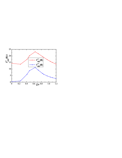
Figure 5: The dependence of $V_{\mathbf{Q}\mathbf{Q}}^{11}(\mathbf{0})$ (red triangles) and $V_{\mathbf{Q}\mathbf{Q}}^{12}(\mathbf{0})$ (blue circles) on $Q$. The doping level is $n=-1.75$ and $\epsilon=1$.

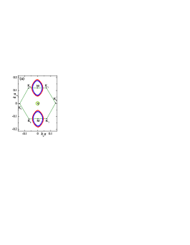
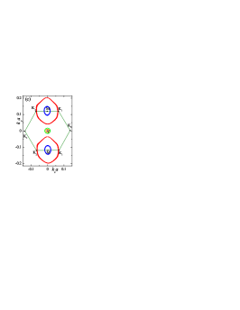
Figure 6: The Fermi surface in the SDW phase calculated for $n=-1.75$ (a), $n=-1.69$ (b), and $n=-1.67$ (c). For each doping there are two elliptical Fermi surface sheets centered at $\mathbf{M}$ point and two circular Fermi surface sheets centered at $\bm{\Gamma}$ point. In each plot the upper and lower $\mathbf{M}$ points are equivalent. Due to nematicity of the underlying spin texture, the Fermi surface symmetry is $C_{2}$, not $C_{6}$.

Figure 4 shows the dependence of the renormalized Coulomb interaction $V_{\mathbf{Q}\mathbf{Q}}^{11}(\mathbf{q})$ and $V_{\mathbf{Q}\mathbf{Q}}^{12}(\mathbf{q})$ on $q$ calculated for $\mathbf{Q}=0$ and for $\mathbf{Q}$ belonging to the first two CS. We see, that $V_{\mathbf{Q}\mathbf{Q}}^{ij}(\mathbf{0})$ increases with the increase of $Q$. Such a dependence exists up to the fourth CS. At larger $Q$, the $V_{\mathbf{Q}\mathbf{Q}}^{ij}(\mathbf{0})$ decreases approximately as $1/Q$. The dependence of $V_{\mathbf{Q}\mathbf{Q}}^{ij}(\mathbf{0})$ on $Q$ is shown in Fig. 5.

V Superconductivity

We examine a possibility of the superconducting state controlled by the renormalized Coulomb interaction near the half-filling, where it was observed experimentally Cao et al. (2018b); Lu et al. (2019). For each momentum $\mathbf{p}$ in the reduced Brillouin zone we arrange energies of the low-energy bands $E_{\mathbf{p}}^{({\cal S})}$ (${\cal S}=1,\,2,\dots,\,8$) in ascending order. In our study of the superconductivity we consider three doping levels: $n=-1.75$, $n=-1.69$, and $n=-1.67$.

In our scenario the superconductivity becomes possible since the SDW order cannot completely eliminate Fermi surface of MAtBLG. Thus, the remaining low-lying fermionic degrees of freedom can become unstable in the superconductivity channel. The Fermi surface structures corresponding to the three doping levels are shown in Fig. 6. For each doping there are two almost elliptical Fermi surface sheets centered at $\mathbf{M}$ point and two circular Fermi surface sheets centered at $\bm{\Gamma}$ point. Elliptical Fermi surfaces are formed by the bands with ${\cal S}_{1}=3$ (bigger ellipse) and ${\cal S}_{2}=4$ (smaller ellipse), while circular Fermi surface sheets are formed by the bands with ${\cal S}_{3}=1$ and ${\cal S}_{4}=2$. For $n=-1.75$ the sizes of ellipses are almost equal to each other, and when we increase the doping the sizes of the ellipses become more dissimilar. This happens because the low-energy spectra are almost doubly degenerate at half-filling, while the bands tend to separate from each other when $n$ approaches $-1$. Note that for the considered doping levels the mean-field spectra demonstrate nematicity, that is, the spectra have $C_{2}$ symmetry group, which is lower than the $C_{6}$ symmetry of the crystal. The nematic SDW order induces the nematicity of the Fermi surface, the latter is clearly visible in Fig. 6.

The bands ${\cal S}_{3}$ and ${\cal S}_{4}$ forming the circular Fermi surfaces are not interesting for the superconducting pairing since they have large Fermi velocities at the Fermi level and small Fermi momenta. The bands ${\cal S}_{1}$ and ${\cal S}_{2}$ forming the elliptical Fermi surfaces around $\mathbf{M}$ point are more relevant for the superconductivity since their Fermi velocities are small enough (the density of states is large) and the Fermi momenta are larger than that for the circular Fermi surfaces.

Using fermionic operators $\psi_{{\bf p}S}$ introduced in Eq. (14) and keeping only terms relevant for the superconducting pairing, one can rewrite the renormalized interaction Hamiltonian as follows

$$H_{\text{int}}=\frac{1}{2{\cal N}}\sum_{\mathbf{pp}^{\prime}}\sum_{\cal{SS}^{\prime}}\Gamma^{({\cal S},{\cal S}^{\prime})}_{\mathbf{pp}^{\prime}}\psi^{{\dagger}}_{-\mathbf{p}^{\prime}{\cal S}^{\prime}}\psi^{{\dagger}}_{\mathbf{p}^{\prime}{\cal S}^{\prime}}\psi^{\phantom{{\dagger}}}_{\mathbf{p}{\cal S}}\psi^{\phantom{{\dagger}}}_{-\mathbf{p}{\cal S}}\,.$$ (22)

Here and below the summation over ${\cal S}$ and ${\cal S}^{\prime}$ is performed over bands ${\cal S}_{1}$ and ${\cal S}_{2}$ and

$$\Gamma^{({\cal S},{\cal S}^{\prime})}_{\mathbf{pp}^{\prime}} = \!\!\!\sum_{ij\atop\mathbf{Q}_{1}\mathbf{Q_{2}}}\!\!\left(\sum_{\mathbf{G}s\sigma}\Phi_{\mathbf{pG}is\sigma}^{({\cal S})}\Phi_{\mathbf{p}^{\prime}\mathbf{G}+\mathbf{Q}_{1}is\sigma}^{({\cal S}^{\prime})*}\right)V^{ij}_{\mathbf{Q}_{1}\mathbf{Q}_{2}}(\mathbf{p}^{\prime}-\mathbf{p})$$ (23)

$$\times \!\!\!\left(\sum_{\mathbf{G}s\sigma}\Phi_{-\mathbf{pG}js\sigma}^{({\cal S})}\Phi_{-\mathbf{p}^{\prime}\mathbf{G}-\mathbf{Q}_{2}js\sigma}^{({\cal S}^{\prime})*}\right)$$

is the effective interaction in the Cooper channel.

We assume that in the superconducting state the following expectation values are non-zero

$$\eta^{({\cal S})}_{\mathbf{p}}=\left\langle\psi^{{\dagger}}_{-\mathbf{p}{\cal S}}\psi^{{\dagger}}_{\mathbf{p}{\cal S}}\right\rangle\,.$$ (24)

The total momentum of the pair is zero. We introduce the superconducting order parameter in the form

$$\Delta^{({\cal S})}_{\mathbf{p}}=\frac{1}{\cal N}\sum_{{\cal S}^{\prime}\mathbf{p}^{\prime}}\Gamma^{({\cal S},{\cal S}^{\prime})}_{\mathbf{pp}^{\prime}}\eta^{({\cal S}^{\prime})}_{\mathbf{p}^{\prime}}\,.$$ (25)

Transforming the interaction Hamiltonian (22) to its mean-field version, we derive the self-consistency equation for the order parameter. After standard calculations we obtain

$$\Delta^{({\cal S})}_{\mathbf{p}} = -\sum_{{\cal S}^{\prime}}\int\frac{d^{2}\mathbf{p}}{v_{\rm BZ}}\frac{\Gamma^{({\cal S},{\cal S}^{\prime})}_{\mathbf{pp}^{\prime}}\Delta^{({\cal S}^{\prime})}_{\mathbf{p}^{\prime}}}{2\sqrt{\left[E^{({\cal S}^{\prime})}_{\mathbf{p}^{\prime}}-\mu\right]^{2}+\left|\Delta^{({\cal S}^{\prime})}_{\mathbf{p}^{\prime}}\right|^{2}}}$$ (26)

$$\times \tanh\left[\frac{1}{2T}\sqrt{\left[E^{({\cal S}^{\prime})}_{\mathbf{p}^{\prime}}-\mu\right]^{2}+\left|\Delta^{({\cal S}^{\prime})}_{\mathbf{p}^{\prime}}\right|^{2}}\right]\,,$$

where $v_{\rm BZ}$ is the Brillouin zone area of the graphene and the integration is performed over the reduced Brillouin zone.

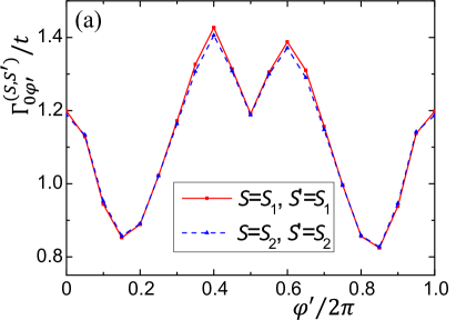
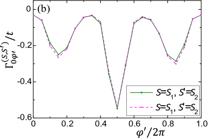
Figure 7: Interaction in the Cooper channel. The dependence of $\tilde{\Gamma}^{({\cal S},{\cal S}^{\prime})}_{0\varphi^{\prime}}$ on $\varphi^{\prime}$, calculated for $n=-1.75$. Panel (a) corresponds to ${\cal S}={\cal S}_{1},\,{\cal S}^{\prime}={\cal S}_{1}$ and ${\cal S}={\cal S}_{2},\,{\cal S}^{\prime}={\cal S}_{2}$, while panel (b) corresponds to ${\cal S}={\cal S}_{1},\,{\cal S}^{\prime}={\cal S}_{2}$ and ${\cal S}={\cal S}_{2},\,{\cal S}^{\prime}={\cal S}_{1}$, see the legend.

We do not solve the integral equation (26), but only estimate the critical temperature $T_{c}$ by order of magnitude. With a good accuracy the Fermi surface sheets centered at $\mathbf{M}$ point have shapes of ellipses. One can introduce the polar angle $\varphi$ and parameterize the Fermi momenta of the bands ${\cal S}_{1}$ and ${\cal S}_{2}$ as $\mathbf{p}_{\rm F}^{({\cal S})}(\varphi)=\mathbf{M}+\mathbf{k}_{\rm F}^{({\cal S})}(\varphi)$, where

$$\mathbf{k}_{\rm F}^{({\cal S})}(\varphi)=k_{1F}^{({\cal S})}\mathbf{n}_{1}\cos\varphi+k_{2F}^{({\cal S})}\mathbf{n}_{2}\sin\varphi\,.$$ (27)

In this equation, $k_{1F}^{({\cal S})}$ and $k_{2F}^{({\cal S})}$ are found by fitting of the ${\cal S}$’th Fermi surface sheet by an ellipse, and $\mathbf{n}_{1}$ and $\mathbf{n}_{2}$ are the unit vectors parallel and perpendicular to the vector $\bm{{\cal G}}_{2}$, correspondingly. Near the ${\cal S}$’th Fermi surface sheet, one can write the energy of the band ${\cal S}$ as

$$E_{\mathbf{M}+\mathbf{k}}^{({\cal S})}\cong\mu+\mathbf{v}^{({\cal S})}(\varphi)\cdot\left[\mathbf{k}-\mathbf{k}_{\rm F}^{({\cal S})}(\varphi)\right],$$ (28)

where

$$\mathbf{v}^{({\cal S})}(\varphi)=\left.\frac{\partial E_{\mathbf{M}+\mathbf{k}}^{({\cal S})}}{\partial\mathbf{k}}\right|_{\mathbf{k}=\mathbf{k}_{\rm F}^{({\cal S})}(\varphi)}\,.$$ (29)

In Eq. (26), we introduce for each ${\cal S}^{\prime}$ the polar coordinates $(k,\,\varphi)$ in the integral over $\mathbf{p}$ as follows

$$\mathbf{p}=\mathbf{M}+k\left(\mathbf{n}_{1}\cos\varphi+\varkappa^{({\cal S})}\mathbf{n}_{2}\sin\varphi\right),$$ (30)

where $\varkappa^{({\cal S})}=k_{2F}^{({\cal S})}/k_{1F}^{({\cal S})}$. In this case, we have $d^{2}\mathbf{p}=\varkappa^{({\cal S})}kdkd\varphi$. Using Eqs. (27) and (30) we can rewrite Eq. (28) in the form

$$E_{\mathbf{M}+\mathbf{k}}^{({\cal S})}\cong\mu+\tilde{v}^{({\cal S})}(\varphi)\left(k-k_{1F}^{({\cal S})}\right),$$ (31)

where

$$\tilde{v}^{({\cal S})}(\varphi)=\mathbf{v}^{({\cal S})}(\varphi)\cdot\left(\mathbf{n}_{1}\cos\varphi+\varkappa^{({\cal S})}\mathbf{n}_{2}\sin\varphi\right).$$ (32)

We replace $\Gamma^{({\cal S},{\cal S}^{\prime})}_{\mathbf{pp}^{\prime}}$ in Eq. (26) by their values at Fermi momenta introducing the functions

$$\tilde{\Gamma}^{({\cal S},{\cal S}^{\prime})}_{\varphi\varphi^{\prime}}=\Gamma^{({\cal S},{\cal S}^{\prime})}_{{\bf p}{\bf p}^{\prime}}\Big{|}_{{{\bf p}=\mathbf{M}+\mathbf{k}_{\rm F}^{({\cal S})}(\varphi)\atop{\bf p}^{\prime}=\mathbf{M}+\mathbf{k}_{\rm F}^{({\cal S}^{\prime})}(\varphi^{\prime})}}\,.$$ (33)

Finally, we assume the following ansatz for the superconducting order parameter

$$\Delta^{({\cal S})}_{\mathbf{M}+\mathbf{k}}=\left\{\begin{array}[]{cl}\Delta^{({\cal S})}(\varphi)\,,&\;\;\tilde{v}^{({\cal S})}(\varphi)\left|k-k_{1F}^{({\cal S})}\right|<\varepsilon_{0},\\ 0\,,&\;\;\text{otherwise}\,,\end{array}\right.$$ (34)

where $\varepsilon_{0}\sim W_{\rm SDW}$ is the cutoff energy. In the limit of $T\to T_{c}$ one can linearize the equation for the superconducting order parameter taking $\Delta^{({\cal S}^{\prime})}_{\mathbf{p}^{\prime}}=0$ in the square roots in the integrals in Eq. (26). Keeping in mind all aforementioned formulas and taking the integral over $k$ in the limit $\varepsilon_{0}/T\gg 1$, we obtain the equations for $\Delta^{({\cal S})}(\varphi)$ in the form

$$\Delta^{({\cal S})}(\varphi)=-\sum_{{\cal S}^{\prime}}\int\limits_{0}^{2\pi}d\varphi^{\prime}\frac{\tilde{\Gamma}^{({\cal S},{\cal S}^{\prime})}_{\varphi\varphi^{\prime}}k_{2F}^{({\cal S}^{\prime})}\Delta^{({\cal S}^{\prime})}(\varphi^{\prime})}{v_{\rm BZ}|\tilde{v}^{({\cal S}^{\prime})}(\varphi^{\prime})|}\ln\frac{E^{*}}{T}\,,$$ (35)

where $E^{*}=\varepsilon_{0}/(2A)$ and $\ln A=\ln\pi/4-C$ ($C$ is the Euler’s constant, $A\cong 0.441$).

We calculate the functions $\tilde{\Gamma}^{({\cal S},{\cal S}^{\prime})}_{\varphi\varphi^{\prime}}$ in Eq. (33) numerically. An appropriate choose of the phase of the wave functions $\Phi_{\mathbf{pG}is\sigma}^{({\cal S})}$ makes $\tilde{\Gamma}^{({\cal S},{\cal S}^{\prime})}_{\varphi\varphi^{\prime}}$ real. The dependence of $\tilde{\Gamma}^{({\cal S},{\cal S}^{\prime})}_{0\varphi^{\prime}}$ on $\varphi^{\prime}$ calculated for $n=-1.75$ is shown in Fig. 7. We see that the absolute value of $\tilde{\Gamma}^{({\cal S},{\cal S}^{\prime})}_{0\varphi^{\prime}}$ have maxima at $\varphi^{\prime}=\pi$ if ${\cal S}\neq{\cal S}^{\prime}$, see panel (b). The maxima of $\tilde{\Gamma}^{({\cal S},{\cal S}^{\prime})}_{0\varphi^{\prime}}$ for ${\cal S}={\cal S}^{\prime}$ are located near the $\varphi^{\prime}=\pi$, panel (a). When $\varphi\neq 0$, the functions $\tilde{\Gamma}^{({\cal S},{\cal S}^{\prime})}_{\varphi\varphi^{\prime}}$ have maxima at $\varphi^{\prime}\approx\varphi+\pi$. Such a behavior of $\tilde{\Gamma}^{({\cal S},{\cal S}^{\prime})}_{\varphi\varphi^{\prime}}$ can stabilize the superconducting state just due to the electron repulsion. To show this, let us choose the trial function for $\Delta^{({\cal S})}(\varphi)$ in the form $\Delta^{({\cal S})}(\varphi)=\Delta^{({\cal S})}_{0}\cos\varphi$. Multiplying both sides of Eq. (35) by $2\cos\varphi$ and integrating over $\varphi$ one obtains the equation for $\Delta^{({\cal S})}_{0}$:

$$\Delta^{({\cal S})}_{0}=\sum_{{\cal S}^{\prime}}\lambda^{({\cal S},{\cal S}^{\prime})}\Delta^{({\cal S}^{\prime})}_{0}\ln\frac{E^{*}}{T}\,,$$ (36)

where

$$\lambda^{({\cal S},{\cal S}^{\prime})}=-\frac{a^{2}\sqrt{3}k_{2F}^{({\cal S}^{\prime})}}{2\pi}\!\!\int\limits_{0}^{2\pi}\!\!\frac{d\varphi}{2\pi}\!\!\int\limits_{0}^{2\pi}\!\!\frac{d\varphi^{\prime}}{2\pi}\frac{\tilde{\Gamma}^{({\cal S},{\cal S}^{\prime})}_{\varphi\varphi^{\prime}}\cos\varphi\cos\varphi^{\prime}}{|\tilde{v}^{({\cal S}^{\prime})}(\varphi^{\prime})|}\,.$$ (37)

The most important is that the double integral in Eq. (37) is negative for ${\cal S}={\cal S}^{\prime}$ and $\lambda^{({\cal S},{\cal S})}>0$ due to the properties of $\tilde{\Gamma}^{({\cal S},{\cal S}^{\prime})}_{\varphi\varphi^{\prime}}$ described above. As a result, Eq. (36) has non-trivial solutions for two values of $T$, the maximum of these two temperatures corresponds to $T_{c}$. The result can be presented in the form

$$T_{c}=E^{*}e^{-1/\Lambda},$$ (38)

where

$$\Lambda\!=\!\frac{\left[\lambda^{(3,3)}+\lambda^{(4,4)}+\sqrt{[\lambda^{(3,3)}-\lambda^{(4,4)}]^{2}+4\lambda^{(3,4)}\lambda^{(4,3)}}\right]}{2}.$$ (39)

We calculate $\Lambda$ numerically for three doping levels corresponding to the Fermi surfaces shown in Fig. 6. For $n=-1.75$, $n=-1.69$, and $n=-1.67$ we obtain, respectively, $\Lambda=0.05$, $\Lambda=0.09$, and $\Lambda=0.08$. Thus, the maximum $T_{c}$ corresponds to $n=-1.69$, Fig. 6(b). Taking for estimate $E^{*}=W_{\text{SDW}}\cong 17$ meV, we obtain in the latter case $T_{c}\cong 2.6$ mK. This value is much smaller than the experimentally observed Cao et al. (2018b); Lu et al. (2019) $T_{c}\approx 1.7$ K. Thus, the considered Coulomb interaction alone is not enough to stabilize the superconducting state with experimentally observed critical temperature. The implications of this finding are discussed below.

VI Discussion and Conclusions

In this paper we consider a possibility of superconducting phase in MAtBLG, and, more specifically, a Coulomb-interaction-driven superconducting mechanism in MAtBLG. At the center of our proposal is the notion that at least some parts of the MAtBLG Fermi surface remain ungapped despite the SDW order parameter presence. The fermionic degrees of freedom that remain at the Fermi energy even after the emergence of the SDW order is a peculiar feature of MAtBLG Sboychakov et al. (2019); Sboychakov et al. (2020a); Sboychakov et al. (2022). The residual Fermi surface can host a weaker order parameter, such as a superconductivity. This is the most important theoretical point of our proposal. This scenario has three obvious consequences, which can be tested in experiment. (i) The superconductivity coexists with the (stronger) SDW phase, (ii) the superconducting order parameter is unavoidably nematic, thanks to the nematicity of the underlying SDW order parameter, and (iii) our proposal entails large coherence length $\xi$: the usual BCS estimate $\xi=v_{\rm F}/\Delta\sim LW_{\rm SDW}/\Delta$ suggests that $\xi$ greatly exceeds the moiré period $L$, which itself is significant, due to large ratio $W_{\rm SDW}/\Delta$. Note also that, due to (i) and (ii), a familiar classification of superconducting order parameters into $s$-, $p$-, and $d$-wave symmetry classes is impossible.

Besides the presence of the Fermi surface, an essential ingredient of a mechanism is a source of attraction keeping Cooper pairs together. In the previous section we attempted to assess to which extent the renormalized Coulomb interaction can serve this purpose. Our calculations revealed that the resultant critical temperature is much lower than the value observed in the experiment.

Clearly, the discrepancy in terms of $T_{c}$ requires additional analysis. It is easy to convince oneself that the root cause of the superconducting instability weakness is is the weakness of the coupling constant $\Lambda$. In our estimates $\Lambda$ never exceeded 0.1, making the BCS exponent $\exp(-1/\Lambda)$ extremely small.

Moreover, in the regime of small $\Lambda$, any inaccuracy in $\Lambda$ is greatly amplified by the BCS exponential function. To illustrate this sensitivity in our circumstances, let us increase the coupling constant two-fold, from 0.09 to 0.18. Then the critical temperature grows by more than two orders of magnitude, from 2.6 mK to 0.66 K, which compares favorably against 1.7 K measured experimentally. This simple calculation reminds us that an order-of-magnitude estimate of $\Lambda$ is insufficient for an order-of-magnitude estimate of $T_{c}$. This issue is particularly pressing in the limit of low $\Lambda$, as in our case.

We envision two possibilities that can reconcile the theory with the experiment. One option is simply to resign to the fact that approximate nature of our calculations limits us to order-of-magnitude estimate $\Lambda$, which is equivalent to order-of-magnitude estimate of $\ln T_{c}$. We should not consider this viewpoint as excessively defeatist. After all, any many-body calculation is performed under numerous assumptions that skew the final answer. For MAtBLG the situation is worsen by lack of reliable knowledge about the interlayer tunneling.

Alternatively, we can add phonons to our mechanism. One can imagine two possibilities for phonon-mediated attraction. (i) The phonons increase the coupling constant $\Lambda$ discussed in the previous section, increasing the critical temperature. (ii) On the other hand, the phonon-mediated attraction may stabilize a superconducting order parameter of different type (e.g., node-less). In the latter case, the competition between two (or more) order parameters of different structures becomes a possibility.

Finally, when interpreting experimental data for MAtBLG, one needs to remember that the system might experience electronic phase separation. For twisted bilayer graphene this phenomenon has been discussed in Ref. Sboychakov et al., 2020b, but it itself is not uncommon in theoretical models for doped SDW phase Gorbatsevich et al. (1992); Igoshev et al. (2010); Sboychakov et al. (2013b, c, a); Rakhmanov et al. (2017, 2013, 2020); Kokanova et al. (2021), as well as for other continuous phase transitions affected by doping Fine and Egami (2008). Phase separation frustrated by long-range Coulomb interaction may lead to spatial pattern formation altering transport Narayanan et al. (2014) and other physical properties of a sample.

In conclusion, we argued that MAtBLG can enter a superconducting phase coexisting with the SDW-like ordering. The mean field description of the host SDW state accounts for on-site, and both in-plane and out-of-plane nearest-neighbor intersite anomalous expectation values. Numerical mean field minimization reveals that the SDW order leaves small multi-component Fermi surface ungapped. Near the half-filling the SDW order parameters partially break the MAtBLG point symmetry group that leads to the Fermi surface nematicity. For superconductivity the presence of the ungapped Fermi surface is crucial as it bypasses the competition between the magnetic and superconducting phases, which the (much weaker) superconductivity cannot win. Additionally, we explore the possibility of purely Coulomb-based mechanism of the superconductivity in MAtBLG. The screened Coulomb interaction is calculated within the random phase approximation. We show that near the half-filling the renormalized Coulomb repulsion indeed stabilizes the superconducting state. The superconducting order parameter has two nodes on the Fermi surface. We estimate the superconducting transition temperature and discuss the implications of our proposal.