An Edge-based Interface Tracking (EBIT) Method for Multiphase-flows Simulation with Surface Tension

Abstract

We present a novel Front-Tracking method, the Edge-Based Interface Tracking (EBIT) method for multiphase flow simulations. In the EBIT method, the markers are located on the grid edges and the interface can be reconstructed without storing the connectivity of the markers. This feature makes the process of marker addition or removal easier than in the traditional Front-Tracking method. The EBIT method also allows almost automatic parallelization due to the lack of explicit connectivity.

In a previous journal article we have presented the kinematic part of the EBIT method, that includes the algorithms for interface linear reconstruction and advection. Here, we complete the presentation of the EBIT method and combine the kinematic algorithm with a Navier–Stokes solver. To identify the reference phase and to distinguish ambiguous topological configurations, we introduce a new feature: the Color Vertex. For the coupling with the Navier–Stokes equations, we first calculate volume fractions from the position of the markers and the Color Vertex, then viscosity and density fields from the computed volume fractions and finally surface tension stresses with the Height-Function method. In addition, an automatic topology change algorithm is implemented into the EBIT method, making it possible the simulation of more complex flows. A two-dimensional version of the EBIT method has been implemented in the open-source Basilisk platform, and validated with five standard test cases: (1) translation with uniform velocity, (2) single vortex, (3) capillary wave, (4) Rayleigh-Taylor instability and (5) rising bubble. The results are compared with those obtained with the Volume-of-Fluid (VOF) method already implemented in Basilisk.

1 Introduction

Multiphase flows are ubiquitous in nature and engineering, and their numerical simulation still represents a formidable challenge, especially when a wide range of scales is involved, as in breaking waves on the sea surface, in some industrial processes or in atomizing liquid jets. Scales from meters to microns are typically seen. Large Reynolds number turbulence, as well as mass and heat transfers are the main causes for the introduction of such a wide range of scales. The CO₂ transfer and heat exchange between the oceans and the atmosphere is tightly linked to multiphase flows, as it takes place through the production and dispersion of small bubbles and droplets. Similar small structures are observed in technology, for example in the heat exchange and transport in nuclear reactors, the atomization of liquids in combustion and other settings, and in most of the synthesis processes in chemical engineering. For many of these natural and engineering problems, numerical modelling is extremely desirable, albeit a monumental challenge.

However, in the general area of multiphase flow simulation, much progress has recently been achieved in the interrelated issues of multiple scales, discretization, and topology change. These issues are: i) the long-standing one of how to represent numerically (i.e., simulate) a dynamic or moving curve or surface, ii) the more difficult or challenging problem of how to efficiently model and discretize problems at multiple scales, and finally iii) the still open issue of how to take advantage of hierarchical data structures and grids, such as quadtrees and octrees, to address the “tyranny of small scales” [1].

The first, moving curve issue is divided into two problems: the kinematic problem, where the motion of the curve or surface separating the phases must be described by knowing the fluid velocity field and the rate of phase change, and the dynamic problem, where the momentum and energy conservation equations must be solved for given fluid properties. Methods available for the kinematic problem are sometimes separated into Front-Capturing and Front-Tracking methods. In the first kind, Front-Capturing methods, a tracer or marker function $f({\bf x},t)$ is integrated in time with the knowledge of an adequate velocity field ${\bf u}({\bf x},t)$

$$\partial_{t}f+{\bf u}\cdot\nabla f=0$$ (1)

The tracer function can be a Heaviside function, leading to Volume-of-Fluid (VOF) methods [2, 3] or a smooth function, leading to Level-Set (LS) methods [4, 5].

In Front-Tracking methods, the interface or “front” is represented by a curve discretization, for example a spline, which evolves with a prescribed normal velocity $V_{S}$ , see [6]. Compatibility between the two formulations is achieved if ${\bf u}\cdot{\bf n}=V_{S}$. An introduction to the most popular methods may be found in [7]. Another point of view on the methods, that is fruitful in connection with issues ii) and iii) above, can be obtained by investigating how the data structures are tied to the underlying Eulerian grid. The data structures are local when their components have little or no “knowledge” of the overall connections among pieces of interface or connected regions of a given phase (Fig. 1b). Thus a discretization of the tracer function $f$ is a local data structure, tied to the Eulerian grid. On the other hand a global data structure contains information not only about individual points on the interface, but also about their connections with the entire interface of a given object. For Front-Tracking methods this is achieved by linked lists, or pointers, that allow to navigate the data structure along the object (Fig. 1a). It is then obvious and efficient, using the data structure, to find all the connected pieces of the interface.

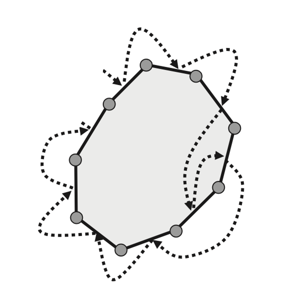
(a)	(b)

Figure 1: (a) A global data structure with a linked list: the example of the front. Reproduced from [7]. (b) A local data structure with unlinked VOF linear reconstructions.

The local data structures are not limited to VOF or LS methods. For example, an unconnected marker or particle method, such as Smoothed Particle Hydrodynamics (SPH), or other methods, simply tracks particles of position ${\bf x}_{i}$ by integrating

$$\frac{{\rm d}{\bf x}_{i}}{{\rm d}t}={\bf u}({\bf x}_{i},t)$$ (2)

without any concept of connection between the particles [8]. Such an unconnected marker method, despite its similarity with Front-Tracking is in fact a local method. Both the local and the global approaches have advantages. The local methods are easy to parallelize on a grid, are free of constraints that require the solutions of large linear or nonlinear systems (as when constructing interfaces by high-order splines) and are generally computationally efficient. The global methods allow to track and control the topology, so they are also useful for the second issue, the handling of multiscale problems. Moreover, when dealing with complex multiscale problems, it is often useful to investigate geometrical properties such as skeletons [9] which are branched manifolds most naturally represented by Front-Tracking. Global methods also allow to naturally distinguish between continuous slender objects such as unbroken thin ligaments or threads and strings of small particles or broken ligaments. This latter distinction is of great importance when analyzing statistically highly-fragmented flows [10]. It is however possible to represent slender objects with local methods in some cases: Chiodi [11] proposed an enhancement of the VOF interface reconstruction method, involving two nearly parallel, closely located planes in three dimensions, in order to capture slender sheets thinner than the mesh size.

A method that combines some of the properties of global methods, such as Front-Tracking, and local methods, such as VOF or LS, seems desirable. There have indeed been some prior attempts at such a combination.

Aulisa et al.[12, 13] combined the VOF method with marker points to obtain smooth interfaces without discontinuity and to improve mass conservation of traditional Front-Tracking methods. López et al. [14] introduced the marker points into the VOF method to allow tracking fluid structures thinner than the cell size.

The Level Contour Reconstruction Method (LCRM) developed by Shin, Juric and collaborators [15, 16, 17] combined Front-Tracking and LS methods. It improved the mass conservation problem of traditional LS methods, thanks to tracking the interface by Lagrangian elements (instead of advecting the LS function field). A LS function can then be regenerated from the Lagrangian elements. The smoothing of interface elements, as well as topology changes, take place automatically during the reconstruction procedure, thus explicit connectivity information is not needed in their method. Singh and Shyy [18] used the LCRM to perform topology changes in their traditional Front-Tracking method where connectivity of the Lagrangian elements has to be maintained explicitly. Shin, Yoon and Juric[19] later extended the LCRM to obtain a new type of Front-Tracking method, the Local Front Reconstruction Method (LFRM), for both two-dimensional and three-dimensional multiphase flow simulations. The LFRM reconstructs interface elements using the geometrical information directly from the Lagrangian interface elements instead of constructing another LS field.

We suggest a similar method in the present work, based on a purely kinematic approach developed by two of us [20], called the Edge-Based Interface-Tracking (EBIT) method. In that method the position of the interface is tracked by marker points located on the edges of an Eulerian grid, and the connectivity information is implicit. The basic idea and the split interface advection were discussed in [20], here we improve the mass conservation of the original EBIT method by using a circle fit to reconstruct the interface during advection. The topology change mechanism is also introduced. Compared to the LFRM of Shin, Yoon and Juric [19], markers in the EBIT method are bound to the Eulerian grid. These marker are obtained by a reconstruction of the interface at every time step, thus the Eulerian grid and Lagrangian markers can be distributed to different processors by the same routine as the one used in the parallelization of the Navier–Stokes solver. Second, a new feature called Color Vertex, which amounts to describe the topology of the interface by the color of markers at the vertices of the grid, is discussed. Such a scheme is trivial on a simplex and just slightly more complicated on a square grid. It was proposed in a similar context by Singh and Shyy [18]. Third, we combine the EBIT method with a Navier–Stokes solver for multiphase flow simulations. The coupling is simply realized by computing volume fractions from the position of the markers and the Color Vertex, then we use the volume fractions as in typical VOF solvers [7].

The paper is organized as follows: the kinematics of the EBIT method is described in Section 2. This includes the interface advection algorithm, the updating rules for the color vertices and the automatic topology change algorithm. Then the coupling algorithm between the EBIT interface description and the multiphase fluid dynamics is presented. A two-dimensional flow solver based on a Cartesian or quadtree grid is implemented inside the open-source platform Basilisk [21, 22]. In Section 3, the EBIT method is validated by the computation of typical examples of multiphase flow simulations. The results obtained by the combined EBIT and VOF methods are presented and compared with those calculated by the pure VOF method.

2 Numerical method

2.1 The EBIT method

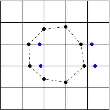
(a)	(b)
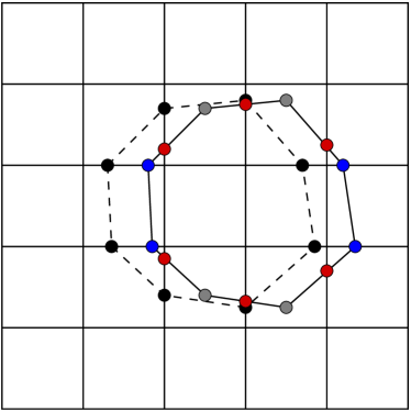
(c)	(d)

Figure 2: One-dimensional advection of the EBIT method along the $x$-axis. (a) Initial interface line. (b) Advection of the markers on the grid lines aligned with the velocity component (blue points). (c) Advection of the unaligned markers (gray points) and computation of the intersections with the grid lines (red points). (d) Interface line after the 1D advection.

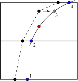
Figure 3: Circle fit to compute the position of the unaligned marker (red point)

In the EBIT method, the interface is represented by a set of marker points placed on the grid lines. The advection of the interface is done by moving these points along the grid lines. The equation of motion for a marker point at position ${\bf x}_{i}$ is

$$\frac{d\boldsymbol{x}_{i}}{dt}=\boldsymbol{u}_{i}$$ (3)

which is discretized by a first-order explicit Euler method

$$\boldsymbol{x}^{n+1}_{i}=\boldsymbol{x}^{n}_{i}+\boldsymbol{u}^{n}_{i}\Delta t$$ (4)

where the velocity ${\bf u}^{n}_{i}$ at the marker position ${\bf x}^{n}_{i}$ is calculated by a bilinear interpolation.

For a multi-dimensional problem, a split method is used to advect the interface (see Fig. 2), which is similar to that described in [20], but with some improvements. The marker points placed on the grid lines that are aligned with the velocity component of the 1D advection are called aligned markers, while the remaining ones are called unaligned markers. Starting from the initial position at time step $n$, the new position of the aligned markers is obtained by Eq. (4) (blue points of Fig. 3). To compute the new unaligned markers, we first advect them using again Eq. (4), obtaining in this way the gray point of Fig. 3c. Finally, the new position of the unaligned marker (red point of Fig. 3d) is obtained by fitting a circle through the surrounding marker points and by computing the intersection with the corresponding grid line. The gray point is then discarded. Whenever it is possible, we consider two circles for the fitting, through points 2,3,4 and 1,2,3 of Fig. 3, respectively. In that case, the final position of the unaligned marker will be the average of the two fits.

2.2 Color Vertex

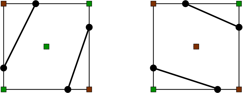
Figure 4: Two color vertex configurations (brown and green squares) to select a different connectivity in the same set of markers

In the EBIT method, the connectivity of the markers is implicit. When there are only two markers on the cell boundary, the interface portion is given by the segment connecting these two points. However, when there are four markers on the boundary, there are two possible alternative configurations, as shown in Fig. 4. In order to select one of the two configurations without any ambiguity, we consider a technique called Color Vertex, which was first proposed by Singh and Shyy [18] to implement an automatic topology change. The value of the Color Vertex indicates the fluid phase in the corresponding region within the cell, and five color vertices (four in the corners and one in the center of the cell) are enough to select one of the two configurations of Fig. 4. In other word, we can establish a one-to-one correspondence between the topological configuration and the value of the color vertices within each cell, and then reconstruct the interface segments with no ambiguity.

Furthermore, the direction of the unit normal to the interface can also be determined based on the Color Vertex distribution. The local feature of the Color Vertex makes the EBIT method more suitable for parallelization, when it is compared to the data structure that is used for storing the connectivity in traditional Front-Tracking methods.

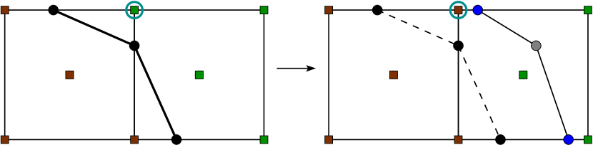
Figure 5: Update of the Color Vertex value on a cell corner: its value changes, from green to brown, as the marker is advected across the grid lines intersection

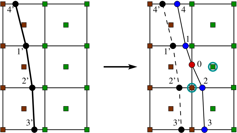
(a)

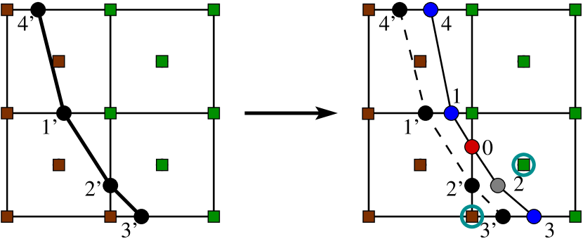
(b)

Figure 6: Update of the Color Vertex value in the cell center with an unaligned marker (red point)

As the interface is advected, the value of a Color Vertex should also be updated accordingly to ensure that the implicit connectivity information is retained. For a Color Vertex located on a cell corner, we have to change its value if a marker moves across the intersection of the corresponding grid lines, as shown in Fig. 5.

In the present implementation of the EBIT algorithm the Color Vertex in the cell center is only used to select one of the two configurations shown in Fig. 4. It is important to realize that in such a configuration, regardless of the direction of the advection, there are both aligned markers and unaligned ones. Therefore, the algorithm for updating the Color Vertex in the cell center proceeds as follows (see Fig. 6):

(1) If in the cell under investigation, after the interface advection there is an unaligned marker (red point 0 of Fig. 6), we identify the interface segment through points 1 and 2 that brackets the unaligned marker and the corresponding segment through points 1’ and 2’, before the advection step. These two points are on opposite sides in Fig. 6(a) and on consecutive sides in Fig. 6(b).

(2) From the connectivity information before the advection step, we identify two more markers, points 3’ and 4’, that are connected to the segment 1’-2’ on opposite sides, and compute their new positions 3 and 4 after the advection step.

(3) If the four points 1, 2, 3 and 4 are unaligned markers, we do not need to update the value of the Color Vertex in the center, because in this case it is impossible to have an ambiguous configuration.

(4) We check if in the cell under investigation there is an aligned marker (point 2 in Fig. 6(a) and point 3 in Fig. 6(b)).

(5) If an aligned marker has been found, we identify the cell corner (bottom left corner of Fig. 6) isolated by the segments connecting this marker and the new unaligned marker (point 0 of Fig. 6). The value of the Color Vertex in the cell center is set to the opposite value of that of the cell corner.

With these simple rules, the value of the Color Vertex in the cell center is set to the correct value to select one of the two configurations of Fig. 4.

2.3 Topology change

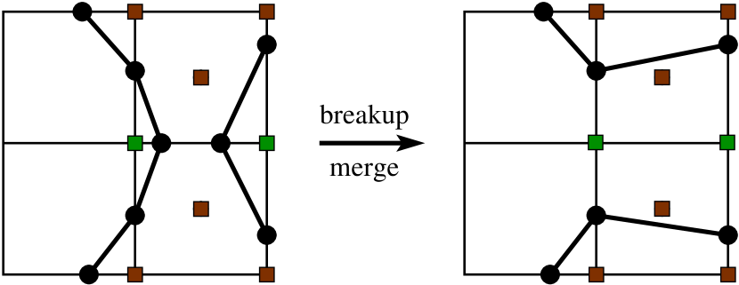
Figure 7: Topology change mechanism

The topology change is controlled by the Color Vertex value distribution in an automatic manner. In the present implementation of the EBIT method, a marker point is present on a cell edge only if the value of the Color Vertex at the two edge endpoints is different.

Furthermore, only one marker is allowed on a cell edge. When two markers move into the same edge, as shown in Fig. 7, they both will be eliminated automatically, because the value of the Color Vertex at the corresponding endpoints is the same, hence there cannot be any marker on that edge. Moreover, the “surviving” markers within the cell will be reconnected automatically, see again Fig. 7. This reconnection procedure enables ligament breakup or droplet merging in an automatic way during the interface advection. As a direct consequence of this procedure, the volume occupied by the reference phase will decrease or increase. In particular, it tends to remove droplets or bubbles which are smaller than the grid size.

This topology change mechanism only affects interfaces that are approaching each other along a direction parallel to the grid lines. Because of the presence of a Color Vertex in the cell center, interfaces approaching along a diagonal direction do not induce any topology change, as long as the four markers remain on a different edge, as shown in Fig. 4. Thus, this mechanism does not suffer the problem of orientation-dependent topology change, which takes place during the tetra-marching procedure in Yoon’s [23] LCRM and Shin’s [19] LFRM, along the two diagonal directions.

However, in our method approaching interfaces along diagonal directions behave differently from those approaching along parallel ones. A possible solution to this problem would be removing the restriction on the number of markers per edge, which would also allow us to capture the subscale interfacial structure and to control the topology change based on a physical mechanism.

2.4 Governing equations

The Navier–Stokes equations for incompressible two-phase flow with immiscible fluids written in the one-fluid formulation are

$$\frac{\partial\rho}{\partial t}+\boldsymbol{u}\cdot\nabla\rho=0$$ (5)

$$\frac{\partial\rho\boldsymbol{u}}{\partial t}+\nabla\cdot(\rho\boldsymbol{u}\boldsymbol{u})=-\nabla p+\nabla\cdot\left[\mu\left(\nabla\boldsymbol{u}+\nabla\boldsymbol{u}^{T}\right)\right]+\rho\boldsymbol{g}+\boldsymbol{f}$$ (6)

$$\nabla\cdot\boldsymbol{u}=0$$ (7)

where $\rho$ and $\mu$ are density and viscosity, respectively. The gravitational force is taken into account with the $\rho\boldsymbol{g}$ term. Surface tension is modeled by the term $\boldsymbol{f}=\sigma\kappa\boldsymbol{n}\delta_{S}$, where $\sigma$ is the surface tension coefficient, $\kappa$ the interface curvature, $\boldsymbol{n}$ the unit normal and $\delta_{S}$ the surface Dirac delta function.

The physical properties are calculated as

$$\rho=H\rho_{1}+(1-H)\rho_{2},\qquad\mu=H\mu_{1}+(1-H)\mu_{2}$$ (8)

where $H$ is the Heaviside function, which is equal to 1 inside the reference phase and 0 elsewhere.

Since the markers are located on the grid edges, we consider a simple strategy to couple the EBIT method with the Navier–Stokes equations. From the position of the marker points and the values of Color Vertex in the cell under investigation, we can easily compute the equation of the straight line connecting the markers and the volume fraction $C$ [24]. The volume fraction field is then used to approximate the Heaviside function in Eq. (8) and to calculate the curvature by the generalized height function method [22] and the Dirac delta function in Eq. (6).

The numerical implementation of the EBIT method has been written in the Basilisk C language [21, 22], which adopts a time-staggered approximate projection method to solve the incompressible Navier–Stokes equations on a Cartesian mesh or a quad/octree mesh. The Bell-Colella-Glaz (BCG) [25] second-order scheme is used to discretize the advection term, and a fully implicit scheme for the diffusion term. A well-balanced Continuous Surface Force (CSF) method is used to calculate the surface tension term [22, 26].

2.5 Adaptive mesh refinement (AMR)

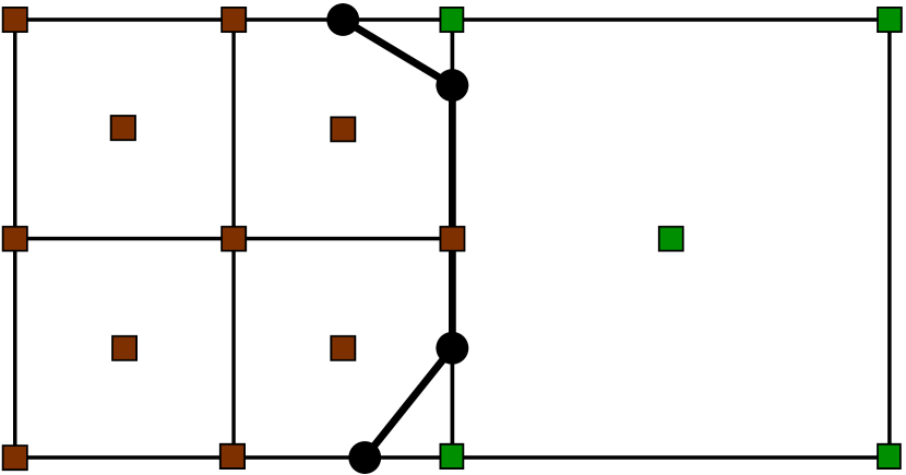
Figure 8: The EBIT method with AMR

An efficient adaptive mesh refinement (AMR) technique, which is based on a wavelet decomposition [27] of the specified field variables, is implemented in Basilisk, which allows the solution of the flow field at high resolution only in the relevant parts of the domain, reducing in this way the computational cost of the simulation.

Due to the restriction on the number of markers on each edge, the mesh refinement near the interface should be handled carefully. For the particular situation where the cells on the two sides of the interface are on different levels, as that shown in Fig. 8, there are two markers on the same edge of the grid cell on the right. This instance violates the basic restriction of the current implementation of the EBIT method, and it is not allowed.

To avoid this inconsistency, we consider a simple strategy, that is to refine the cells within the $3\times 3$ stencil of each interfacial cell to the maximum allowable level. With this assumption and the timestep limitation due to the $CFL$ number, the interface will not be advected between two grid cells at different resolution levels. In principle, this refinement strategy should be less efficient than that based on curvature, however the numerical results of the next section show that the efficiency is still comparable to that based on curvature when other criteria of refinement, such as velocity gradients, are introduced into the AMR strategy.

3 Numerical results and discussion

3.1 Translation with uniform velocity

In this first test a circular interface of radius $R=0.15$ and center at $(0.25,0.75)$ is placed inside the unit square domain. The domain is meshed with $N_{x}\times N_{x}$ square cells of size $h=1/N_{x}$, where $N_{x}=32,64,128,256,512$. A uniform and constant velocity field $(u,v)$ with $u=-v$ is imposed in the box, so that the interface is advected along the diagonal direction. At halftime $t=0.5\,T$ the center reaches the position $(0.75,0.25)$, the velocity field is then reversed and the circular interface should return to its initial position at $t=T$ with no distortion.

We use this case to test the new EBIT method, where the unaligned markers are computed by a circle fit. The accuracy and mass conservation of the method are measured by the area and shape errors. The area error $E_{area}$ is defined as the absolute value of the relative difference between the area occupied by the reference phase at the initial time $t=0$ and that at $t=T$

$$E_{area}=\frac{|A(T)-A(0)|}{A(0)}$$ (9)

The shape error, in a $L^{\infty}$ norm, is defined as the maximum distance between any marker $\boldsymbol{x}_{i}$ on the interface and the corresponding closest point on the analytical solution

$$E_{shape}=\max\limits_{i}|dist(\boldsymbol{x}_{i})|,\quad dist(\boldsymbol{x}_{i})=\sqrt{(x_{i}-x_{c})^{2}+(y_{i}-y_{c})^{2}}-R$$ (10)

where $(x_{c},y_{c})$ are the coordinates of the circle center and $R$ its radius.

To initialize the markers on the grid lines we first compute the signed distance (10) on the cell vertices, then we use a root-finding routine, when the sign of the distance is opposite on the two endpoints of a cell side, to calculate the position of a marker. Hence, there is a small numerical error in the initial data, that accumulates as the interface is translated. However, because of the circle fit in the EBIT method this error remains rather limited during the translation. We employ a relatively small $CFL$ number $CFL=(u\,\Delta t)/h=0.125$. The interface lines at halftime and at the end of the simulation are shown in Fig. 9 for different mesh resolutions.

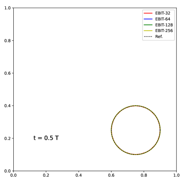
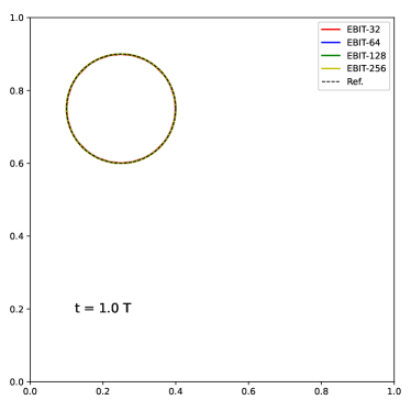
(a)	(b)

Figure 9: Translation test with the new EBIT method at different resolutions: (a) interface lines at halftime; (b) interface lines at the end of the simulation

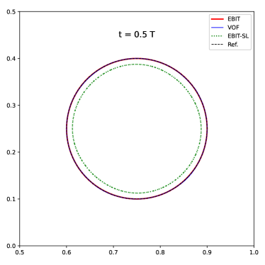
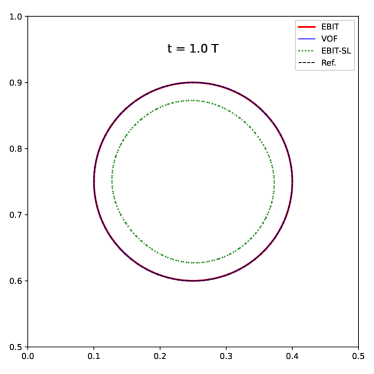
(a)	(b)

Figure 10: Translation test with different methods at resolution $N_{x}=128$: (a) interface lines at halftime; (b) interface lines at the end of the simulation

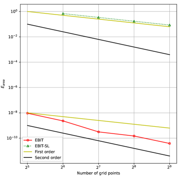
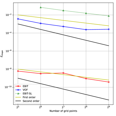
(a)	(b)

Figure 11: Errors in the translation test for different methods as a function of grid resolution: (a) area error $E_{area}$; (b) shape error $E_{shape}$

The interface lines are also calculated with different reconstruction and advection methods for a medium mesh resolution, $N_{x}=128$, and are shown in Fig. 10. Both the new EBIT method and the PLIC-VOF method maintain rather well the circular shape of the interface during the translation. On the other hand, the first version of the EBIT method, that considers a straight line approximation (SL) for the calculation of the position of unaligned markers, loses mass continuously during the simulation.

The area errors $E_{area}$ and the shape errors $E_{shape}$ are listed in Table 1 and are shown in Fig. 11 for the different methods. For the new EBIT method we observe a second-order convergence rate for the area error and approximately a first-order convergence rate for the shape error, as shown in Fig. 11. For the first version of the EBIT method (SL), both the area and shape errors are much larger. Furthermore, this method loses all the reference phase at the lowest grid resolution, $N_{x}=32$ (this fact is denoted by “NA” in Table 1.

Table 1: Mesh convergence study for the translation test

	$N_{x}$	32	64	128	256	512
EBIT	$E_{area}$	$9.32\times 10^{-9}$	$2.30\times 10^{-9}$	$3.13\times 10^{-10}$	$1.48\times 10^{-10}$	$3.82\times 10^{-11}$
	$E_{shape}$	$6.13\times 10^{-9}$	$3.21\times 10^{-9}$	$3.77\times 10^{-9}$	$9.08\times 10^{-10}$	$3.76\times 10^{-10}$
VOF	$E_{shape}$	$3.88\times 10^{-3}$	$1.06\times 10^{-3}$	$4.72\times 10^{-4}$	$2.59\times 10^{-4}$	$2.68\times 10^{-4}$
EBIT-SL	$E_{area}$	NA	$6.83\times 10^{-1}$	$3.41\times 10^{-1}$	$1.70\times 10^{-1}$	$8.52\times 10^{-2}$
	$E_{shape}$	NA	$6.86\times 10^{-2}$	$3.10\times 10^{-2}$	$1.54\times 10^{-2}$	$7.78\times 10^{-3}$

For the PLIC-VOF method, the mass conservation is accurate to machine error and it is not shown in the figure, while the shape error is evaluated with the two endpoints of the PLIC-VOF reconstruction in each cut cell. For this error we observe in Fig. 11a first-order convergence rate. Due to the fact that in the new EBIT method we are fitting a circle with a circle, the shape error obtained with the PLIC-VOF method is larger than that of the new EBIT method.

3.2 Single vortex

The single vortex test was designed to test the ability of an interface tracking method to follow the evolution in time of an interface that is highly stretched and deformed [28]. A circular interface of radius $R=0.15$ and center at $(0.5,0.75)$ is placed inside the unit square domain. A divergence-free velocity field $(u,v)=(\partial\phi\big{/}\partial y,-\partial\phi\big{/}\partial x)$ described by the stream function $\phi=\pi^{-1}\sin^{2}(\pi x)\sin^{2}(\pi y)\cos(\pi t/T)$ is imposed in the domain. The cosinusoidal time-dependence slows down and reverses the flow, so that the maximum deformation occurs at $t=0.5\,T$, where $T$ is the period, then the interface returns to its initial position without distortion at $t=T$. Furthermore, as the value of the period $T$ is increased, a thinner and thinner revolving ligament develops.

In this test we use a constant $CFL$ value, $CFL=0.125$, based on the maximum value of the velocity at time $t=0$. The error is again measured by the area and shape errors. The reference solution is obtained by solving the ordinary differential equations $d\boldsymbol{x}\big{/}dt=\boldsymbol{u}(x(t),y(t),t)$ with a fourth-order Runge-Kutta method.

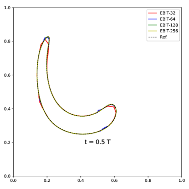
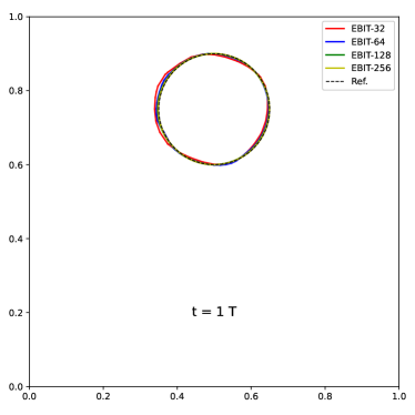
(a)	(b)

Figure 12: Single vortex test with period $T=2$ at different resolutions: (a) interface lines at halftime; (b) interface lines at the end of the simulation

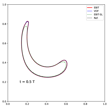
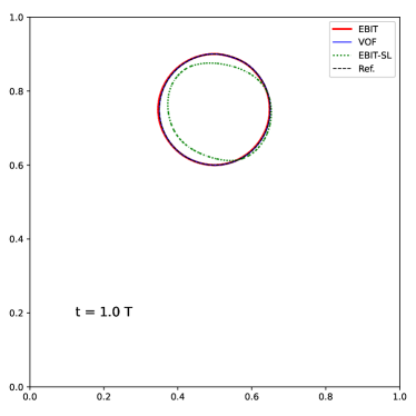
(a)	(b)

Figure 13: Single vortex test with period $T=2$ at resolution $N_{x}=128$ with different methods: (a) interface lines at halftime; (b) interface lines at the end of the simulation

Table 2: Mesh convergence study for the single vortex test with period $T=2$

	$N_{x}$	32	64	128	256	512
EBIT	$E_{area}$	$1.69\times 10^{-2}$	$7.45\times 10^{-3}$	$2.62\times 10^{-3}$	$1.25\times 10^{-3}$	$5.99\times 10^{-4}$
	$E_{shape}$	$1.45\times 10^{-2}$	$6.74\times 10^{-3}$	$3.07\times 10^{-3}$	$1.54\times 10^{-3}$	$7.75\times 10^{-4}$
VOF	$E_{shape}$	$8,79\times 10^{-3}$	$3.00\times 10^{-3}$	$1.17\times 10^{-3}$	$4.11\times 10^{-4}$	$1.21\times 10^{-4}$
EBIT-SL	$E_{area}$	$8.26\times 10^{-1}$	$3.66\times 10^{-1}$	$1.71\times 10^{-1}$	$8.19\times 10^{-2}$	$4.02\times 10^{-2}$
	$E_{shape}$	$1.20\times 10^{-1}$	$5.77\times 10^{-2}$	$2.68\times 10^{-2}$	$1.33\times 10^{-2}$	$6.99\times 10^{-3}$

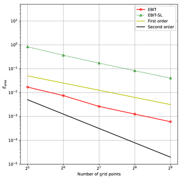
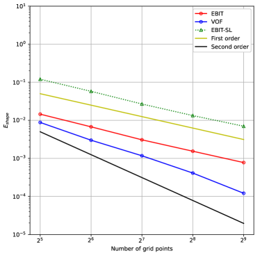
(a)	(b)

Figure 14: Errors in the single vortex test with period $T=2$ for different methods as a function of grid resolution: (a) area error $E_{area}$; (b) shape error $E_{shape}$

The interface line at maximum deformation and back to its initial position, for the test with period $T=2$, is shown in Fig. 12 for different mesh resolutions. Even at the lowest resolution $N_{x}=32$, with the new EBIT method we still recover the initial shape and lose little mass. The interface line obtained with different methods is shown in Fig. 13 for the resolution $N_{x}=128$. The results obtained with the new EBIT method and the PLIC-VOF method agree rather well with each other. For the EBIT method with a straight line fit, we observe a considerable amount of area loss.

The area error $E_{area}$ and the shape error $E_{shape}$ are listed in Table 2 and are shown in Fig. 14 for the different methods here considered. For the new EBIT method that implements a circle fit, a convergence rate between first-order and second-order is observed for both errors. The shape errors calculated with the new EBIT method and with the PLIC-VOF method are of about the same order of magnitude.

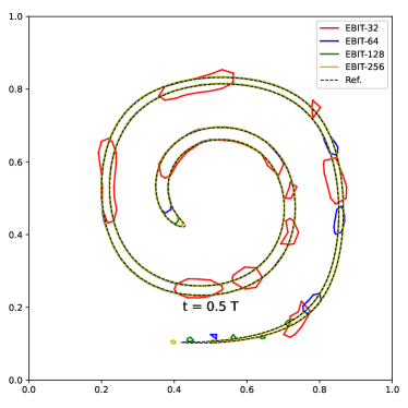
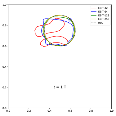
(a)	(b)

Figure 15: Single vortex test with period $T=8$ at different resolutions: (a) interface lines at halftime; (b) interface lines at the end of the simulation

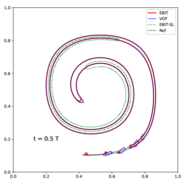
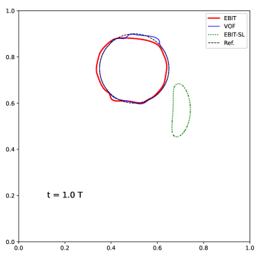
(a)	(b)

Figure 16: Single vortex test with period $T=8$ at resolution $N_{x}=128$ with different methods: (a) interface lines at halftime; (b) interface lines at the end of the simulation

Table 3: Mesh convergence study for the single vortex test with period $T=8$

	$N_{x}$	32	64	128	256	512
EBIT	$E_{area}$	$3.80\times 10^{-1}$	$7.71\times 10^{-2}$	$2.43\times 10^{-2}$	$2.32\times 10^{-3}$	$8.23\times 10^{-5}$
	$E_{shape}$	$1.47\times 10^{-1}$	$4.99\times 10^{-2}$	$2.09\times 10^{-2}$	$7.07\times 10^{-3}$	$3.54\times 10^{-3}$
VOF	$E_{shape}$	$2.57\times 10^{-1}$	$6.58\times 10^{-2}$	$1.35\times 10^{-2}$	$7.67\times 10^{-3}$	$1.34\times 10^{-3}$
EBIT-SL	$E_{area}$	NA	NA	$7.98\times 10^{-1}$	$3.55\times 10^{-1}$	$1.61\times 10^{-1}$
	$E_{shape}$	NA	NA	$2.02\times 10^{-1}$	$1.29\times 10^{-1}$	$8.53\times 10^{-2}$

The interface line at maximum deformation and back to its initial position, for the test with period $T=8$ is shown in Fig. 15 for different mesh resolutions. In this test, the interface line at maximum deformation at halftime is stretched into a long thin ligament. When the mesh resolution is too coarse, i.e. $N_{x}=32$, the new EBIT method loses some mass due to the artificial topological change mechanism. As the mesh resolution is increased, the mass loss progressively decreases and the method recovers better and better the initial circular shape.

The interface line obtained with different methods is shown in Fig. 16 for the resolution $N_{x}=128$. At this intermediate mesh resolution, there is some discrepancy between the final shape obtained with the new EBIT method and that with the PLIC-VOF method. However, they show the same level of deviation from the reference solution.

For the EBIT method with a straight line fit, there is an even more pronounced mass loss. Furthermore, the interface does not return to its initial position due to the lateral shift of the interface with respect to the reference solution, as shown in Fig. 16a at maximum deformation.

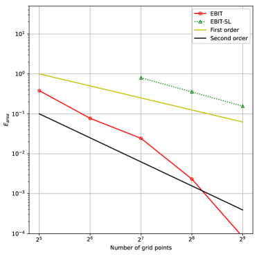
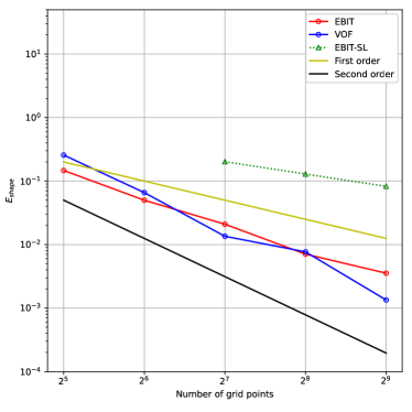
(a)	(b)

Figure 17: Errors in the single vortex test with period $T=8$ for different methods as a function of grid resolution: (a) area error $E_{area}$; (b) shape error $E_{shape}$

The area error $E_{area}$ and the shape error $E_{shape}$ are listed in Table 3 and are shown in Fig. 17. For the new EBIT method, a convergence rate between first-order and second-order is observed for both errors. This behavior is similar to that obtained in the previous test with period $T=2$. The shape errors obtained with the new EBIT method and the PLIC-VOF method become closer to each other as the mesh is refined. The EBIT method with a straight line fit loses all the reference phase even when an intermediate mesh resolution, $N_{x}=64$, is used. All the kinematic tests show that the new EBIT method with a circle fit does decrease the mass loss as the interface is reconstructed, thus increasing the accuracy of mass conservation, and does improve the performance of the EBIT method.

In order to demonstrate the feasibility of the integration of the new EBIT method with AMR, we run again the single-vortex test case on a quadtree grid in Basilisk. The interface lines at halftime and at the end of the simulation and the corresponding meshes are shown in Fig. 18. The maximum level of refinement is $N_{l,max}=7$, which corresponds to the mesh resolution $N_{x}=128$, while the minimum level is $N_{l,min}=4$. All the cells near the interface are refined to the maximum level, to avoid an inconsistency like that shown in Fig. 8. Since the imposed velocity field is not affected by the mesh resolution and the same stencil is used for the velocity interpolation, the interface line obtained on the quadtree grid coincides with that on the fixed Cartesian mesh.

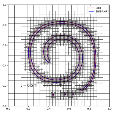
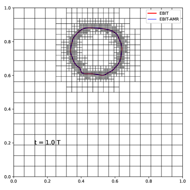
(a)	(b)

Figure 18: Single vortex test with period $T=8$ at fixed resolution $N_{x}=128$ and AMR with $N_{l,max}=7$ and $N_{l,min}=4$: (a) interface lines at halftime; (b) interface lines at the end of the simulation

3.3 Capillary wave

Capillary waves are a basic phenomenon of surface-tension-driven flows and their adequate numerical resolution is a prerequisite to more complex applications. The small-amplitude damped oscillations of a capillary wave are now a classical test case to check the accuracy of new numerical schemes that are developed to investigate the evolution in time of viscous, surface-tension-driven two-phase flows.

A sinusoidal perturbation is applied to a plane interface between two fluids initially at rest. Under the influence of surface tension, the interface begins to oscillate around its equilibrium position, while the amplitude of the oscillations decay in time due to viscous dissipation. The exact analytical solution was found by Prosperetti [29] in the limit of very small amplitudes, and it is usually used as a reference.

In order to get a good agreement with the theory [22], it is necessary to move the top and bottom boundaries far away from the interface, in particular here we consider the rectangular computational domain $[0,\lambda]\times[0,4\lambda]$, where $\lambda$ is the wavelength of the perturbation. A symmetric boundary condition is applied on the four sides of the domain. The initial amplitude of the perturbation is $\lambda/100$, as in Popinet and Zaleski [30], Denner et al. [31] and Gerlach et al. [32]. The value of the other physical properties that are used in the simulation and of the Laplace number, $La=(\rho_{1}\sigma\lambda)\big{/}\mu_{1}^{2}$, is listed in Table 4.

The time evolution of the maximum amplitude of the interface is shown in Fig. 19, together with those of the analytical solution and of the PLIC-VOF method. Time is made dimensionless by using the normal-mode oscillation frequency $\omega_{0}$, which is defined by the dispersion relation

$$\omega_{0}^{2}=\frac{\sigma k^{3}}{2\rho_{1}}$$ (11)

where $k=2\pi/\lambda$ is the wavenumber and with $\lambda=1$ in our simulation. The numerical results obtained with the new EBIT and PLIC-VOF methods agree rather well with the analytical solution.

The error between the theoretical solution [29] and the two numerical solutions can be further analyzed with the $L_{2}$ norm

$$E_{2}=\frac{1}{\lambda}\sqrt{\frac{\omega_{0}}{25}\int_{t=0}^{25/\omega}(h-h_{exact})^{2}}$$ (12)

where $h$ is the maximum interface amplitude obtained with a numerical method and $h_{exact}$ the reference value. The results are shown in Fig. 20 and a convergence rate close to second-order is observed for both methods, the error of the PLIC-VOF method being always somewhat smaller. In both simulations, the height function method has been used to calculate the curvature [22]. More particularly, since we are considering a very small amplitude of the oscillations, thus of the interface curvature as well, the straight line approximation of the new EBIT method in each cut cell provides a fairly good approximation of the volume fraction and hence of the calculation of the local height function.

Table 4: Physical properties for the capillary wave test

$\rho_{1}$	$\rho_{2}$	$\mu_{1}$	$\mu_{2}$	$\sigma$	$La$
$1$	$1$	$0.01826$	$0.01826$	$1$	$3000$

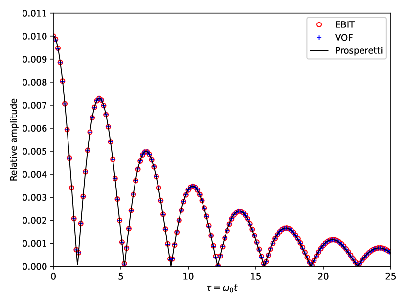
Figure 19: Capillary wave test with different methods: time evolution of the maximum amplitude of the interface oscillation. The time $\tau=\omega_{0}\,t$ is non-dimensional and the grid resolution is $N_{x}\times N_{y}=64\times 256$

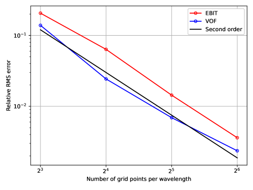
Figure 20: Error $E_{2}$ in the capillary wave test for different methods as a function of grid resolution

3.4 Rayleigh-Taylor instability

In order to demonstrate the capability of the new EBIT method to deal with more complex flows, we investigate another classical test: the Rayleigh-Taylor instability at high Reynolds number, that involves a large deformation of the interface.

The Rayleigh-Taylor instability occurs when a heavy fluid is on top of a lighter one, with the direction of gravity from top to bottom. The density difference between the two fluids plays an important role in the instability and is present in the definition of the dimensionless Atwood number $At$

$$At=\frac{\rho_{1}-\rho_{2}}{\rho_{1}+\rho_{2}}$$ (13)

where $\rho_{1}$ and $\rho_{2}$ are the densities of the heavy and light fluids, respectively.

This instability has been investigated in several studies [33, 34, 35], that consider an incompressible flow without surface tension effects, with $At=0.5$ and different Reynolds numbers, $Re=\big{(}\rho_{1}g^{1/2}d^{3/2}\big{)}\big{/}\mu_{1}$.

In this study, we consider the rectangular computational domain $[0,d]\times[0,4d]$, partitioned with $N_{x}\times N_{y}=128\times 512$ grid cells. The plane interface $y_{0}(x)=2\,d$ between the two fluids is perturbed by a sinusoidal wave $y_{1}(x)=0.1\,d\cos(kx)$, so that the interface line at the beginning of the simulation is

$$y(x)=y_{0}(x)+y_{1}(x)=2\,d+0.1\,d\cos(kx),\quad k=\frac{2\pi}{\lambda}$$ (14)

with $\lambda=d=1$. A no-slip boundary condition is enforced at the bottom and at the top of the computational domain, and a symmetric boundary condition on the two vertical sides. The value of the other physical properties that are used in the simulation and of the Reynolds number $Re$ is listed in Table 5.

Table 5: Physical properties for the Rayleigh-Taylor instability test

$\rho_{1}$	$\rho_{2}$	$\mu_{1}$	$\mu_{2}$	$g$	$Re$
$3$	$1$	$0.00313$	$0.00313$	$9.81$	$3000$

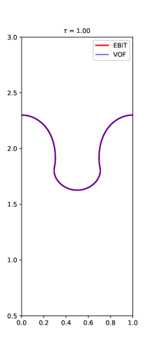
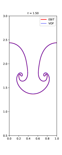
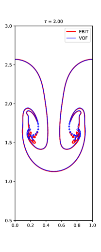
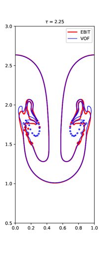
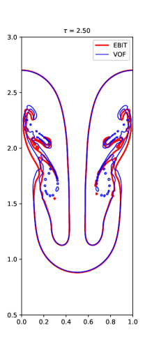
Figure 21: Rayleigh-Taylor instability test with different methods: interface lines at dimensionless times $\tau=1.,1.5,1.75,2.,2.25,2.5$

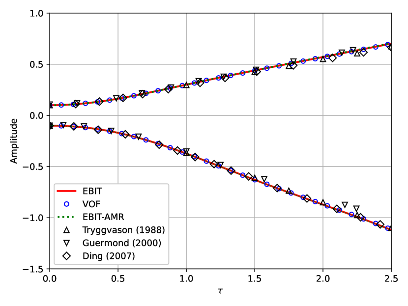
Figure 22: Rayleigh-Taylor instability test with different methods: highest and lowest positions of the interface, with respect to the mean position at $y=2$, as a function of dimensionless time $\tau$

The results of the simulation are first presented in Fig. 21 with the representation of the interface line at several dimensionless times $\tau=t\sqrt{g\,At/d}$. Overall, these results compare rather well with those presented in [35].

More specifically, in the early stages of the simulation, $\tau\leq 1.75$, the shape of interface calculated with the new EBIT method and that with the PLIC-VOF method are in very good agreement, small discrepancies are observed only in the roll-up region where complex structures with thin ligaments start to develop.

Some remarkable differences occur at later times ($\tau\geq 2.00$) when the ligaments start to break up. Due to the mass conservation property of the PLIC-VOF method, many small droplets are formed when the ligaments tear apart. However, in the new EBIT method, these small droplets will soon disappear due to the topology change mechanism. Thus, in the roll-up region, the interface structure obtained with the new EBIT method agrees only qualitatively with that of the PLIC-VOF method.

In spite of this local but consistent difference, very good agreement is observed for the highest and lowest positions of the interface during the whole simulation. The highest position of the rising fluid, near the two vertical boundaries at $x=0,d$, and the lowest position of the falling fluid, near the centerline at $x=d/2$, both computed with respect to the mean position at $y=2\,d$, are shown in Fig. 22. They are in very good agreement with the results obtained with the PLIC-VOF method and those by Tryggvason [33], Guermond [34] and Ding [35].

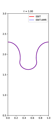
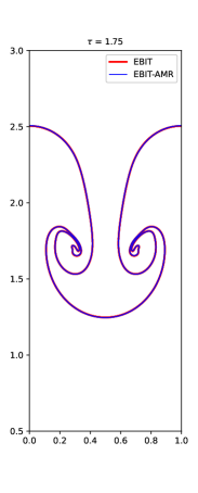
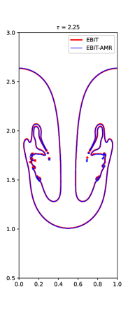
	(a)
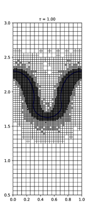
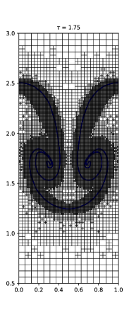
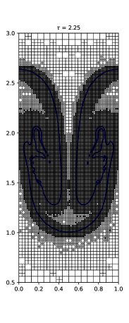
	(b)

Figure 23: Rayleigh-Taylor instability test at dimensionless times $\tau=1.,1.75,2.25$: interface lines with AMR, $N_{l,max}=9$ and $N_{l,min}=6$

Table 6: Computational efficiency of the EBIT method with AMR, Rayleigh-Taylor instability test, $N_{l,max}=9$ and $N_{l,min}=6$

Method	Number of (leaf) cells	Time steps	Wall time (s)
EBIT	$65536$	$5656$	$1741$
EBIT-AMR	$27355$	$5656$	$207$
VOF	$65536$	$5656$	$914$
VOF-AMR	$27223$	$5656$	$151$

The interface lines obtained with the new EBIT method combined with AMR are finally shown in Fig. 23. The maximum level of refinement is now $N_{l,max}=9$, while the minimum level is $N_{l,min}=6$. The refinement criteria are based not only on the position of the interface, but also on the velocity gradient, thus the cells within the roll-up region, characterized by a strong vorticity, are also refined to the maximum level, even if they are not very close to the interface (see Fig. 23b). The interface lines calculated with the new EBIT method on the quadtree grid agree rather well with those on the fixed Cartesian grid (see Fig. 23a), only minor differences are observed in the roll-up region.

The computational efficiency for this test of the new EBIT method with or without AMR is summarized in Table 6. For the PLIC-VOF method with AMR (VOF-AMR), the mesh refinement criteria are based on both curvature and velocity gradient. Without AMR, the dynamics with the new EBIT method is about 2 times slower than with the PLIC-VOF method. But when AMR is used, the wall times for the two methods are comparable.

3.5 Rising bubble

In this test we examine a single bubble rising under buoyancy inside a heavier fluid. This test case was first proposed by Hysing [36] and it provides a standard benchmark for multiphase flow simulations, since this configuration is simple enough to be simulated accurately. Nevertheless, the bubble shows a strong deformation and even complex topology changes in some flow regimes [37, 38], thus giving an adequate challenge to interface tracking techniques.

By taking into account the symmetry with respect to the vertical axis, we consider the rectangular computational domain $[0,D]\times[0,4\,D]$, with $D=0.5$, partitioned with $N_{x}\times N_{y}=128\times 512$ grid cells. At the beginning of the simulation, a circular bubble of radius $R=D/2$ is positioned in the bottom part of the domain with center at $(0,D)$. A no-slip boundary condition is enforced at the bottom and at the top of the computational domain, a free-slip boundary condition on the right vertical wall and a symmetric boundary condition on the left vertical boundary. The value of the relevant physical properties is that provided by Hysing [36] and is listed in Table 7, where $Re=\big{(}\rho_{1}g^{1/2}d^{3/2}\big{)}\big{/}\mu_{1}$ is the Reynolds number and $Bo=\big{(}\rho_{1}gL^{2}\big{)}\big{/}\sigma$ the Bond number.

Table 7: Physical properties for the rising bubble test

Test case	$\rho_{1}$	$\rho_{2}$	$\mu_{1}$	$\mu_{2}$	$g$	$\sigma$	$Re$	$Bo$
$1$	$1000$	$100$	$10$	$1$	$0.98$	$24.5$	$35$	$10$
$2$	$1000$	$1$	$10$	$0.1$	$0.98$	$1.96$	$35$	$125$

We consider the two different test cases of Table 7. In the first test, the bubble should end up in the ellipsoidal regime [36], since the surface tension forces are strong enough to hold the bubble together, hence no breakup is present in the simulation. For this first case, we solve both the axisymmetric problem and the two-dimensional Cartesian one.

The interface lines at the end of the simulation at time $t=3$ are shown in Fig. 24a, for both the axisymmetric and Cartesian problems and with the new EBIT and PLIC-VOF methods. In general, good agreement between the two methods is found in both problems. More particularly, the bubble computed with the PLIC-VOF method is always a very little ahead of the bubble with the new EBIT method.

The rising velocities for the two problems and the two methods as a function of time are shown in Fig. 25a. The figure includes also the results obtained with the new EBIT method in conjunction with AMR. The profiles of the rising velocities are very close to each other and this justify the fact that at the end of the simulation there is very little difference between the interface lines. For the Cartesian problem, the value of the maximum rising velocity is $0.2419$ for the new EBIT method and $0.2418$ for the PLIC-VOF method, which are basically the same value, $0.2419\pm 0.0002$, reported by Hysing [36].

In the second test, the bubble lies somewhere between the skirted and the dimpled ellipsoidal-cap regimes, indicating that breakup can eventually take place. The simulation is carried out with both the new EBIT and PLIC-VOF methods, and the interface lines at the end of the simulation at time $t=3$ are shown in Fig. 24b. At the given mesh resolution, the bubble skirt is observed with both methods, with no interface breakup. Good agreement is observed between the two interface lines. More in detail, the new EBIT method predicts a slightly larger central part of the bubble and a smoother and shorter tail in the skirt region.

The rising velocities for the two methods as a function of time are shown in Fig. 25b. In this case as well, the figure includes the results obtained with the new EBIT method in conjunction with AMR. The presence of two peaks is well predicted in our simulation. The value of the first one is $0.2507$ for the new EBIT method and $0.2512$ for the PLIC-VOF method, in good agreement with the value $0.25\pm 0.01$ indicated by Hysing [36].

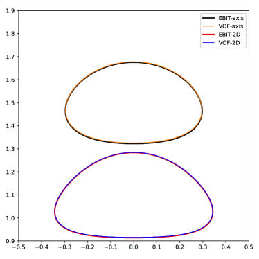
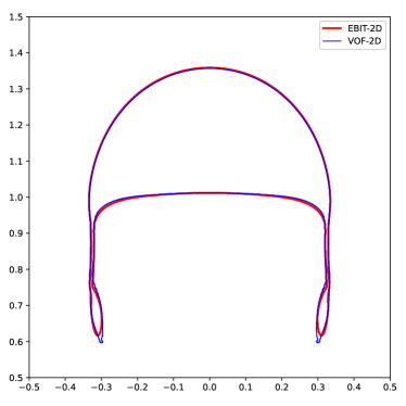
(a)	(b)

Figure 24: Rising bubble test. Interface lines at the end of the simulation $t=3$ with different methods: (a) axisymmetric and Cartesian solutions for test case 1; (b) Cartesian solution for test case 2

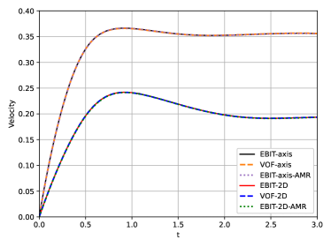
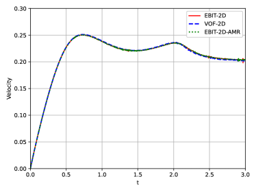
(a)	(b)

Figure 25: Rising bubble test. Bubble velocities as a function of time with different methods: (a) profiles for test case 1, including EBIT with AMR; (b) profiles for test case 2, including EBIT with AMR

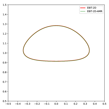
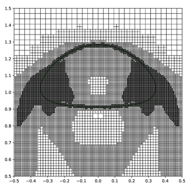
(a)	(b)

Figure 26: Rising bubble test case 1-2D: interface lines at the end of the simulation $t=3$ with AMR, $N_{l,max}=9$ and $N_{l,min}=6$

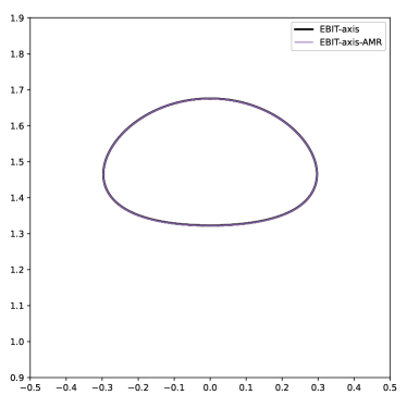
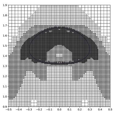
(a)	(b)

Figure 27: Rising bubble test case 1-Axisymmetric: interface lines at the end of the simulation $t=3$ with AMR, $N_{l,max}=9$ and $N_{l,min}=6$

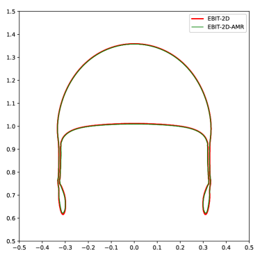
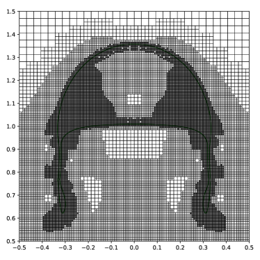
(a)	(b)

Figure 28: Rising bubble test case 2-2D: interface lines at the end of the simulation $t=3$ with AMR, $N_{l,max}=9$ and $N_{l,min}=6$

Table 8: Computational efficiency of the EBIT method with AMR, rising bubble test, $N_{l,max}=9$ and $N_{l,min}=6$

	Method	Number of (leaf) cells	Time steps	Wall time (s)
Case1-2D	EBIT	$65536$	$4606$	$1726$
	EBIT-AMR	$11077$	$4606$	$172$
	VOF	$65536$	$4607$	$935$
	VOF-AMR	$10852$	$4607$	$147$
Case1-Axi	EBIT	$65536$	$4606$	$1824$
	EBIT-AMR	$10141$	$4606$	$166$
	VOF	$65536$	$4607$	$1136$
	VOF-AMR	$9937$	$4607$	$145$
Case2-2D	EBIT	$65536$	$1599$	$4653$
	EBIT-AMR	$14392$	$1595$	$729$
	VOF	$65536$	$1536$	$3577$
	VOF-AMR	$14053$	$1535$	$751$

When AMR is considered, the refinement criteria are those that have been used in the Rayleigh-Taylor instability test, i.e. proximity to the interface and velocity gradient. The maximum level of refinement is $N_{l,max}=9$, while the minimum level is $N_{l,min}=6$, for both test cases. The interface lines at the end of the simulation at time $t=3$ are shown in Figs. 26 and 27 for test case 1, and in Figs. 28 for test case 2.

For the axisymmetric problem, the interface line calculated by the new EBIT method on the quadtree grid is on top of the line on the fixed Cartesian grid. For the two Cartesian problems, the interface line on the quadtree grid is just a little bit behind that on the fixed Cartesian grid.

The computational efficiency for these two cases of the new EBIT method with or without AMR is summarized in Table 8. Without AMR, the dynamics with the new EBIT method is about 2 times slower than with the PLIC-VOF method, for test case 1 and the Cartesian problem. For test case 2, with a much smaller surface tension coefficient, the two wall times are closer to each other. The axisymmetric problem is somewhat intermediate. When AMR is used, the wall times of the two methods are comparable, in agreement with the results obtained in the Rayleigh-Taylor instability test.

4 Conclusions

We present a novel Front-Tracking method, the Edge-Based Interface Tracking (EBIT) method, which is more suitable for parallelization due to the lack of explicit connectivity. Several new features have been introduced to improve the very first version of the EBIT method [20]. First, a circle fit has been implemented to improve the accuracy of mass conservation after the interface advection in the reconstruction phase. Second, a Color Vertex feature has been introduced to distinguish between ambiguous topological configurations and to represent the connectivity implicitly. Third, an automatic topological change mechanism has been discussed.

The new EBIT method has been implemented inside the open-source Basilisk platform in order to solve the Navier–Stokes equations for multiphase flow simulations with surface tension. Volume fractions are calculated based on the position of the markers and the Color Vertex, and are used to calculated the physical properties and the surface tension force. To improve the computational efficiency and to avoid inconsistencies, AMR can be used with the EBIT method by considering a careful refinement strategy.

Numerical results for various cases, including both kinematic and dynamical tests, have been considered and compared with those obtained with the VOF method. Good agreement is observed for all test cases.

In future work, we aim to remove the restriction on the number of markers on a cell side, to improve our control on topological changes, and to extend the EBIT method to three dimensions.

5 CRediT authorship contribution statement

J. Pan: Conceptualization, Formal analysis, Code development, Simulations, Writing

T. Long: Formal analysis, Code development

L. Chirco: Conceptualization, Code development

R. Scardovelli: Formal analysis, Writing

S. Popinet: Basilisk code development

S. Zaleski: Conceptualization, Formal analysis, Supervision, Writing, Funding acquisition

6 Declaration of competing interest

The authors declare that they have no known competing financial interests or personal relationships that could have appeared to influence the work reported in this paper.

7 Acknowledgements

Stéphane Zaleski and Stéphane Popinet recall meeting Sergei Semushin in March 1995 and learning about his method. They thank him for the explanation of the method. This project has received funding from the European Research Council (ERC) under the European Union’s Horizon 2020 research and innovation programme (grant agreement number 883849).

References

- Or [2018] D. Or, The tyranny of small scales–on representing soil processes in global land surface models, Water Resources Research (2018).
- Hirt and Nichols [1981] C. Hirt, B. Nichols, Volume of fluid (VOF) method for the dynamics of free boundaries, Journal of Computational Physics 39 (1981) 201–225.
- Brackbill et al. [1992] J. Brackbill, D. Kothe, C. Zemach, A continuum method for modeling surface tension, Journal of Computational Physics 100 (1992) 335–354.
- Osher and Sethian [1988] S. Osher, J. A. Sethian, Fronts propagating with curvature-dependent speed: Algorithms based on Hamilton-Jacobi formulations, Journal of Computational Physics 79 (1988) 12–49.
- Osher and Fedkiw [2001] S. Osher, R. P. Fedkiw, Level set methods: An overview and some recent results, Journal of Computational Physics 169 (2001) 463–502.
- Unverdi and Tryggvason [1992] S. O. Unverdi, G. Tryggvason, A front-tracking method for viscous, incompressible, multi-fluid flows, Journal of Computational Physics 100 (1992) 25–37.
- Tryggvason et al. [2011] G. Tryggvason, R. Scardovelli, S. Zaleski, Direct Numerical simulations of gas-liquid multiphase flows, Cambridge University Press, 2011.
- Chen et al. [1997] S. Chen, D. B. Johnson, P. E. Raad, D. Fadda, The surface marker and micro cell method, International Journal for Numerical Methods in Fluids 25 (1997) 749–778.
- Chen et al. [2022] X. Chen, J. Lu, S. Zaleski, G. Tryggvason, Characterizing interface topology in multiphase flows using skeletons, Physics of Fluids 34 (2022) 093312.
- Chirco et al. [2022] L. Chirco, J. Maarek, S. Popinet, S. Zaleski, Manifold death: A volume of fluid implementation of controlled topological changes in thin sheets by the signature method, Journal of Computational Physics 467 (2022) 111468.
- Chiodi [2020] R. M. Chiodi, Advancement of Numerical Methods for Simulating Primary Atomization, Ph.D. thesis, Cornell University, 2020.
- Aulisa et al. [2003] E. Aulisa, S. Manservisi, R. Scardovelli, A mixed markers and volume-of-fluid method for the reconstruction and advection of interfaces in two-phase and free-boundary flows, Journal of Computational Physics 188 (2003) 611–639.
- Aulisa et al. [2004] E. Aulisa, S. Manservisi, R. Scardovelli, A surface marker algorithm coupled to an area-preserving marker redistribution method for three-dimensional interface tracking, Journal of Computational Physics 197 (2004) 555–584.
- López et al. [2005] J. López, J. Hernández, P. Gómez, F. Faura, An improved PLIC-VOF method for tracking thin fluid structures in incompressible two-phase flows, Journal of Computational Physics 208 (2005) 51–74.
- Shin and Juric [2002] S. Shin, D. Juric, Modeling three-dimensional multiphase flow using a level contour reconstruction method for front tracking without connectivity, Journal of Computational Physics 180 (2002) 427–470.
- Shin et al. [2005] S. Shin, S. Abdel-Khalik, V. Daru, D. Juric, Accurate representation of surface tension using the level contour reconstruction method, Journal of Computational Physics 203 (2005) 493–516.
- Shin and Juric [2007] S. Shin, D. Juric, High order level contour reconstruction method, Journal of Mechanical Science and Technology 21 (2007) 311–326.
- Singh and Shyy [2007] R. Singh, W. Shyy, Three-dimensional adaptive cartesian grid method with conservative interface restructuring and reconstruction, Journal of Computational Physics 224 (2007) 150–167.
- Shin et al. [2011] S. Shin, I. Yoon, D. Juric, The local front reconstruction method for direct simulation of two- and three-dimensional multiphase flows, Journal of Computational Physics 230 (2011) 6605–6646.
- Chirco and Zaleski [2022] L. Chirco, S. Zaleski, An edge-based interface-tracking method for multiphase flows, International Journal for Numerical Methods in Fluids 95 (2022) 491–497.
- Popinet [2003] S. Popinet, Gerris: a tree-based adaptive solver for the incompressible euler equations in complex geometries, Journal of Computational Physics 190 (2003) 572–600.
- Popinet [2009] S. Popinet, An accurate adaptive solver for surface-tension-driven interfacial flows, Journal of Computational Physics 228 (2009) 5838–5866.
- Yoon and Shin [2010] I. Yoon, S. Shin, Tetra-marching procedure for high order level contour reconstruction method, WIT Transactions on Engineering Sciences (2010).
- Scardovelli and Zaleski [2000] R. Scardovelli, S. Zaleski, Analytical relations connecting linear interfaces and volume fractions in rectangular grids, J. Comput. Phys. 164 (2000) 228–237.
- Bell et al. [1989] J. B. Bell, P. Colella, H. M. Glaz, A second-order projection method for the incompressible Navier-Stokes equations, Journal of Computational Physics 85 (1989) 257–283.
- Popinet [2018] S. Popinet, Numerical models of surface tension, Annual Review of Fluid Mechanics 50 (2018) 49–75.
- Popinet [2015] S. Popinet, A quadtree-adaptive multigrid solver for the Serre–Green–Naghdi equations, Journal of Computational Physics 302 (2015) 336–358.
- Rider and Kothe [1998] W. J. Rider, D. B. Kothe, Reconstructing volume tracking, Journal of Computational Physics 141 (1998) 112–152.
- Prosperetti [1981] A. Prosperetti, Motion of two superposed viscous fluids, Physics of Fluids 24 (1981) 1217.
- Popinet and Zaleski [1999] S. Popinet, S. Zaleski, A front-tracking algorithm for accurate representation of surface tension, International Journal for Numerical Methods in Fluids 30 (1999) 775–793.
- Denner et al. [2017] F. Denner, G. Paré, S. Zaleski, Dispersion and viscous attenuation of capillary waves with finite amplitude, The European Physical Journal Special Topics 226 (2017) 1229–1238.
- Gerlach et al. [2006] D. Gerlach, G. Tomar, G. Biswas, F. Durst, Comparison of volume-of-fluid methods for surface tension-dominant two-phase flows, International Journal of Heat and Mass Transfer 49 (2006) 740–754.
- Tryggvason [1988] G. Tryggvason, Numerical simulations of the Rayleigh-Taylor instability, Journal of Computational Physics 75 (1988) 253–282.
- Guermond and Quartapelle [2000] J.-L. Guermond, L. Quartapelle, A projection FEM for variable density incompressible flows, Journal of Computational Physics 165 (2000) 167–188.
- Ding et al. [2007] H. Ding, P. D. Spelt, C. Shu, Diffuse interface model for incompressible two-phase flows with large density ratios, Journal of Computational Physics 226 (2007) 2078–2095.
- Hysing et al. [2009] S. Hysing, S. Turek, D. Kuzmin, N. Parolini, E. Burman, S. Ganesan, L. Tobiska, Quantitative benchmark computations of two-dimensional bubble dynamics, International Journal for Numerical Methods in Fluids 60 (2009) 1259–1288.
- Clift et al. [1978] R. Clift, J. Grace, M. E. Weber, Bubbles, drops, and particles, Academic Press, New York, 1978.
- Legendre [2022] D. Legendre, Free rising skirt bubbles, Physical Review Fluids 7 (2022) 093601.