Causal Inference under Network Interference Using a Mixture of Randomized Experiments
Abstract
In randomized experiments, the classic stable unit treatment value assumption (SUTVA) states that the outcome for one experimental unit does not depend on the treatment assigned to other units. However, the SUTVA assumption is often violated in applications such as online marketplaces and social networks where units interfere with each other. We consider the estimation of the average treatment effect in a network interference model using a mixed randomization design that combines two commonly used experimental methods: Bernoulli randomized design, where treatment is independently assigned for each individual unit, and cluster-based design, where treatment is assigned at an aggregate level. Essentially, a mixed randomization experiment runs these two designs simultaneously, allowing it to better measure the effect of network interference. We propose an unbiased estimator for the average treatment effect under the mixed design and show the variance of the estimator is bounded by where is the maximum degree of the network, is the network size, and is the probability of treatment. We also establish a lower bound of for the variance of any mixed design. For a family of sparse networks characterized by a growth constant , we improve the upper bound to . Furthermore, when interference weights on the edges of the network are unknown, we propose a weight-invariant design that achieves a variance bound of .
Keywords experimental design causal inference network interference clustering SUTVA
1 Introduction
Randomized experiments are a powerful tool for understanding the causal impact of changes. For example, online marketplaces use randomized experiments to test the effectiveness of new features (Johari et al.,, 2022); tech companies build large-scale experimentation platforms to improve their products and systems (Paluck et al.,, 2016; Saveski et al.,, 2017); economists and social science researchers rely heavily on randomized experiments to understand the effects of economic and social changes (Leung, 2022a, ). The overarching goal of randomized experiments is to impute the difference between two universes that cannot be observed simultaneously: a factual universe where the treatments assigned to all units remain unchanged, and a counterfactual universe where all units receive a new treatment. The difference in the average outcome between these two universes is commonly known as the average treatment effect (ATE). Standard estimation approaches for the ATE such as A/B testing rely heavily on a fundamental independence assumption: the stable unit treatment value assumption (SUTVA) (Imbens and Rubin,, 2015), which states that the outcome for each experimental unit depends only on the treatment it received, and not on the treatment assigned of any other units.
However, SUTVA is often violated in settings where experimental units interact with each other. In such cases, ignoring the interference between treatment and control groups may lead to significant estimation bias of the ATE. For example, suppose an e-commerce retailer wants to determine the causal effect on its sales by applying a price promotion to all products. One simple approach is to run an experiment that applies promotion randomly to a subset of products, and then compare the average sales of promoted products with non-promoted products. However, simply comparing the difference in the two groups will likely overestimate the average treatment effect of the promotion, because customers may alter their shopping behavior in the experiment by substituting non-promoted products for similar promoted products. As such, if the retailer decides to implement the price promotion for all products on its platform based on the result of this experiment, the realized sales lift may be smaller than expected.
One common approach for reducing the estimation bias of ATE in the presence of interference is cluster-based randomization, which assigns treatment at an aggregate level rather than at the individual level. In such a design, the population of the experiment is often represented by an underlying network , where each vertex in the set represents an individual experimental unit, and a directed edge indicates that the outcome of unit may be affected by the treatment of another unit . The weights on the edges represent the magnitude of interference between two units. Note that the weights on and can be different, as the interference between two units may be asymmetric. A cluster-based randomization design partitions the network into disjoint subsets of vertices (i.e., clusters) and applies the same treatment to all units within the same cluster. Clearly, using larger clusters will reduce the number of edges across clusters and will better capture the network interference effect between units, which leads to a smaller bias. However, a downside of using larger clusters is that there will be fewer randomization units in the experiment, resulting in higher variance in the ATE estimation. Considering this bias-variance trade-off, a substantial body of literature delves into optimal cluster design under network interference (Ugander et al.,, 2013; Candogan et al.,, 2023; Leung, 2022b, ; Brennan et al.,, 2022).
In this paper, we propose a modification of cluster-based randomization by mixing it with another commonly used experiment design in which each unit is individually and independently randomized, i.e., Bernoulli randomization. As one experimental unit cannot receive two different treatments at the same time, the mixed design determines which randomization method applies to a given unit by a coin flip. Essentially, the mixed design simultaneously runs a cluster-based randomized experiment on one half of the network and an individually randomized experiment on the other half. The idea of mixing cluster-based and Bernoulli designs is proposed by (Saveski et al.,, 2017; Pouget-Abadie et al., 2019b, ), which uses the mixed design to detect the existence of network inference effect (i.e., hypothesis testing for SUTVA). But to the best of our knowledge, the effect of using mixed randomization design in estimating average treatment effects has not been previously studied.
We summarize the main results of the paper as follows. In Section 3, we define an unbiased estimator for the ATE under mixed randomization designs and establish bounds on the variance of the estimator given any cluster design (which is used in the cluster-based part of the experiment). Due to computational challenges, these variance bounds cannot be directly applied to optimize cluster design. We propose several heuristics for clustering and analyze the variance of the estimator in these heuristics. For general networks, we prove a bound on the ATE estimation variance in the order of where is the maximum degree of the network, is the network size, and is the fraction of units that receive treatment. Our result improves the state-of-the-art upper bound in Ugander and Yin, (2023), which uses cluster-based randomization design. We also establish a lower bound of for any mixed design that matches the upper bound up to a factor of . For a family of sparse networks characterized by a growth constant , we improve the upper bound to .
In Section 4, we extend the analysis to the case where the degree of interference between units, namely, the edge weights of the network, are unknown a priori. We propose a weight-invariant mixed randomization design that is agnostic to edge weights, and show the algorithm has an upper bound on the estimation variance in the order of . Furthermore, we show that our proposed estimators are consistent and asymptotically normal provided that the graph is sufficiently sparse (Section 5). Finally, we use numerical experiments to illustrate the efficacy of the proposed mixed randomization algorithms in Section 6 and compare it with (pure) cluster-based randomization.
2 Related Works
There is extensive literature that explores experiment design where experimental units interfere with each other. Halloran and Struchiner, (1995) considered designing and analyzing experiments with interference motivated by infectious diseases. Hudgens and Halloran, (2008) extended their work by estimating the causal effects of treatments when interference exists within disjoint groups. Manski, (2013) and Aronow and Samii, (2017) further generalized the approach to problems where interference is represented by a treatment vector known as exposure mapping. The exposure mapping framework forms a foundation for subsequent studies of various types of experiments, such as graph experiment (Ugander et al.,, 2013; Ugander and Yin,, 2023), bipartite experiment (Pouget-Abadie et al., 2019a, ; Brennan et al.,, 2022; Harshaw et al.,, 2023), switchback experiment (Bojinov et al.,, 2023), and micro-randomized trials (Li and Wager,, 2022), among others.
When the SUTVA assumption is violated by interference between units, several experiment design approaches have been proposed to to mitigate the estimation bias. One common approach is cluster-based randomization, which partitions units into clusters and then assigns random treatments at the cluster level. Previous studies have shown that cluster-based design can reduce bias when interference exists (Eckles et al.,, 2016; Leung, 2022b, ) as well as estimation variance under neighborhood interference (using an unbiased Horvitz-Thompson (HT) estimator) (Ugander et al.,, 2013; Ugander and Yin,, 2023). Another approach is using a multi-level randomization design where treatments are applied with different proportions to groups, assuming that there is no interference between groups (Hudgens and Halloran,, 2008; Tchetgen and VanderWeele,, 2012). A third approach is using regression adjustment in experiments with covariates to improve estimation precision (Chin,, 2019).
Our work studies causal inference with network interference. Specifically, we consider a setting with linear exposure mapping, which is a generalization of the partial interference assumption and stratified interference assumption in Hudgens and Halloran, (2008). The linear exposure mapping assumption is also common in studies of bipartite experiments (Brennan et al.,, 2022; Harshaw et al.,, 2023)) and social network experiments (Bramoullé et al.,, 2009; Toulis and Kao,, 2013; Pouget-Abadie et al., 2019b, ). Another common assumption on the exposure mapping in the literature is that interference solely comes from a unit’s neighbors (Ugander et al.,, 2013; Ugander and Yin,, 2023) and otherwise allows for inference under arbitrary exposure mappings. More recently, problems under more general exposure mapping assumptions have been studied. For example, Leung, 2022b studied the case where interference may be present between any pair of units but the extent of interference diminishes with spatial distance. A similar analysis was also presented in Leung, 2022a . Sävje, (2023) considered the setting where the exposure mapping may be misspecified and discussed the conditions under which unbiased causal effects can be estimated.
Our main goal in this paper is to correctly estimate the average treatment effect (ATE) under network inference. In addition to this goal, there are other goals that have attracted the attention of researchers. Saveski et al., (2017) and Pouget-Abadie et al., 2019b considered a hypothesis testing problem of detecting the existence of network interference. Our approach is partially motivated by the randomization over randomized experiments approach proposed in those papers. Sävje et al., (2021) considered the inferential target of estimating the direct treatment effect under unknown interference. Candogan et al., (2023) developed a family of experiments called independent block randomization, which aims at correlating the treatment probability of clusters to minimize the worse-case variance.
3 Analysis of Mixed Randomization Design
3.1 Notation
Let for any . And let be the set of integers for any and . Throughout the paper, we use the boldface symbols (e.g., ) to denote a vector and to denote its element.
3.2 Network Causal Inference Model
Below, we define a causal inference problem with network interference using the exposure mapping framework (Aronow and Samii,, 2017). Consider an experiment with individual units. Each unit is associated with a potential outcome function , which maps a treatment vector to a potential outcome value. Let the average expected outcome of all units given the assignment be
Let be a vector of 1’s and be a vector of 0’s. Our goal is to measure the (global) average treatment effect (ATE): .
Because the number of possible treatment assignments is exponential in (i.e., ), making causal inferences on the ATE is impractical unless further assumption is imposed on the structure of the outcome function . Throughout this paper, we assume that depends only on the treatments of units from a subset , which is referred to as the neighborhood set of unit . More formally, for any two assignment vector and such that and for all , we have . We assume that the neighborhood set is known and correctly specified for each unit. By connecting units with their neighbors, we get a directed graph where is the set of all units and is the set of all edges. Without loss of generality, we assume the graph is connected; otherwise, the problem can be decomposed into separate subgraphs.
We focus on a linear exposure model where the magnitude of interference on unit from unit is measured by a constant factor , . Without loss of generality, we assume the weights are normalized such that and . The outcome function of unit is given by
| (1) |
In Eq (1), is the potential outcome of unit without any treatment, is the direct treatment effect on unit , is the spillover effect from an adjacent unit . Because , the value can be interpreted as the maximum absolute interference effect from neighbors. We treat the coefficients , , and as fixed but unknown so that the only randomness in the observation model is due to the choice of treatment assignment . In this section, we assume the weights ’s are known. For example, Saveski et al., (2017) considers a social network experiment where each unit represents a user and is the same for all (up to a normalization factor). As another example, for an experiment on a transportation network, we may set as the traffic flow from node to node . The setting with unknown ’s will be studied in Section 4.
The linear exposure mapping model in Eq (1) can be viewed as a first-order approximation of more general network interference patterns. Similar linear exposure assumptions are common in the causal inference literature (Toulis and Kao,, 2013; Brennan et al.,, 2022; Harshaw et al.,, 2023) and our model generalizes some previous studies by allowing weighted inference from neighboring units. Throughout the paper, we assume the outcomes are bounded, that is, there exist constants and such that for all and all . We also assume without loss of generality (e.g., by shifting the outcome of all units by a fixed constant).
One common approach used in the literature to reduce the bias of ATE under network interference is cluster-based randomization, where the network is partitioned into disjoint clusters, and units within the same cluster are assigned the same treatment. Specifically, let and let the clusters be a partition of the vertex set . We define as a function that maps the index of unit to its associated cluster, i.e., if and only if . The standard estimator for ATE in cluster-based design is the Horvitz-Thompson estimator, which is defined below.
Definition 1 (Cluster-based Randomization).
Let be the treatment probability. Under cluster-based randomized design, each unit’s treatment is a Bernoulli random variable, i.e. Bernoulli() for all . Moreover, for , the correlation coefficient of and is corr. The Horvitz-Thompson (HT) estimator for the ATE in cluster-based design (denoted by the subscript cb) is
| (2) |
We note that there exist other definitions of HT estimators in cluster-based randomization design (e.g. Ugander et al.,, 2013) to make it unbiased, but the HT estimator defined in Eq (2) is commonly used one in practice.
It is easily verified that for the linear exposure mapping model given by Eq (1), the true ATE is equal to , where . However, the expectation of the HT estimator is not always equal to the ATE.
Lemma 1.
Let be the HT estimator of cluster-based design in Definition 1. Its expectation is given by
| (3) |
Proof.
By Lemma 1, the HT estimator of a cluster-based design is unbiased if and only if all clusters are independent, i.e., there does not exist such that but . Nevertheless, in most randomized experiments, the underlying network cannot be perfectly partitioned into independent clusters.
As a motivating example, let us consider a -regular network (i.e. for every ) with for all . The ATE for this network is . However, assuming between-cluster connections account for half of all the connections, the HT estimator gives , which may cause significant bias in the ATE estimation. To reduce the bias, we may additionally use a Bernoulli randomization design, where each individual unit receives an i.i.d. treatment with probability . The Bernoulli design can be viewed as a special case of cluster-based design where each cluster contains a single unit, i.e. and . By Lemma 1, the mean of the HT estimator for the Bernoulli design is . If we were able to get estimations from both and , we can use a new estimator , which is an unbiased estimator for the ATE with . However, this estimation approach is infeasible, as each unit in the network can only receive one treatment at a time, so we cannot obtain both and .
The challenge above motivates us to consider a mixture of two randomization designs, which we call the mixed design. In the mixed design, we first draw random numbers to determine whether a unit will receive treatment according to a cluster-based design or a Bernoulli design, and then assign treatments according to each design separately. The key idea of the mixed design is to simultaneously obtain estimations from both the cluster-based and Bernoulli designs. The formal definition of the mixed design will be presented in the next subsection.
Finally, we provide lower and upper bounds of the HT estimator for the cluster-based design, which will be used in subsequent sections. The proof is given in Appendix A.
Proposition 2.
The variance of the HT estimator under cluster-based design is bounded by
| (4) |
where
3.3 Mixed Randomization Design
Our proposed mixed design assigns treatment using a two-stage randomization. In the first stage, all nodes in the network are randomly partitioned into two subsets. In the second stage, one subset receives random treatments according to a cluster-based design, and the other subset receives random treatments according to a Bernoulli design. (Random numbers used in the two stages are independent.) We note that similar mixed designs are proposed by Saveski et al., (2017); Pouget-Abadie et al., 2019b . However, their papers focus on hypothesis testing for the existence of network inference, whereas our work aims to estimate the ATE.
The complete steps of creating a mixed randomization design are described as follows:
-
1.
Let be a set of clusters that forms a partition of the network . Let be a random vector indicating the assignment of each cluster to either cluster-based or Bernoulli design. That is, implies that the cluster uses cluster-based design, and implies the cluster uses Bernoulli design. We require to be i.i.d. Bernoulli random variables with mean (). Let be the corresponding unit-level assignment vector, namely, for all .
-
2.
For cluster (): if , assign all the units in this cluster treatment with probability , and assign all the units treatment with probability . If , assign treatment to the units in cluster by i.i.d. Bernoulli variables with mean .
Note that the above procedure does not specify how the clusters should be chosen. We will study how to design clustering algorithms to optimize the efficiency of the mixed randomization design in the next subsection.
Define the following estimators for those units using cluster-based design and for those units using Bernoulli design:
| (5a) | ||||
| (5b) | ||||
It is easily verified that and (the proof is similar to Lemma 1 and is thus omitted). Using this fact, we define the estimator for the mixed randomization design.
Definition 2 (ATE Estimator in Mixed Design).
The following lemma shows that is indeed an unbiased estimator for the ATE.
Lemma 3.
If is given by Eq (6), we have
Proof.
The equality follows immediately from Definition 2. ∎
Note that computing the coefficient by Eq (6) requires full knowledge of the weight coefficients on all edges . Analogous to Proposition 2, we have the following lower and upper bounds on the variance of .
Proposition 4.
Suppose there exist and such that for all and all . Then, we have
| (7) | ||||
| (8) |
where
The proof of Proposition 4 can be found in Appendix A. Note that the variance bounds in Proposition 4 for the estimator under mixed design have a similar form as the variance bound under cluster-based design (see Prop. 2). In particular, the bounds depend on the number and sizes of the clusters (), and the weights of between-cluster connections (). Proposition 4 also provides a bound on the maximum size of each cluster if is consistent. When for all , we have . If as the population size goes to infinity, we must have by the first term of the bound, which implies . Using Proposition 4, we propose an efficient clustering algorithm to upper bound the variance of in Section 3.4. We then provide a lower bound on the variance of for any clustering algorithm in Section 3.5.
3.4 Upper Bound on the Estimator Variance
Recall that Eq (7) in Proposition 4 provides an expression for an upper bound of the variance of the mixed design estimator . However, finding an exact algorithm to minimize the expression in Eq (7) is computationally challenging, as it requires us to optimize the factor in the first term. Andreev and Räcke, (2004) showed that no polynomial time approximation algorithm can guarantee a finite approximation ratio in graph partitioning (in our case, a finite bound on ) unless . Therefore, instead of searching for an optimal algorithm to minimize the bound in Eq (7), we resort to finding an efficient clustering algorithm that leads to an asymptotic bound on .
We first consider arbitrary network structures and propose a clustering algorithm based on a greedy heuristic (Algorithm 1). The key idea is to use maximum weight matching to generate clusters with sizes of 1 and 2, and then merge these small clusters together to create the desired clustering. The merging step follows a greedy rule, where we iteratively look for two clusters to merge to minimize an approximation of the variance upper bound:
| (9) |
where , , and are defined in Proposition 4 and . The main differences between the approximate variance upper bound and the variance upper bound in Proposition 4 are: (1) we replace the unknown parameter by a known value and take the absolute value of ; (2) the term is omitted. After merging two clusters , we obtain a new cluster set , and the corresponding approximate variance upper bound becomes . We use to denote the value of :
| (10) |
Within each iteration, the algorithm looks for a pair of clusters minimizing the value of . The stopping criterion is to check whether is positive, which tells whether the approximate variance upper bound can be further improved by merging clusters.
Note that the computational complexity of Algorithm 1 is . Firstly, finding a maximum matching in a general graph with vertices is (Galil, 1986), thus line 1 to 4 in Algorithm 1 takes time. Secondly, the while loop from Line 5 to Line 7 can iterate at most times since there are vertices. Finally, Line 6 can be implemented in time if we enumerate the edge set to find all adjacent clusters and calculate for every adjacent . Thus, Line 5 to Line 7 in Algorithm 1 takes time, in which is the edge set and thus .
Throughout the paper, we use to denote the maximum degree of the network. The variance of using the output of Algorithm 1 is bounded as follows.
Theorem 5.
The variance of the estimator in mixed randomization design using clustering from Algorithm 1 is upper bounded by .
The complete proof is included in Appendix A. Theorem 5 guarantees an upper bound on the variance of for general networks. For networks with , the estimator is consistent, as the variance converges to 0 as the network size .
The dependence on can be further improved by making additional assumptions on the sparsity of the network. Specifically, we consider a family of graphs satisfying the restricted-growth condition (Ugander et al.,, 2013).
Definition 3 (restricted-growth graph).
Let be the set of vertices within hops of a vertex (i.e., all vertices connected to by a path with length no more than ). A graph is a restricted-growth graph if there exists a constant , such that for all vertices and all , it holds that .
By definition, we have . Empirical evidence shows that the growth constant for most networks in practice can be significantly less than . For example, the empirical analysis by Ugander and Yin, (2023) on Facebook social networks shows that is typically on the order of of .
Assuming the restricted-growth condition, when the spillover effects from neighbors are either always positive or always negative, we propose another clustering algorithm (Algorithm 2). The algorithm has two steps. In the first step, it finds a vertex whose 2-hop does not overlap with any existing cluster, and adds the 2-hop of as a new cluster. Note that by Definition 3, the size of each 2-hop is no more than . In the second step, it forms clusters among the remaining vertices to ensure that the maximum cluster size does not exceed . We show that Algorithm 2 gives a tighter upper bound on the estimation variance , which is linear in the maximum degree of the network.
Theorem 6.
If for all and there exists a positive constant such that for all , the variance of estimator using clustering from Algorithm 2 is upper bounded by .
The bounds in Theorem 5 and 6 compare favorably to the state-of-the-art variance bounds for ATE estimators under cluster-based randomization design. Ugander and Yin, (2023) achieved an variance bound for restricted-growth graphs, which implies an bound for general graphs (since ). Our bounds for mixed randomization design have better dependence on the maximum degree for both general networks and restricted-growth graphs.
3.5 Lower Bound on the Estimator Variance
To put the upper bounds in Section 3.4 into perspective, we present a lower bound of the variance of for any clustering algorithm. To establish the lower bound, we consider a specific family of networks and measure the dependence on the maximum degree and the growth constant by applying the lower bound in Proposition 4.
We define a family of cycle networks whose structure is controlled by two parameters, and .
Definition 4 (Cycle network).
We call a network -cycle with if each unit is connected to the units indexed by and .
It is easily verified that a cycle network in Definition 4 has a maximum degree of and a maximum growth factor of (see Definition 3). Therefore, the parameter controls the magnitude of the maximum degree and the parameter controls the growth rate. The following theorem establishes a lower bound on .
Theorem 7.
Consider a -cycle network whose treatment effect is given by
For any clustering algorithm, the estimator in mixed design (Definition 2) satisfies
The proof is given in Appendix A. Because , the above result implies that the variance of the estimator for restricted-growth networks in terms of is at least , which matches the upper bound in Theorem 6. For general networks, by setting , the above theorem implies a lower bound for networks with a maximum degree . This lower bound differs from the upper bound in Theorem 5 by only a factor of . Notice that the lower bound in Theorem 7 holds even when we use randomized clusters, which will be studied in the next section.
4 Weight-Invariant Mixed Design for Unknown Edge Weights
The mixed experiment design proposed in Section 3 requires full knowledge of the weight coefficients for all edges . However, in many applications, the weights are unknown a priori. In this section, we extend the mixed experiment design by constructing a clustering algorithm with a corresponding ATE estimator that is agnostic to the weight coefficients. Recall the mixed randomization design is based on a clustering of the network. In the previous section, we assume the clusters are fixed. The key to extending the design to unknown weights is to use randomized clusters. Our approach is motivated by Ugander and Yin, (2023) who showed that randomized clustering algorithms can provide better variance upper bounds for cluster-based design.
Consider a randomized clustering algorithm that produces different clusterings for a graph . Each clustering () is a set of clusters that forms a partition of the network, i.e. . Suppose is generated by the clustering algorithm with probability . (We require ). Let be the function that maps each unit to the cluster index in the clustering.
To simplify the notation for the analysis below, we rewrite the interference model in Eq (1) as
where and . Then for any parameter in mixed design (see Definition 2), the expectation of the estimator is
| (11) |
We say the estimator is weight-invariant, if the value of and are independent of the weights . Below is a formal definition.
Definition 5 (weight-invariant).
The mixed design estimator in Definition 2 is weight-invariant if does not depend on and the following condition holds. For any unit and any two sets of weights and , it holds that
The following lemma provides a sufficient and necessary condition under which the estimator is weight-invariant and unbiased.
Lemma 8.
The estimator is weight-invariant and unbiased if and only if
| (12) |
Lemma 8 follows immediately from Definition 5, so we omit the proof. For a weight-invariant estimator , the parameter does not depend on the weight coefficients , and only on the clustering algorithm itself.
The main challenge for creating a weight-invariant design is to find a clustering algorithm that satisfies Eq (12). Denote the -by- edge incidence matrix of the graph by , where and 1 means the edge and the edge share a common vertex. We propose a weight-invariant clustering method in Algorithm 3.
Note that Algorithm 3 generates random clusters of maximum size . By lines 7-8, the output of the algorithm is a valid clustering, because each vertex occurs in exactly one cluster in . The following proposition shows the efficacy of Algorithm 3:
Proposition 9.
Using the clustering output generated by Algorithm 3, the mixed design ATE estimator is weight-invariant and unbiased with .
Proof.
Suppose , , , are independent Beta distributed random variables with parameter , , , . Then
For any edge , let denote the set of edges incident to . Since is a eigenvector of the edge incidence matrix associated with the largest eigenvalue , by the Perron–Frobenius theorem, we have and the probability that and belong to the same cluster is
By Lemma 8, we have
Because is determined by the edge incidence matrix , the parameter does not dependent on the weights of the network. As a result, the estimator using Algorithm 3 is weight-invariant and unbiased. ∎
Finally, we give an upper bound on the variance of under Algorithm 3. This upper bound differs from the bound in Theorem 5 by a factor of , since Algorithm 3 does not require the knowledge of the weight coefficients (or ), .
Theorem 10.
The variance of using Algorithm 3 is bounded by .
Proof.
Let , then
To simplify the notation, we do not distinguish and in the following due to the symmetry of and . Let be the undirected version of the edge set , i.e. if then there exists such that and . The weight of edge is defined to be if . Also, if . Then we can rewrite
For every edge , let be the set of edges incident to . Moreover, let , and . Note that if , then . If , and are independent. Then
Note that for all and by the assumption for all . Also, and since the maximum degree is . Then
Since , we have
To bound , we find upper bounds for and (defined in Proposition 4), respectively. Since Algorithm 3 produce clusters with maximum size 2, we have and by Lemma 13. Then we apply Proposition 4 and obtain . By the Perron–Frobenius theorem, . By the variance decomposition formula, . Combining everything, we get . ∎
5 Statistical Inference
In this section, we prove asymptotic normality results for the estimator under mixed randomization design. This result will be useful for performing statistic inference on the ATE, e.g., by hypothesis testing or constructing confidence intervals.
Typically, proofs for asymptotic normality rely on certain versions of the Central Limit Theorem. To this end, we rewrite the estimator in the following form:
where indicates whether unit received a cluster-based treatment assignment or a Bernoulli assignment (see Eq (5a) and (5b)). Let be the term within the above summation. Then is the average of dependent random variables. We say the random variable has dependent neighborhood , if and is independent of . The following result is an extension of Stein’s method for bounding the distance between probability distributions in the Wasserstein metric.
Lemma 11 (Ross,, 2011, Theorem 3.6).
Let be random variables such that , , , and define . Let the collection have dependency neighborhoods , , and also define . Then for a standard normal random variable , we have
where is the Wasserstein metric:
By Lemma 11, we establish sufficient conditions for asymptotic normality of the estimator .
6 Numerical Experiments
6.1 Test Instances
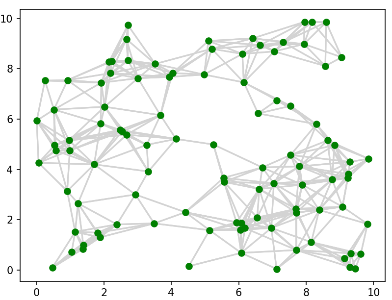
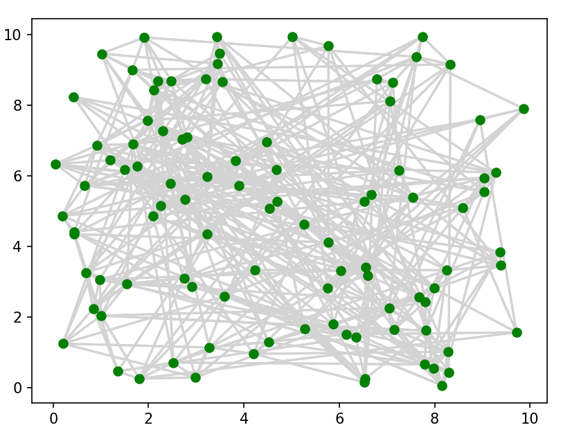
We generalize networks in the numerical experiments from the random geometric graph (RGG) model (Ugander et al.,, 2013). The RGG model is a spatial graph where units are scattered according to a uniform distribution in the region . Two units and are connected if , where is the limiting expected degree of the RGG model. To simulate the long-range dependency, we allow a unit to connect with units outside the radius , which are selected uniformly at random. Figure 1 shows two randomly generated RGG model with different parameters. Furthermore, if and are connected, we assign the weight coefficient independently from a uniform distribution , where . Note that the magnitude of the inference is inversely proportional to the average degree.
To choose the parameters in the exposure mapping model Eq (1), we first generate and independently from for each . We then re-scale the parameters by , and . The re-scaling step ensures that the true baseline parameter, , the direct treatment effect parameter, and the interference effect parameter are , , and , respectively. The true value of the ATE is equal to in all randomly generated instances.
6.2 Comparison of Different Designs
The first design in our test is the fixed-cluster mixed randomization design in Section 3 with known interference weights . In the experiment, we generate the clusters using Algorithm 1 and implement the treatment assignment steps in Section 3.3. The second design is the weight-invariant design described in Section 4, which is agnostic to the weight coefficients . Finally, we test the randomized graph cluster randomization (RGCR) design Ugander and Yin, (2023), which is the state-of-the-art method for cluster-based design. In all designs, we fix the probability of treatment to be . We denote the estimators of the above three designs by , , and , respectively.
To compare the performance under different network sizes and structures, we generate test instances, parameterized by . The network size is chosen from . The value of is chosen from the set . Note that is either 4 or 16, which represents the expected average degree in the RGG model. Recall that when is positive and is zero, units are only connected to those in short distances. When is positive, units may be subject to long-range inference.
We consider three performance metrics for the ATE estimators : mean (), variance (), and theoretical variance upper bounds () given by Proposition 4. For each instance, we run 10,000 independent simulations for each design. The (exact) variances for and are approximated by sample variances, while the variance of the RGCR is calculated according to formula (2.1) to (2.3) in Ugander and Yin, (2023). To calculate theoretical upper bounds on the variance, we use . The variance upper bound for the RGCR design is given by (this bound is in fact tighter than the bound used in Ugander and Yin, (2023)). The simulation results are summarized in Table 1.
| (1000,4,0) | 1.01 | 0.98 | 1.05 | 1.18 | 98.48 | 1.60 | 2.31 | 217.93 | 58.87 |
|---|---|---|---|---|---|---|---|---|---|
| (1000,2,2) | 1.04 | 1.01 | 1.00 | 1.58 | 61.18 | 3.10 | 2.76 | 108.44 | 562.53 |
| (1000,0,4) | 1.03 | 1.00 | 1.03 | 1.81 | 20.84 | 3.47 | 2.98 | 37.15 | 728.85 |
| (1000,16,0) | 1.06 | 1.98 | 0.99 | 6.32 | 1225.79 | 11.36 | 12.69 | 3465.31 | 1910.17 |
| (1000,8,8) | 1.04 | 1.26 | 0.93 | 13.22 | 639.16 | 32.89 | 25.44 | 2267.65 | 53433.22 |
| (1000,0,16) | 1.07 | 0.57 | 0.96 | 15.37 | 507.15 | 45.77 | 30.13 | 2077.55 | 66028.03 |
| (2000,4,0) | 1.01 | 1.53 | 1.01 | 0.64 | 76.97 | 0.85 | 1.20 | 133.91 | 29.18 |
| (2000,2,2) | 1.01 | 1.02 | 1.01 | 0.83 | 42.80 | 1.67 | 1.49 | 80.48 | 330.58 |
| (2000,0,4) | 0.99 | 0.92 | 1.00 | 0.79 | 9.87 | 1.66 | 1.52 | 18.57 | 378.55 |
| (2000,16,0) | 0.97 | 1.29 | 1.03 | 3.53 | 485.21 | 5.71 | 6.79 | 2167.94 | 1066.67 |
| (2000,8,8) | 1.04 | 1.44 | 1.00 | 6.56 | 355.62 | 18.59 | 12.35 | 1419.96 | 57776.42 |
| (2000,0,16) | 1.02 | 0.99 | 1.05 | 7.53 | 254.43 | 26.25 | 15.09 | 1038.87 | 69962.69 |
| (4000,4,0) | 1.01 | 1.36 | 0.97 | 0.34 | 63.24 | 0.41 | 0.64 | 105.77 | 15.44 |
| (4000,2,2) | 1.01 | 0.82 | 0.99 | 0.42 | 33.58 | 0.88 | 0.76 | 59.63 | 193.27 |
| (4000,0,4) | 1.00 | 1.04 | 1.02 | 0.44 | 5.43 | 0.93 | 0.75 | 9.29 | 193.31 |
| (4000,16,0) | 1.02 | 0.97 | 0.98 | 1.85 | 289.58 | 3.27 | 3.63 | 1203.06 | 575.97 |
| (4000,8,8) | 1.00 | 1.10 | 0.97 | 3.25 | 215.23 | 9.68 | 6.42 | 998.78 | 59398.23 |
| (4000,0,16) | 1.00 | 1.12 | 1.05 | 3.91 | 130.46 | 12.15 | 7.63 | 519.46 | 71930.99 |
We have several observations from the results in Table 1. First, let us examine the metrics for (fixed clustering) and (weight-invariant random clustering) under the mixed randomization design. As both estimators are unbiased, we expect that the means will be closer to the ATE when the sample variances are small. This relationship is confirmed by the simulation result. For sample variances , we observe from Table 1 that given , if the network size doubles, sample variances will decrease approximately by a half. Additionally, given , as the limiting expected degree increases, the variances of increase by approximately . These relationships imply that the bound in Theorem 5 is probably tight. We also observe that the theoretical variance upper bounds of from Proposition 4, , is often less than twice the simulated sample variance, , suggesting that the bound in Proposition 4 serves as a good approximation of the true variance.
Next, let us compare the variances of the estimators across all three designs, including for the RGCR cluster-based design (Ugander and Yin,, 2023). The estimator under fixed clustering achieves the smallest sample variance and estimation errors among all three methods. The weight-invariant design () has significantly larger sample variance and estimation errors of the ATE compared to either the fixed-cluster mixed design () or cluster-based design (). This is not surprising as the weight-invariant design assumes unknown edge weights. The fixed-cluster mixed design has a significantly smaller variance upper bound () than the other designs, whereas the upper bound of the RGCR design () is the largest compared to the others. However, empirically, the sample variances of RGCR are much smaller than the theoretical upper bounds, which indicates there might be a gap in the theoretical analysis of RGCR.
Finally, we examine the impact of the network structure parameters and on the performance of these ATE estimators. For each setting or , we consider three values of . Recall that when the average degree () is fixed, a larger indicates that more neighbors are located in short distances, whereas a larger implies more influences from long-range neighbors. Interestingly, we find that the fixed-cluster mixed design is robust across all three cases and the variance barely changes with . The weight-invariant design performs better under long-range interference (i.e., larger ) but performs poorly under local network interference. However, the RGCR performs better with strong local network inference (i.e., larger ).
7 Conclusions
We consider the problem of estimating the average treatment effect when units in an experiment may interfere with other units. The interference pattern is represented by an edge-weighted network, where the weights denote the magnitude of interference between a pair of units. Based on previous literature (Saveski et al.,, 2017; Pouget-Abadie et al., 2019b, ), we propose a mixed experiment design that combines two commonly used methods: cluster-based randomization and Bernoulli randomization. We propose an unbiased estimator for the average treatment effect and establish upper and lower bounds on the variance of this estimator. Both the known edge weights case and the unknown edge weights case are studied. Moreover, we show the consistency and asymptotic normality of the proposed estimator given the network satisfies certain sparsity conditions.
Appendix A Proof of Main Results
A.1 Proof of Proposition 2
Proof.
We introduce the following notations:
Rewrite and , we have
| (13) |
Notice that , , , , and . Plugging these into Eq (13), we have
| (14) |
By Lemma 1 and , we have
| (15) |
Recall that for all and , which implies that for all . Thus,
Furthermore, implies for all . Let , then we have
Finally, let . By Eq (1), we have
| (16) |
Combine all above together and using the fact that , the proof is complete.
∎
A.2 Proof of Proposition 4
Proof.
Note that
Below, we inherit the notations defined in the proof of Proposition 2. Analogous to the proof of Proposition 2, we have
Combining the above equations, we have
Recall that for all and , which implies that for all (here is the treatment for all units other than ). So
Next, consider another clustering of the network where each vertex forms an individual cluster (i.e., ). By inequality (17) in Lemma 13
Then the upper bound in Eq (7) follows. The proof for the lower bound in Eq (8) is almost identical and thus is omitted.
∎
A.3 Proof of Theorem 5
Proof.
The proof includes two steps. Firstly, we would show that under the cluster set generated by maximum weight matching, the approximate variance upper bound defined in (9) is . Since the merging step in Algorithm 1 strictly decrease the value of , we then show that implies the variance of the estimator is also , which completes the proof.
To bound under the cluster set generated by maximum weight matching, we bound , and , respectively. By Lemma 15 in Appendix B, a maximum weight matching guarantees in a graph with maximum degree , thus
To bound , because in the max weight matching and , we have
By Lemma 13, since the maximum cluster size is 2. Combining the upper bounds for , and , defined in (9) is .
Next, we show that implies . We first prove that is an upper bound for . By the assumption that for all and , we have and for all and . Thus
which implies
and therefore,
Then by the variance upper bound in Proposition 4, there exists a positive constant such that
where the second inequality follows from and , and in the third inequality is a constant. ∎
A.4 Proof of Theorem 6
Proof.
Recall that by the definition of Algorithm 2, the size of any cluster is no more than . Let denote the center vertex of a 2-hop cluster in the first step of the algorithm, and be the set of all such vertices. Suppose there exists such that for any , then does not intersect with for any . Otherwise, there exists and a path from to with at most 4 hops, which is a contradiction. Thus for any , for some chosen in the first step of the algorithm.
Suppose and consists of vertices generated from the first step of the algorithm. Since , we have
Thus, we have
where the first inequality follows from the definition of in Eq (6), the second inequality holds since we assume the weights satisfy and , and the final inequality is from the previous equation. This gives an upper bound for .
To bound , we have since . To bound , we apply Lemma 13 and obtain . Combining the upper bounds for , and together and applying Proposition 4, the variance of estimator is .
∎
A.5 Proof of Theorem 7
Proof.
In a -cycle network, we call an edge a Type-1 edge if , and a Type-2 edge if . We say a cluster is continuous if and only if it includes at least edges from the set . Let and be the set of Type-1 and Type-2 edges, respectively.
Consider a cluster of size . Let denote the number of Type- edges () in cluster , i.e. , for . First, we bound as follows:
-
(1-a)
When , since the maximum number of edges in is (when is a clique), we have .
-
(1-b)
When ,
-
(1-c)
When ,
Similarly, for , we have the following bounds:
-
(2-a)
When , we have .
-
(2-b)
When ,
-
(2-c)
When ,
Note that when (i.e., Case 2-b),
so the bound in (2-c) also applies to (2-b).
To summarize,
It’s easy to check that is nonnegative and increasing on . Suppose we have clusters, and is the size of the th cluster. Then by and the Cauchy-Schwarz inequality,
Furthermore, we relax to continuous variables. Note that when , . When , we have
When , . Thus, . Then by Lemma 14, , and the proof is complete.
∎
A.6 Proof of Theorem 12
Proof.
Let , then and . Recall that is defined to be the set of vertices within hops of a vertex in Definition 3. For two units and , if and are not both intersect with any clusters, then and are independent. Using the notation in Lemma 11 and under condition (1), a unit is connected to at most clusters and each cluster is connected to at most nodes, thus . Under condition (2), for unit and any unit , and are independent, thus . Apply Lemma 11 and the result follows.
∎
Appendix B Auxiliary Results
Lemma 13.
We have the following bound for (defined in Proposition 4):
Proof.
Lemma 14.
For any function , if there exists , then the optimal value of the following optimization problem is bounded by
Proof.
The result follows from the following inequality:
∎
Lemma 15.
For a graph with the edge weights and the maximum degree , the sum of weights in a maximum weight matching is at least .
Proof.
Let be the subgraph of induced by a subset of vertices and the subgraph induced by and . For brevity of notations, we let denote the subset of such that each vertex in is incident to at least one edge in . We provide Algorithm 4 based on maximum matching.
The function turns an edge set into a clustering design. If , then and are in the same cluster. If is not covered by , the itself is a cluster. The idea of this algorithm is to decompose the graph into clustering set , such that each edge is covered by exactly one cluster from a specific clustering .
The set represents the uncovered edges. In line 4, we found a vertex set with the largest degree. In line 5, we found a maximum matching from the subgraph , thus an unmatched vertex in cannot be adjacent to another unmatched vertex. In lines 6 to 9, we found edge set such that each vertex in has exactly one edge from incident to it. Also, the edges covered by clustering is exactly . After constructing a clustering from and in line 10, we found the set of vertex without incident to . Since the graph is bipartite and every has the same degree, the maximum matching we found in line 14 is always a perfect matching by Hall’s marriage theorem. Thus, remove , and from will strictly decrease . Since the maximum degree of graph is , the algorithm will terminate after at most while loops. Also, once an edge is covered by a clustering, we directly remove it from the uncovered edge set , making each edge is covered exactly once.
Algorithm 4 decomposes a graph with maximum degree to at most graph matchings, such that each edge in is covered exactly once. This implies that a maximum weight matching under the weights is at least . ∎
References
- Andreev and Räcke, (2004) Andreev, K. and Räcke, H. (2004). Balanced graph partitioning. In Proceedings of the sixteenth annual ACM symposium on Parallelism in algorithms and architectures, pages 120–124.
- Aronow and Samii, (2017) Aronow, P. M. and Samii, C. (2017). Estimating average causal effects under general interference, with application to a social network experiment. The Annuals of Applied Statistics, 11(4):1912–1947.
- Bojinov et al., (2023) Bojinov, I., Simchi-Levi, D., and Zhao, J. (2023). Design and analysis of switchback experiments. Management Science, 69(7):3759–3777.
- Bramoullé et al., (2009) Bramoullé, Y., Djebbari, H., and Fortin, B. (2009). Identification of peer effects through social networks. Journal of econometrics, 150(1):41–55.
- Brennan et al., (2022) Brennan, J., Mirrokni, V., and Pouget-Abadie, J. (2022). Cluster randomized designs for one-sided bipartite experiments. Advances in Neural Information Processing Systems, 35:37962–37974.
- Candogan et al., (2023) Candogan, O., Chen, C., and Niazadeh, R. (2023). Correlated cluster-based randomized experiments: Robust variance minimization. Management Science. (forthcoming).
- Chin, (2019) Chin, A. (2019). Regression adjustments for estimating the global treatment effect in experiments with interference. Journal of Causal Inference, 7(2):20180026.
- Eckles et al., (2016) Eckles, D., Karrer, B., and Ugander, J. (2016). Design and analysis of experiments in networks: Reducing bias from interference. Journal of Causal Inference, 5(1):20150021.
- Galil, (1986) Galil, Z. (1986). Efficient algorithms for finding maximum matching in graphs. ACM Computing Surveys (CSUR), 18(1):23–38.
- Halloran and Struchiner, (1995) Halloran, M. E. and Struchiner, C. J. (1995). Causal inference in infectious diseases. Epidemiology, 6(2):142–151.
- Harshaw et al., (2023) Harshaw, C., Sävje, F., Eisenstat, D., Mirrokni, V., and Pouget-Abadie, J. (2023). Design and analysis of bipartite experiments under a linear exposure-response model. Electronic Journal of Statistics, 17(1):464–518.
- Hudgens and Halloran, (2008) Hudgens, M. G. and Halloran, M. E. (2008). Toward causal inference with interference. Journal of the American Statistical Association, 103(482):832–842.
- Imbens and Rubin, (2015) Imbens, G. W. and Rubin, D. B. (2015). Causal inference in statistics, social, and biomedical sciences. Cambridge University Press.
- Johari et al., (2022) Johari, R., Li, H., Liskovich, I., and Weintraub, G. Y. (2022). Experimental design in two-sided platforms: An analysis of bias. Management Science, 68(10):7069–7089.
- (15) Leung, M. P. (2022a). Causal inference under approximate neighborhood interference. Econometrica, 90(1):267–293.
- (16) Leung, M. P. (2022b). Rate-optimal cluster-randomized designs for spatial interference. The Annals of Statistics, 50(5):3064–3087.
- Li and Wager, (2022) Li, S. and Wager, S. (2022). Network interference in micro-randomized trials. arXiv preprint arXiv:2202.05356.
- Manski, (2013) Manski, C. F. (2013). Identification of treatment response with social interactions. The Econometrics Journal, 16(1):S1–S23.
- Paluck et al., (2016) Paluck, E. L., Shepherd, H., and Aronow, P. M. (2016). Changing climates of conflict: A social network experiment in 56 schools. Proceedings of the National Academy of Sciences, 113(3):566–571.
- (20) Pouget-Abadie, J., Aydin, K., Schudy, W., Brodersen, K., and Mirrokni, V. (2019a). Variance reduction in bipartite experiments through correlation clustering. Advances in Neural Information Processing Systems, 32.
- (21) Pouget-Abadie, J., Saint-Jacques, G., Saveski, M., Duan, W., Ghosh, S., Xu, Y., and Airoldi, E. M. (2019b). Testing for arbitrary interference on experimentation platforms. Biometrika, 106(4):929–940.
- Ross, (2011) Ross, N. (2011). Fundamentals of Stein’s method. Probability Surveys, 8:210–293.
- Saveski et al., (2017) Saveski, M., Pouget-Abadie, J., Saint-Jacques, G., Duan, W., Ghosh, S., Xu, Y., and Airoldi, E. M. (2017). Detecting network effects: Randomizing over randomized experiments. In Proceedings of the 23rd ACM SIGKDD international conference on knowledge discovery and data mining, pages 1027–1035.
- Sävje, (2023) Sävje, F. (2023). Causal inference with misspecified exposure mappings: separating definitions and assumptions. Biometrika, page asad019.
- Sävje et al., (2021) Sävje, F., Aronow, P., and Hudgens, M. (2021). Average treatment effects in the presence of unknown interference. Annals of statistics, 49(2):673.
- Tchetgen and VanderWeele, (2012) Tchetgen, E. J. T. and VanderWeele, T. J. (2012). On causal inference in the presence of interference. Statistical methods in medical research, 21(1):55–75.
- Toulis and Kao, (2013) Toulis, P. and Kao, E. (2013). Estimation of causal peer influence effects. In International conference on machine learning, pages 1489–1497. PMLR.
- Ugander et al., (2013) Ugander, J., Karrer, B., Backstrom, L., and Kleinberg, J. (2013). Graph cluster randomization: Network exposure to multiple universes. In Proceedings of the 19th ACM SIGKDD international conference on Knowledge discovery and data mining, pages 329–337.
- Ugander and Yin, (2023) Ugander, J. and Yin, H. (2023). Randomized graph cluster randomization. Journal of Causal Inference, 11(1):20220014.