Differentially Private Functional Summaries via
the Independent Component Laplace Process

Abstract

In this work we propose a new mechanism for releasing differentially private functional summaries called the Independent Component Laplace Process, or ICLP, mechanism. By treating the functional summaries of interest as truly infinite-dimensional objects and perturbing them with the ICLP noise, this new mechanism relaxes assumptions on data trajectories and preserves higher utility compared to classical finite-dimensional subspace embedding approaches in the literature. We establish the feasibility of the proposed mechanism in multiple function spaces. Several statistical estimation problems are considered, and we demonstrate by slightly over smoothing the summary, the privacy cost will not dominate the statistical error and is asymptotically negligible. Numerical experiments on synthetic and real datasets demonstrate the efficacy of the proposed mechanism.

Keywords: Differential Privacy, Functional Data Analysis, Hilbert Space, Reproducing Kernel Hilbert Space, Stochastic Processes,

1 Introduction

Data security has garnered critical attention in the last decade as substantial individualized data are collected. The most widely used paradigm in formal data privacy is differential privacy (DP), introduced by Dwork et al. (2006). DP provides a rigorous and interpretable definition for data privacy as it bounds the amount of information that attackers can infer from publicly released database queries. Numerous mechanisms have been developed under conventional data settings like scalar or vector-valued data. However, advances in technologies enable us to collect and process densely observed data over some temporal or spatial domains, which are coined functional data to differentiate them from classic multivariate data (Ramsay et al., 2005; Kokoszka and Reimherr, 2017; Ferraty and Romain, 2011). Even though functional data analysis, FDA, has been proven useful in various fields like economics, finance, genetics and etc., and has been researched widely in the statistical community, there are only a few works concerning privacy preservation within the realm of functional data.

In this paper, we propose an additive noise mechanism for functional summaries, namely infinite dimensional summaries, to achieve $\epsilon$-DP. Additive noise mechanisms are one of the most commonly used mechanisms to achieve DP, which sanitizes statistical summaries by adding calibrated noise from predetermined distributions, e.g. Laplace and Gaussian mechanism (Dwork et al., 2006, 2014). With functional summaries, classic privacy tools embed the problem into a finite-dimensional subspace by using finite basis expansions to approximate summaries and perturb expansion coefficients with i.i.d. noise (Wang et al., 2013; Chandrasekaran et al., 2014; Alda and Rubinstein, 2017; Zhang et al., 2012). However, these mechanisms have potential weaknesses. First, determining the dimension of the subspace is crucial as it plays a trade-off role between utility and privacy. While data-driven approaches might cause potential privacy leakage, a pre-determined dimension will lack adaption to the data, potentially failing to capture the shape of the functions or injecting excess noise. Second, in multivariate settings, privacy budget allocation over each component can affect a mechanism’s utility and robustness substantially. Some previous work has shown that capturing the covariance structure in the data can substantially reduce the amount of noise injected (Hardt and Talwar, 2010; Awan and Slavković, 2021). However, current mechanisms allocate an equal privacy budget to all components, failing to recognize the importance of different functional components, and thus injecting excess noise for “more important” components, degrading utility and robustness.

Contribution: To overcome the downsides inherent in finite-dimensional subspaces embedding approaches, we treat the functional summary and privacy noise as truly infinite-dimensional. We propose a mechanism by perturbing functional summaries with a stochastic process called the Independent Component Laplace Process (ICLP), and name this mechanism as the ICLP mechanism. It ensures a full path-level release rather than a finite grid of evaluating points. We establish the feasibility of the ICLP mechanism in a general separable Hilbert space, $\mathbb{H}$, by characterizing a subspace of $\mathbb{H}$ and show that the feasibility holds if and only if functional summaries reside in this subspace. We also show how the proposed mechanism applies to the space of the continuous functions, even though this space is not a Hilbert space. We provide two strategies based on regularization to restrict the functional summaries to be within a desired subspace and show one can gain privacy for “free” by slightly over smooth the summaries. We demonstrate the proposed mechanism for the mean function protection problem and show it can go beyond classic functional data settings, as it is also applicable to the realm of more classic non-parametric smoothing problems like kernel density estimation. To obtain a privacy-safe regularization parameter in the regularization term, we adopt the plug-in approach such that the regularization parameters are tied to the covariance structure of the ICLP noise. This approach not only overcomes the potential information leakage in conventional data-driven approaches, but also has theoretical utility guarantees. The proposed mechanism differentiates itself from current mechanisms in the following senses. First, the ICLP mechanism avoids finite-dimensional subspace embeddings and frees the assumption that every dataset in the database shares the same finite-dimensional subspace. Second, the privacy budgets allocated to each component are not uniform but proportional to the global sensitivity of that component. Compared to uniform allocation in current mechanisms, like the functional mechanism (Zhang et al., 2012) and Bernstein mechanism (Alda and Rubinstein, 2017), such allocation injects less noise into the more important components, which improves the utility of the released summaries.

Related Work: In the overlap of functional summaries and differential privacy, the landmark paper is Hall et al. (2013) which provided a framework for achieving $(\epsilon,\delta)$-DP on infinite dimensional functional objects, but focussed on a finite grid of evaluation points. The follow-up work in Mirshani et al. (2019) pushed Hall et al. (2013)’s result forward, established $(\epsilon,\delta)$-DP over the full functional path for objects in Banach spaces. In more general spaces, Reimherr and Awan (2019) considered elliptical perturbations to achieve $(\epsilon,\delta)$-DP in locally convex vector spaces, including all Hilbert spaces, Banach spaces, and Frechet spaces. They also showed the impossibility of achieving $\epsilon$-DP in infinite dimensional objects with elliptical distributions.

Turning to $\epsilon$-DP, a series of works have been proposed by resorting to finite-dimensional representations, like polynomial bases, trigonometric bases, or Bernstein polynomial bases to approximate target functional summaries (Wang et al., 2013; Chandrasekaran et al., 2014; Alda and Rubinstein, 2017) and loss functions (Zhang et al., 2012). One then perturbs the expansion coefficients via the Laplace mechanism independently. In addition to additive noise mechanisms, Awan et al. (2019) extended the exponential mechanism (McSherry and Talwar, 2007) to any arbitrary Hilbert spaces and showed its application to functional principal component analysis. From the perspective of the robust noise injection, a heterogeneous noise injection scheme (Phan et al., 2019) is proposed by assigning different weighted privacy budgets on each coordinate to further improve the robustness of private summaries.

2 Preliminaries and Notation

2.1 Differential Privacy

Let $\mathcal{D}$ be the collection of all possible $n$-unit databases and $D$ be an element of $\mathcal{D}$. Denote the summary of interest as $f:\mathcal{D}\to\Omega$, where $(\Omega,\mathcal{F})$ is a measurable space. We denote the sanitized version of $f_{D}$ by $\tilde{f}_{D}$, which is a random element of $\Omega$ indexed by $D$. We state the definition of differential privacy in terms of conditional distributions (Wasserman and Zhou, 2010).

Definition 1

Let $\tilde{f}_{D}$ be the sanitized version of the functional summary $f_{D}$. Assume $\{P_{D}:D\in\mathcal{D}\}$ is the family of probability measures over $\Omega$ induced by $\{\tilde{f}_{D}:D\in\mathcal{D}\}$. We say $\tilde{f}_{D}$ achieves $\epsilon$-DP if for any two adjacent datasets (only different on one record) $D,D^{\prime}$, and any measurable set $A\in\mathcal{F}$, one has

$$P_{D}(A)\leq e^{\epsilon}P_{D^{\prime}}(A).$$

The definition implies the summaries of two adjacent datasets should have almost the same probability distribution. The privacy budget $\epsilon$ controls how much privacy will be lost while releasing the result, and a small $\epsilon$ implies a higher similarity between $P_{D}$ and $P_{D^{\prime}}$ and thus increased privacy.

2.2 Notation

We introduce some notation that will be used now throughout the paper. Let $\mathbb{H}$ be a real separable Hilbert space with inner product $\langle\cdot,\cdot\rangle_{\mathbb{H}}$. A random element $X\in\mathbb{H}$ is said to have mean $\mu\in\mathbb{H}$ and (linear) covariance operator $C:\mathbb{H}\to\mathbb{H}$ if

$$\operatorname{E}[\langle X,h\rangle_{\mathbb{H}}]=\langle\mu,h\rangle_{\mathbb{H}}\qquad\text{and}\qquad\operatorname{Cov}(\langle X,h_{1}\rangle_{\mathbb{H}},\langle X,h_{2}\rangle_{\mathbb{H}})=\langle Ch_{1},h_{2}\rangle_{\mathbb{H}},$$

for any $h,h_{1},h_{2}$ in $\mathbb{H}$. A linear operator, $C$, is a covariance operator if and only if it is symmetric, positive semidefinite, and trace class (Bosq, 2000). Denoted $\{\lambda_{j},\phi_{j}\}_{j\geq 1}$ as the eigenvalues and eigenfunctions of C, then we define two norms associated with $C$:

$$\left\|h\right\|_{C}=\sqrt{\sum_{j\geq 1}\frac{\langle h,\phi_{j}\rangle_{\mathbb{H}}^{2}}{\lambda_{j}}}\quad\textit{and}\quad\left\|h\right\|_{1,C}=\sum_{j\geq 1}\frac{|\langle h,\phi_{j}\rangle_{\mathbb{H}}|}{\sqrt{\lambda_{j}}}.$$

We also denote the two corresponding subspaces of $\mathbb{H}$ as $\mathbb{H}_{C}=\{h\in\mathbb{H}:\|h\|_{C}<\infty\}$ and $\mathbb{H}_{1,C}=\{h\in\mathbb{H}:\|h\|_{1,C}<\infty\}$. Note $\left\|\cdot\right\|_{C}$ is the classic Cameron-Martin norm induced by $C$ (Bogachev, 1998) and $\mathbb{H}_{C}$ is called the Cameron-Martin space of $C$. Here $\left\|\cdot\right\|_{1,C}$ is analogous to a weighted $\ell^{1}$-norm, and $h\in\mathbb{H}_{1,C}$ leads to $h\in\mathbb{H}_{C}$. Lastly, we will use some common notation when discussing asymptotic results, namely, let $a_{n}\asymp b_{n}$ and $a_{n}\lesssim b_{n}(a_{n}=O(b_{n}))$ denote $|a_{n}/b_{n}|\rightarrow c$ and $|a_{n}/b_{n}|\leq c$, respectively, for some constant $c$ when $n\rightarrow\infty$.

3 The ICLP Mechanism and its Feasibility

In this section, we first define the Independent Component Laplace Process, and then formally propose the the ICLP mechanism, where the private summary takes the form of $\tilde{f}_{D}=f_{D}+\sigma Z$ with $Z$ as an ICLP noise. Initially, we assume $f_{D}$ lies in a real separable Hilbert space $\mathbb{H}$. Then we also show that privacy protection can also hold for the space of continuous functions (which is not a Hilbert space) as well under certain assumptions on the covariance operator. The proofs of all the Lemmas and Theorems can be found in Appendix A.

3.1 Independent Component Laplace Process

The proposed stochastic process is motivated by Mirshani et al. (2019), who achieved $(\epsilon,\delta)$-DP on functional summaries in Banach spaces. Formally, their mechanism can be written as $\tilde{f}_{D}=f_{D}+\sigma Z$ where $Z\sim GP(0,C)$ is a centered Gaussian process with covariance operator $C$. There is a dual perspective of this mechanism. By applying the Karhunen-Loéve Theorem (Kosambi, 2016), the mechanism is equivalent to

$$\tilde{f}_{D}=f_{D}+\sigma Z=\sum_{j=1}^{\infty}\left(\left\langle f_{D},\phi_{j}\right\rangle+\sigma\left\langle Z,\phi_{j}\right\rangle\right)\phi_{j},$$ (1)

where $\{\lambda_{j}\}_{j\geq 1}$ and $\{\phi_{j}\}_{j\geq 1}$ are the eigenvalues and eigenfunctions of $C$ and $\langle Z,\phi_{j}\rangle$ independently follows $N(0,\lambda_{j})$, meaning that the mechanism perturbs each component’s coefficient with independent normal random variables. Unfortunately, the existing Laplace process cannot play a role analogous to the Gaussian process under such an expansion since it is an elliptical distribution and it has been proved that no elliptical distribution can be used to achieve $\epsilon$-DP in infinite-dimensional spaces (Reimherr and Awan, 2019). Motivated by the dual perspective from the Karhunen-Loéve expansion and the Laplace mechanism in the scalar setting, we consider adding independent Laplace noises with heterogeneous variances in the expansion (1), which is equivalent to perturbing the functional summary with a particular stochastic process. The desired stochastic process is defined as follows.

Definition 2

Let $X$ be a random element in $\mathbb{H}$ with $\operatorname{E}\|X\|^{2}<\infty$. Given a non-negative decreasing real sequence, $\{\lambda_{j}\}_{j\geq 1}$, satisfying $\sum_{j\geq 1}\lambda_{j}<\infty$, and an orthonormal basis of $\mathbb{H}$, $\{\phi_{j}\}_{j\geq 1}$, we say $X$ is an Independent Component Laplace Process with mean $\mu$ if it admits the decomposition

$$X=\mu+\sum_{j=1}^{\infty}\sqrt{\lambda_{j}}Z_{j}\phi_{j},$$

where $Z_{j}$ are i.i.d. Laplace random variables with zero-mean and variance $1$.

The collection of square integrable random elements of $\mathbb{H}$ is itself a Hilbert space with inner product $\operatorname{E}\langle X,Y\rangle_{\mathbb{H}}$. Thus, while the ICLP is given as an infinite sum, it is still well-defined, see Chapter 1 in Bosq (2000).

Theorem 3

If the given non-negative decreasing real sequence, $\{\lambda_{j}\}_{j\geq 1}$, satisfies $\sum_{j\geq 1}\lambda_{j}<\infty$, and the basis $\{\phi_{j}\}_{j\geq 1}$ are orthonormal in $\mathbb{H}$, then the stochastic process defined in Definition 2 is well-defined in $\mathbb{H}$.

3.2 Feasibility in Separable Hilbert Spaces

To investigate the feasibility of a randomized mechanism, one can start with the equivalence/orthogonality of probability measures. As discussed in Awan et al. (2019) and Reimherr and Awan (2019), the probability measures induced by an $\epsilon$-DP mechanism are necessarily equivalent (though this is not sufficient for DP) in a probabilistic sense; otherwise, it is impossible to be DP if the measures are orthogonal. More specifically, if the mechanism produces a private summary $\tilde{f}_{D}$ that is probabilistically orthogonal to $\tilde{f}_{D^{\prime}}$, i.e. there exists a $A\in\mathcal{F}$ so that $P_{D}(A)=0$ and $P_{D^{\prime}}(A)=1$, then the mechanism cannot be DP since $f_{D}$ and $f_{D^{\prime}}$ can be distinguished with probability one on $A$. In the following, we use this perspective to develop the feasibility of the ICLP mechanism. Denote the probability measure family induced by the ICLP mechanism as $\{P_{D}:D\in\mathcal{D}\}$, in the following theorem, we provide necessary and sufficient conditions for pairwise equivalence in $\{P_{D}:D\in\mathcal{D}\}$.

Theorem 4

Let $D,D^{\prime}\in\mathcal{D}$ be two adjacent datasets, $\tilde{f}_{D},\tilde{f}_{D^{\prime}}$ be the private summaries based on the ICLP mechanism, and denote the corresponding probability measures over $\mathbb{H}$ as $P_{D}$ and $P_{D^{\prime}}$. Then $P_{D}$ and $P_{D^{\prime}}$ are equivalent if and only if

$$f_{D}-f_{D^{\prime}}\in\mathcal{H}_{C}=\left\{h\in\mathbb{H}:\|h\|_{C}<\infty\right\}.$$ (2)

Theorem 4 shows that if the difference of $f_{D}$ and $f_{D^{\prime}}$ resides in the Cameron-Martin space of $C$ then the probability family will be pairwise equivalent. An analogous result for the equivalence of elliptical distributions appears in Theorem 2 of Reimherr and Awan (2019) even though the ICLP is not an elliptical distribution. However, it turns out that, unlike elliptical distributions, pairwise equivalence is not enough for the ICLP mechanism to achieve DP. To see the reason behind this, one needs to consider the density of $P_{D}$ in $\mathbb{H}$. Since there is no common base measure in $\mathbb{H}$ that plays the same role as the Lebesgue measure in $\mathbb{R}^{d}$, it is more complicated to consider the density in $\mathbb{H}$. Fortunately, we are adding the same type of noise to functional summaries, and therefore we only need the density as the Radon-Nikodym derivative of $P_{D}$ w.r.t. $P_{0}$, where $P_{0}$ is the probability measure induced by $\sigma Z$.

Lemma 5

Let $P_{h}$ and $P_{0}$ be the probability measures induced by $\{h+\sigma Z\}$ and $\sigma Z$. Suppose $h\in\mathcal{H}_{C},$ then the Radon–Nikodym derivative of $P_{D}$ w.r.t. $P_{0}$ is given by

$$\frac{dP_{h}}{dP_{0}}(z)=exp\left\{-\frac{1}{\sigma}\left(\left\|z-h\right\|_{1,C}-\left\|z\right\|_{1,C}\right)\right\},$$ (3)

$P_{0}$ almost everywhere and is unique.

Now we are ready to show why Condition (2) is not enough for $\epsilon$-DP. Indeed, the pairwise equivalence only guarantees the density in Equation (3) is well-defined, but does not guarantee that the density is bounded, which is a requirement for $\epsilon$-DP however. Meanwhile, $\mathcal{H}_{C}$ is enough for $(\epsilon,\delta)$-DP since it allows densities to be unbounded up to a set with $P_{0}$ measure less than $\delta$. In the next theorem, we will show the appropriate space that $f_{D}-f_{D^{\prime}}$ should reside in is actually a subspace of $\mathcal{H}_{C}$.

Theorem 6

Under the same conditions of Theorem 4, let

$$\mathcal{H}_{1,C}=\left\{f\in\mathbb{H}:\|f\|_{1,C}<\infty\right\}$$

be a subspace of $\mathcal{H}_{C}$ and if

$$f_{D_{1}}-f_{D_{2}}\in\mathcal{H}_{C}\setminus\mathcal{H}_{1,C},$$

then there is no $\sigma\in\mathbb{R}^{+}$ such that the ICLP mechanism, $\tilde{f_{D}}=f_{D}+\sigma Z$ satisfies $\epsilon$-DP.

Indeed, if $f_{D}$ resides in the gap between $\mathcal{H}_{C}$ and $\mathcal{H}_{1,C}$, the sensitivity of $f_{D}$ will be infinite and there is no possibility to calibrate the ICLP noise with any $\sigma$ to achieve $\epsilon$-DP. Now, with the proper space in Theorem 6 and the feasible density in Lemma 5, we can establish the ICLP mechanism formally.

Theorem 7 (The ICLP Mechanism)

Let $f_{D}\in\mathcal{H}_{1,C}$ be the functional summary and $Z$ is an ICLP with covariance operator $C$. Define the global sensitivity (GS) as

$$\Delta=\sup_{D\sim D^{\prime}}\|f_{D}-f_{D^{\prime}}\|_{1,C}\quad\textit{and}\quad\sigma=\frac{\Delta}{\epsilon}.$$ (4)

Then the sanitized version of $f_{D}$, $\tilde{f}_{D}=f_{D}+\sigma Z$, achieves $\epsilon$-DP.

3.3 Extensions To Space of Continuous Functions

Theorem 7 implies the ICLP mechanism provides privacy protection for a wide range of infinite-dimensional objects in separable Hilbert spaces. The DP post-processing inequality (Dwork et al., 2014), is an especially important property for functions since practically one may only be interested in a few scalar summaries. However, the post-processing inequality only applies to measurable mappings. If $\mathbb{H}=L^{2}[0,1]$, then this eliminates the possibility of releasing point-wise evaluations of the functional summary, since such mappings are not measurable operations in $L^{2}[0,1]$. Therefore, in this section, we extend the ICLP mechanism to the space of continuous functions, i.e. $\mathcal{C}(T)$ with $T$ a compact set over $\mathbb{R}^{d}$, where such operations are measurable (and thus protected). We show that the ICLP, under mild conditions, is also in $\mathcal{C}(T)$.

Theorem 8

Let $C:T\times T\to\mathbb{R}$ be a symmetric, positive definite, bivariate function with compact domain $T$. If $C$ is $\alpha$-Hölder continuous in each coordinate, i.e. there exists a positive constant $M_{C}$, $\alpha\in(0,1]$ s.t. $\left|C\left(t_{1},s\right)-C\left(t_{2},s\right)\right|\leq M_{C}\left|t_{1}-t_{2}\right|^{\alpha}$ then there exists an ICLP, $Z$, with covariance function $C$ and there exists a modification $\tilde{Z}:T\times\Omega\rightarrow\mathbb{R}$ of $Z$ that is a continuous process, s.t.

1. $\tilde{Z}$ is sample continuous, i.e. $\forall\omega\in\Omega$, $\tilde{Z}_{\omega}(t)$ is continuous w.r.t. $t\in T$;

2. For any $t\in T$, $P(\tilde{Z}(t)=Z(t))=1$.

Meaning that there exists a stochastic process in $\mathcal{C}(T)$ equally distributed as the ICLP except on a zero-measure set.

All of the results of the ICLP mechanism for $\mathbb{H}$ in Section 3.2 are now applicable to summaries in $\mathcal{C}(T)$. Furthermore, the point-wise evaluation is now a measurable operation and thus is protected. We also note that the proof of Theorem 8 is not just a standard theorem from stochastic processes and relies heavily on the structure of the ICLP.

4 Methodology

Based on Theorem 6 and 7, to achieve $\epsilon$-DP one would need to guarantee the quantity, $f_{D}-f_{D^{\prime}}$ lies in $\mathcal{H}_{1,C}$ for any neighboring databases $D$ and $D^{\prime}$. This is a challenging task to do directly and it is easier to structure the problem by restricting the individual functional summary residing in $\mathcal{H}_{1,C}$, which automatically leads to $f_{D}-f_{D^{\prime}}\in\mathcal{H}_{1,C}$. In the rest of this section, we will provide different approaches to construct qualified summaries and derive upper bounds for their global sensitivity. We also apply the ICLP mechanism to achieve privacy protection over several statistical estimation problems.

4.1 Generalized Obtainment of Qualified Summaries

IID Laplace: The first strategy utilizes a finite basis expansion (Kokoszka and Reimherr, 2017) and adds IID Laplace noise to each coefficient, which is in the same spirit as all current mechanisms, which rely on finite-dimensional representations. Let $\{e_{j}\}_{j\geq 1}$ be an orthonormal basis in $\mathbb{H}$. Then we approximate the summary using $M$ bases, i.e.

$$\hat{f}_{D}=\sum_{j=1}^{M}f_{Dj}e_{j}\quad\textit{with}\quad f_{Dj}=\langle f_{D},e_{j}\rangle.$$

Expanding the functional summaries via a finite basis facilitates dimension reduction so that classic privacy tools can be implemented to sanitize each coefficient. Since the functional summary resides in a finite-dimensional subspace, it naturally satisfies the requirement in Theorem 7 (here one takes $\phi_{j}=e_{j}$ and $\lambda_{j}=1$) and therefore leads to a finite GS. However, it inherits all the drawbacks from subspace embedding mechanisms. For example, even though the leading components are usually more important for the utility of the estimate, this approach treats all components equally during the privatizing process and thus degrades the utility of the released summary. Additionally, the truncation level $M$ controls the trade-off between variance, bias, and privacy; this approach would force one to either introduce more noise or accept higher bias when more components are required to deal with complex sample trajectories.

$\boldsymbol{\ell}^{1}$ Regularization: To satisfy $f_{D}\in\mathcal{H}_{1,C}$ while avoiding a finite-dimensional representation, we consider using a regularization approach with $\|\cdot\|_{1,C}$ as a penalty term. Formally, let $L(f,D):\mathbb{H}\times\mathcal{D}\to\mathbb{R}$ be a loss function, consider the following minimization problem,

$$\hat{f}_{D}=\underset{f\in\mathbb{H}}{\operatorname{argmin}}\left\{L(f,D)+\psi\left\|f\right\|_{1,C^{\eta}}\right\}\quad\textit{for}\ \eta\geq 1,$$ (5)

where $C^{\eta}$ shares the same eigenfunctions as $C$ while the eigenvalues are raised to $\lambda_{j}^{\eta}$ and $\psi$ is the regularization parameter. The benefit of using a power of the kernel, $C^{\eta}$, are twofold. First, the space corresponding to $\|\cdot\|_{1,C^{\eta}}$ is a subspace of $\mathcal{H}_{1,C}$, guaranteeing that $\hat{f}_{D}\in\mathcal{H}_{1,C}$. Second, it allows more flexibility to control the smoothness of the constructed functional summaries. Late on, we will see even though $\eta=1$ is a natural setting, a slightly over-smoothing summary can be helpful for utility and even make privacy error negligible compared to statistical error.

RKHS Regularization: As we will see in Section 4.2, there are some serious drawbacks to using the $\|\cdot\|_{1,C}$-norm as the penalty. We, therefore, consider an RKHS approach as our final strategy, which turns out to work quite well in our applications. Formally, for a given $\eta>1$, by the Cauchy-Schwarz inequality,

$$\|h\|_{1,C}=\sum_{j=1}^{\infty}\frac{|h_{j}|}{\sqrt{\lambda_{j}}}=\sum_{j=1}^{\infty}\frac{|h_{j}|}{\lambda_{j}^{\frac{\eta}{2}}}\lambda_{j}^{\frac{\eta-1}{2}}\leq\left\|h\right\|_{C^{\eta}}\sqrt{\operatorname{trace}(C^{\eta-1})}.$$

Therefore, by taking $\eta>1$ such that $C^{\eta-1}$ is a trace-class operator, we get that $\hat{f}_{D}\in\mathcal{H}_{1,C}$ where

$$\hat{f}_{D}=\underset{f\in\mathbb{H}}{\operatorname{argmin}}\left\{L(f,\mathcal{D})+\psi\left\|f\right\|_{C^{\eta}}^{2}\right\}\quad\textit{for}\ \eta>1.$$ (6)

4.2 Mean Function Privacy Protection

In this part, we consider the problem of protecting the privacy of the mean function summary. Assume $X_{1},X_{2},\cdots,X_{n}$ are i.i.d. elements of an arbitrary real separable Hilbert space $\mathbb{H}$ with $\operatorname{E}X_{i}=\mu_{0}\in\mathbb{H}$. Our goal is to release a differentially private estimator of the true mean function $\mu_{0}$ that satisfies $\epsilon$-DP.

When using IID Laplace, one can start with $\hat{f}_{D}=\frac{1}{n}\sum_{i=1}^{n}X_{i}$, which is an unbiased estimator of the mean function $\mu$. While in the other two approaches we use a quadratic loss function in a regularized empirical risk minimization setup with penalty term $P(\theta)=\left\|\theta\right\|_{1,C^{\eta}}$ or $\left\|\theta\right\|_{C^{\eta}}^{2}$, i.e.,

$$\hat{\mu}_{D}=\underset{\theta\in\mathbb{H}}{\operatorname{argmin}}\left\{\frac{1}{n}\sum_{i=1}^{n}\left\|X_{i}-\theta\right\|^{2}+\psi P(\theta)\right\}.$$ (7)

In Theorem 9 and Theorem 11, we derive the close form of the estimators and provide their global sensitivity analysis for $\ell^{1}$ and RKHS regularization.

Theorem 9 ($\ell^{1}$ regularization)

Let $P(\theta)=\|\theta\|_{1,C^{\eta^{l}}}$, then solution of (7) is

$$\hat{\mu}_{D}^{l}=\sum_{j=1}^{\infty}s_{\psi,2\lambda_{j}^{\eta_{l}/2}}\left(\left\langle\bar{X},\phi_{j}\right\rangle\right)\phi_{j}.$$ (8)

where $s_{a,b}(x)=\operatorname{sgn}(|x|)\left(|x|-a/b\right)^{+}$ is the soft thresholding function with threshold $a/b$. Furthermore, assume $\|X\|_{L^{2}}\leq\tau$, then for any fixed $\psi$, there exists an integer $J_{\tau,\psi}$ such that the global sensitivity of $\hat{\mu}_{D}^{l}$ satisfies

$$\sup_{D\sim D^{\prime}}\|\hat{\mu}_{D}^{l}-\hat{\mu}_{D^{\prime}}^{l}\|_{1,C}\leq\frac{2\tau}{n}\sum_{j=1}^{J_{\tau,\psi}}\lambda_{j}^{-\frac{\eta_{l}}{2}},$$

Remark 10

The integer $J_{\tau,\psi}:=\operatorname{max}\{j\geq 1:\tau\leq\psi/\lambda_{j}^{\eta_{l}/2}\}$ indeed can be viewed as a truncation number as the coefficients after $J_{\tau,\phi}$ will be shrunk to $0$, i.e. the summation in (8) is indeed finite. The upper bound for global sensitivity is based on the fact that, in the worst case scenario, the coefficients are not shrunk to zero and thus the soft thresholding adjustments cancel out. Therefore, unfortunately, the $\ell^{1}$ regularization doesn’t produce a better sensitivity than the IID Laplace approach while the soft thresholding introduces extra bias into the summary.

In the next theorem, we show that the RKHS regularized estimator is indeed infinite-dimensional and has a better sensitivity than the other two.

Theorem 11 (RKHS regularization)

Let $P(\theta)=\|\theta\|_{C^{\eta^{r}}}$, then solution of (7) is

$$\hat{\mu}_{D}^{r}=\sum_{j=1}^{\infty}\frac{\lambda_{j}^{\eta_{r}}}{\lambda_{j}^{\eta_{r}}+\psi}\left\langle\bar{X},\phi_{j}\right\rangle\phi_{j}.$$ (9)

Furthermore, assume $\|X\|_{l_{1}}:=\sum_{j\geq 1}|\langle X,\phi_{j}\rangle|\leq\tau$, then the global sensitivity of $\hat{\mu}_{D}^{r}$ satisfies

$$\sup_{D\sim D^{\prime}}\|\hat{\mu}_{D}^{r}-\hat{\mu}_{D^{\prime}}^{r}\|_{1,C}\leq\frac{2\tau}{n}\sup_{j}\left\{\frac{\lambda_{j}^{\eta_{r}-\frac{1}{2}}}{\lambda_{j}^{\eta_{r}}+\psi}.\right\}$$

Remark 12

The coefficients of the RKHS regularized estimator (9) will not be shrunk exactly to zero, and hence one is able to perturb the functional summary with the truly infinite-dimensional ICLP. Besides, other assumptions about the boundness of $X$ can also be used, such as $\|X_{i}\|\leq\tau$, but they in general produce a substantially larger sensitivity.

In the next Theorem, we provide a guarantee of the utility of the ICLP mechanism. We demonstrate that with some smoothness assumptions on the true mean function $\mu_{0}$ and non-private estimator $\hat{\mu}_{D}$, the privacy cost, $\operatorname{E}\|\tilde{\mu}_{D}-\hat{\mu}_{D}\|_{L^{2}}^{2}$, will not dominate the total error, which will be $O(n^{-1})$ and thus matches the optimal rate without privacy. Therefore, one can restrict the summary into a smoother class such that privacy is gained for “free”.

Theorem 13 (Utility Analysis)

Assume $X_{i}$ are i.i.d. observations from $X$ with mean function $\mu_{0}$ and $L^{2}$-norm bounded by $\tau$, $\lambda_{j}\asymp j^{-2\nu}$.

1. Let $\tilde{\mu}_{D}^{r}$ be the private summary from RKHS regularization, if $\|\mu_{0}\|_{C^{\eta_{r}}}<\infty$ then

   $$\operatorname{E}\left\|\tilde{\mu}_{D}^{r}-\mu_{0j}\right\|_{L^{2}}^{2}=O\left(\psi^{-\frac{1}{\eta_{r}}}\left(\frac{\tau}{n\epsilon}\right)^{2}+\frac{1}{n}+\psi\right).$$

   Taking $\eta_{r}\geq 1+(2\nu)^{-1}$ and $\left(\frac{n\epsilon^{2}}{\tau^{2}}\right)^{-\eta_{r}}\lesssim\psi\lesssim n^{-1}$,

   $$\operatorname{E}\left\|\tilde{\mu}_{D}^{r}-\hat{\mu}\right\|_{L^{2}}^{2}=\left\{\begin{aligned} &o(n^{-1}),&\eta_{r}>1+(2\nu)^{-1}\\ &O(n^{-1}),&\eta_{r}=1+(2\nu)^{-1}\end{aligned}\right..$$

2. Let $\tilde{\mu}_{D}^{l}$ be the private summary from $\ell^{1}$ regularization, let $J_{\tau}:=\operatorname{max}\{j\geq 1:\tau\leq\psi/\lambda_{j}^{\eta_{l}/2}\}$. If $\|\mu_{0}\|_{C^{\eta_{l}}}<\infty$

   $$\operatorname{E}\left\|\tilde{\mu}_{D}^{l}-\mu_{0}\right\|_{L^{2}}^{2}=O\left(J_{\tau}^{2(r+1)}\left(\frac{\tau}{n\epsilon}\right)^{2}+\frac{1}{n}+\psi\right).$$

   Taking $\eta_{l}\geq 2(1+\nu^{-1})$ and $\tau^{-\frac{(\eta_{l}-1)\nu-1}{\nu+1}}(\epsilon^{2}n)^{-\frac{\eta_{l}\nu}{2(\nu+1)}}\lesssim\psi\lesssim n^{-1}$,

   $$\operatorname{E}\left\|\tilde{\mu}_{D}^{l}-\hat{\mu}\right\|_{L^{2}}^{2}=\left\{\begin{aligned} &o(n^{-1}),&\eta_{l}>2(1+\nu^{-1})\\ &O(n^{-1}),&\eta_{l}=2(1+\nu^{-1})\end{aligned}\right..$$

We note that if $\eta_{r}\geq 1+(2\nu)^{-1}$, the privacy cost will not dominate the mean square error of $\tilde{\mu}_{D}^{r}$ and if the inequality holds, it is a lower order of $n^{-1}$ and thus asymptotically negligible. The threshold of $\eta_{r}$ depends on the decay rate of the eigenvalues and thus depends on the smoothness of the covariance kernel $C$. In particular, if $C$ satisfies the Sacks–Ylvisaker conditions (Sacks and Ylvisaker, 1966, 1968, 1970) of order $s$, then $\lambda_{j}\asymp j^{-2(s+1)}$. For example, setting $C$ equals to the Ornstein–Uhlenbeck covariance function results in $\eta_{r}=3/2$ and equals to the reproducing kernel of the univariate Sobolev space $\mathcal{W}_{2}^{m}([0,1])$ results in $\eta_{r}=1+(2m)^{-1}$, see Micchelli and Wahba (1979); Yuan and Cai (2010) for more instances. We also establish a similar utility analysis for $\ell^{1}$ regularization, and its mean square error can also reach $O(n^{-1})$ under similar smoothness assumptions as well. However, RKHS regularization is able to gain “free” privacy with a less smoothness assumption and thus possesses higher utility, which provides a theoretical justification of the superiority of the RKHS method. We will see this reflected later on in Section 6 as well.

4.3 Privacy-Safe Regularization Parameter Selection

Determining the regularization parameters in the mechanisms, like the truncation level $M$ (for subspace embedding mechanisms) and $\psi$ (for the ICLP mechanism), is crucial to guarantee a reasonable performance of the private releases. Parameter regularization in statistical modeling has been well studied and Cross Validation (CV), or one of its many variants, is a widely used approach. However, CV focuses on balancing variance and bias in the statistical error, which ignores the trade-off between the privacy cost and the statistical error. To fit CV into the DP framework, Private Cross Validation (PCV) is proposed in Mirshani et al. (2019), which aims to find out the “sweet spot” between privacy cost and statistical error. However, as data-driven approaches, both CV and PCV are not truly privacy-safe since the regularization parameters may contain information about the data. There are some approaches that one can get end-to-end privacy-guaranteed regularization parameters. For example, one can use out-sample public datasets (Zhang et al., 2012) or one can spend extra privacy budget on the tuning process (Chaudhuri et al., 2011; Chaudhuri and Vinterbo, 2013).

Since the ICLP mechanism is tied to a kernel, one can obtain privacy-safe regularization parameters by picking kernels whose eigenvalues decay at a polynomial rate and therefore satisfy the conditions in Theorem 13, then the theoretical values for $\eta_{l}$, $\eta_{r}$ and $\psi$ in Theorem 13 can be directly used as regularization parameter inputs. We call this approach the plug-in approach. The plug-in approach doesn’t degrade the privacy guarantee, since the plug-in values only rely on sample size, privacy budget, and the noise’s covariance function without further information about the dataset. It also provides theoretical foundations to make sure the overall error will not be dominated by the privacy cost. In practice, the constant for the plug-in value can affect the performance of the ICLP mechanism. In our experiments, we observe that by appropriately normalizing the data trajectories and the trace of the covariance kernel, setting the constant to $1$ usually leads to satisfactory performance. In the next section, we will compare the performance of data-driven approaches with plug-in approaches and numerically show that the plug-in approach performs as well as the data-driven approach while being end-to-end privacy safe.

4.4 Beyond Functional Data

In this section, we demonstrate how the ICLP mechanism can be applied to more general learning problems where the summary of interest is a function.

Kernel Density Estimation:
Let $\mathcal{D}=\{x_{1},\cdots,x_{n}\}\subseteq T$, where $T$ is a compact set over $\mathbb{R}^{d}$, be an i.i.d. sample from a distribution with density $f_{0}$. For any given ICLP kernel $K$, we adopt the RKHS regularization by picking the density estimation kernel as $K^{\eta}$ with $\eta>1$. For a given $d\times d$ symmetric and positive definite bandwidth matrix $\mathbf{H}$, the kernel density estimator under RKHS regularization takes the form of

$$\hat{K}_{D}(x)=\frac{1}{n}\sum_{i=1}^{n}K_{\mathbf{H}}^{\eta}\left(x-x_{i}\right)=\frac{1}{n\sqrt{det(\mathbf{H})}}\sum_{i=1}^{n}K^{\eta}\left(\mathbf{H}^{-\frac{1}{2}}(x-x_{i})\right).$$ (10)

We now provide the global sensitivity and utility analysis of $\hat{K}_{D}(x)$ in the following theorem.

Theorem 14

Suppose $K^{\eta}(\cdot,\cdot)$ is pointwise bounded, then the global sensitivity $\Delta$ of $\hat{K}_{D}(x)$ in (10) satisfies

$$\Delta=\sup_{D\sim D^{\prime}}\left\|\hat{K}_{D}-\hat{K}_{D^{\prime}}\right\|_{1,K}\leq\frac{2M_{K}}{n\sqrt{det(\mathbf{H})}}\sqrt{tr(K^{\eta-1})}.$$

Furthermore, taking $\mathbf{H}$ to be a diagonal matrix with same entry, assume $f_{0}^{{}^{\prime\prime}}$ is absolutely continuous, $\int_{T}(f_{0}^{{}^{\prime\prime\prime}}(x))^{2}dx<\infty$ and $\int_{T}K^{\eta}(x)dx=1$, the risk $R$ satisfies

$$R=\operatorname{E}\int_{T}\left(\tilde{f}_{D}(x)-f_{0}(x)\right)^{2}dx\leq O\left(\frac{c_{1}}{n^{2}h^{2d}}+h^{4}+\frac{c_{2}}{nh^{d}}\right),$$

for some constants $c_{2}$ and $c_{2}$.

Remark 15

If $h$ is taken to be $h\asymp n^{\frac{1}{4+d}}$, then $R=O(n^{-\frac{4}{4+d}})$, which matches the optimal kernel density estimation risk (Wasserman, 2006).

The connection between estimating kernel and the noise kernel also appeared in Hall et al. (2013) where they stated that one can achieve $(\epsilon,\delta)$-DP by adding a Gaussian process with its covariance function equal to the kernel used in estimation. For privacy-safe bandwidth, $h$, we can pick $h\asymp n^{\frac{1}{4+d}}$ to ensure privacy is gained for free. But a private version of “rule of thumb”, see Rao and Scott (1992) and Hall et al. (2013), is also feasible.

Regularized Functional Under Empirical Risk Minimization:
The functional summaries one desires to release may come from learning algorithms like regularization-based algorithms. In section 4.1, we have proposed using such algorithms to obtain qualified functional summaries. Here, we generalized the approach to broader scenarios like non-parametric regression and classification. Let $\mathcal{D}=\{d_{1},\cdots,d_{n}\}$ be the collection of $n$ samples, where $d_{i}$ is a tuple with finite size. Given a loss function $L$, we consider the following minimization problem,

$$\hat{f}_{D}=\underset{f\in\mathcal{H}_{1,C}}{\operatorname{argmin}}\left\{\frac{1}{n}\sum_{i=1}^{n}L(d_{i},f)+\psi\|f\|_{C^{\eta}}\right\}\quad\text{for some}\quad\eta>1.$$ (11)

When $d_{i}$’s are couples i.e. $d_{i}=(y_{i},x_{i})$, (11) can be viewed as non-parametric classification ($y_{i}$’s take discrete value) or regression ($y_{i}$’s take continuous value) problem. The solution of (11) can be expressed as $\hat{f}_{D}=\sum_{i=1}^{n}a_{i}C^{\eta}(\cdot,d_{i})$ by the Representer Theorem (Kimeldorf and Wahba, 1971). However, although the theorem provides an elegant solution for (11), it is ill for calculating the global sensitivity as all the elements in the vector $(a_{1},\cdots,a_{n})$ change once we swap one individual in the dataset. In the following theorem, we provide sensitivity analysis for $\hat{f}_{D}$ under certain regularized conditions.

Theorem 16

Suppose $\hat{f}_{D}$ is the solution of (11) and the loss function $L$ in (11) is an $M$-admissible loss function (Bousquet and Elisseeff, 2002), then the global sensitivity for $\hat{f}_{D}$ satisfies

$$\Delta=\sup_{D\sim D^{\prime}}\left\|\hat{f}_{D}-\hat{f}_{D^{\prime}}\right\|_{1,C}\leq\frac{M}{\psi n}\sqrt{\sup_{x}C^{\eta}(x,x)}\sqrt{tr(C^{\eta-1})}.$$

Remark 17

One can also prove the privacy loss $\operatorname{E}\|\tilde{f}_{D}-\hat{f}_{D}\|_{L^{2}}^{2}$ is bounded by $c_{1}(\psi n)^{-2}$. We don’t provide utility analysis for this case study as the statistical loss can vary based on different regularization conditions on $f_{0}$ and is out of the scope of this paper.

The application scenario is wide since the upper bound holds for any convex and locally $M$-admissible loss function and bounded kernel with finite tracer. For example, support vector mechanism with hinge-loss, non-parametric regression with square-loss, and logistic regression with $log(1+x)$-loss are potentially applicable learning models.

5 Algorithm and Implementation

Based on the definition of the ICLP, the generic implementation of the mechanism can be achieved by Karhunen-Loéve expansion.

1. Given any mercer kernel $C$, obtain its eigenvalues $\{\lambda_{j}\}_{j\geq 1}$ and eigenfunctions$\{\phi_{j}\}_{j\geq 1}$.

2. Generate ICLP noise by $Z=\sum_{j\geq 1}\sqrt{\frac{\lambda_{j}}{2}}Z_{j}\phi_{j}$ where $Z_{j}\overset{i.i.d.}{\sim}\operatorname{Lap}(1)$.

3. Calibrate $Z$ to desired privacy level by the global sensitivity $\Delta$ and privacy budget $\epsilon$.

However, the summation in generating $Z$ can not be implemented in finite time and usually is terminated at a large integer. Therefore, in practice, we utilize its approximated version Algorithm 1.

1

2Given the covariance kernel $C$ and $K$ different points $(x_{1},x_{2},\cdots,x_{K})$ on the compact domain $\mathcal{T}$, calculate the value of $C$ on the grid expanded by $(x_{1},x_{2},\cdots,x_{K})$, i.e.

$$\hat{C}=\begin{pmatrix}C(x_{1},x_{1})&\cdots&C(x_{1},x_{K})\\ \vdots&\ddots&\vdots\\ C(x_{K},x_{1})&\cdots&C(x_{K},x_{K})\end{pmatrix}$$

3Obtain $K$ estimated eigenvalues $\{\hat{\lambda}_{k}\}_{k=1}^{K}$ and eigenfunctions $\{\hat{\phi}_{k}\}_{k=1}^{K}$ of $\hat{C}$ by eigendecomposition.

4for k in 1,2,$\cdots$, K do

5       Set $\hat{f}_{Dk}=\langle\hat{f}_{D},\hat{\phi}_{k}\rangle$ and generate $Z_{k}$ from $\sqrt{\frac{\hat{\lambda}_{k}}{2}}\operatorname{Lap}(1)$

6       $\tilde{f}_{Dk}=\hat{f}_{Dk}+\sigma Z_{k}$ where $\sigma=\frac{\sqrt{2}\Delta}{\epsilon}$

7

Return $\tilde{f}=\sum_{k=1}^{K}\tilde{f}_{Dk}\phi_{j}$.

Algorithm 1 Approximated ICLP mechanism

A natural question about Algorithm 1 is that does all the theoretical analyses still hold if the privacy noise is sampled in a finite approximation manner instead of the “true” infinite sum. The answer is yes as long as the same cutoff $K$ is used both in constructing privacy noise and in expressing the original estimate, which is followed directly from post-processing inequality. However, a key advantage of our theoretical analyses is that the privacy guarantees will still hold regardless of what $K$ is used. Another problem regarding the Algorithm 1 is that even though larger $K$ will lead to more accurate estimates of eigenvalues and eigenfunctions, it also increases the computational burden as the algorithm relies on the Karhunen-Loéve decomposition. Following, we investigated how different cutoff values, $K$, will affect computational time by comparing the average computation time for generating $100$ ICLPs to $100$ Gaussian Processes. We choose the Gaussian Process as the competitor since it is the stochastic process used to achieve $(\epsilon,\delta)$-DP for functional data, and sampling Gaussian processes is nothing more than sampling a multivariate Gaussian with covariance $\hat{C}$. Theoretically, generating one ICLP and one Gaussian process are both in time complexity $O(n^{3})$ since both Cholesky and the Eigen decomposition are $O(n^{3})$. In Table 1, we report the average time to generate $100$ ICLPs and $100$ GPs under different settings. We found that, generating $100$ Gaussian Processes is about $30\%$ to $50\%$ faster than generating $100$ ICLPs in practice.

Kernel Type	K	ICLP	GP	Kernel Type	K	ICLP	GP
Exponential	100	0.5676875	0.2734629	Matern($\nu=\frac{3}{2}$)	100	0.5710142	0.2706821
	200	2.778597	1.683808		200	2.636642	1.617183
	500	29.98454	20.90210		500	29.38142	20.56870
Gaussian	100	0.5530248	0.2683786	Matern($\nu=\frac{5}{2}$)	100	0.5512221	0.2714773
	200	2.617800	1.610193		200	2.618398	1.615180
	500	29.26284	20.41770		500	29.29077	20.53389

Table 1: Computation time (in second) for generating $100$ ICLPs and GPs under different cutoff value $K$ and covariance kernel $C$.

6 Numerical Experiments

In this section, we numerically evaluate the effectiveness of the ICLP mechanism and some other comparable mechanisms like the IID Laplace and Bernstein mechanism.

6.1 Simulation for Mean Function Protection

In this section, we conduct the simulation for the mean function privacy protection problem discussed in Section 4.2. We use the Matérn kernel (Cressie and Huang, 1999) as the covariance kernel for the ICLP since its resulting RKHS ties to a particular Sobolev space, allowing us to control the smoothness directly. It takes the form of

$$C_{\alpha}(s,t)=\frac{1}{\Gamma(\nu)2^{\alpha-1}}\left(\frac{\sqrt{2\alpha}|t-s|}{\rho}\right)^{\alpha}K_{\alpha}\left(\frac{\sqrt{2\alpha}|t-s|}{\rho}\right)$$

where $K_{\alpha}$ is the modified Bessel function. Denote $\{\lambda_{j}\}_{j\geq 1}$ and $\{\phi_{j}\}_{j\geq 1}$ as its eigenvalues and eigenfunctions respectively. Specifically, we set $\rho=0.1$ and $\alpha=1.5$ such that $\lambda_{j}\asymp j^{-4}$. For sample curves, we generate them via $X_{i}(t)=\mu_{0}(t)+\sum_{j=1}^{100}j^{-2}U_{ij}\phi_{j}(t)$ where $U_{ij}$ are i.i.d. uniformly from $[-2,2]$ and $t\in[0,1]$. We consider four true mean functions scenarios:

1. $\mu_{0}(t)=10t*exp(-t)$.

2. $\mu_{0}(t)=0.3f_{0.3,0.05}(t)+0.7*f_{0.8,0.05}(t)$.

3. $\mu_{0}(t)=0.2*\left(f_{0,0.03}(t)+f_{0.2,0.05}(t)+f_{0.5,0.05}(t)-f_{0.75,0.03}(t)+f_{1,0.03}(t)\right)$.

4. $\mu_{0}(t)=\sum_{j=1}^{25}R_{ij}\phi_{j}(t)$, where $R_{ij}\overset{i.i.d.}{\sim}U[-1,1]$.

where $f_{a,b}$ is the probability density function of normal distribution with mean $a$ and variance $b^{2}$. The shape complexity of the curves rises sequentially, for example, S-1 is just a monotonically increasing function, S-2 is a bimodal function, and S-3 and S-4 are many fluctuating multimodal functions. For the Bernstein mechanism, the implementation is based on r package diffpriv and we use the sample mean $\bar{X}(t)$ as the non-private summary by setting the cover size parameter as $20$. We measure the performance by mean square error(MSE), i.e. $\operatorname{E}\|\tilde{\mu}-\mu_{0}\|_{L^{2}}^{2}$, which it is approximated via Monte-Carlo by generating $1000$ private mean functions for each combination of $n$.

6.1.1 Comparison of PCV and Plug-In

In Section 5, we discuss the method for a privacy-safe selection of regularization parameters. Here we demonstrate its effectiveness by comparing it with the PCV method. In $\ell^{1}$ and RKHS regularization, we set $\eta$ and $\psi_{plug}$ to be the values in Theorem 13 such that the privacy cost is the same order as the statistical error. For PCV, we obtain $\psi_{pcv}$ by $10$-fold PCV within the range of $[0.1\psi_{plug},10\psi_{plug}]$. In the IID Laplace, the plug-in approach is more ambiguous as the plug-in values for truncation level such that $\tilde{\mu}$ reaches optimal rate is a collection of integers, i.e. $\mathcal{M}=\{M_{1},\cdots,M_{K}\}$. We calculate MSE for each $M\in\mathcal{M}$ and take the smallest MSE as the plug-in result. While for PCV, we consider a wider range of $\mathcal{M}$ by adding and subtracting $3$ to its maximum and minimum elements.

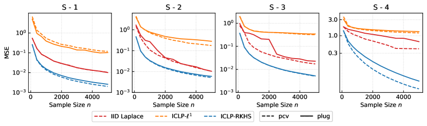
Figure 1: MSE for plug-in and PCV approaches to select regularization parameter $\psi$ under different mechanisms, sample size and true mean functions. The values reported are averages over $100$ independent repetitions. One standard error is on the order of graph line width.

In Figure 1, we report the MSE for each mechanism for different sample size $n$ with $\epsilon=1$. For the rather simple $\mu_{0}$ in S-1, the MSE curves of the plug-in almost line up with the PCV ones for IID Laplace, $\ell^{1}$, and RKHS regularization. In S-2 and S-3, the ICLP mechanism still has consistent curves between the plug-in and PCV while the plug-in MSE curve of the IID Laplace has a step-down pattern. This pattern is due to the fact that the maximum number in $\mathcal{M}$ is determined by the sample size, so with complex curves and small sample sizes, the IID Laplace does not have enough components to estimate the mean of the curve well, but as the sample size increases, more available components make the estimate better. In S-4, PCV does better than the plug-in approach for all mechanisms, which is expected since more components are required in IID Laplace and less penalty is required in RKHS regularization and PCV always did so. Since it has been shown that selecting regularization parameters via the plug-in approach has a reasonable and consistent performance to PCV, we use the plug-in approach in the following simulations to be fully privacy safe.

6.1.2 Comparison of Different Mechanisms

Under the same settings, we compare the performance of different mechanisms under different sample sizes $n$ via MSE. The results are reported in Figure 2.

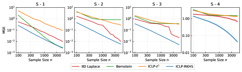
Figure 2: MSE for different mechanisms under different sample sizes $n$ and true mean functions. The values reported are averages over $100$ independent repetitions. One standard error is on the order of graph line width.

It is known that the optimal non-private MSE under $L^{2}$ norm is of order $n^{-1}$, and it should be a straight line with slope $-1$ after taking $\log_{10}$. From Figure 2, it can be observed that the ICLP mechanism with the RKHS regularization approach always achieves the best performance under all scenarios. Its MSE curves also decrease in the same pattern as the desired optimal non-private MSE in S-1 to S-3 while in S-4, the MSE decreases slower than expected with small $n$ as the plug-in value will over smooth summaries, but return parallel with the straight line as n increases. On the other hand, the $\ell^{1}$ regularization is almost the worse one as expected. The IID Laplace and Bernstein are quite close to the RKHS regularization in S-1, showing their effectiveness in simpler curve scenarios, but they fail to mimic the behaviors of the RKHS regularization where curves’ shapes are more complex i.e. S-2 to S-4. Although the IID Laplace can narrow the gap from the RKHS regularization, this only happens as $n$ increases, and thus its effectiveness can be restrictive when limited samples are available.

6.2 Simulation for Density Kernel Estimator Protection

To demonstrate the wide range of application scenarios of the ICLP mechanism, we conduct a simulation on private kernel density estimates. We consider the setting under $\mathbb{R}$ and $\mathbb{R}^{2}$ with samples generated from two mixture Gaussian distributions.

1. $\mathbb{R}$ setting:

   $$x_{i}\stackrel{{\scriptstyle i.i.d.}}{{\sim}}\sum_{i=1}^{2}p_{i}\mathcal{N}(\mu_{i},0.1;0,1),$$

   where $\mathcal{N}(\mu,\sigma;a,b)$ is a truncated normal distribution over $[a,b]$ and $p_{1}=0.6$, $\mu_{1}=0.3$, $\mu_{2}=0.7$.

2. $\mathbb{R}^{2}$ setting:

   $$\mathbf{x}_{i}\stackrel{{\scriptstyle i.i.d.}}{{\sim}}\sum_{i=1}^{2}p_{i}\mathcal{N}\left(\mu_{i},\big{(}\begin{smallmatrix}1&0.5\\ 0.5&1\end{smallmatrix}\big{)};\big{(}\begin{smallmatrix}5\\ -5\end{smallmatrix}\big{)},\big{(}\begin{smallmatrix}5\\ -5\end{smallmatrix}\big{)}\right)$$

   where $\mathcal{N}(\mu,\Sigma;\mathbf{a},\mathbf{b})$ is a multivariate truncated normal distribution over $[a_{1},b_{1}]\times[a_{2},b_{2}]$. Specifically, we take $p_{1}=0.6$, $\mu_{1}=(-3,-3)$, $\mu_{2}=(3,2)$.

We compare the ICLP mechanism (RKHS regularization), IID Laplace, and the Bernstein mechanism. For the ICLP mechanism and the Bernstein mechanism, we pick multiple smoothing parameters $\eta$ and lattice number $K$ to demonstrate how they affect private curves and surfaces; while for IID Laplace, we select the truncated number that provides the best fit under PCV criteria. We generate $2000$ samples under each scenario and use the Gaussian kernel in $\mathbb{R}$ and exponential kernel in $\mathbb{R}^{2}$. We use $h\asymp n^{1/(4+d)}$ where $d=1,2$ to ensure we gain privacy for free and being privacy safe. The results are reported in Figure 3 and Figure 4.

First, for the univariate setting, we can see the ICLP mechanism performs similarly to the IID Laplace; a higher $\eta$ produces less variability in the curves but tends to be over-smooth. The Bernstein mechanism needs over $30$ lattice points in the interval to catch the shape of the bimodal curve but results in producing a messy tail at both ends. A lower lattice number produces better tails but fails to catch the bimodal pattern.

(a)

(b)

(c)

(d)

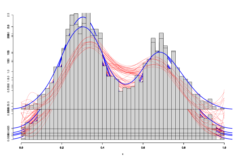
(e)

(f)

Figure 3: Non-private (Blue) and 10 random realization of private (Red) KDE curves. (a) ICLP mechanism with $\eta=1.25$ (b) ICLP mechanism with $\eta=1.5$ (c) IID Laplace and (d)-(f) Bernstein mechanism with $K=10,30,50$.

(a)

(b)

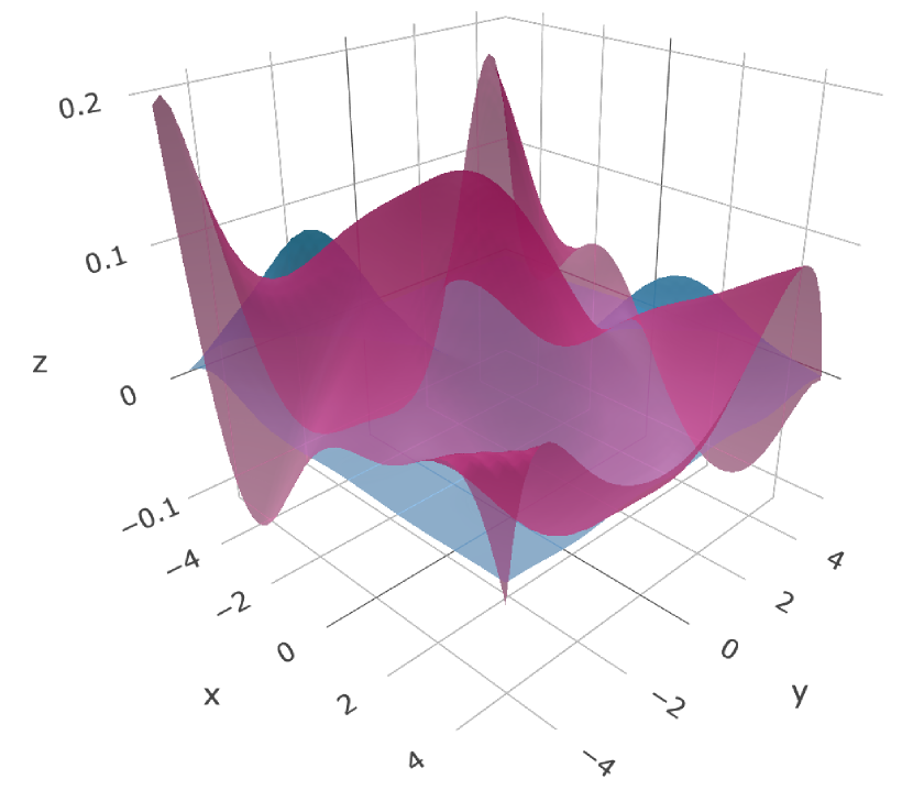
(c)

(d)

(e)

(f)

Figure 4: 3D plot of non-private (Blue) and private (Red) KDE over $\mathbb{R}^{2}$. (a)-(c) ICLP mechanism with $\eta=1.01,1.05,1.2$ (d) IID Laplace and (e)-(f) Bernstein mechanism with $K=5,10$.

For $\mathbb{R}^{2}$ we can see by slightly over smoothing, the ICLP mechanism releases private KDEs very close to non-private ones. A smaller $\eta$ (Figure 4(a)) is more precise at peaks but will be ”noisy” around lower density regions; while a larger $\eta$ (Figure 4(c)) produces smooth lower density regions but causes underestimating at peaks. Figure 4(b) shows that there is a clear ”sweet point” to tradeoff smoothness and underestimation. The IID Laplace performs similarly to the underestimating ICLP case, but the peaks of private KDE don’t fully line up with the non-private one. The Bernstein mechanism, on the other hand, fails to produce similar surfaces to the non-private estimator even though we increase the number of lattice points.

7 Real Applications

This section presents two real data applications of the proposed methods to study releasing functional summaries for different types of functional datasets.

7.1 Application to Medical and Energy Usage Data

In this section, we aim to release a private mean function that satisfies $\epsilon$-DP for the following two different type datasets: First, we consider medical data of Brain scans Diffusion Tensor Imaging (DTI) dataset available in the r package refund. The DTI dataset provides fractional anisotropy (FA) tract profiles for the corpus callosum (CCA) of the right corticospinal tract (RCST) for patients with Multiple Sclerosis and for controls. Specifically, we study the CCA data, with 382 patients measured at 93 equally spaced locations of the CCA. Second, we study the Electricity demand in the Adelaide dataset available in the r package fds. The dataset consists of half-hourly electricity demands from Sunday to Saturday in Adelaide between 6/7/1997 and 31/3/2007. Our analysis focuses on Monday specifically, meaning the dataset consists of 508 days measured at 48 equally spaced time points. Producing privacy-enhanced versions of summaries for such type of energy data is meaningful for protecting public energy institutions such as the power grid from hackers’ attacks.

To measure the performance of each mechanism, since the true mean function is not available under such settings, we use the expected distance between the release summary, $\tilde{\mu}$, and the non-private sample means, $\hat{\mu}$, i.e. $\operatorname{E}\|\tilde{\mu}-\hat{\mu}\|_{L^{2}}^{2}$. We consider Matérn kernel with $\alpha=1.5$ and $2.5$ and $\rho=0.1$. The expectation is approximated by Monte-Carlo with $1000$ generated $\tilde{\mu}$. The results are reported in Table 2 and each data point is an average of $100$ replicate experiments. We also visualized private mean estimates for each mechanism in Figure 5. From Figure 2, it can be observed that the expected distance decreases in a similar pattern as the privacy budget increases for both data sets. We can see that the expected distance of the IID Laplace soon stops changing, which shows that most of the errors of the IID Laplace are concentrated on statistical errors. This shows that in order to avoid adding too much noise to the later components, the IID Laplace has to compromise on using fewer leading components, which leads to higher statistical errors. This can also be seen in Figure 5, where the IID Laplace (green one) can only estimate an approximate shape, but fail to get a better shape estimate locally. $\ell^{1}$ regularization and Bernstein mechanism also have similar performance patterns and have much worse results for smaller budgets. Finally, the RKHS regularization performs the best among all approaches as its released summaries (blue ones) can estimate the shapes precisely and also have much smaller expected distances than the non-private mean.

		Eletricity Demand
Kernel	$\epsilon$	I.I.D. Laplace	Bernstein	$\ell^{1}$	RKHS
$C_{\frac{3}{2}}$	1/8	$0.2828_{0.1981}$	$2.2110_{1.5374}$	$3.9110_{2.9464}$	$1.3726_{1.2935}$
	1/4	$0.1731_{0.0419}$	$0.6140_{0.3859}$	$1.0391_{0.8066}$	$0.3459_{0.2783}$
	1/2	$0.1453_{0.0098}$	$0.2117_{0.1276}$	$0.3415_{0.1897}$	$0.0895_{0.0686}$
	1	$0.1383_{0.0025}$	$0.1106_{0.0352}$	$0.1649_{0.0728}$	$0.0241_{0.0171}$
	2	$0.1366_{0.0007}$	$0.0858_{0.0151}$	$0.1204_{0.0238}$	$0.0080_{0.0044}$
	4	$0.1362_{0.0002}$	$0.0793_{0.0074}$	$0.1089_{0.0105}$	$0.0039_{0.0011}$
$C_{\frac{5}{2}}$	1/8	$0.2805_{0.1645}$	$2.2279_{1.5880}$	$4.1614_{3.5764}$	$1.4261_{1.3547}$
	1/4	$0.1703_{0.0376}$	$0.6053_{0.4227}$	$1.1168_{0.8931}$	$0.3468_{0.2963}$
	1/2	$0.1427_{0.0094}$	$0.2092_{0.0954}$	$0.3497_{0.2276}$	$0.0920_{0.0692}$
	1	$0.1360_{0.0026}$	$0.1109_{0.0374}$	$0.1639_{0.0655}$	$0.0251_{0.0168}$
	2	$0.1342_{0.0006}$	$0.0857_{0.0167}$	$0.1164_{0.0233}$	$0.0089_{0.0049}$
	4	$0.1338_{0.0002}$	$0.0794_{0.0072}$	$0.1044_{0.0090}$	$0.0048_{0.0012}$
		DTI(cca)
Kernel	$\epsilon$	I.I.D. Laplace	Bernstein	$\ell^{1}$	RKHS
$C_{\frac{3}{2}}$	1/8	$0.6305_{0.2878}$	$6.2473_{4.2907}$	$4.4245_{3.9617}$	$3.1996_{2.6794}$
	1/4	$0.4418_{0.0663}$	$1.6122_{1.0886}$	$1.2691_{1.1059}$	$0.8039_{0.6994}$
	1/2	$0.3952_{0.0165}$	$0.4929_{0.3046}$	$0.4701_{0.2522}$	$0.2040_{0.1627}$
	1	$0.3836_{0.0045}$	$0.2080_{0.0824}$	$0.2747_{0.0756}$	$0.0555_{0.0369}$
	2	$0.3809_{0.0010}$	$0.1361_{0.0285}$	$0.2265_{0.0265}$	$0.0186_{0.0106}$
	4	$0.3801_{0.0003}$	$0.1187_{0.0133}$	$0.2143_{0.0133}$	$0.0094_{0.0028}$
$C_{\frac{5}{2}}$	1/8	$0.6303_{0.2867}$	$6.2155_{4.8556}$	$4.7453_{4.0892}$	$3.0841_{2.7095}$
	1/4	$0.4437_{0.0762}$	$1.6275_{1.1514}$	$1.3049_{0.9318}$	$0.7820_{0.7225}$
	1/2	$0.3974_{0.0158}$	$0.4907_{0.3274}$	$0.4793_{0.2431}$	$0.2028_{0.1790}$
	1	$0.3859_{0.0040}$	$0.2073_{0.0890}$	$0.2748_{0.0804}$	$0.0581_{0.0395}$
	2	$0.3830_{0.0010}$	$0.1366_{0.0287}$	$0.2231_{0.0325}$	$0.0216_{0.0107}$
	4	$0.3823_{0.0003}$	$0.1187_{0.0137}$	$0.2102_{0.0126}$	$0.0126_{0.0029}$

Table 2: Expected distance between release mean function estimate and sample mean for Electricity demand and DTI(cca) data sets. The numbers in the subscript indicate the standard error ($\times 10^{-3}$).

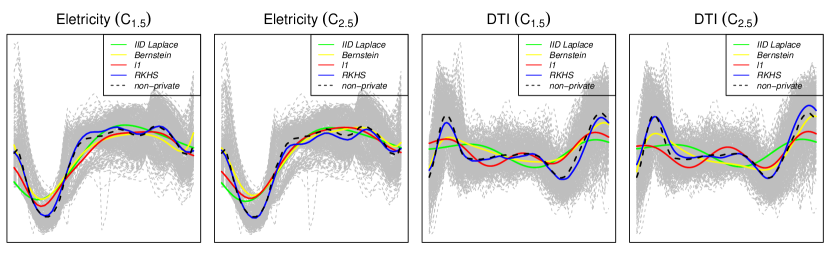
Figure 5: Non-private sample mean and private means for different mechanisms with Matérn kernel $C_{\frac{3}{2}}$ and $C_{\frac{5}{2}}$ with $\epsilon=1$. The curves in light grey indicate the original samples.

7.2 Application to Human Mortality Data

Publishing the entire age-at-death distribution in a given country/region usually provides more comprehensive information about human lifespan and health status than publishing crude mortality rates, and a privacy-enhanced version of this distributional type summary ensures that an attacker cannot infer information about individuals/groups in a particular age range. Following, we study how to release privacy-safe mortality distributions across different regions. The mortality data for each region are collected from the United Nation World Population Prospects 2019 Databases (https://population.un.org/wpp/Download), and the data table record the number of deaths for each region and age.

We estimate the probability density function for each region and private the estimates via the proposed method and its competitors. The privacy budget is set to be $1$. Again, we measure the performance between via $\operatorname{E}\|\tilde{f}-\hat{f}\|_{L^{2}}^{2}$ where $\tilde{f}$ is the private KDE and $\hat{f}$ is non-private one, and the expectation is approximated via Monte Carlo by $200$ private KDEs. The results are reported in Table 3. Again, we visualized the private KDEs for each region and mechanism in Appendix B. From the table, we see the ICLP mechanism (RKHS approach) with $\eta=1.01$ has smaller errors in developing regions while IID Laplace is better in developed regions. This is reasonable as developed regions usually have better medical conditions so that the mortality age concentrates between $70$ and $80$ and their densities are unimodal, and thus a few leading components/basis are sufficient to represent the density function in these regions. Under this scenario, it is understandable that the IID Laplace is better since the noise needed are added to a few components. On the other hand, the situations are opposite in developing regions, where the infant mortality rates are higher. Therefore, these density functions show a multi-modal pattern and require more components/basis to get a close approximation, and the ICLP mechanism assigns less randomness to the summaries thanks to its heterogeneous variance noise injection procedure.

	Mechanisms
Region	RKHS ($\eta=1.01$)	RKHS ($\eta=1.05$)	I.I.D. Laplace	Bernstein ($K=10$)	Bernstein ($K=20$)
Eastern Africa	$\textbf{1.685}_{10.507}$	$5.249_{7.549}$	$5.252_{7.881}$	$3.823_{12.243}$	$2.400_{11.896}$
Middle Africa	$\textbf{1.122}_{0.451}$	$5.281_{0.410}$	$4.870_{2.152}$	$3.969_{0.313}$	$2.090_{0.327}$
Northern Africa	$\textbf{2.398}_{0.680}$	$8.873_{0.656}$	$3.991_{1.807}$	$11.315_{0.546}$	$5.710_{0.646}$
Southern Africa	$2.487_{1.491}$	$6.427_{0.919}$	$2.990_{1.809}$	$3.964_{0.666}$	$\textbf{2.395}_{0.763}$
Western Africa	$\textbf{1.588}_{13.699}$	$5.775_{9.216}$	$5.752_{11.482}$	$4.347_{15.649}$	$2.609_{15.493}$
Central Asia	$\textbf{5.804}_{2.715}$	$11.829_{1.547}$	$7.319_{3.739}$	$13.163_{1.346}$	$8.116_{1.808}$
Eastern Asia	$\textbf{3.551}_{4.414}$	$13.446_{6.872}$	$3.900_{6.958}$	$15.878_{14.110}$	$8.162_{9.175}$
Southern Asia	$\textbf{2.040}_{2.267}$	$8.619_{3.737}$	$2.968_{2.962}$	$10.044_{8.099}$	$4.962_{4.888}$
South-Eastern Asia	$\textbf{2.259}_{1.871}$	$9.498_{3.565}$	$2.566_{2.323}$	$10.428_{8.328}$	$5.157_{4.778}$
Western Asia	$\textbf{2.195}_{0.585}$	$8.689_{0.624}$	$3.768_{2.005}$	$9.380_{0.510}$	$4.640_{0.578}$
Eastern Europe	$\textbf{3.990}_{3.658}$	$13.501_{4.924}$	$4.817_{5.762}$	$15.542_{9.356}$	$8.438_{6.414}$
Northern Europe	$7.318_{1.626}$	$19.087_{1.187}$	$\textbf{7.174}_{1.493}$	$22.846_{1.218}$	$13.339_{1.304}$
Southern Europe	$7.457_{0.977}$	$21.076_{0.931}$	$\textbf{7.137}_{1.083}$	$27.500_{0.852}$	$15.873_{0.927}$
Western Europe	$6.819_{2.184}$	$19.959_{2.782}$	$\textbf{6.445}_{3.417}$	$25.606_{5.375}$	$14.760_{3.965}$
Caribbean	$6.453_{2.890}$	$11.247_{2.022}$	$\textbf{5.981}_{3.634}$	$10.714_{1.580}$	$7.231_{2.296}$
Central America	$1.636_{0.548}$	$7.777_{0.685}$	$\textbf{1.146}_{0.537}$	$5.637_{0.480}$	$2.616_{0.448}$
South America	$\textbf{2.244}_{2.498}$	$9.461_{4.096}$	$2.886_{3.276}$	$9.294_{6.744}$	$4.700_{4.333}$
Northern America	$2.205_{1.734}$	$10.605_{2.792}$	$\textbf{1.537}_{2.297}$	$10.028_{5.546}$	$4.746_{3.153}$
Australia/New Zealand	$23.525_{11.299}$	$29.495_{5.040}$	$\textbf{22.782}_{8.189}$	$28.339_{5.053}$	$23.983_{7.582}$

Table 3: Expected $L^{2}$ distance between release KDEs and non-private KDEs for each region with $\epsilon=1$. The numbers in the subscript indicate the standard error ($\times 10^{-3}$).

8 Conclusion

In this paper, we proposed a new mechanism, the ICLP mechanism, to achieve $\epsilon$-DP for infinite-dimensional objects. It provides a wide range of output privacy protections with more flexible data assumptions and a more robust noise injection process than current mechanisms. Theorem 6 and 8 establish its feasibility in separable Hilbert spaces and spaces of continuous functions. Several approaches are proposed to construct qualified summaries compatible with the ICLP mechanism., along with plug-in parameters selection to guarantee end-to-end protection. In the example of mean function privacy protection, we also show that slightly over-smoothing the summary promotes the trade-off between utility and privacy, and can match the known optimal rate for mean function estimation.

There are some limitations of the proposed mechanism and interesting future works. As we show in Section 5, the implementation of the ICLP mechanism relies on the Karhunen-Loéve expansion and thus will be computationally expensive. Therefore, a computation approach that doesn’t rely on the Karhunen-Loéve expansion is an important future direction. Additionally, even though various experiment results show that by appropriately processing the sample trajectories and the ICLP covariance kernel, omitting the constant for plug-in values has led to satisfactory performance, we believe a more careful investigation of the constant can further enhance performance.

Acknowledgments and Disclosure of Funding

This work was partially supported by the National Science Foundation, NSF SES-1853209.

Appendix A Appendix: Main Proofs

A.1 Proof of Lemma 5

Proof  To show the explicit form of Randon-Nikodym derivative of $P_{D}$ w.r.t. $P_{0}$, we define an isometry between $\mathbb{H}$ and $l^{2}$ to avoid considering probability measures over $\mathbb{H}$. Given an orthonormal basis $\{\phi_{j}\}_{j=1}^{\infty}$ of $\mathbb{H}$, one can define a mapping $\mathcal{T}:\mathbb{H}\rightarrow l_{2}$ by $\mathcal{T}(f)=\{\langle f,\phi_{j}\rangle\}_{j=1}^{\infty}$, and its inverse is $\mathcal{T}^{-1}(\{\langle f,\phi_{j}\rangle\})=\sum_{j=1}^{\infty}\langle f,\phi_{j}\rangle\phi_{j}$. This mapping is an isometry between $\mathbb{H}$ and $l^{2}$ and we can consider the probability measure over $l^{2}$ rather than over $\mathbb{H}$.

For a Laplace r.v.s. $X\sim\operatorname{Lap}(\mu,b)$ over $\mathbb{R}$, it induces a probability measure over $(\mathbb{R},\mathcal{B})$, where $\mathcal{B}$ is the borel set over $\mathbb{R}$, as

$$\gamma_{\mu,b}(dx)=\frac{1}{2b}exp\left(-\frac{|x-\mu|}{b}\right)dx.$$

Let $\{(\lambda_{j},\phi_{j})\}_{j\in\mathbb{N}}$ be the eigencomponents (eigenfunctions and eigenvalues) of $C$ and let $\lambda_{j}=2b_{j}^{2}$. By Existence of Product Measures Theorem (Tao, 2011) and isomorphism mapping $\mathcal{T}$, $P_{D}\circ\mathcal{T}$ is a unique probability measure defined as $\gamma(f_{D},C):=\prod_{j=1}^{\infty}\gamma_{f_{Dj},b_{j}}$ over $(\mathbb{R}^{\infty},\mathcal{B}^{\infty}):=(\prod_{j=1}^{\infty}\mathbb{R}_{j},\prod_{j=1}^{\infty}\mathcal{B}_{j})$. We further restrict $\gamma(f_{D},C)$ on $(l^{2},\sigma(l^{2}))$ and keep denoting it by $\gamma(f_{D},C)$. We now start to prove Lemma $1$, by showing the form of Radom-Nikodym derivative of $\gamma(h,C)$ w.r.t. $\gamma(0,C)$ is the same as derivative of $\{P_{D}:D\in\mathcal{D}\}$ to $P_{0}$ and takes the form of

$$\frac{dP_{h}}{dP_{0}}(z)=exp\left\{-\frac{1}{\sigma}\left(\left\|z-h\right\|_{1,C}-\left\|z\right\|_{1,C}\right)\right\},$$ (12)

First, we need to show the r.h.s. of the above Equation is well-defined when $h\in\mathcal{H}_{C}$. Define

$$H_{M}(z)=\sum_{j=1}^{M}\frac{|z_{j}-h_{j}|-|z_{j}|}{b_{j}}\quad\textit{and}\quad H(z)=\lim_{M\rightarrow\infty}H_{M}(z).$$

We need to show there exists a set $A$ with $P_{0}(A)=1$ such that $H(z)$ exists and is finite on $A$. Suppose $z_{j}\sim\operatorname{Lap}(0,b_{j})$, with some calculation, one has

$$\operatorname{Var}\left(H_{M}(z)\right) =\sum_{j=1}^{M}\operatorname{Var}\left(\frac{|z_{j}-h_{j}|-|z_{j}|}{b_{j}}\right)$$

$$=\sum_{j=1}^{M}\left(1-\exp\left\{-\frac{h_{j}}{b_{j}}\right\}\right)$$

$$=\sum_{j=1}^{M}\frac{h_{j}^{2}}{b_{j}^{2}},$$

where the last equality is by Taylor expansion. By Fatou’s Lemma and condition $h\in\mathcal{H}_{C}$, $\operatorname{Var}(H(z))<\infty$. The set $A$ is $\Omega$ and therefore with $P_{0}$-measure 1. Therefore, once $h\in\mathcal{H}_{C}$, then r.h.s. of Equation exists and is well-defined.

Next, we aim to prove that $\frac{dP_{h}}{dP_{0}}(z)$ is the Radon-Nikodym derivative of $h+\sigma Z$ w.r.t. $\sigma Z$. Let $g(x)=exp\left\{-\frac{\sqrt{2}}{\sigma}\left(\left\|x-h\right\|_{1,C}-\left\|x\right\|_{1,C}\right)\right\}$ and $dP_{h}^{*}(x)=g(x)dP_{0}(x)$. Therefore, we only need to show that $P_{h}$ and $P_{h}^{*}$ are the same measure. We finish this proof by showing they have the same moment generating function.

$$MGF_{P_{h}}(t) =\operatorname{E}_{P_{h}}exp\left\{\langle X,t\rangle_{\mathbb{H}}\right\}$$

$$=\prod_{j=1}^{\infty}\int_{\mathbb{R}}exp\left\{x_{j}t_{j}\right\}d\gamma_{h_{j},b_{j}}(x_{j})$$

$$=\prod_{j=1}^{\infty}\frac{exp\left\{h_{j}t_{j}\right\}}{1-(b_{j}t_{j})^{2}}.$$

where the second inequality comes from the result that $P_{h}$ is product measure of $\gamma_{h_{j},b_{j}}$. For the moment generate function of $P_{h}^{*}$,

$$MGF_{P_{h}^{*}}(t) =\operatorname{E}_{P_{h}^{*}}exp\left\{\langle X,t\rangle_{\mathbb{H}}\right\}$$

$$=\operatorname{E}_{Q}g(X)exp\left\{\langle X,t\rangle_{\mathbb{H}}\right\}$$

$$=\prod_{j=1}^{\infty}\int_{\mathbb{R}}exp\left\{-\frac{1}{\sigma}\left(\frac{|x_{j}-h_{j}|-|x_{j}|}{b_{j}}\right)+x_{j}t_{j}\right\}d\gamma_{0,b_{j}}(x_{j})$$

$$=\prod_{j=1}^{\infty}\int_{\mathbb{R}}exp\left\{x_{j}t_{j}\right\}d\gamma_{h_{j},b_{j}}(x_{j})$$

$$=\prod_{j=1}^{\infty}\frac{exp\left\{h_{j}t_{j}\right\}}{1-(b_{j}t_{j})^{2}}=MGF_{P_{h}}(h).$$

Therefore, $P_{h}$ and $P_{h}^{*}$ are the same measures.  

A.2 Proof of Theorem 3

Proof  To prove the existence of the ICLP in $\mathbb{H}$, we only need to prove $\operatorname{E}\langle X,X\rangle_{\mathbb{H}}<\infty$, then the proof can be done by Fubini’s theorem. Notice

$$\operatorname{E}\langle X,X\rangle_{\mathbb{H}}=\operatorname{E}\sum_{j\geq 1}\sum_{k\geq 1}\sqrt{\lambda_{j}}\sqrt{\lambda_{k}}Z_{j}Z_{k}\langle\phi_{j},\phi_{k}\rangle_{\mathbb{H}}=\operatorname{E}\sum_{j=1}^{\infty}\lambda_{j}Z_{j}^{2}$$

Since $\sum_{j=1}^{\infty}\operatorname{E}\lambda_{j}Z_{j}^{2}=\sum_{j=1}^{\infty}\lambda_{j}<\infty$, by Fubini’s theorem, $\operatorname{E}\langle X,X\rangle_{\mathbb{H}}<\infty$, which proves the existence of $X$.  

A.3 Proof of Theorem 4

Proof  By the fact that $\mathcal{T}$ is an isomorphism mapping between $\mathcal{H}$ and $l^{2}$, to prove $P_{D}$ and $P_{D^{\prime}}$ are equivalent, it’s sufficient to prove $\gamma(f_{D},C)$ and $\gamma(f_{D^{\prime}},C)$ are equivalent.

We now formally prove $\gamma(h,C)$ and $\gamma(0,C)$ iff $h\in\mathcal{H}_{C}$. For “if” part, for two infinite product measures, we can apply Kakutani’s theorem (Kakutani, 1948). Then the two measure are equivalent if

$$\sum_{j=1}^{\infty}\log\int_{R}\sqrt{\frac{\gamma_{j}(h_{j},b_{j})}{\gamma_{j}(0,b_{j})}}\gamma_{j}(0,b_{j})(dx).$$

A few calculation leads to the target space is

$$\mathcal{H}_{C}^{*}=\left\{h\in\mathbb{H}:\sum_{j\geq 1}\left[\frac{|h_{j}|}{2b_{j}}-log(1+\frac{|h_{j}|}{2b_{j}})\right]<\infty\right\},$$

and we now prove that, $\mathcal{H}_{C}^{*}=\mathcal{H}_{C}$. We only need to prove that for a non-negative sequence $\{a_{j}\}_{j\geq 1}$, the series $\sum_{j\geq 1}[a_{n}-log(1+a_{n})]$ converges if and only if $\sum_{j\geq 1}a_{n}^{2}$ converges. Let $f(x)$ be the Taylor expansion of $x-log(1+x)$ and $g(x)=x^{2}$. Besides, note that $\lim_{n\rightarrow\infty}f(a_{n})=0$ if and only if $\lim_{n\rightarrow\infty}a_{n}=0$. Thus,

• If $\sum_{j\geq 1}[a_{n}-log(1+a_{n})]<\infty$, then $\lim_{n\rightarrow\infty}f(a_{n})=0$ and so $\lim_{n\rightarrow\infty}a_{n}=0$. Then,

  $$\lim_{n\rightarrow\infty}\frac{f(a_{n})}{g(a_{n})}=\lim_{n\rightarrow\infty}\frac{a_{n}-log(1+a_{n})}{a_{n}^{2}}=\frac{1}{2}$$

  therefore by limit comparison test $\sum_{j\geq 1}a_{n}^{2}$ converges too.

• If $\sum_{j\geq 1}a_{n}^{2}<\infty$, by the same statement as above also holds and therefore $\sum_{j\geq 1}[a_{n}-log(1+a_{n})]<\infty$.

For the “only if” part, the argument is the same as proof of Theorem 2 in Reimherr and Awan (2019).  

A.4 Proof of Theorem 6

Proof  We prove the theorem via contradiction. Assume if $f_{D}\in\mathcal{H}_{C}\backslash\mathcal{H}_{1,C}$, for any given fixed $\epsilon$, $\exists\ \sigma\in\mathbb{R}$ such that mechanism $f_{D}+\sigma Z$ still satisfy $\epsilon$-DP, then by post-process property of differential privacy, we know that for any transformation $G:\mathcal{H}\rightarrow\mathcal{H}$, $G(f_{D})$ is also $\epsilon$-DP. Now, $\forall\ J\in\mathbb{N}$, consider $G$ to be a projection mapping into first $J$ components, i.e. $G_{J}(f_{D})=\sum_{j=1}^{J}\langle f_{D},\phi_{j}\rangle\phi_{j}$. Therefore, by assumption, $\forall\ J\in\mathbb{N}$, $G_{J}(f_{D})$ is $\epsilon$-DP, i.e.

$$exp\left\{-\frac{\sqrt{2}}{\sigma}\sum_{j=1}^{J}\left(\frac{|\langle f_{D}-z,\phi_{j}\rangle|}{\sqrt{2}b_{j}}-\frac{|\langle z,\phi_{j}\rangle|}{\sqrt{2}b_{j}}\right)\right\}\leq exp\left\{\epsilon\right\},$$

except for $z\in A$ where $A$ is zero-measure set.

Define $B_{j}=\left\{z_{j}:\left|z_{j}\right|>\left|f_{j}\right|\right\}$ and $S_{J}=\left\{z\in l^{2}:z_{j}\in B_{j},\forall 1\leq j\leq J\ \textit{and}\ z_{j}\in\mathbb{R},\forall j>J\right\}$. Then $\forall\ z\in S_{J}$,

$$exp\left\{-\frac{\sqrt{2}}{\sigma}\sum_{j=1}^{J}\left(\frac{|\langle f_{D}-z,\phi_{j}\rangle|}{\sqrt{2}b_{j}}-\frac{|\langle z,\phi_{j}\rangle|}{\sqrt{2}b_{j}}\right)\right\}=exp\left\{\frac{\sqrt{2}}{\sigma}\sum_{j=1}^{J}\left(\frac{|\langle f_{D},\phi_{j}\rangle|}{\sqrt{2}b_{j}}\right)\right\}\leq exp\left\{\epsilon\right\}.$$

However, since $h\in\mathcal{H}_{K}\backslash\mathcal{H}_{1,C}$, one can always find an $J$ s.t. $exp\left\{\frac{1}{\sigma}\sum_{j=1}^{J}\frac{|\langle f_{D},\phi_{j}\rangle|}{b_{j}}\right\}>exp\left\{\epsilon\right\}$ and therefore contradiction holds and no such $\sigma\in\mathbb{R}^{+}$ exists.

The remaining thing will be to prove $S_{J}$ is not a zero-measure set. By Existence of Product Measure in Tao (2011),

$$\gamma_{0,C}(S_{J})=\prod_{j=1}^{J}\gamma_{0,\sqrt{2}b_{j}}(B_{j})$$

where r.h.s. greater than $0$ by definition of $B_{j}$.  

A.5 Proof of Theorem 7

Proof  By Lemma $1$, the density of $\tilde{f}_{D}$ w.r.t. to $\sigma Z$ is

$$\frac{dP_{D}}{dP_{0}}(z)=exp\left\{-\frac{1}{\sigma}\left(\left\|z-f_{D}\right\|_{1,C}-\left\|z\right\|_{1,C}\right)\right\}.$$

We aim to show that for any measurable subset $A\subseteq\mathbb{H}$, one has

$$P_{D}(A)\leq e^{\epsilon}P_{D^{\prime}}(A),$$

which is equivalent to show

$$P_{D}(A)=\int_{A}dP_{D}(x)=\int_{A}\frac{dP_{D}}{dP_{D^{\prime}}}(x)dP_{D^{\prime}}(x)\leq e^{\epsilon}\int_{A}dP_{D^{\prime}}(x).$$

Then

$$\frac{dP_{D}}{dP_{D^{\prime}}}(x) =\frac{dP_{D}}{dP_{0}}(x)/\frac{dP_{D^{\prime}}}{dP_{0}}(x)$$

$$=exp\left\{-\frac{1}{\sigma}\left(\left\|x-f_{D}\right\|_{1,C}-\left\|x-f_{D^{\prime}}\right\|_{1,C}\right)\right\}$$

$$\leq exp\left\{\frac{1}{\sigma}\left\|f_{D^{\prime}}-f_{D}\right\|_{1,C}\right\}.$$

Recall the global sensitivity for the ICLP mechanism is

$$\Delta=\sup_{D\sim D^{\prime}}\|f_{D}-f_{D^{\prime}}\|_{1,C},$$

therefore, $\forall x\in\mathbb{H}$, $\frac{dP_{D}}{dP_{D^{\prime}}}(x)\leq e^{\epsilon}$ and

$$P_{D}(A)=\int_{A}\frac{dP_{D}}{dP_{D^{\prime}}}(x)dP_{D^{\prime}}(x)\leq e^{\epsilon}\int_{A}dP_{D^{\prime}}(x)$$

holds.  

A.6 Proof of Theorem 8

Proof 

$$Z(t)-Z(s)=\sum\lambda_{j}^{1/2}Z_{j}(\phi_{j}(t)-\phi_{j}(s))$$

So

$$\operatorname{E}[\exp\{t(Z(t)-Z(s))\}] =\prod_{j=1}^{\infty}\frac{1}{1-t^{2}\lambda_{j}(\phi_{j}(t)-\phi_{j}(s))^{2}}$$

$$=\exp\left\{-\sum_{j=1}^{\infty}\log\left(1-\frac{t^{2}\lambda_{j}}{2}(\phi_{j}(t)-\phi_{j}(s))^{2}\right)\right\}$$

with $t$ satisfies

$$0\leq t^{2}\lambda_{j}(\phi_{j}(t)-\phi_{j}(s))^{2}<1,\quad\forall\ j.$$

Notice

$$\lambda_{j}(\phi_{j}(t)-\phi_{j}(s))^{2} =\lambda_{j}\langle C_{t}-C_{s},\phi_{j}\rangle_{C}^{2}$$

$$\leq\langle C_{t}-C_{s},C_{t}-C_{s}\rangle_{C}$$

$$=C(t,t)-2C(t,s)+C(s,s)$$

$$\leq 2M_{C}|t-s|^{\alpha},$$

$M_{C}$ be the Hölder-continuous constant, and this leads to

$$0\leq t\leq(\frac{1}{M_{C}})^{\frac{1}{2}}|t-s|^{-\frac{\alpha}{2}}.$$

Now notice that for $0\leq x<1$ and $f(x)=-\log(1-x)$ we have $f^{\prime}(x)=1/(1-x)$ and so

$$-\log(1-x)=f(x)=f(0)+xf^{\prime}(\zeta)=\frac{x}{1-\zeta}\leq\frac{x}{1-x},$$

for some $\zeta\in(0,x)$. So we have then

$$-\log(1-\frac{t^{2}\lambda_{j}}{2}(\phi_{j}(t)-\phi_{j}(s))^{2}) \leq\frac{\frac{t^{2}\lambda_{j}}{2}(\phi_{j}(t)-\phi_{j}(s))^{2}}{1-\frac{t^{2}\lambda_{j}}{2}(\phi_{j}(t)-\phi_{j}(s))^{2}}$$

$$\leq\frac{t^{2}\lambda_{j}}{2}(\phi_{j}(t)-\phi_{j}(s))^{2}\max_{k}\left\{(1-\frac{t^{2}\lambda_{k}}{2}(\phi_{k}(t)-\phi_{k}(s))^{2})^{-1}\right\}.$$

Again, choose $t$ such that $(1-\frac{t^{2}\lambda_{k}}{2}(\phi_{k}(t)-\phi_{k}(s))^{2})^{-1}\leq M_{0}<\infty$ so that we get

$$\operatorname{E}[\exp\{t(Z(t)-Z(s))\}] \leq\exp\left\{M_{0}\frac{t^{2}}{2}\sum\lambda_{j}(\phi_{j}(t)-\phi_{j}(s))^{2}\right\}$$

$$=\exp\left\{\frac{M_{0}t^{2}}{2}(C(t,t)-2C(t,s)+C(s,s))\right\}$$

$$\leq\exp\left\{M_{0}M_{C}t^{2}|t-s|^{\alpha}\right\}.$$

Therefore, by Chernoff bound, we got

$$P\left(|X(s)-X(t)|\geq a\right) \leq\frac{\operatorname{E}[\exp\{t(Z(t)-Z(s))\}]}{exp\{ta\}}$$

$$\leq exp\left\{M_{0}M_{C}t^{2}|t-s|^{\alpha}-ta\right\}.$$

The minimizer of r.h.s. with respect to $t$ is $t_{0}=\frac{a}{2M_{0}M_{C}|t-s|^{\alpha}}$, with restriction of $t$, we get $a\leq 2M_{0}|t-s|^{\frac{1}{2}\alpha}$.

We consider the following two cases:

Case 1 : Suppose $a\leq 2M_{0}|t-s|^{\frac{1}{2}\alpha}$, then the minimizer is $t_{0}=\frac{a}{2M_{0}M_{C}|t-s|^{\alpha}}$, then

$$P\left(|X(s)-X(t)|\geq a\right)\leq exp\left\{-\tilde{M_{1}}a^{2}|t-s|^{-\alpha}\right\},$$

for some generic constant $\tilde{M}_{1}$ taking $a(x)=C|x|^{\beta}$ with $\beta\geq\frac{1}{2}\alpha$, then

$$\sum_{n=1}^{\infty}a(2^{-n})=\sum_{n=1}^{\infty}2^{-n\beta}\quad\textit{and }\quad\sum_{n=1}^{\infty}2^{n}\exp\{-\tilde{M}_{2}|2^{n}|^{\alpha-2\beta}\},$$

The first series converges if $\beta<1$. However, to make the second one converges, we need $\alpha>2\beta$ which leads to $\alpha>\alpha$, contradiction.

Case 2 : Suppose $a>2M_{0}|t-s|^{\frac{1}{2}\alpha}$, then the minimizer is $t_{0}=(\frac{1}{M_{C}})^{\frac{1}{2}}|t-s|^{-\frac{1}{2}\alpha}$, then

$$r.h.s.=\exp\left\{M_{0}-\left(\frac{1}{M_{C}}\right)^{\frac{1}{2}}|t-s|^{-\frac{1}{2}\alpha}a\right\}.$$

Therefore, for we pick function $a(x)=2M_{0}|x|^{\beta}>2M_{0}|x|^{\frac{1}{2}\alpha}$, with $\beta\in(0,\frac{1}{2}\alpha)$, then $\sum_{j=1}^{\infty}a(2^{-n})<\infty$ and

$$\sum_{j=1}^{\infty}2^{n}b(2^{-n}) =\sum_{j=1}^{\infty}2^{n}\exp\left\{M_{0}-\left(\frac{1}{M_{C}}\right)^{\frac{1}{2}}|2^{-n}|^{-\frac{1}{2}\alpha}a(2^{-n})\right\}$$

$$=\sum_{j=1}^{\infty}2^{n}\exp\left\{M_{0}-\left(\frac{1}{M_{C}}\right)^{\frac{1}{2}}|2^{n}|^{\frac{1}{2}\alpha-\beta}\right\}$$

by the range of $\beta$, we have $\sum_{j=1}^{\infty}2^{n}b(2^{-n})<\infty$. Then the proof is completed by Kolomogorov theorem.  

A.7 Proof of Theorem 9

Proof  To obtain the close form of $\ell^{1}$-regularized estimator, we expand $X_{i}-\theta$ by the eigenfunctions $\phi_{j}$, i.e.

$$\frac{1}{n}\sum_{i=1}^{n}\left\|X_{i}-\theta\right\|^{2}+\psi\|\theta\|_{1,C^{\eta_{l}}} =\frac{1}{n}\sum_{i=1}^{n}\left\|\sum_{j=1}^{\infty}\langle X_{i}-\theta,\phi_{j}\rangle\phi_{j}\right\|^{2}+\psi\|\theta\|_{1,C^{\eta_{l}}}$$ (13)

$$=\frac{1}{n}\sum_{i=1}^{n}\sum_{j=1}^{\infty}\langle X_{i}-\theta,\phi_{j}\rangle^{2}+\psi\|\theta\|_{1,C^{\eta_{l}}}$$

$$=\sum_{j=1}^{\infty}\left\{\frac{1}{n}\sum_{i=1}^{n}(X_{ij}-\theta_{j})^{2}+\psi\frac{|\theta_{j}|}{\lambda_{j}^{\eta_{l}/2}}\right\}$$

Solving the minimization problem with in the bracket, then for each $j$,

$$\hat{\theta}_{j}=\text{sgn}(\bar{X}_{j}-\frac{\psi}{2\lambda_{j}^{\eta_{l}/2}})\left(\bar{X}_{j}-\frac{\psi}{2\lambda_{j}^{\eta_{l}/2}}\right)^{+}.$$

Then

$$\hat{\mu}_{D}^{l}=\sum_{j=1}^{\infty}\hat{\theta}_{j}=\sum_{j=1}^{\infty}s_{\psi,2\lambda_{j}^{\eta_{l}/2}}\left(\left\langle\bar{X},\phi_{j}\right\rangle\right)\phi_{j}.\phi_{j}$$

For the global sensitivity,

$$\sup_{D\sim D^{\prime}}\|\hat{\mu}_{D}^{l}-\hat{\mu}_{D^{\prime}}^{l}\|_{1,C} =\sup_{D\sim D^{\prime}}\sum_{j=1}^{J_{\tau}}\frac{|s_{\psi,\lambda_{j}^{\eta_{l}/2}}\left(\left\langle\bar{X}_{D},\phi_{j}\right\rangle\right)-s_{\psi,\lambda_{j}^{\eta_{l}/2}}\left(\left\langle\bar{X}_{D^{\prime}},\phi_{j}\right\rangle\right)|}{\lambda_{j}^{\frac{\eta_{l}}{2}}}$$

$$\leq\sup_{D\sim D^{\prime}}\sum_{j=1}^{J_{\tau}}\frac{|\left\langle\bar{X}_{D}-\bar{X}_{D^{\prime}},\phi_{j}\right\rangle|}{\lambda_{j}^{\frac{\eta_{l}}{2}}}\leq\frac{2\tau}{n}\sum_{j=1}^{J_{\tau}}\frac{1}{\lambda_{j}^{\frac{\eta_{l}}{2}}},$$

where the first inequality is based on the fact that, in the worst case, the $j$-th coefficients based on $D$ and $D^{\prime}$ will not be shrunk to $0$ simultaneously and thus should have the same sensitivity without soft-threshold function.  

A.8 Proof of Theorem 11

Proof  Recall the object function

$$F(\theta)=\frac{1}{n}\sum_{i=1}^{n}\left\|X_{i}-\theta\right\|^{2}+\psi\|\theta\|_{C^{\eta_{r}}}^{2}.$$

and after dropping everything not involving $\theta$, we have

$$F(\theta) =-2\langle\bar{X},\theta\rangle_{\mathbb{H}}+\langle\theta,\theta\rangle_{\mathbb{H}}+\psi\langle\theta,\theta\rangle_{C^{\eta_{r}}}$$

$$=-2\langle\bar{X},C^{\eta_{r}}\theta\rangle_{C^{\eta_{r}}}+\langle\theta,C^{\eta_{r}}\theta\rangle_{C^{\eta_{r}}}+\psi\langle\theta,\theta\rangle_{C^{\eta_{r}}}.$$

The second equality is based on Hilbert space’s own dual, i.e $\langle\cdot,\cdot\rangle_{\mathbb{H}}=\langle\cdot,C(\cdot)\rangle_{\mathcal{H}_{C}}$. Thus the minimizer of the $F(\theta)$ is

$$\hat{\mu}_{D}^{r} =\left(C^{\eta_{r}}+\psi I\right)^{-1}C^{\eta_{r}}(\bar{X})$$

$$=\sum_{j=1}^{\infty}\frac{\lambda_{j}^{\eta_{r}}}{\lambda_{j}^{\eta_{r}}+\psi}\left\langle\bar{X},\phi_{j}\right\rangle_{\mathbb{H}}\phi_{j}$$

where the second equality follow by expansion $\hat{\mu}_{D}^{r}$ under the eigenfunction $\phi_{j}$. For the global sensitivity, the upper bound for $\sup_{D\sim D^{\prime}}\|\hat{\mu}_{D}^{r}-\hat{\mu}_{D^{\prime}}^{r}\|_{1,C}$ is

$$\sup_{D\sim D^{\prime}}\|\hat{\mu}_{D}-\hat{\mu}_{D^{\prime}}\|_{1,C} =\sup_{D\sim D^{\prime}}\sum_{j=1}^{\infty}\frac{\lambda_{j}^{\eta_{r}-\frac{1}{2}}}{\lambda_{j}^{\eta_{r}}+\psi}\left|\left\langle\bar{X}-\bar{X}^{\prime},\phi_{j}\right\rangle\right|$$

$$\leq\sup_{D\sim D^{\prime}}\sup_{j}\left\{\frac{\lambda_{j}^{\eta_{r}-\frac{1}{2}}}{\lambda_{j}^{\eta_{r}}+\psi}\right\}\sum_{j=1}^{\infty}\left|\left\langle\bar{X}-\bar{X}^{\prime},\phi_{j}\right\rangle\right|$$

$$\leq\sup_{D\sim D^{\prime}}\left\{\frac{1}{n}\sup_{j}\left\{\frac{\lambda_{j}^{\eta_{r}-\frac{1}{2}}}{\lambda_{j}^{\eta_{r}}+\psi}\right\}\sum_{j=1}^{\infty}\left|\left\langle X_{n}-X_{n}^{{}^{\prime}},\phi_{j}\right\rangle\right|\right\}$$

$$\leq\frac{2\tau}{n}\sup_{j}\left\{\frac{\lambda_{j}^{\eta_{r}-\frac{1}{2}}}{\lambda_{j}^{\eta_{r}}+\psi}\right\}.$$

 

A.9 Proof of Theorem 13

Proof  For RKHS regularization:  Recall that the form of $\hat{\mu}_{D}^{r}$ and its global sensitivity, for privacy cost:

$$\operatorname{E}\|\tilde{\mu}-\hat{\mu}\|_{L^{2}}^{2} =\frac{2\Delta^{2}}{\epsilon^{2}}\sum_{j=1}^{\infty}\lambda_{j}$$

$$\lesssim\left(\sup_{j}\frac{\lambda_{j}^{\eta_{r}-\frac{1}{2}}}{\lambda_{j}^{\eta_{r}}+\psi}\right)^{2}\frac{1}{(n\epsilon)^{2}}.$$

Consider $f(x)=\frac{x^{\eta_{r}-0.5}}{x^{\eta_{r}}+\psi}$, and observe that $f(x)\lesssim\psi^{-\frac{1}{2\eta_{r}}}$, then,

$$\operatorname{E}\|\tilde{\mu}-\hat{\mu}\|_{L^{2}}^{2}\lesssim n^{-2}\psi^{-\frac{1}{\eta_{2}}}.$$

For Statistical Error: The $n^{-1}$ part comes from variance while for bias,

$$\|\operatorname{E}\hat{\mu}-\mu_{0}\|_{L^{2}}^{2}=\sum_{j=1}^{\infty}\left(\frac{\psi}{\lambda_{j}^{\eta_{r}}+\psi}\right)^{2}\left\langle\mu_{0},\phi_{j}\right\rangle^{2}\leq\psi\|\mu_{0}\|_{C^{\eta_{r}}}^{2}\lesssim\psi,$$

where the last inequality is by assuming $\|\mu_{0}\|_{C^{\eta_{r}}}<\infty$. Combining privacy cost and statistical error, one get the desired results.

For $\boldsymbol{\ell}^{1}$ regularization: Consider privacy cost, let $J_{\tau}:=\operatorname{max}\{j\geq 1:\tau\leq\psi/2\lambda_{j}^{\eta_{l}/2}\}$, then

$$\operatorname{E}\left\|\tilde{\mu}-\hat{\mu}\right\|_{L^{2}}^{2} =\frac{4\tau^{2}}{n^{2}\epsilon^{2}}\Delta^{2}\sum_{j=1}^{J_{\tau}}\lambda_{j}$$

$$\lesssim\left(\epsilon n\right)^{-2}\left(\sum_{j=1}^{J_{\tau}}j^{\nu}\right)^{2}\sum_{j=1}^{J_{\tau}}j^{-2\nu}$$

$$\lesssim\left(\epsilon n\right)^{-2}J_{\tau}^{\max\{3,2(\nu+1)\}}.$$

As we assume the noise kernel with finite trace, then $\nu>\frac{1}{2}$ and

$$\operatorname{E}\left\|\tilde{\mu}-\hat{\mu}\right\|_{L^{2}}^{2}\lesssim\left(\epsilon n\right)^{-2}J_{\tau}^{2(\nu+1)}.$$

Next, we turn to Statistical Error. Define $\mu_{0,\psi}=\sum_{j=1}^{\infty}f_{\psi,2\lambda_{j}^{\frac{\eta_{l}}{2}}}\left(\left\langle\mu_{0},\phi_{j}\right\rangle\right)\phi_{j}$, by triangular inequality

$$\operatorname{E}\left\|\hat{\mu}-\mu_{0}\right\|_{L^{2}}^{2}\leq\operatorname{E}\left\|\hat{\mu}-\mu_{0,\psi}\right\|_{L^{2}}^{2}+\left\|\mu_{0,\psi}-\mu_{0}\right\|_{L^{2}}^{2}.$$

For the bias term, let $A=\left\{j:|\mu_{j}|\geq\frac{\psi}{2\lambda_{j}^{\eta_{l}/2}}\right\}$, then

$$\left\|\mu_{0,\psi}-\mu_{0}\right\|_{L^{2}}^{2}=\sum_{A}\left(\mu_{0j}-f_{\psi,2\lambda_{j}^{\frac{\eta_{l}}{2}}}(\mu_{0j})\right)^{2}+\sum_{A^{c}}\left(\mu_{0j}-f_{\psi,2\lambda_{j}^{\frac{\eta_{l}}{2}}}(\mu_{0j})\right)^{2}.$$

Starting with the summation over $A$, since $\frac{\lambda_{j}^{-\frac{\eta_{l}}{2}}}{2}<\frac{|\mu_{0j}|}{\psi}$ we have

$$\sum_{A}\left(\mu_{0j}-f_{\psi,2\lambda_{j}^{\frac{\eta_{l}}{2}}}(\mu_{0j})\right)^{2} =\sum_{A}\frac{\psi^{2}}{4\lambda_{j}^{\eta_{l}}}\leq\psi\sum_{A}\frac{\left|\mu_{0j}\right|}{2\lambda_{j}^{\frac{\eta_{l}}{2}}}\leq\frac{\psi}{2}\left\|\mu_{0}\right\|_{1,C^{\eta_{l}}}.$$

Turning to summation over $A^{c}$, since $|\mu_{0j}|\leq\frac{\psi}{2\lambda_{j}^{\frac{\eta_{l}}{2}}}$,

$$\sum_{A^{c}}\left(\mu_{0j}-f_{\psi,2\lambda_{j}^{\frac{\eta_{l}}{2}}}(\mu_{0j})\right)^{2} =\sum_{A^{c}}\mu_{0j}^{2}\leq\psi\sum_{A^{c}}\frac{|\mu_{0j}|}{2\lambda_{j}^{\frac{\eta_{l}}{2}}}\leq\frac{\psi}{2}\left\|\mu_{0}\right\|_{1,C^{\eta_{l}}}.$$

Therefore, the overall bias is bounded by

$$\left\|\mu_{0,\psi}-\mu_{0}\right\|_{L^{2}}^{2}\leq\frac{\psi}{2}\left\|\mu_{0}\right\|_{1,C^{\eta_{l}}}.$$

Now consider variance term $\operatorname{E}\left\|\hat{\mu}-\mu_{0,\psi}\right\|_{L^{2}}^{2}$,

$$\left\|\hat{\mu}-\mu_{0}\right\|_{L^{2}}^{2}=\sum_{j=1}^{\infty}\left(f_{\psi,2\lambda_{j}^{\frac{\eta_{l}}{2}}}\left(\bar{X}_{j}\right)-f_{\psi,2\lambda_{j}^{\frac{\eta_{l}}{2}}}\left(\mu_{0j}\right)\right)^{2}.$$

Similar to bias part, the summation can be decomposed to sum of four disjoint pieces

$$A_{0,0} =\{|\bar{X}_{j}|\leq\psi/2\lambda_{j}^{\frac{\eta_{l}}{2}},|\mu_{j}|\leq\psi/2\lambda_{j}^{\frac{\eta_{l}}{2}}\},$$

$$A_{0,1} =\{|\bar{X}_{j}|\leq\psi/2\lambda_{j}^{\frac{\eta_{l}}{2}},|\mu_{j}|>\psi/2\lambda_{j}^{\frac{\eta_{l}}{2}}\},$$

$$A_{1,0} =\{|\bar{X}_{j}|>\psi/2\lambda_{j}^{\frac{\eta_{l}}{2}},|\mu_{j}|\leq\psi/2\lambda_{j}^{\frac{\eta_{l}}{2}}\},$$

$$A_{1,1} =\{|\bar{X}_{j}|>\psi/2\lambda_{j}^{\frac{\eta_{l}}{2}},|\mu_{j}|>\psi/2\lambda_{j}^{\frac{\eta_{l}}{2}}\}.$$

When $j\in A_{0,0}$, the summation is zero. Consider $j\in A_{0,1}$, since $|\bar{X}_{j}|\leq\frac{\psi}{2\lambda_{j}^{\frac{\eta_{l}}{2}}}$,

$$\left(f_{\psi,2\lambda_{j}^{\frac{\eta_{l}}{2}}}\left(\bar{X}_{j}\right)-f_{\psi,2\lambda_{j}^{\frac{\eta_{l}}{2}}}\left(\mu_{0j}\right)\right)^{2}=\left(f_{\psi,2\lambda_{j}^{\frac{\eta_{l}}{2}}}\left(\mu_{0j}\right)\right)^{2}=\left(\mu_{0j}-\operatorname{sgn}(\mu_{0j})\frac{\psi}{2\lambda_{j}^{\frac{\eta_{l}}{2}}}\right)^{2}\leq\left(\mu_{0j}-\bar{X}_{j}\right)^{2}.$$

By symmetry, we get the same bound over $A_{1,0}$. So lastly we consider summation over $A_{1,1}$ For $j\in A_{1,1}$ we have

$$\left(f_{\psi,2\lambda_{j}^{\frac{\eta_{l}}{2}}}\left(\bar{X}_{j}\right)-f_{\psi,2\lambda_{j}^{\frac{\eta_{l}}{2}}}\left(\mu_{0j}\right)\right)^{2} =\left(\mu_{0j}-\bar{X}_{j}-\left(\operatorname{sgn}(\mu_{0j})-\operatorname{sgn}(\bar{X}_{j})\right)\frac{\psi}{2\lambda_{j}^{\frac{\eta_{l}}{2}}}\right)^{2}.$$

If both $\mu_{0j}$ and $\bar{X}_{j}$ have the same sign, then this is just $(\mu_{0j}-\bar{X}_{j})^{2}$. If they have opposite signs, then we have

$$\left|\left(\operatorname{sgn}(\mu_{0j})-\operatorname{sgn}(\bar{X}_{j})\right)\frac{\psi}{2\lambda_{j}^{\frac{\eta_{l}}{2}}}\right|\leq\left|\mu_{0j}-\bar{X}_{j}\right|.$$

Therefore,

$$\left(f_{\psi,2\lambda_{j}^{\frac{\eta_{l}}{2}}}\left(\bar{X}_{j}\right)-f_{\psi,2\lambda_{j}^{\frac{\eta_{l}}{2}}}\left(\mu_{0j}\right)\right)^{2}\leq 4\left(\mu_{0j}-\bar{X}_{j}\right)^{2},\quad\textit{for}\quad j\in A_{1,1}.$$

Finally, the overall variance term is bounded by

$$\operatorname{E}\left\|\hat{\mu}-\mu_{0}\right\|_{L^{2}}^{2}\leq 4\operatorname{E}\left\|\bar{X}-\mu_{0}\right\|_{L^{2}}^{2}\leq\frac{4}{n}\operatorname{E}\left\|X_{1}\right\|_{L^{2}}^{2}\lesssim n^{-1}.$$

 

A.10 Proof of Theorem 14

Proof  Recall that the exact form of the kernel density estimator is

$$\hat{K}_{D}(x)=\frac{1}{n\sqrt{det(\mathbf{H})}}\sum_{i=1}^{n}K^{\eta}\left(\mathbf{H}^{-\frac{1}{2}}(x-x_{i})\right).$$

Then by the definition of global sensitivity,

$$\Delta=\sup_{D\sim D^{\prime}}\left\|\hat{K}_{D}-\hat{K}_{D^{\prime}}\right\|_{1,K} \leq\frac{1}{n\sqrt{det(\mathbf{H})}}\left\|K^{\eta}(\mathbf{H}^{-\frac{1}{2}}x_{n})-K^{\eta}(\mathbf{H}^{-\frac{1}{2}}x_{n}^{{}^{\prime}})\right\|_{K^{\eta}}\sqrt{tr(K^{\eta-1})}$$

$$\leq\frac{1}{n\sqrt{det(\mathbf{H})}}\sqrt{tr(K^{\eta-1})}\sqrt{2\left(K^{\eta}(0)-K^{\eta}(\mathbf{H}^{-\frac{1}{2}}(x_{n}-x_{n}^{{}^{\prime}}))\right)}$$

$$\leq\frac{2M_{K}}{n\sqrt{det(\mathbf{H})}}\sqrt{tr(K^{\eta-1})}.$$

The first inequality is based on the Cauchy–Schwarz inequality, which is also used in deriving the RKHS regularization approach. The last inequality holds by the assumption that $K^{\eta}(\cdot,\cdot)$ is pointwise bounded.

Turning to the utility, taking $\mathbf{H}$ to be a diagonal matrix with same entry, then assumptions stated in the Theorem 14 and by the Theorem 6.28 in Wasserman (2006), the risk $R$ satisfies

$$R =\operatorname{E}\int_{T}\left(\tilde{f}_{D}(x)-f_{0}(x)\right)^{2}dx$$

$$\leq 2*\left(\operatorname{E}\int_{T}\left(\tilde{f}_{D}(x)-\hat{f}_{D}(x)\right)^{2}dx+\operatorname{E}\int_{T}\left(\hat{f}_{D}(x)-f_{0}(x)\right)^{2}dx\right)$$

$$\leq O\left(\frac{c_{1}}{n^{2}h^{2d}}+h^{4}+\frac{c_{2}}{nh^{d}}\right).$$

for some constants $c_{1}$ and $c_{2}$.  

A.11 Proof of Theorem 16

Proof  Recall while deriving the RKHS regularization approach, for a given $\eta>1$ s.t. $tr(C^{\eta-1})$ is finite, we have

$$\|h\|_{1,C}\leq\left\|h\right\|_{C^{\eta}}\sqrt{\operatorname{trace}(C^{\eta-1})},$$

substituting $h$ by $\hat{f}_{D}-\hat{f}_{D^{\prime}}$ leads to

$$\|\hat{f}_{D}-\hat{f}_{D^{\prime}}\|_{1,C}\leq\left\|\hat{f}_{D}-\hat{f}_{D^{\prime}}\right\|_{C^{\eta}}\sqrt{\operatorname{trace}(C^{\eta-1})},$$

meaning that we need to found the upper bound for $\|\hat{f}_{D}-\hat{f}_{D^{\prime}}\|_{C^{\eta}}$. First, let $t\in[0,1]$, $\delta_{D^{\prime},D}=\hat{f}_{D^{\prime}}-\hat{f}_{D}$ and $L_{D}(f)=\frac{1}{n}\sum_{i=1}^{n}L_{d_{i},f}$. Notice that $\hat{f}_{D^{\prime}}$ and $\hat{f}_{D}$ are the minimizers of (7), we have

$$L_{D}\left(\hat{f}_{D}\right)+\psi\left\|\hat{f}_{D}\right\|_{C^{\eta}}^{2}\leq L_{D}\left(\hat{f}_{D}+t\delta_{D^{\prime},D}\right)+\psi\left\|\hat{f}_{D}+t\delta_{D^{\prime},D}\right\|_{C^{\eta}}^{2},$$

and

$$L_{D}\left(\hat{f}_{D^{\prime}}\right)+\psi\left\|\hat{f}_{D^{\prime}}\right\|_{C^{\eta}}^{2}\leq L_{D}\left(\hat{f}_{D^{\prime}}-t\delta_{D^{\prime},D}\right)+\psi\left\|\hat{f}_{D^{\prime}}-t\delta_{D^{\prime},D}\right\|_{C^{\eta}}^{2}.$$

Combining the two inequalities above,

$$L_{D}\left(\hat{f}_{D}\right)- L_{D}\left(\hat{f}_{D}+t\delta_{D^{\prime},D}\right)+L_{D}\left(\hat{f}_{D^{\prime}}\right)-L_{D}\left(\hat{f}_{D^{\prime}}-t\delta_{D^{\prime},D}\right)$$

$$\leq\psi\left(\left\|\hat{f}_{D}+t\delta_{D^{\prime},D}\right\|_{C^{\eta}}^{2}-\left\|\hat{f}_{D}\right\|_{C^{\eta}}^{2}+\left\|\hat{f}_{D^{\prime}}-t\delta_{D^{\prime},D}\right\|_{C^{\eta}}^{2}-\left\|\hat{f}_{D^{\prime}}\right\|_{C^{\eta}}^{2}\right)$$

Then using the same proof techniques in Section 4.3 of Hall et al. (2013), we have

$$\|\hat{f}_{D}-\hat{f}_{D^{\prime}}\|_{C^{\eta}}\leq\frac{M}{\psi n}\sqrt{\sup_{x}C^{\eta}(x,x)},$$

which completes the proof.  

Appendix B Appendix: Additional Results for Numerical Experiments

B.1 Results for Different ICLP Covariance Kernel

We also conduct the simulations under different ICLP covariance kernels. We set $\alpha=5/2$, such that the corresponding RKHS of this kernel is tied to $W_{2}^{3}([0,1])$ and thus $\lambda_{j}\asymp j^{-6}$, i.e. $\nu=3$. We repeat the comparison between plug-in and PCV and the experiments that compare different mechanisms under different $n$. The results are reported in Figure 6. From the figure, it can be observed that the results based on $C_{\frac{5}{2}}$ are almost the same as the results based on $C_{\frac{3}{2}}$.

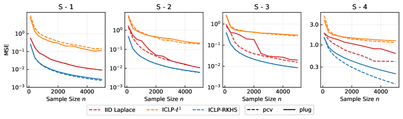
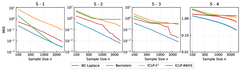
Figure 6: Plugin and PCV comparison (Top) and MSE for different mechanism (Bottom) for Matérn Kernel with $\alpha=\frac{5}{2}$ and $\rho=0.1$.

B.2 Visualization of Age-at-Death KDE

We present the visualization of the comparison between non-private KDE and private KDEs for different mechanisms in Figure 7.

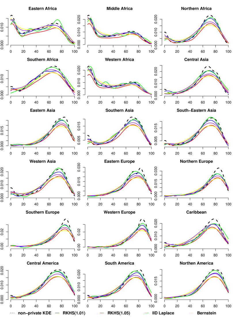
Figure 7: Non-private and private kernel density estimates of age-at-death density in different regions under different mechanisms with $\epsilon=1$.

References

• Alda and Rubinstein (2017) F. Alda and B. I. Rubinstein. The bernstein mechanism: Function release under differential privacy. In Thirty-First AAAI Conference on Artificial Intelligence, 2017.
• Awan and Slavković (2021) J. Awan and A. Slavković. Structure and sensitivity in differential privacy: Comparing k-norm mechanisms. Journal of the American Statistical Association, 116(534):935–954, 2021.
• Awan et al. (2019) J. Awan, A. Kenney, M. Reimherr, and A. Slavković. Benefits and pitfalls of the exponential mechanism with applications to hilbert spaces and functional pca. In International Conference on Machine Learning, pages 374–384. PMLR, 2019.
• Bogachev (1998) V. I. Bogachev. Gaussian measures. Number 62. American Mathematical Soc., 1998.
• Bosq (2000) D. Bosq. Linear processes in function spaces: theory and applications, volume 149. Springer Science & Business Media, 2000.
• Bousquet and Elisseeff (2002) O. Bousquet and A. Elisseeff. Stability and generalization. The Journal of Machine Learning Research, 2:499–526, 2002.
• Chandrasekaran et al. (2014) K. Chandrasekaran, J. Thaler, J. Ullman, and A. Wan. Faster private release of marginals on small databases. In Proceedings of the 5th conference on Innovations in theoretical computer science, pages 387–402, 2014.
• Chaudhuri and Vinterbo (2013) K. Chaudhuri and S. A. Vinterbo. A stability-based validation procedure for differentially private machine learning. Advances in Neural Information Processing Systems, 26:2652–2660, 2013.
• Chaudhuri et al. (2011) K. Chaudhuri, C. Monteleoni, and A. D. Sarwate. Differentially private empirical risk minimization. Journal of Machine Learning Research, 12(3), 2011.
• Cressie and Huang (1999) N. Cressie and H.-C. Huang. Classes of nonseparable, spatio-temporal stationary covariance functions. Journal of the American Statistical association, 94(448):1330–1339, 1999.
• Dwork et al. (2006) C. Dwork, F. McSherry, K. Nissim, and A. Smith. Calibrating noise to sensitivity in private data analysis. In Theory of cryptography conference, pages 265–284. Springer, 2006.
• Dwork et al. (2014) C. Dwork, A. Roth, et al. The algorithmic foundations of differential privacy. Found. Trends Theor. Comput. Sci., 9(3-4):211–407, 2014.
• Ferraty and Romain (2011) F. Ferraty and Y. Romain. The Oxford handbook of functional data analaysis. Oxford University Press, 2011.
• Hall et al. (2013) R. Hall, A. Rinaldo, and L. Wasserman. Differential privacy for functions and functional data. The Journal of Machine Learning Research, 14(1):703–727, 2013.
• Hardt and Talwar (2010) M. Hardt and K. Talwar. On the geometry of differential privacy. In Proceedings of the forty-second ACM symposium on Theory of computing, pages 705–714, 2010.
• Kakutani (1948) S. Kakutani. On equivalence of infinite product measures. Annals of Mathematics, pages 214–224, 1948.
• Kimeldorf and Wahba (1971) G. Kimeldorf and G. Wahba. Some results on tchebycheffian spline functions. Journal of mathematical analysis and applications, 33(1):82–95, 1971.
• Kokoszka and Reimherr (2017) P. Kokoszka and M. Reimherr. Introduction to functional data analysis. Chapman and Hall/CRC, 2017.
• Kosambi (2016) D. Kosambi. Statistics in function space. In DD Kosambi, pages 115–123. Springer, 2016.
• McSherry and Talwar (2007) F. McSherry and K. Talwar. Mechanism design via differential privacy. In 48th Annual IEEE Symposium on Foundations of Computer Science (FOCS’07), pages 94–103. IEEE, 2007.
• Micchelli and Wahba (1979) C. A. Micchelli and G. Wahba. Design problems for optimal surface interpolation. Technical report, WISCONSIN UNIV-MADISON DEPT OF STATISTICS, 1979.
• Mirshani et al. (2019) A. Mirshani, M. Reimherr, and A. Slavković. Formal privacy for functional data with gaussian perturbations. In International Conference on Machine Learning, pages 4595–4604. PMLR, 2019.
• Phan et al. (2019) N. Phan, M. Vu, Y. Liu, R. Jin, D. Dou, X. Wu, and M. T. Thai. Heterogeneous gaussian mechanism: Preserving differential privacy in deep learning with provable robustness. arXiv preprint arXiv:1906.01444, 2019.
• Ramsay et al. (2005) J. Ramsay, J. Ramsay, B. Silverman, et al. Functional Data Analysis. Springer Science & Business Media, 2005.
• Rao and Scott (1992) J. Rao and A. Scott. A simple method for the analysis of clustered binary data. Biometrics, pages 577–585, 1992.
• Reimherr and Awan (2019) M. Reimherr and J. Awan. Elliptical perturbations for differential privacy. arXiv preprint arXiv:1905.09420, 2019.
• Sacks and Ylvisaker (1966) J. Sacks and D. Ylvisaker. Designs for regression problems with correlated errors. The Annals of Mathematical Statistics, 37(1):66–89, 1966.
• Sacks and Ylvisaker (1968) J. Sacks and D. Ylvisaker. Designs for regression problems with correlated errors: many parameters. The Annals of Mathematical Statistics, 39(1):49–69, 1968.
• Sacks and Ylvisaker (1970) J. Sacks and D. Ylvisaker. Designs for regression problems with correlated errors iii. The Annals of Mathematical Statistics, 41(6):2057–2074, 1970.
• Tao (2011) T. Tao. An introduction to measure theory, volume 126. American Mathematical Society Providence, RI, 2011.
• Wang et al. (2013) Z. Wang, K. Fan, J. Zhang, and L. Wang. Efficient algorithm for privately releasing smooth queries. In NIPS, pages 782–790. Citeseer, 2013.
• Wasserman (2006) L. Wasserman. All of nonparametric statistics. Springer Science & Business Media, 2006.
• Wasserman and Zhou (2010) L. Wasserman and S. Zhou. A statistical framework for differential privacy. Journal of the American Statistical Association, 105(489):375–389, 2010.
• Yuan and Cai (2010) M. Yuan and T. T. Cai. A reproducing kernel hilbert space approach to functional linear regression. The Annals of Statistics, 38(6):3412–3444, 2010.
• Zhang et al. (2012) J. Zhang, Z. Zhang, X. Xiao, Y. Yang, and M. Winslett. Functional mechanism: regression analysis under differential privacy. arXiv preprint arXiv:1208.0219, 2012.