Unsupervised evaluation of GAN sample quality:
Introducing the TTJac Score

Abstract

Evaluation metrics are essential for assessing the performance of generative models in image synthesis. However, existing metrics often involve high memory and time consumption as they compute the distance between generated samples and real data points. In our study, the new evaluation metric called the ”TTJac score” is proposed to measure the fidelity of individual synthesized images in a data-free manner. The study first establishes a theoretical approach to directly evaluate the generated sample density. Then, a method incorporating feature extractors and discrete function approximation through tensor train is introduced to effectively assess the quality of generated samples. Furthermore, the study demonstrates that this new metric can be used to improve the fidelity-variability trade-off when applying the truncation trick. The experimental results of applying the proposed metric to StyleGAN 2 and StyleGAN 2 ADA models on FFHQ, AFHQ-Wild, LSUN-Cars, and LSUN-Horse datasets are presented. The code used in this research will be made publicly available online for the research community to access and utilize.

Introduction

Advancements in Generative Adversarial Networks (GANs) (Goodfellow et al. 2014) have led to a wide range of applications, including image manipulation (Voynov and Babenko 2020; Shen et al. 2020; Härkönen et al. 2020), domain translation (Isola et al. 2017; Zhu et al. 2017; Choi et al. 2017, 2020; Kim et al. 2020), and image/video generation (Kim, Choi, and Uh 2022; Kim and Ha 2022; Karras, Laine, and Aila 2019; Karras et al. 2020b, a). GANs have demonstrated high-quality results in these tasks, as validated by standard evaluation metrics such as Fréchet inception distance (FID) (Heusel et al. 2018), kernel inception distance (KID) (Bińkowski et al. 2018), Precision (Kynkäänniemi et al. 2019), and Recall (Kynkäänniemi et al. 2019). These metrics are typically based on clustering real data points using the k-nearest neighbours algorithm. Initially, real images are passed through a feature extractor network to obtain meaningful embeddings, and pairwise distances to other real images are computed for the algorithm. In the evaluation stage, the fidelity of an individual sample is determined by computing its distance to the clusters of real manifold. However, this procedure can be computationally expensive and memory-intensive, particularly for large datasets, as all real embeddings need to be stored.

In order to overcome these challenges, this research introduces a novel metric for evaluating the quality of individual samples. Instead of assessing sample fidelity relative to the real manifold, this metric directly calculates the density of a sample by utilizing only the trained generator. The computation process involves evaluating the model Jacobian, which can be particularly demanding for high-resolution models. To mitigate the memory and time costs associated with this computation, feature extractors are employed to reduce the size of the Jacobian.

Furthermore, the proposed metric function is approximated on a discrete grid using tensor train decomposition. This approximation provides a significant reduction in inference time since the batch of sample scores is only required to compute the tensor decomposition stage. The evaluation procedure simply entails obtaining the value of decomposed tensor at specified indexes.

The proposed metric function also has an application in the sampling procedure, particularly as an enhancement for the truncation trick. The truncation trick (Brock, Donahue, and Simonyan 2019) operates by sorting samples based on the norm of the input vector, which can be effectively replaced by the TTJac score. This upgrade provides a better trade-off between fidelity and variability compared to the standard technique.

Figure 1: The general pipeline of the presented work involves several steps. Firstly, latent code samples $z$ are generated from a normal distribution, then the generated latent codes are passed through the generator network, which produces corresponding images $x$. The VGG feature extractor is employed to extract meaningful features $f$. After obtaining the features, the computation of feature density is carried out using generalized change of variables formula (Ben-Israel 1999). Finally, the metric score samples are approximated using the Tensor Train (TT) algorithm.

To evaluate the effectiveness of the proposed metric function, standard GAN models like StyleGAN 2 (Karras et al. 2020b) and StyleGAN 2 ADA (Karras et al. 2020a) were considered, using various datasets such as Flickr-Faces-HQ Dataset (FFHQ) (Karras, Laine, and Aila 2019), AFHQ Wild (Choi et al. 2020), LSUN Car (Yu et al. 2016), and LSUN Horse (Yu et al. 2016). In summary, the contributions of this paper include:

1. Introducing a new metric for sample evaluation that does not rely on dataset information.

2. Presenting a methodology for effective usage of the proposed metric, involving feature extractors and tensor train approximation.

3. Proposing a metric-based upgrade for the truncation trick, enabling a better trade-off between fidelity and variability.

Method

The primary component of a GAN model is the generator network, denoted as $G$, which generates an image $x$ from a given latent code (network input) $z$. Typically, the evaluation of individual sample quality $x=G(z)$ is performed using a realism score or trucnation trick.

The realism score requires access to a dataset to compute distances for the k-nearest neighbors algorithm, while truncation trick assesses sample fidelity based on the norm of the corresponding input vector. This approach allows for resampling latent codes that lie outside a chosen radius.

In contrast, we propose a metric function that defines the score based on the density of the generator output. We use the generalized change-of-variable formula (Ben-Israel 1999):

$$\rho(z)=\rho(x)\mathrm{Vol}(J)$$

where $J=dG(z)/dz$ represents the generator Jacobian. By taking the logarithm and making the appropriate substitution, the final expression for the score function is derived:

$$s(x)=\log\rho(x)=\log(\rho(z))-\log(\mathrm{Vol}(J))$$

where $\mathrm{Vol}(J)=\frac{1}{2}\log(\det(J^{T}J))=\sum\limits_{i=1}^{N}\log(\sigma_{i}(J))$, $\sigma_{i}(J)$ represents the $i$-th singular value of the Jacobian. Finally score function turns into:

$$s(x)=\log(\rho(z))-\sum\limits_{i=1}^{N}\log(\sigma_{i}(J))$$

At this stage, we considered the image density in pixel representation. Nevertheless, the proposed idea can be applied to an arbitrary representation of the image. This aspect is discussed in the next part.

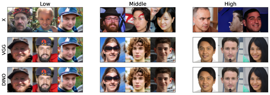
Figure 2: Qualitative comparison of different image features. Three types of output considered: original image (X), VGG19 features (VGG), Dino features (DINO). For each type the sample density was computed. Three images with low, middle, and high scores are presented for each output type.

Feature Density Scoring

High-resolution images can be generated by high-quality GANs (Generative Adversarial Networks). For instance, the StyleGAN2 model trained on the FFHQ dataset can generate images of size $1024\times 1024$ with a latent space size of 512. However, computing the Jacobian matrix, which contains $10^{9}$ values in this case, can be challenging in terms of both time and memory consumption.

To mitigate these costs, we propose to use feature extraction. Instead of evaluating sample quality based on pixel values, a score function can be used that assesses the density of features. The score function is defined as:

$$s(x)=\log\rho(f(x))=\log(\rho(z))-\log(\mathrm{Vol}(J))$$

Here, $J=\frac{df(G(z))}{dz}$ represents the Jacobian matrix, and $f$ denotes the feature extraction network. In Figure 1 we presented a whole pipeline of our work. The detailed explanations on last step delivered in next section.

In our work, we considered two options for the feature extraction network: VGG19(Simonyan and Zisserman 2015) and Dino(Caron et al. 2021). VGG networks are based on convolutional layers and have demonstrated high efficiency in classification tasks. They are widely used for extracting meaningful information from image data. On the other hand, Dino is a transformer-based network, which is known to be more accurate but has longer inference times compared to convolution-based networks.

To compare the performance of these feature extraction networks, we generated 100 images StyleGAN 2 ADA model trained on FFHQ dataset and evaluated the proposed metric. The experiments were conducted on a Tesla V100-SXM2 GPU with 16 GB of memory. Three types of output were considered: X (pixel-based density), VGG (VGG19-based feature density), and Dino (Dino-based feature density).

Feature extractor	Original	VGG	Dino
Time per sample (s)	450	25	90

Table 1: Comparison results of time consumption for metric inference. Three types of output density considered: Original - pixel based density, VGG - VGG features based density, Dino - Dino features based density

After conducting a sorting procedure, we selected three images with the lowest, middle, and highest scores for each output type. Figure 2 illustrates that VGG produces results that are comparable to pixel-based and Dino based density. Additionally, computing the VGG features-based density requires significantly less time per sample. For further experiments, we utilized VGG features for metric computation. Table 1 provides a comprehensive comparison of the time consumption for different output types.

Inference Time Acceleration through Tensor Train

Presented in previous section reduction in inference time is insufficient for the computation of a large number of samples. Currently, the computation of 50,000 scores takes around 2 weeks on a single GPU, even with the use of VGG based features. A potential solution to this problem is to discretize the metric on a grid and compress the resulting tensor using tensor decomposition. The proposed solution pipeline consists of two stages:

1. Score computation for a large number of samples

2. Computation of the logarithm density approximation using the samples obtained from the previous stage

To evaluate a sample $\hat{x}$ within this pipeline, the following steps can be followed:

1. Find the closest point to the latent code $\hat{z}$ in the discrete latent space $z[i_{1},...,i_{d}]$. This can be achieved by minimizing the Euclidean distance between the discrete latent codes and $\hat{z}$:

   $$(\hat{i}_{1},...,\hat{i}d)=\arg\min{(i_{1},...,i_{d})}\|z[i_{1},...,i_{d}]-\hat{z}\|$$

2. Compute the score value at this point using the density tensor $\rho[i_{1},...,i_{d}]$ stored in compressed format:

   $$s(\hat{x})=\rho[\hat{i}_{1},...,\hat{i}_{d}]$$

Non uniform grid

One crucial component in our scheme is the grid used for discretization. We found usage of a uniform grid is not suitable for GANs when sampling latent codes from a normal distribution. Certain latent regions may lack sufficient data, posing challenges for computation of tensor train descomposition.

To address this challenge, we opted for a grid where the integrals of the normal density over each grid interval are equal. This approach ensures a uniform distribution of samples along each grid index, effectively working in our case. More details can be found in Appendix A.

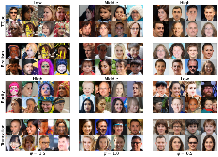
Figure 3: Qualitative comparison of metrics for individual image evaluation: TTJac score, Realism score, Rarity score, Truncation Trick. For each metric we presented 8 images with lowest, middle, and highest score values. For the TTJac and Realism scores, we arranged the images in increasing order from low to high scores. Conversely, for the Rarity score and Truncation Trick, we intentionally reversed the order to ensure ease of comparison between the metrics.

Domain	FFHQ	Wild	Car	Horse
MSE	0.018	0.026	0.017	0.018

Table 2: Quantitative evaluation of TT approximation of TTJac score on discrete grid for different domains: FFHQ, AFHQ-Wild, LSUN Car, LSUN Horse

Calculation of Tensor Train approximation

The TT decomposition of a tensor represents the element at position $[i_{1},...,i_{N}]$ as the product of matrices:

$$T[i_{1},...,i_{N}]=G_{1}[i_{1}]...G_{N}[i_{N}]$$

Here, $G_{1},...,G_{N}$ are the TT cores. The low-rank pairwise dependency between tensor components allows for an efficient approximation of the proposed metric function in discrete form using well known Tensor Train decomposition (Oseledets 2011). It showed impressive results on different tasks (Chertkov, Ryzhakov, and Oseledets 2023; Ahmadi-Asl et al. 2023; Liu et al. 2023; Li et al. 2023) due to the storage efficiency, capturing complex dependencies and fast inference capabilities. Obtaining an element of the tensor stored in TT format requires only $511$ matrix-by-vector multiplications. It also can be easily accelerated for the batch of elements using multiprocessing tools. Actually the batch size could be enormously large for TT format since it on each step of output computation algorithm stores the matrix of size $(N,r)$ where $N$ number of elements to compute, $r$ - rank of decomposition. This aspect has significat impact on use of proposed metric for truncation trick, where we need to evaluate huge number of samples.

However, it should be noted that the computation of samples for core computation is time-consuming. This renders standard iterative methods for tensor train calculation ineffective, as they tend to overfit to given tensor samples and fail to capture underlined dependencies. In such case, it is more suitable to use explicit methods for tensor train decompositions, such as ANOVA decomposition (Potts and Schmischke 2021). The authors in (Chertkov, Ryzhakov, and Oseledets 2023) have presented an effective method for computing ANOVA decomposition in TT format, which we have found accurate enough for our purposes. See Table 2 where we presented the results of TT approximation for discretized metric in different domains.

Upgraded Truncation Trick

The truncation trick, initially proposed in (Brock, Donahue, and Simonyan 2019), offers a means to adjust the balance between variability and fidelity. It involves two practical steps: evaluating the norm of generated samples and resampling those with a norm exceeding a specified threshold. This threshold determines the balance between variability and fidelity. By removing samples with high norms, we effectively reduce the number of samples with low latent code density and, possibly, lower visual quality. This approach can enhance the overall fidelity of the generated samples, albeit at the expense of variability.

Instead of evaluating latent code density, we suggest assessing image feature density using a modern feature extractor such as VGG. In next section, we provide evidence that this replacement criterion achieves a more desirable trade-off between fidelity and variability.

Experiment

To evaluate the proposed metric, we conducted experiments on various widely-used datasets for image generation, including FFHQ (Karras, Laine, and Aila 2019), AFHQ-Wild (Choi et al. 2020), LSUN-Cars (Yu et al. 2016), and LSUN-Horse (Yu et al. 2016). Additionally, we considered the method effectiveness on StyleGAN 2 (Karras et al. 2020b) and StyleGAN 2 ADA (Karras et al. 2020a) models, known for their high performance in generating images in standard domains where data may be limited or noisy.

For the learning process of the metric, we computed $60k$ samples for the FFHQ dataset and $30k$ samples for the AFHQ-Wild, LSUN-Cars, and LSUN-Horse datasets. Feature extraction was performed using the VGG19 network (Simonyan and Zisserman 2015).

To discretize the metric, we utilized a grid with a size of $32$. The metric was then approximated by applying ANOVA decomposition of order 1, which was later converted to the tensor train format.

All experiments were carried out using a 3 Tesla V100-SXM2 GPU with 16 GB of memory.

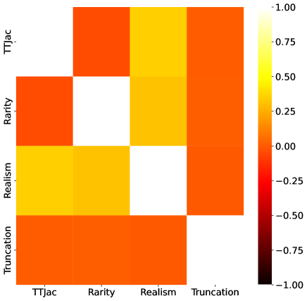
Figure 4: Correlation matrix for metrics measuring individual sample quality: TTJac score, Realism score, Rarity score, and Truncation.

Number of border samples	Rarity	Realism	Truncation
3000	-0.051	0.42	0.007
2000	-0.059	0.472	0.156
1000	-0.048	0.54	0.006
500	-0.048	0.584	0.049
100	-0.043	0.651	0.135

Table 3: Quantitative results of correlation between TTJac score and other considered metrics: Rarity score, Realism score, Truncation. Computation was done for certain number of samples representing the higher and lower extremes of the TTJac score - border samples.

Comparison with other metrics

To demonstrate the effectiveness of the TTJac score in evaluating individual samples, we compared it with similar metrics such as the Realism score (Kynkäänniemi et al. 2019), Truncation trick (Brock, Donahue, and Simonyan 2019), and Rarity score (Han et al. 2022). We randomly selected $10k$ latent samples and presented the comparison results in Figure 3.

In order to facilitate the comparison process, we reversed the order for the Rarity score and Truncation. The Realism score showed high results in evaluating sample fidelity but sometimes failed on visually appealing images. It is important to note that high realism values often correspond to images with low variability. Similarly, the Truncation trick allows for manipulation of image quality at the expense of variability. However, samples with the highest variability tend to have lower realism compared to other metrics. On the other hand, the Rarity score measures the uniqueness of the given image, effectively identifying images with distinct features, but some of them may appear less realistic.

The proposed TTJac score functions similarly to the realism score but does not require any real data for processing. It effectively extracts samples with high fidelity, reflected by a high score. Conversely, low scores often indicate the presence of visual artifacts. However, the TTJac score does have a limitation – images with high scores tend to have fewer unique features, while visually appealing images can be found among those with low scores.

We also computed the correlation between the presented metrics. The results confirmed quite high similarity between the realism and TTJac scores, as shown in Figure 4. Furthermore, when measuring metrics correlation for samples with the highest and lowest TTJac scores, results of proposed metric becomes even more close to realism score. See Table 3 for confirmation. Thus, the data free metric TTJac is able to filter out very low quality images as effectively as the Realism score using a dataset of real images.

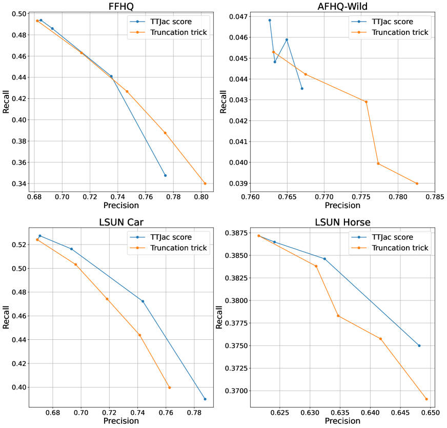
Figure 5: Quantitative comparison of fidelity-variability trade-off computed using TTJac score and Truncation trick. Four domains were examined: FFHQ, AFHQ-Wild, LSUN Car, LSUN Horse. For each domain $50k$ samples were generated for precision and recall calculation. The results were averaged along 3 random seeds. The higher - the better.

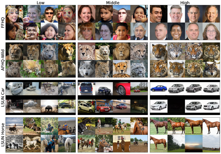
Figure 6: Qualitative comparison of metric evaluation capabilities four domains were examined: FFHQ, AFHQ-Wild, LSUN Car, LSUN Horse. For each domain $30k$ samples were sorted based on their scores and selected three images to represent the samples with the lowest, middle, and highest score values.

Fidelity-variability trade-off evaluation

In method section, we discussed the potential use of the proposed metric to enhance the performance of the truncation trick. In this section, we compare the trade-off provided by the standard criteria based on latent code norm, and the TTJac score. To demonstrate the effectiveness, we plotted precision-recall curves for the FFHQ, AFHQ-Wild, LSUN-Car, and LSUN-Horse domains.

For the FFHQ, LSUN Horse, and LSUN Car domains, the use of the TTJac score allows for a better balance between precision and recall compared to the standard tool. In Figure 5, the curve for the TTJac score consistently lies above the curve for the Truncation trick. The benefit is not significant for the AFHQ-Wild domain. This can be attributed to the fact that the GAN model already exhibits a high level of precision in this specific domain. Furthermore, the evaluation of TT approximation accuracy presented the least favorable outcome when compared to other domains. And also on the FFHQ domain, after an improvement in precision by 5%, a decline begins and the curve falls below that for the standard truncation trick. It can be attributed to the presence of an error in the metric approximation. However, for the LSUN-Car domain, the TTJac score proves to be highly effective, providing a significant improvement in precision with negligible loss in recall.

It is important to note that due to the presence of errors in the approximation of the metric score, it is not possible to achieve the maximum possible precision with minimal recall value, as seen in standard precision-recall curves.

Overall, this comparison highlights the potential of the TTJac score in achieving a better trade-off between precision and recall in the evaluated domains, with notable improvements observed in the LSUN-Car domain.

Domain wise metric evaluation

In this part, we conducted a qualitative evaluation of the TTJac score for various domains. In Figure 6, it is demonstrated that the TTJac score efficiently detects visual artifacts in the evaluated domains.

For the FFHQ domain, the TTJac score assigns low scores to images that do not contain a face or have unrealistic prints. Additionally, images with visually poor backgrounds are also marked with low score values. Similarly, in the LSUN Car domain, images that lack key elements of a car are identified as lower quality by the TTJac score.

The TTJac score exhibits similar behavior in the AFHQ-Wild and LSUN-Horse domains. It effectively detects unrealistic horses, such as instances where two horses are merged into one image. However, in the AFHQ-Wild domain, the metric faces a more challenging situation. While it accurately identifies images where different species are merged, such as an image with half wolf and half lion, the overall fidelity of the images in this domain is quite close. This observation is connected to the fact that the model trained on the AFHQ-Wild dataset has a higher precision compared to the other considered models.

In summary, the TTJac score demonstrates high efficiency in evaluating sample fidelity while sacrificing some variability. It effectively detects visual artifacts and accurately identifies unrealistic elements in the evaluated domains.

Conclusion

We have proposed a new approach for evaluating image quality without using real data, which is based on the density of meaningful features extracted from the image. A method was also proposed for efficient storage and inference metrics using TT approximation. We compared the TTJac score with other metrics. The TTJac score performs similarly to the realism score. It effectively detects visual artifacts and identifies unrealistic elements in different domains such as FFHQ, AFHQ-Wild, LSUN Car, and LSUN Horse. We also evaluated the trade-off between fidelity and variability using precision-recall curves. The TTJac score showed a better balance, especially in the LSUN Car domain where it significantly improved precision with minimal loss in recall. In qualitative evaluation, the TTJac score successfully detected missing key elements or unrealistic features in images across various domains. Overall, the TTJac score demonstrates high efficiency in evaluating sample fidelity and can be a valuable tool for assessing image generation models.

.

Appendix A Appendix A

The general representation of a tensor $T$ in the TT format is:

$$T[i_{1},...,i_{d}]\approx G_{1}[i_{1}]G_{2}[i_{2}]...G_{d}[i_{d}]$$

Here, $G_{1},...,G_{d}$ are matrices of size $(r,r)$ (if the compression rank is equal), and $d$ is the size of the latent space.

The most common way to find the cores $G_{k}$ for a tensor represented by random elements is the alternative least squares algorithm (ALS) (Holtz, Rohwedder, and Schneider 2012). This algorithm consists of an alternating best fit for each of the cores $G_{k}$ in the order of $k=1,...,d$. For each core $G_{k}$, we need to solve an independent least squares problem:

$$\hat{G}k=\arg\min{G_{k}}|T-[G_{1},...,G_{k},...G_{d}]|$$

Here, $[G_{1},...,G_{k},...G_{d}]$ is a short notation for the tensor represented in the TT format, and $\hat{G}_{k}$ is the solution for the least squares problem. This problem can be solved independently for each matrix $G_{k}[i]$, where $i=1,...,N$ (N is the grid size):

$$\hat{G}_{k}[i]=\arg\min{G_{k}[i]}\|T^{k}_{i}-L_{k}G_{k}[i]R_{k}\|$$

In the above equation, $L_{k}[i_{1},...,i_{k-1}]=G_{1}[i_{1}]...G_{k-1}[i_{k-1}]$ left side of TT format for core $k$, $R_{k}[i_{k+1},...,i_{d}]=G_{k+1}[i_{k+1}]...G_{d}[i_{d}]$ right side of TT format for core $k$, and $T^{k}_{i}[i_{1},...,i_{k-1},i_{k+1},...,i_{d}]=T[i_{1},...,i_{k}=i,...,i_{d}]$ represents a $(d-1)$-dimensional target tensor.

If we have $M$ tensor elements, then $L_{k}$ becomes a set of vectors $L_{k}[m]=L_{k}[i_{1}=i_{1}^{m},...,i_{k-1}=i_{k-1}^{m}]$ representing the left side of the TT format for $m=1,...,M$ samples, $i_{1}^{m},...,i_{d}^{m}$ - indexes of $m$-th tensor sample. $R_{k}$ similarly turns into a corresponding set of vectors $R_{k}[m]=R_{k}[i_{k+1}=i_{k+1}^{m},...,i_{d}=i_{d}^{m}]$. Both $L_{k}$ and $R_{k}$ here have size $(M_{i}^{k},r)$, where $M_{i}^{k}$ represents the number of samples for which $i_{k}=i$. In this case, $T^{k}_{i}$ becomes a vector of values of tensor samples corresponding to $i_{k}=i$. Finally the problem can then be formulated as a standard linear problem:

$$\hat{G}_{k}[i]=\arg\min{G_{k}[i]}\|T^{k}_{i}-(R_{k}\odot L_{k})\mathrm{vec}(G_{k}[i])\|$$

In the above equation, $R_{k}\odot L_{k}$ represents the face-splitting product of matrices $L_{k}$ and $R_{k}$ of size $(M_{i}^{k},r^{2})$, and $\mathrm{vec}(G_{k}[i])$ represents the vectorization of matrix $G_{k}[i]$. To solve the problem, $M_{i}^{k}$ should be greater than or equal to $r^{2}$ for any $k$ and $i$. If this condition is not met, the system becomes underdetermined, necessitating the setting of additional constraints.

This is the main problem where the grid type affects tensor decomposition. Let us consider a uniform grid with the following parameters: minimal value $a=-3$, maximal value $b=3$, and grid size $N=64$. For a normally distributed variable $z_{k}$, the relative number of samples inside interval $[t_{i},t_{i+1}]$ is given by:

$$p^{k}_{i}=\frac{\int_{t_{i}}^{t_{i+1}}\exp(-z_{k}^{2}/2)}{\int_{t_{0}}^{t_{N-1}}\exp(-z_{k}^{2}/2)}$$

Here, $t_{i}=a+\frac{(b-a)}{(N-1)}i$, and $i$ represents the grid index in the range $[0,N-1]$.

Based on this, we can find the ratio between the number of samples inside the first interval $i=0$ and the middle one $i=N/2-1=31$:

$$\frac{p^{k}_{0}}{p^{k}_{31}}=0.013$$

The discrepancy in the number of equations between $i=0$ and $i=31$ poses a limitation on the rank of the decomposition. For $i=31$, the system has approximately 100 times more equations compared to $i=0$. Additionally, when considering the total number of samples $M=50k$, on average, only 24 samples have $i=0$ restricting the rank of the decomposition to a maximum of 4.

To address this issue, we propose using a non-uniform grid with intervals $[t_{0},t_{1}],[t_{1},t_{2}],...,[t_{N-2},t_{N-1}]$ such that the integral of the normal density over these intervals is equal:

$$\int_{t_{i}}^{t_{i+1}}\exp\left(-\frac{z_{k}^{2}}{2}\right)=\int_{t_{j}}^{t_{j+1}}\exp\left(-\frac{z_{k}^{2}}{2}\right)$$

Here, $i$ and $j$ can be any arbitrary values in the range $[0,N-2]$. By imposing this condition on grid points, the number of equations in the linear system becomes equal for all values of $i$.

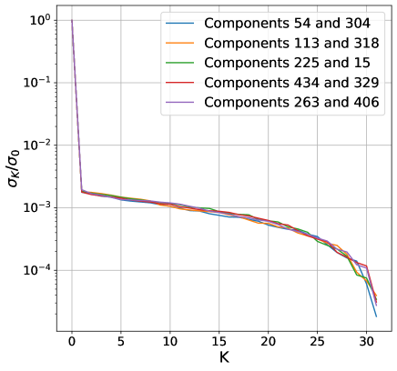
Figure 7: Normalized cumulative sum of singular values for matrix $C$ computed for random pairs of components

Appendix B Appendix B

Computation of tensor train cores rise a question of choosing optimal hyperparameters like rank, method, core initialization, number of iterations (if applicable). To find the optimal rank we constructed the matrix $C$ describing the pair wise dependency between two components $k_{1}$ and $k_{2}$:

$$C[j_{r},j_{c}]=\mathop{\mathbb{E}}\limits_{i_{k},k\neq[k_{1},k_{2}]}T[i_{1},...,i_{k_{1}}=j_{r},...,i_{k_{2}}=j_{c},...,i_{d}]$$

where $C[j_{r},j_{c}]$ - the element on intersection of $j_{r}$-th row and $j_{c}$-th column. Taking into consideration the TT approximation $T\approx[G_{1},...,G_{d}]$ we can express previous equation from TT format side:

$$C[j_{r},j_{c}]\approx\mathop{\mathbb{E}}\limits_{i_{k},k\neq[k_{1},k_{2}]}G_{1}[i_{1}]...G_{k_{1}}[i_{k_{1}}=j_{r}]...\\ G_{k_{2}}[i_{k_{2}}=j_{c}]...G_{d}[i_{d}]$$

Here $G_{1}$ is a vector (first TT core). Summation made along second dimension of each core produces the following result:

$$C[j_{r},j_{c}]\approx G_{1}^{k_{1}-1}G_{k_{1}}[i_{k_{1}}=j_{r}]G_{k_{1}+1}^{k_{2}-1}G_{k_{2}}[i_{k_{2}}=j_{c}]G_{k_{2}+1}^{d}$$

where $G_{1}^{k_{1}-1}$ is a vector representing product of averaged along middle dimension cores before $k_{1}$ component, $G_{k_{1}+1}^{k_{2}-1}$ is a matrix of size $(r,r)$ representing product of averaged along middle dimension cores after $k_{1}$ and before $k_{2}$ components, $G_{k_{2}+1}^{d}$ is a vector representing product of averaged along middle dimension cores after $k_{2}$ component.

The rank of matrix $C$ is equal to $\mathrm{rank}(G_{1}^{k_{1}-1}G_{k_{1}}G_{k_{1}+1}^{k_{2}-1}G_{k_{2}}G_{k_{2}+1}^{d})\leq r$ since the smallest dimension size of tensors in the product is $r$. So following this formulation we could estimate the optimal rank by evaluating the rank of matrix $C$ computed for target tensor $T$. Figure 7 presents normalized singular values for matrix $C$ computed for different random pairs of tensor components. Based on results we can conclude that tensor could be accurately compressed with small rank.

References

- Ahmadi-Asl et al. (2023) Ahmadi-Asl, S.; Asante-Mensah, M. G.; Cichocki, A.; Phan, A. H.; Oseledets, I.; and Wang, J. 2023. Fast cross tensor approximation for image and video completion. Signal Processing, 109121.
- Ben-Israel (1999) Ben-Israel, A. 1999. The Change-of-Variables Formula Using Matrix Volume. Siam Journal on Matrix Analysis and Applications - SIAM J MATRIX ANAL APPLICAT, 21.
- Bińkowski et al. (2018) Bińkowski, M.; Sutherland, D. J.; Arbel, M.; and Gretton, A. 2018. Demystifying MMD GANs.
- Brock, Donahue, and Simonyan (2019) Brock, A.; Donahue, J.; and Simonyan, K. 2019. Large Scale GAN Training for High Fidelity Natural Image Synthesis. In International Conference on Learning Representations.
- Caron et al. (2021) Caron, M.; Touvron, H.; Misra, I.; Jégou, H.; Mairal, J.; Bojanowski, P.; and Joulin, A. 2021. Emerging Properties in Self-Supervised Vision Transformers. In Proceedings of the International Conference on Computer Vision (ICCV).
- Chertkov, Ryzhakov, and Oseledets (2023) Chertkov, A.; Ryzhakov, G.; and Oseledets, I. 2023. Black Box Approximation in the Tensor Train Format Initialized by ANOVA Decomposition. SIAM Journal on Scientific Computing, 45(4): A2101–A2118.
- Choi et al. (2017) Choi, Y.; Choi, M.; Kim, M.; Ha, J.-W.; Kim, S.; and Choo, J. 2017. StarGAN: Unified Generative Adversarial Networks for Multi-Domain Image-to-Image Translation. arXiv preprint arXiv:1711.09020.
- Choi et al. (2020) Choi, Y.; Uh, Y.; Yoo, J.; and Ha, J.-W. 2020. StarGAN v2: Diverse Image Synthesis for Multiple Domains. In Proceedings of the IEEE Conference on Computer Vision and Pattern Recognition.
- Goodfellow et al. (2014) Goodfellow, I.; Pouget-Abadie, J.; Mirza, M.; Xu, B.; Warde-Farley, D.; Ozair, S.; Courville, A.; and Bengio, Y. 2014. Generative Adversarial Nets. In Ghahramani, Z.; Welling, M.; Cortes, C.; Lawrence, N.; and Weinberger, K., eds., Advances in Neural Information Processing Systems, volume 27. Curran Associates, Inc.
- Han et al. (2022) Han, J.; Choi, H.; Choi, Y.; Kim, J.; Ha, J.-W.; and Choi, J. 2022. Rarity Score: A New Metric to Evaluate the Uncommonness of Synthesized Images. arXiv preprint arXiv:2206.08549.
- Heusel et al. (2018) Heusel, M.; Ramsauer, H.; Unterthiner, T.; Nessler, B.; and Hochreiter, S. 2018. GANs Trained by a Two Time-Scale Update Rule Converge to a Local Nash Equilibrium. arXiv:1706.08500.
- Holtz, Rohwedder, and Schneider (2012) Holtz, S.; Rohwedder, T.; and Schneider, R. 2012. The Alternating Linear Scheme for Tensor Optimization in the Tensor Train Format. SIAM J. Sci. Comput., 34.
- Härkönen et al. (2020) Härkönen, E.; Hertzmann, A.; Lehtinen, J.; and Paris, S. 2020. GANSpace: Discovering Interpretable GAN Controls. In Proc. NeurIPS.
- Isola et al. (2017) Isola, P.; Zhu, J.-Y.; Zhou, T.; and Efros, A. A. 2017. Image-to-Image Translation with Conditional Adversarial Networks. CVPR.
- Karras et al. (2020a) Karras, T.; Aittala, M.; Hellsten, J.; Laine, S.; Lehtinen, J.; and Aila, T. 2020a. Training Generative Adversarial Networks with Limited Data. In Proc. NeurIPS.
- Karras, Laine, and Aila (2019) Karras, T.; Laine, S.; and Aila, T. 2019. A Style-Based Generator Architecture for Generative Adversarial Networks. In 2019 IEEE/CVF Conference on Computer Vision and Pattern Recognition (CVPR), 4396–4405.
- Karras et al. (2020b) Karras, T.; Laine, S.; Aittala, M.; Hellsten, J.; Lehtinen, J.; and Aila, T. 2020b. Analyzing and Improving the Image Quality of StyleGAN. In 2020 IEEE/CVF Conference on Computer Vision and Pattern Recognition (CVPR), 8107–8116.
- Kim, Choi, and Uh (2022) Kim, J.; Choi, Y.; and Uh, Y. 2022. Feature Statistics Mixing Regularization for Generative Adversarial Networks. In CVPR.
- Kim et al. (2020) Kim, J.; Kim, M.; Kang, H.; and Lee, K. H. 2020. U-GAT-IT: Unsupervised Generative Attentional Networks with Adaptive Layer-Instance Normalization for Image-to-Image Translation. In International Conference on Learning Representations.
- Kim and Ha (2022) Kim, Y.; and Ha, J.-W. 2022. Contrastive Fine-grained Class Clustering via Generative Adversarial Networks.
- Kynkäänniemi et al. (2019) Kynkäänniemi, T.; Karras, T.; Laine, S.; Lehtinen, J.; and Aila, T. 2019. Improved Precision and Recall Metric for Assessing Generative Models. CoRR, abs/1904.06991.
- Li et al. (2023) Li, S.; Wang, Z.; Yau, S. S.-T.; and Zhang, Z. 2023. Solving Nonlinear Filtering Problems Using a Tensor Train Decomposition Method. IEEE Transactions on Automatic Control, 68: 4405–4412.
- Liu et al. (2023) Liu, H.; Wang, J.; Yin, X.; Ding, J.; Yang, L. T.; Yao, T.; Yang, J.; and Gao, Y. 2023. Tensor-Train-Based Multiuser Multivariate Multiorder Physical Markov Process Informed Multimodal Prediction for Industrial Trajectory Applications. IEEE Transactions on Industrial Informatics, 19: 8900–8909.
- Oseledets (2011) Oseledets, I. V. 2011. Tensor-Train Decomposition. SIAM Journal on Scientific Computing, 33(5): 2295–2317.
- Potts and Schmischke (2021) Potts, D.; and Schmischke, M. 2021. Approximation of high-dimensional periodic functions with Fourier-based methods. arXiv:1907.11412.
- Shen et al. (2020) Shen, Y.; Gu, J.; Tang, X.; and Zhou, B. 2020. Interpreting the Latent Space of GANs for Semantic Face Editing. In CVPR.
- Simonyan and Zisserman (2015) Simonyan, K.; and Zisserman, A. 2015. Very Deep Convolutional Networks for Large-Scale Image Recognition. arXiv:1409.1556.
- Voynov and Babenko (2020) Voynov, A.; and Babenko, A. 2020. Unsupervised discovery of interpretable directions in the gan latent space. In International Conference on Machine Learning, 9786–9796. PMLR.
- Yu et al. (2016) Yu, F.; Seff, A.; Zhang, Y.; Song, S.; Funkhouser, T.; and Xiao, J. 2016. LSUN: Construction of a Large-scale Image Dataset using Deep Learning with Humans in the Loop. arXiv:1506.03365.
- Zhu et al. (2017) Zhu, J.-Y.; Park, T.; Isola, P.; and Efros, A. A. 2017. Unpaired Image-to-Image Translation using Cycle-Consistent Adversarial Networks. In Computer Vision (ICCV), 2017 IEEE International Conference on.
.