Boundary Control and Observer Design Via Backstepping for a Coupled Parabolic-Elliptic System

Abstract

Stabilization of a coupled system consisting of a parabolic partial differential equation and an elliptic partial differential equation is considered. Even in the situation when the parabolic equation is exponentially stable on its own, the coupling between the two equations can cause instability in the overall system. A backstepping approach is used to derive a boundary control input that stabilizes the coupled system. The result is an explicit expression for the stabilizing control law. The second part of the paper involves the design of exponentially convergent observers to estimate the state of the coupled system, given some partial boundary measurements. The observation error system is shown to be exponentially stable, again by employing a backstepping method. This leads to the design of observer gains in closed-form. Finally, we address the output-feedback problem by combining the observers with the state feedback boundary control. The theoretical results are demonstrated with numerical simulations.

,

1 Introduction

The coupling of parabolic partial differential equations with elliptic partial differential equations appears in a number of physical applications, including electro-chemical models of lithium-ion cells [9, 34], biological transport networks [17], chemotaxis phenomena [2, 22] and the thermistor [19]. Parabolic-elliptic systems are thus an important class of partial differential-algebraic equations (PDAEs). Well-posedness of linear PDAEs has been addressed in the literature [30, 28, 26, 12]. There have also been research efforts dedicated to investigate the well-posdeness of particular linear parabolic-elliptic systems [2, 7]. In addition, the well-posedness of quasilinear and nonlinear parabolic-elliptic systems have received a recent attention; see [33, 22, 8, 18, 17].

Parabolic-elliptic systems can exhibit instability, leading to several complications in real-life applications. One example can be found in the context of chemotaxis phenomena. In this case the parabolic equation describes the diffusion of cells while the elliptic equation models the concentration of a chemical attractant. In [27] authors showed that the aforementioned model can manifest unstable dynamics, leading to spatially complex patterns in cell density as well as the concentration of the chemical; see [24]. These patterns will in turn impact many biological processes including tissue development, tumor growth and wound healing. A more recent illustration for the instability in coupled parabolic-elliptic systems can be found in [23]. The findings in this paper demonstrated that even when the parabolic equation is exponentially stable, coupling with the elliptic equation can lead to an unstable system.

Stabilization through boundary control for coupled linear parabolic partial differential equations has been studied in the literature. In [6], the backstepping approach was used to stabilize the dynamics of a linear coupled reaction-diffusion systems with constant coefficients. An extension of this work to systems with variable coefficients was presented in [31]. Koga et al. [14] described boundary control of the one phase Stefan problem, modeled by a diffusion equation coupled with an ordinary differential equation. Feedback stabilization of a PDE-ODE system was also studied in [11].

There is less research tackling the stabilization of coupled parabolic-elliptic systems. [16, 15, 23]. In [16, chap. 10], stabilization of parabolic-elliptic systems arose in the context of stabilizing boundary control of linearized Kuramoto-Sivashinsky and Korteweg de Vries equations. The controller required the presence of two Dirichlet control inputs. A similar approach was also followed in [15] where a hyperbolic-elliptic system arose in the control of a Timoshenko beam. More recently, Parada et al. [23] considered the boundary control of unstable parabolic-elliptic system through Dirichlet control with input delay.

The first main contribution of this paper is design of a single feedback Neumann control input that exponentially stabilizes the dynamics of the two coupled equations. The control input is directly designed on the system of partial differential equations without approximation by finite-dimensional systems. This will be done by a backstepping approach [16]. Backstepping is one of the few methods that yields an explicit control law for PDEs without first approximating the PDE. These transformations are generally formulated as a Volterra operator, which guarantees under weak conditions the invertibility of the transformation. When using backstepping, it is typical to determine the destabilizing terms in the system, find a suitable exponentially stable target system where the destabilizing terms are eliminated by state transformation and feedback control. Then, look for an invertible state transformation of the original system into the exponentially stable target system. This requires finding a kernel of the Volterra operator and also showing that the kernel is well-defined as the solution of an auxilary PDE. One possible approach for stabilization of a parabolic-elliptic system is to convert the coupled system into one equation in terms of the parabolic state. However, this will result in the presence of a Fredholm operator that makes it difficult to establish a suitable kernel for the backstepping transformation. Another approach would be a vector-valued transformation for both of the parabolic and the elliptic states but this is quite complex. A different approach is taken here. We use a single transformation previously used for a parabolic equation [16]. Properties of the kernel of this transformation have already been established. This leads to an unusual target system in a parabolic-elliptic form. As in other backstepping designs, an explicit expression for the controller is obtained as a byproduct of the transformation. Then the problem is to establish the stability of the target system obtained from the transformation, which will imply the stability of the original coupled system via the invertible transformation. Explicit calculation of the eigenfunctions is not required.

In many dynamical systems, the full state is not available. This issue motivated the study of constructing an estimate of the state by designing an observer. The literature on observer design for coupled systems appears to focus on the observer synthesis of systems governed by coupled hyperbolic PDEs or coupled parabolic PDEs; see for instance [1, 21, 32, 5]. There have been few papers addressing observer design problem for partial differential equations coupled with an elliptic equation [13, 15]. In [13] authors designed a state observer for a coupled parabolic-elliptic system by requiring a two-sided boundary input for the observer. Also, in the same work mentioned earlier for Timoshenko beam [15], authors studied its observer design by using a hyperbolic-elliptic system and requiring two control inputs. In [25] an observer is designed for a parabolic equation that includes a Volterra term. We design an observer using two measurements, and also several observers that require only one measurement. The exponential stability of the observation error dynamics is achieved by means of designing suitable output injections, also known as filters or observer gains. In parallel to our approach for the boundary controller design, we derive observer gains by using backstepping transformations that are well-established in the literature. The transformations result in target error systems whose stability is studied.

We finally combine the state feedback and observer designs to obtain an output feedback controller for the coupled parabolic-elliptic system. Numerical simulations are presented that illustrate the theoretical findings for each of the objectives. To our knowledge, this paper is the first to designing a state estimator for a coupled parabolic-elliptic system with partial boundary measurements, and only one control input.

This paper is structured as follows. Section 2 presents the well-posedness of the parabolic-elliptic systems under consideration. Stability analysis for the uncontrolled system is also described. Section 3 includes the first main result which is the use of a backstepping method to design a boundary controller for the coupled system. A preliminary version of section 3, on stabilization, is included in the proceedings of the 2023 Conference on Decision and Control [3]. The design of a state observer for the coupled system is given in Section 4. Different designs are proposed based on the available measurements. The output feedback problem is described in Section 5. Conclusions and some discussion of possible extensions are given in Section 6.

2 Well-posedness and stability of system

We study parabolic-elliptic systems of the form

$$w_{t}(x,t)= w_{xx}(x,t)-\rho w(x,t)+\alpha v(x,t),$$ (1)

$$0= v_{xx}(x,t)-\gamma v(x,t)+\beta w(x,t),$$ (2)

$$w_{x}(0,t)= 0,\quad w_{x}(1,t)=u(t),$$ (3)

$$v_{x}(0,t)= 0,\quad v_{x}(1,t)=0,$$ (4)

where $x\in[0,1]$ and $t\geq 0$. The parameters $\rho,\;\alpha,\;\beta,\;\gamma$ are all real, with $\alpha$, $\beta$ both nonzero.

With the notation $\Delta v(x)=\frac{d^{2}v}{dx},$ define the operator $A^{\gamma}:D(A^{\gamma})\to L^{2}(0,1)$

$$A^{\gamma}v(x)=(\gamma I-\Delta)v(x)=w(x),$$

$$D(A^{\gamma})=\{v\in H^{2}(0,1),\;v^{\prime}(0)=v^{\prime}(1)=0\}.$$

For values of $\gamma$ that are not eigenvalues of $A^{\gamma}$, that is $\gamma\neq-n\pi^{2}$ with $n=0,\dots$, the inverse operator of $A^{\gamma}$ $(A^{\gamma})^{-1}:L^{2}(0,1)\to D(A^{\gamma})$ exists. In this situation, the uncontrolled system (1)-(4) is well-posed [12]. Alternatively, define

$$A=\Delta-\rho I+\alpha\beta(\gamma I-\Delta)^{-1},$$ (5)

$$D(A)=\{w\in H^{2}(0,1),\;w^{\prime}(0)=w^{\prime}(1)=0\}.$$

Theorem 1.

If $\gamma\neq-(n\pi)^{2}$ the operator $A$ generates a $C_{0}$- semigroup and the control system (1)-(4) with observation $w(0,t)$ is well-posed on the state-space $L^{2}(0,1).$ It is similarly well-posed with control instead at $x=0$, and/or observation at $x=1.$

Proof. With $\alpha=0$ the control system is the heat equation with Neumann boundary control. This control system is well-known to be well-posed on $L^{2}(0,1)$ . Since the operator $A$ is a bounded perturbation of $\Delta$, then the conclusion of the theorem follows. $\hfill\square$

It will henceforth be assumed that $\gamma\neq-(n\pi)^{2}.$

Theorem 2.

Let $u(t)\equiv 0$. The eigenvalues of system (1)-(4) operator $A$ are

$$\lambda_{n}=-\rho+\frac{\alpha\beta}{\gamma+(n\pi)^{2}}-(n\pi)^{2},\;\;n=0,\;1,\;\dots$$ (6)

Proof. The analysis is standard but given for completeness. Let $\{\phi_{j}\}_{j\geq 0}\subset\mathcal{C}^{4}(0,1)$ be the eigenfunctions of the operator $A$ corresponding to the eigenvalues $\lambda_{j}$, then setting $\beta(\gamma I-\partial_{xx})^{-1}\phi_{j}=e_{j}$,

$$\lambda_{j}\phi_{j}(x)=\phi_{j}^{{}^{\prime\prime}}(x)-\rho\phi_{j}(x)+\alpha e_{j}(x)$$ (7)

$$0=e_{j}^{{}^{\prime\prime}}(x)-\gamma e_{j}(x)+\beta\phi_{j}(x)$$ (8)

$$\phi_{j}^{{}^{\prime}}(0)=\phi_{j}^{{}^{\prime}}(1)=0$$ (9)

$$e_{j}^{{}^{\prime}}(0)=e_{j}^{{}^{\prime}}(1)=0.$$ (10)

Solving (7) for $e_{j}(x)$

$$e_{j}(x)=\frac{\rho+\lambda_{j}}{\alpha\beta}\phi_{j}(x)-\frac{1}{\alpha\beta}\phi_{j}^{{}^{\prime\prime}}(x).$$ (11)

Substituting for $e_{j}(x)$ in (8), we obtain the fourth-order differential equation

$$\phi_{j}^{{}^{\prime\prime\prime\prime}}(x) -(\lambda_{j}+\rho+\gamma)\phi_{j}^{{}^{\prime\prime}}(x)$$

$$+(\gamma(\lambda_{j}+\rho)-\alpha\beta)\phi_{j}(x)=0,$$ (12)

with the boundary conditions

$$\phi_{j}^{{}^{\prime}}(0)=\phi_{j}^{{}^{\prime}}(1)=\phi_{j}^{{}^{\prime\prime\prime}}(0)=\phi_{j}^{{}^{\prime\prime\prime}}(1)=0.$$ (13)

Solving system (12)-(13) for $\phi_{j}$ yields that $\phi_{j}=\cos(j\pi x)$ for $j=0,\;1,\dots$. Subbing $\phi_{j}$ in (12) and solving for $\lambda_{j}$ leads to (6). $\square$

Corollary 3.

System (1)- (4) is exponentially stable if and only if

$$\rho>\frac{\alpha\beta}{\gamma},$$ (14)

and the decay rate in that case is bounded by the maximum eigenvalue $\rho-\frac{\alpha\beta}{\gamma}$.

Proof. Since $\Delta$ with domain $D(A)$ is a a Riesz-spectral operator, then since $A$ is a bounded perturbation, it is also a spectral operator. Alternatively, we note that $A$ is a self-adjoint operator with a compact inverse and hence it is Riesz-spectral [10, section 3]. Thus, $A$ generates a $C_{0}$-semigroup with growth bound determined by the eigenvalues. $\hfill\square$

Thus, even in the case when the parabolic equation is exponentially stable, coupling with the elliptic system can cause the uncontrolled system to be unstable.

3 Stabilization

To design a stabilizing control input, a backstepping approach will be used. Unlike the work done in [16, Chap.10] where two control inputs are used, we stabilize the dynamics of the coupled parabolic-elliptic equations (1)-(4) using a single control signal. The following lemma will be used.

Lemma 4.

[16, chap. 4] For any $c_{2}>0$ the hyperbolic partial differential equation

$$k^{a}_{yy}(x,y)-k^{a}_{xx}(x,y)+c_{2}k^{a}(x,y)=0,\quad 0<y<x<1$$ (15a)

$$k^{a}_{y}(x,0)=0,\quad k^{a}(x,x)=-\frac{1}{2}c_{2}x,$$ (15b)

has a continuous unique solution

$$k^{a}(x,y)=-c_{2}x\frac{I_{1}\left(\sqrt{c_{2}(x^{2}-y^{2})}\right)}{\sqrt{c_{2}(x^{2}-y^{2})}},$$ (16)

where $I_{1}(\cdot)$ is the modified Bessel function of first order defined as

$$I_{1}(x)=\sum_{m=0}^{\infty}\frac{(x/2)^{2m+1}}{m!(m+1)!}.$$

We apply the invertible state transformation

$$\tilde{w}(x,t)= w(x,t)-\int_{0}^{x}k^{a}(x,y)w(y,t)dy,$$ (17)

on the parabolic state $w(x,t)$, while the elliptic state $v(x,t)$ is unchanged. Here the kernel of the transformation $k^{a}(x,y)$ is given by (16). The inverse transformation of (17) was given in [16].

Lemma 5.

[16, chap. 4] The inverse transformation of (17) is

$$w(x,t)= \tilde{w}(x,t)+\int_{0}^{x}\ell^{a}(x,y)\tilde{w}(y,t)dy,$$ (18)

where $l(x,y)$ is the solution of the system

$$\ell^{a}_{xx}(x,y)-\ell^{a}_{yy}(x,y)+c_{2}\ell^{a}(x,y)=0,$$ (19a)

$$\ell^{a}_{y}(x,0)=0,\quad\ell^{a}(x,x)=-\frac{1}{2}c_{2}x,$$ (19b)

that is

$$\ell^{a}(x,y)=-c_{2}x\frac{J_{1}\left(\sqrt{c_{2}(x^{2}-y^{2})}\right)}{\sqrt{c_{2}(x^{2}-y^{2})}},$$ (20)

where $J_{1}(\cdot)$ is the Bessel function of first order defined as

$$J_{1}(x)=\sum_{m=0}^{\infty}(-1)^{m}\frac{(x/2)^{2m+1}}{m!(m+1)!}.$$

In what follows we set $c_{2}=c_{1}-\rho$ with $c_{2}>0$.

Theorem 6.

If the control signal $u(t)$ is given by

$$u(t)= \int_{0}^{1}k^{a}_{x}(1,y)w(y,t)dy+k^{a}(1,1)w(1,t),$$ (21)

then transformation (17), with $k^{a}(x,y)$ given by system (15), converts the parabolic-elliptic system (1)-(4) into the target system

$$\tilde{w}_{t}(x,t)= \tilde{w}_{xx}(x,t)-(c_{2}+\rho)\tilde{w}(x,t)+\alpha v(x,t)$$

$$-\alpha\int_{0}^{x}k^{a}(x,y)v(y,t)dy,$$ (22)

$$0= v_{xx}(x,t)-\gamma v(x,t)+\beta\tilde{w}(x,t)$$

$$+\beta\int_{0}^{x}\ell^{a}(x,y)\tilde{w}(y,t)dy,$$ (23)

$$\tilde{w}_{x}(0,t)= 0,\quad\tilde{w}_{x}(1,t)=0,$$ (24)

$$v_{x}(0,t)= 0,\quad v_{x}(1,t)=0.$$ (25)

Proof. It will prove useful to rewrite (17) as

$$w(x,t)= \tilde{w}(x,t)+\int_{0}^{x}k^{a}(x,y)w(y,t)dy.$$ (26)

We differentiate (26) with respect to $x$ twice

$$w_{xx}(x,t)=\tilde{w}_{xx}(x,t)+\int_{0}^{x}k^{a}_{xx}(x,y)w(y,t)dy$$

$$+k^{a}_{x}(x,x)w(x,t)+\frac{d}{dx}k^{a}(x,x)w(x,t)$$

$$+k^{a}(x,x)w_{x}(x,t),\hfill$$ (27)

and with respect to $t$

$$w_{t}(x,t)=\tilde{w}_{t}(x,t)+\int_{0}^{x}k^{a}(x,y)w_{t}(y,t)dy$$

$$=\tilde{w}_{t}(x,t)+k^{a}(x,x)w_{x}(x,t)-\int_{0}^{x}k^{a}_{y}(x,y)w_{y}(y,t)dy$$

$$-\rho\int_{0}^{x}k^{a}(x,y)w(y,t)dy+\alpha\int_{0}^{x}k^{a}(x,y)v(y,t)dy$$

$$=\tilde{w}_{t}(x,t)+k^{a}(x,x)w_{x}(x,t)-k^{a}_{y}(x,x)w(x,t)$$

$$+k^{a}_{y}(x,0)w(0,t)+\int_{0}^{x}k^{a}_{yy}(x,y)w(y,t)dy$$

$$-\rho\int_{0}^{x}k^{a}(x,y)w(y,t)dy+\alpha\int_{0}^{x}k^{a}(x,y)v(y,t)dy.$$ (28)

Here

$$k^{a}_{x}(x,x)=\frac{\partial}{\partial x}k^{a}(x,y)|_{x=y},\;k^{a}_{y}(x,x)=\frac{\partial}{\partial y}k^{a}(x,y)|_{x=y},$$

$$\frac{d}{dx}k^{a}(x,x)=k^{a}_{x}(x,x)+k^{a}_{y}(x,x).$$

Substituting  (27) and  (28) in  (1),

$$\tilde{w}_{t}(x,t)+k^{a}(x,x)w_{x}(x,t)-k^{a}_{y}(x,x)w(x,t)$$

$$+k^{a}_{y}(x,0)w(0,t)+\int_{0}^{x}k^{a}_{yy}(x,y)w(y,t)dy$$

$$-\rho\int_{0}^{x}k^{a}(x,y)w(y,t)dy+\alpha\int_{0}^{x}k^{a}(x,y)v(y,t)dy$$

$$=\tilde{w}_{xx}(x,t)+\int_{0}^{x}k^{a}_{xx}(x,y)w(y,t)dy+k^{a}_{x}(x,x)w(x,t)$$

$$+\frac{d}{dx}k^{a}(x,x)w(x,t)+k^{a}(x,x)w_{x}(x,t)-\rho w(x,t)$$

$$+\alpha v(x,t).$$ (29)

Since $k^{a}_{y}(x,0)=0$, then adding and subtracting $(c_{2}+\rho)\tilde{w}(x,t)$ to the right-hand-side of (29)

$$\tilde{w}_{t}(x,t)=\tilde{w}_{xx}(x,t)-(c_{2}+\rho)\tilde{w}(x,t)+\alpha v(x,t)$$

$$-\alpha\int_{0}^{x}k^{a}(x,y)v(y,t)dy+(2\frac{d}{dx}k^{a}(x,x)+c_{2})w(x,t)$$

$$+\int_{0}^{x}[k^{a}_{xx}(x,y)-k^{a}_{yy}(x,y)-c_{2}k^{a}(x,y)]w(y,t)dy.$$

Since $k^{a}(x,y)$ is given by (15), the previous equation reduces to (22). Also,

$$\tilde{w}_{x}(0,t)=w_{x}(0,t)-k^{a}(0,0)w(0,t)=0,$$

and the other boundary condition on $w(x,t)$ holds by using (21). Equation (23) can be obtained by referring to (18). $\hfill\square$

Next, we provide conditions that ensure the exponential stability of the target system. First, we need the following lemma, which provides bounds on the induced $L^{2}$-norms of the kernel functions $k^{a}(x,y)$ and $\ell^{a}(x,y)$ .

Lemma 7.

The $L^{2}$-norms of $k^{a}(x,y)$ and $\ell^{a}(x,y)$ are bounded by

$$\|k^{a}\|\leq \sqrt{\frac{c_{2}\pi}{8}}\;\left(erfi(\sqrt{\frac{c_{2}}{2}})erf(\sqrt{\frac{c_{2}}{2}})\right)^{\frac{1}{2}},$$ (30)

$$\|\ell^{a}\|\leq \sqrt{\frac{c_{2}\pi}{8}}\;\left(erfi(\sqrt{\frac{c_{2}}{2}})erf(\sqrt{\frac{c_{2}}{2}})\right)^{\frac{1}{2}},$$ (31)

where $erfi(x)=\frac{2}{\sqrt{\pi}}\int_{0}^{x}e^{\xi^{2}}d\xi$, $\;erf(x)=\frac{2}{\sqrt{\pi}}\int_{0}^{x}e^{-\xi^{2}}d\xi$ .

Proof. To prove relation (30), we recall the expression for the kernel $k^{a}(x,y)$ given in (16). We set $z=\sqrt{c_{2}(x^{2}-y^{2})}$, then

$$k^{a}(x,y)= \frac{-c_{2}}{z}x\sum_{m=0}^{\infty}\left(\frac{z}{2}\right)^{2m+1}\frac{1}{m!m+1!}$$

$$= \frac{-c_{2}}{2}x\sum_{m=0}^{\infty}\frac{(z^{2}/4)^{m}}{m!}\frac{1}{m+1!}$$

$$\leq \frac{-c_{2}}{2}x\sum_{m=0}^{\infty}\frac{(z^{2}/4)^{m}}{m!}.$$

Thus the induced $L_{2}$- norm of $k^{a}(x,y)$ is bounded by

$$\|k^{a}(x,y)\|\leq\frac{c_{2}}{2}\|x\|\|e^{\frac{z^{2}}{4}}\|$$

$$\leq\frac{c_{2}}{2}\|x\|\|e^{\frac{c_{2}x^{2}}{4}}\|\|e^{\frac{-c_{2}y^{2}}{4}}\|$$

$$\leq\sqrt{\frac{c_{2}\pi}{8}}\;\left(erfi(\sqrt{\frac{c_{2}}{2}})erf(\sqrt{\frac{c_{2}}{2}})\right)^{\frac{1}{2}}.$$

Similarly, one can prove (31) by referring back to (20).

$$\ell^{a}(x,y) =\frac{-c_{2}}{z}x\sum_{m=0}^{\infty}(-1)^{m}\left(\frac{z}{2}\right)^{2m+1}\frac{1}{m!m+1!}$$

$$\leq\frac{c_{2}}{z}x\sum_{m=0}^{\infty}\left(\frac{z}{2}\right)^{2m+1}\frac{1}{m!m+1!},$$

and the $L_{2}$-norm of $l(x,y)$ is bounded by

$$\|\ell^{a}(x,y)\|\leq\sqrt{\frac{c_{2}\pi}{8}}\;\left(erfi(\sqrt{\frac{c_{2}}{2}})erf(\sqrt{\frac{c_{2}}{2}})\right)^{\frac{1}{2}}.$$

$\square$

The following lemma will be needed to show stability of the target system.

Lemma 8.

Let $\gamma>0$. The states of the target system (22)-(25) satisfy

$$\|v(x,t)\|\leq\frac{|\beta|}{\gamma}(1+\|\ell^{a}\|)\|\tilde{w}\|.$$ (32)

Proof. Multiply equation (23) with $v(x,t)$ and integrate from $0$ to $1$,

$$0=\int_{0}^{1}v_{xx}(x,t)v(x,t)dx-\gamma\int_{0}^{1}v^{2}(x,t)dx$$

$$+\beta\int_{0}^{1}\tilde{w}(x,t)v(x,t)dx+\beta\int_{0}^{1}v(x,t)\int_{0}^{x}\ell^{a}(x,y)$$

$$\times\tilde{w}(y,t)dydx.$$

Thus

$$\gamma\int_{0}^{1}v^{2}(x,t)dx\leq\beta\int_{0}^{1}\tilde{w}(x,t)v(x,t)dx$$

$$+\beta\int_{0}^{1}v(x,t)\int_{0}^{x}\ell^{a}(x,y)\tilde{w}(y,t)dydx.$$ (33)

Bounding the terms on the right-hand side of inequality 33 using Cauchy-Schwartz leads to (32). $\square$

Theorem 9.

The target system $\eqref{19}-\eqref{22}$ is exponentially stable if

$$c_{2}+\rho> \frac{|\alpha\beta|}{\gamma}(1+\|\ell^{a}\|)(1+\|k^{a}\|).$$ (34)

Proof. Define the Lyapunov function candidate,

$$V(t)= \frac{1}{2}\int_{0}^{1}\tilde{w}^{2}(x,t)dx=\frac{1}{2}\|\tilde{w}(x,t)\|^{2}.$$

Taking the time derivative of $V(t)$,

$$\dot{V}(t)=\int_{0}^{1}\tilde{w}(x,t)\tilde{w}_{t}(x,t)dx$$

$$\leq-(c_{2}+\rho)\int_{0}^{1}\tilde{w}^{2}(x,t)dx+\alpha\int_{0}^{1}\tilde{w}(x,t)v(x,t)dx$$

$$-\alpha\int_{0}^{1}\tilde{w}(x,t)\int_{0}^{x}k^{a}(x,y)v(y,t)dydx.$$ (35)

Using Cauchy-Schwartz inequality, we estimate the term of the right-hand-side of inequality (35) as follows.

$$\alpha\int_{0}^{1}\tilde{w}(x,t)v(x,t)dx\leq |\alpha|\|\tilde{w}\|\|v\|$$

$$\leq \frac{|\alpha||\beta|}{\gamma}(1+\|\ell^{a}\|)\|\tilde{w}\|^{2},$$ (36)

and

$$-\alpha\int_{0}^{1}\tilde{w}(x,t)\int_{0}^{x}k^{a}(x,y)v(y,t)dydx$$

$$\leq|\alpha|\|k^{a}\|\|\tilde{w}\|\|v\|$$

$$\leq\frac{|\alpha\beta|}{\gamma}\|k^{a}\|(1+\|\ell^{a}\|)\|\tilde{w}\|^{2}.$$ (37)

Subbing (36) and (37) in (35),

$$\dot{V}(t)\leq -\left((c_{2}+\rho)-\frac{|\alpha\beta|}{\gamma}(1+\|\ell^{a}\|)(1+\|k^{a}\|)\right)\|\tilde{w}\|^{2}.$$ (38)

Setting

$$c_{3}= (c_{2}+\rho)-\frac{|\alpha\beta|}{\gamma}(1+\|\ell^{a}\|)(1+\|k^{a}\|),$$ (39)

then inequality (38) implies that $V(t)\leq e^{-2c_{3}t}V(0).$ If the parameter $c_{2}$ is chosen such that (34) is satisfied, then $V(t)$ decays exponentially as $t\rightarrow\infty$, and so does $\|\tilde{w}(x,t)\|$. By means of lemma (8), the state $v(x,t)$ is asymptotically stable. Recalling that the operator $(\partial_{xx}-\gamma I)$ is boundedly invertible, then the elliptic equation (23) implies that

$$v(x,t)$$

$$=(\gamma I-\partial_{xx})^{-1}\left(\beta\tilde{w}(x,t)+\beta\int_{0}^{x}\ell^{a}(x,y)\tilde{w}(y,t)dy\right).$$

Substituting for $v(x,t)$ in the parabolic equation (22) leads to a system described by the $\tilde{w}(x,t)$ only. Hence, the exponential stability of the coupled system follows from the exponential stability of the state $\tilde{w}(x,t)$ . $\square$

The decay rate of the target system is bounded by (39). The following theorem is now immediate.

Theorem 10.

System (1)-(4) is exponentially stable if the control signal is

$$u(t)= \int_{0}^{1}k^{a}_{x}(1,y)w(y,t)dy+k^{a}(1,1)w(1,t),$$ (40)

with $k^{a}(x,y)$ as in lemma4, and parameter $c_{2}$ satisfies

$$c_{2}+\rho$$

$$>\frac{|\alpha\beta|}{\gamma}\left[1+\sqrt{\frac{c_{2}\pi}{8}}\;(erfi(\sqrt{\frac{c_{2}}{2}}))^{\frac{1}{2}}(erf(\sqrt{\frac{c_{2}}{2}}))^{\frac{1}{2}}\right]^{2}.$$ (41)

Proof. Since $c_{2}$ is given by (41), it follows from (9) and (7) that the target system (22)-(25) is exponentially stable. It follows from Theorem 6 that with $u(t)$ given as in (40), there is an invertible state transformation between system (1)-(4) and the exponentially stable target system (22)-(25). The conclusion is now immediate. $\hfill\square$

Figure1 illustrates the restrictiveness of the criterion (41). This figure gives a comparison between the right-hand-side of inequality (41) and different straight lines $c_{2}+\rho$ for various values of $\rho$ while setting $\gamma=\beta=1$ and $\alpha=0.5.$ The dashed line describes the right-hand-side of inequality (41), whereas the straight lines present straight lines $c_{2}+\rho$, for different values of $\rho$. For some $\rho$, if values of $c_{2}$ are such that the dashed line (- - -) is below the straight line $c_{2}+\rho$, bound (41) is fulfilled, and hence stability of the target system $\eqref{19}-\eqref{22}$ follows.

Illustration of the restriction (41) on $c_{2}$

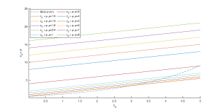
Figure 1: A comparison between the right-hand-side of (41) as a function of $c_{2}$ against several straight lines $c_{2}+\rho$ for different values of $\rho$, where the other parameters are fixed as $\beta=\gamma=1$, $\alpha=0.5.$ The right-hand-side of (41) is described using a dashed line(- - -). Target system (22)-(25) is exponentially stable for values of $c_{2}$ at which the straight line $c_{2}+\rho$, for some $\rho$, is above the dashed line(- - -). The figure showcases the restrictive nature associated with condition (41). The parameter $\rho$ has to be large or the coupling factor $\alpha\beta$ has to be small allowing for the inequality (41) to be fulfilled.

3.1 Numerical simulations

The solutions of system (1)-(4), both controlled and uncontrolled, were simulated numerically using a finite-element approximation in COMSOL Multiphysic software. The finite-element method (FEM) with linear splines was used to approximate the coupled equations by a system of DAEs. The spatial interval was divided into $27$ subintervals. Also, time was discretized by a time-stepping algorithm called generalized alpha with time-step= 0.2. We set $\gamma=\frac{1}{4}$, $\rho=\frac{1}{3}$, $\alpha=\frac{1}{4}$ and $\beta=\frac{1}{2}.$ For these parameter values, the system is unstable. Figure2 presents the dynamics of the states $w(x,t)$ and $v(x,t)$ in the absence of the control with initial condition $w(0)=\sin(\pi x).$ The system was first controlled with the controller resulting from the choice of parameter $c_{2}=1.2-\rho$ which satisfies inequality (41) and thus stability of the controlled system is guaranteed. This is illustrated in Figure2. As predicted by the theory, the dynamics of the system decay to zero with time. A comparison between the $L_{2}$-norm of both states $w(x,t)$ and $v(x,t)$ before and after applying the control input is given in Figure 3.

Comparison of open-loop and closed loop dynamics

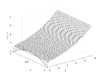
(a) uncontrolled $w(x,t)$

(b) uncontrolled $v(x,t)$

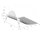
(c) controlled $w(x,t)$

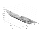
(d) controlled $v(x,t)$

Figure 2: A 3D landscape of the dynamics of a coupled parabolic-elliptic system (1)-(4) with initial condition $w_{0}=\sin(\pi x)$, without and with control. The parameters of the system are $\gamma=\frac{1}{4}$, $\rho=\frac{1}{3}$, $\alpha=\frac{1}{4}$ , $\beta=\frac{1}{2}.$ The uncontrolled system is unstable with this choice of parameters. The backstepping state-feedback control gain is $c_{2}=1.2-\rho$ which meets the stability condition (41). The control causes the solutions of the system to decay to the steady-state solution as $t\to\infty$.

Comparison of open-loop and closed-loop $L_{2}$-norms

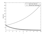
(a) $L_{2}$-norm $w(x,t)$

(b) $L_{2}$-norm $v(x,t)$

Figure 3: A comparison between the $L_{2}$-norm of the solutions $w(x,t)$ and $v(x,t)$ for the uncontrolled and controlled systems with initial condition $w_{0}=\sin(\pi x).$ The system parameters are $\gamma=\frac{1}{4}$, $\rho=\frac{1}{3}$, $\alpha=\frac{1}{4}$, $\beta=\frac{1}{2}$ so the uncontrolled system is unstable. In the absence of control, the $L_{2}$-norm of the states grows. The backstepping state-feedback control gain is given by $c_{2}=1.2-\rho;$ stability condition (41) is satisfied. The $L_{2}$-norm of the solution of the controlled system decays to zero.

4 Observer design

In the previous section, the control input was designed based on the assumption that the state of system (1)-(4) is known. The focus of this section is to design an observer that estimates the state of the parabolic-elliptic system.

We first design an observer using two measurements $v(1,t)$, and $w(1,t)$. As for the situation when two controls can be used, the design is fairly straightforward. The situation becomes more intricate with only one measurement is available. Then, as for the single control situation covered in the previous section, a bound must be satisfied.

4.1 Both $w(1,t)$ and $v(1,t)$ are available

The objective is to design an observer when the available measurements of system (1)-(4) are $w(1,t)$ and $v(1,t)$. We propose the following observer for system (1)-(4)

$$\hat{w}_{t}(x,t)= \hat{w}_{xx}(x,t)-\rho\hat{w}(x,t)+\alpha\hat{v}(x,t)$$

$$+\eta_{1}(x)[w(1,t)-\hat{w}(1,t)],$$ (42a)

$$0= \hat{v}_{xx}(x,t)-\gamma\hat{v}(x,t)+\beta\hat{w}(x,t)$$

$$+\eta_{2}(x)[v(1,t)-\hat{v}(1,t)],$$ (42b)

$$\hat{w}_{x}(0,t)= 0,\quad\hat{w}_{x}(1,t)=u(t)+\eta_{3}[w(1,t)-\hat{w}(1,t)],$$ (42c)

$$\hat{v}_{x}(0,t)= 0,\quad\hat{v}_{x}(1,t)=\eta_{4}[v(1,t)-\hat{v}(1,t)],$$ (42d)

Two in-domain output injection functions $\eta_{1}(x)$ and $\eta_{2}(x)$, and two boundary injections values $\eta_{3}$ and $\eta_{4}$ are to be designed. We will need the following lemma.

Lemma 11.

[25] The hyperbolic partial differential equation

$$k^{b}_{xx}(x,y)-k^{b}_{yy}(x,y)+o_{2}k^{b}(x,y)=0,\quad 0<x<y<1$$ (43a)

$$k^{b}_{x}(0,y)=0,\quad k^{b}(x,x)=-\frac{1}{2}o_{2}x,$$ (43b)

has a continuous unique solution. Here $o_{2}=o_{1}-\rho$, and $o_{2}>0$.

Define the error states

$$e^{w}(x,t)=w(x,t)-\hat{w}(x,t),$$ (44a)

$$e^{v}(x,t)=v(x,t)-\hat{v}(x,t).$$ (44b)

The observer error dynamics satisfy

$$e^{w}_{t}(x,t)= e^{w}_{xx}(x,t)-\rho e^{w}(x,t)+\alpha e^{v}(x,t)$$

$$-\eta_{1}(x)e^{w}(1,t),$$ (45a)

$$0= e^{v}_{xx}(x,t)-\gamma e^{v}(x,t)+\beta e^{w}(x,t)$$

$$-\eta_{2}(x)e^{v}(1,t),$$ (45b)

$$e^{w}_{x}(0,t)= 0,\quad e^{w}_{x}(1,t)=-\eta_{3}e^{w}(1,t),$$ (45c)

$$e^{v}_{x}(0,t)= 0,\quad e^{v}_{x}(1,t)=-\eta_{4}e^{v}(1,t),$$ (45d)

A backstepping approach is used to select $\eta_{1}(x),\;\eta_{2}(x),$ $\eta_{3},\;\eta_{4}$ so that the error system (45d) is exponentially stable. We introduce the target system

$$e^{\tilde{w}}_{t}(x,t)= e^{\tilde{w}}_{xx}(x,t)-(o_{2}+\rho)e^{\tilde{w}}(x,t)+\alpha e^{\tilde{v}}(x,t),$$ (46a)

$$0= e^{\tilde{v}}_{xx}(x,t)-(o_{2}+\gamma)e^{\tilde{v}}(x,t)+\beta e^{\tilde{w}}(x,t),$$ (46b)

$$e^{\tilde{w}}_{x}(0,t)= 0,\qquad e^{\tilde{w}}_{x}(1,t)=0,$$ (46c)

$$e^{\tilde{v}}_{x}(0,t)= 0,\qquad e^{\tilde{v}}_{x}(1,t)=0.$$ (46d)

A pair of state transformations

$$e^{w}(x,t)= e^{\tilde{w}}(x,t)-\int_{x}^{1}k_{1}(x,y)e^{\tilde{w}}(y,t)dy,$$ (47a)

$$e^{v}(x,t)= e^{\tilde{v}}(x,t)-\int_{x}^{1}k_{2}(x,y)e^{\tilde{v}}(y,t)dy,$$ (47b)

that transform the target system (46) into (45) are needed.

Theorem 12.

If $k_{1}(x,y)=k_{2}(x,y)=k^{b}(x,y)$ where $k^{b}(x,y)$ satisfies (43), and if the output injections are

$$\eta_{1}(x)=\eta_{2}(x)=-k^{b}_{y}(x,1),$$ (48)

$$\eta_{3}=\eta_{4}=-k^{b}(1,1),$$ (49)

then transformations (47a) and (47b) convert the target system (46) into the original error dynamics (45).

Proof. We first take the spatial derivatives of (47a).

$$e_{x}^{w}(x,t)=e^{\tilde{w}}_{x}(x,t)-\int_{x}^{1}k_{1x}(x,y)e^{\tilde{w}}(y,t)dy$$

$$+k_{1}(x,x)e^{\tilde{w}}(x,t)$$ (50)

$$e^{w}_{xx}(x,t)=e^{\tilde{w}}_{xx}(x,t)-\int_{x}^{1}k_{1xx}(x,y)e^{\tilde{w}}(y,t)dy$$

$$+k_{1x}(x,x)e^{\tilde{w}}(x,t)+\frac{d}{dx}k_{1}(x,x)e^{\tilde{w}}(x,t)$$

$$+k_{1}(x,x)e^{\tilde{w}}_{x}(x,t).\hfill$$ (51)

Taking the time derivative of (47a) and integrating by parts

$$e^{w}_{t}(x,t)=e^{\tilde{w}}_{t}(x,t)-\int_{x}^{1}k_{1}(x,y)e^{\tilde{w}}_{t}(y,t)dy$$

$$=e^{\tilde{w}}_{t}(x,t)+(o_{2}+\rho)\int_{x}^{1}k_{1}(x,y)e^{\tilde{w}}(y,t)dy-k_{1}(x,1)$$

$$\times e^{\tilde{w}}_{x}(1,t)-\alpha\int_{x}^{1}k_{1}(x,y)e^{\tilde{v}}(y,t)dy+k_{1}(x,x)e^{\tilde{w}}_{x}(x,t)$$

$$+k_{1y}(x,1)e^{\tilde{w}}(1,t)-k_{1y}(x,x)e^{\tilde{w}}(x,t)$$

$$-\int_{x}^{1}k_{1yy}(x,y)e^{\tilde{w}}(y,t)dy.$$ (52)

We rewrite the right-hand-side of the parabolic equation (45a) of the error dynamics as

$$e^{w}_{t}(x,t)-e^{w}_{xx}(x,t)+\rho e^{w}(x,t)-\alpha e^{v}(x,t)$$

$$+\eta_{1}(x)e^{w}(1,t)=0.$$ (53)

Substituting (51) and (52) in (53), then the left-hand-side of (53) is

$$\text{(L.H.S)}_{1}=e^{\tilde{w}}_{t}(x,t)-e^{\tilde{w}}_{xx}(x,t)-\int_{x}^{1}k_{1yy}(x,y)$$

$$\times e^{\tilde{w}}(y,t)dy+(o_{2}+\rho)\int_{x}^{1}k_{1}(x,y)e^{\tilde{w}}(y,t)dy$$

$$+\int_{x}^{1}k_{1xx}(x,y)e^{\tilde{w}}(y,t)dy-k_{1y}(x,x)e^{\tilde{w}}(x,t)$$

$$-k_{1x}(x,x)e^{\tilde{w}}(x,t)-\frac{d}{dx}k_{1}(x,x)e^{\tilde{w}}(x,t)-k_{1}(x,x)$$

$$\times e^{\tilde{w}}_{x}(x,t)+k_{1}(x,x)e^{\tilde{w}}_{x}(x,t)+\rho e^{\tilde{w}}(x,t)-\alpha e^{\tilde{v}}(x,t)$$

$$-\rho\int_{x}^{1}k_{1}(x,y)e^{\tilde{w}}(y)dy+\eta_{1}(x)e^{\tilde{w}}(1,t)+k_{1y}(x,1)$$

$$\times e^{\tilde{w}}(1,t)-k_{1}(x,1)e^{\tilde{w}}_{x}(1,t)-\alpha\int_{x}^{1}k_{1}(x,y)e^{\tilde{v}}(y,t)dy$$

$$+\alpha\int_{x}^{1}k_{2}(x,y)e^{\tilde{v}}(y,t)dy,$$ (54)

$$\text{(R.H.S)}_{1}=0.$$ (55)

Adding and subtracting the term $(o_{2}+\rho)e^{\tilde{w}}(x,t)$ to the right-hand-side of (54)

$$\text{(L.H.S)}_{1}=e^{\tilde{w}}_{t}(x,t)-e^{\tilde{w}}_{xx}(x,t)+o_{2}e^{\tilde{w}}(x,t)-\alpha e^{\tilde{v}}(x,t)$$

$$-\int_{x}^{1}[-o_{2}k_{1}(x,y)-k_{1xx}(x,y)+k_{1yy}(x,y)]e^{\tilde{w}}(y,t)dy$$

$$-k_{1}(x,1)e^{\tilde{w}}_{x}(1,t)-(2\frac{d}{dx}k(x,x)+o_{2})e^{\tilde{w}}(x,t)$$

$$+(\eta_{1}(x)+k_{1y}(x,1))e^{\tilde{w}}(1,t)-\alpha\int_{x}^{1}k_{1}(x,y)e^{\tilde{v}}(y,t)dy$$

$$+\alpha\int_{x}^{1}k_{2}(x,y)e^{\tilde{v}}(y,t)dy.$$ (56)

Using the boundary condition $e^{\tilde{w}}_{x}(1,t)=0$, if $k_{1}(x,y)=k_{2}(x,y)=k^{b}(x,y)$ then equation (56) reduces to

$$\text{(L.H.S)}_{1}=e^{\tilde{w}}_{t}(x,t)-e^{\tilde{w}}_{xx}(x,t)+(o_{2}+\gamma)e^{\tilde{w}}(x,t)$$

$$-\alpha e^{\tilde{v}}(x,t)-\int_{x}^{1}[-o_{2}k^{b}(x,y)-k^{b}_{xx}(x,y)+k^{b}_{yy}(x,y)]$$

$$\times e^{\tilde{w}}(y,t)dy-(2\frac{d}{dx}k^{b}(x,x)+o_{2})e^{\tilde{w}}(x,t)$$

$$+(\eta_{1}(x)+k^{b}_{y}(x,1))e^{\tilde{w}}(1,t).$$ (57)

If $k^{b}(x,y)$ satisfies (43) and $\eta_{1}(x)=k^{b}_{y}(x,1)$, then (57) becomes

$$\text{(L.H.S)}_{1}=e^{\tilde{w}}_{t}(x,t)-e^{\tilde{w}}_{xx}(x,t)+(o_{2}+\gamma)e^{\tilde{w}}(x,t)$$

$$-\alpha e^{\tilde{v}}(x,t).$$

Referring to (55) and (46a),

$$\text{(L.H.S)}_{1}=0=\text{(R.H.S)}_{1}.$$

Hence the state transformation (47) transforms the parabolic equation (46a) into (45a). Referring to (50), we apply transformation (47a) to the boundary conditions (46c)

$$e_{x}^{w}(0,t)= e^{\tilde{w}}_{x}(0,t)-\int_{0}^{1}k^{b}_{x}(0,y)e^{\tilde{w}}(y,t)dy$$

$$+k^{b}(0,0)e^{\tilde{w}}(0,t)$$

$$= 0,$$

where the previous step was obtained by using (43b) and $e^{\tilde{w}}(0,t)=e^{w}(0,t)$. Thus we obtain the boundary condition in (45c) at $x=0$. Similarly,

$$e_{x}^{w}(1,t)= e^{\tilde{w}}_{x}(1,t)-\int_{1}^{1}k^{b}_{x}(1,y)e^{\tilde{w}}(y,t)dy$$

$$+k^{b}(1,1)e^{\tilde{w}}(1,t)$$

$$= k^{b}(1,1)e^{\tilde{w}}(1,t)=k^{b}(1,1)e^{w}(1,t).$$

If $\eta_{3}=-k^{b}(1,1)$ then we obtain the boundary condition in (45c) at $x=1$. We perform similar calculations on the elliptic equation (46c). First, we take the spatial derivative of (47b),

$$e^{v}_{xx}(x,t)=e^{\tilde{v}}_{xx}(x,t)-\int_{x}^{1}k_{2xx}(x,y)e^{\tilde{v}}(y,t)dy$$

$$+k_{2x}(x,x)e^{\tilde{v}}(x,t)+\frac{d}{dx}k_{2}(x,x)e^{\tilde{v}}(x,t)$$

$$+k_{2}(x,x)e^{\tilde{v}}_{x}(x,t).$$ (58)

Subbing (58) in the right-hand-side of elliptic equation (45b),

$$\text{(R.H.S)}_{2}=e^{\tilde{v}}_{xx}(x,t)-\int_{x}^{1}k_{2xx}(x,y)e^{\tilde{v}}(y,t)dy$$

$$+k_{2x}(x,x)e^{\tilde{v}}(x,t)+\frac{d}{dx}k_{2}(x,x)e^{\tilde{v}}(x,t)+k_{2}(x,x)$$

$$\times e^{\tilde{v}}_{x}(x,t)-\gamma e^{\tilde{v}}(x,t)+\gamma\int_{x}^{1}k_{2}(x,y)e^{\tilde{v}}(y,t)dy$$

$$+\beta e^{\tilde{w}}(x,t)-\beta\int_{x}^{1}k_{1}(x,y)e^{\tilde{w}}(y,t)dy-\eta_{2}(x)e^{\tilde{v}}(1,t)$$ (59)

$$\text{(L.H.S)}_{2}=0.$$ (60)

Rewriting the last term of (59) as follows

$$\beta\int_{x}^{1}k_{1}(x,y)e^{\tilde{w}}(y,t)dy=-\int_{x}^{1}k_{1}(x,y)e^{\tilde{v}}_{yy}(y,t)dy$$

$$+(o_{2}+\gamma)\int_{x}^{1}k_{1}(x,y)e^{\tilde{v}}(y,t)dy,$$

which can be obtained by referring to the elliptic equation of (46b), then (59) gives

$$\text{(R.H.S)}_{2}=e^{\tilde{v}}_{xx}(x,t)-\int_{x}^{1}k_{2xx}(x,y)e^{\tilde{v}}(y,t)dy$$

$$+k_{2x}(x,x)e^{\tilde{v}}(x,t)+\frac{d}{dx}k_{2}(x,x)e^{\tilde{v}}(x,t)+k_{2}(x,x)$$

$$\times e^{\tilde{v}}_{x}(x,t)-\gamma e^{\tilde{v}}(x,t)+\gamma\int_{x}^{1}k_{2}(x,y)e^{\tilde{v}}(y,t)dy$$

$$+\beta e^{\tilde{w}}(x,t)+\int_{x}^{1}k_{1}(x,y)e^{\tilde{v}}_{yy}(y,t)dy-\eta_{2}(x)e^{\tilde{v}}(1,t)$$

$$-(o_{2}+\gamma)\int_{x}^{1}k_{1}(x,y)e^{\tilde{v}}(y,t)dy.$$ (61)

Since $k_{1}(x,y)=k_{2}(x,y)=k^{b}(x,y)$ , then (61) leads to

$$\text{(R.H.S)}_{2}=e^{\tilde{v}}_{xx}(x,t)-\int_{x}^{1}k^{b}_{xx}(x,y)e^{\tilde{v}}(y,t)dy$$

$$+k^{b}_{x}(x,x)e^{\tilde{v}}(x,t)+\frac{d}{dx}k^{b}(x,x)e^{\tilde{v}}(x,t)+k^{b}(x,x)$$

$$\times e^{\tilde{v}}_{x}(x,t)-\gamma e^{\tilde{v}}(x,t)+\gamma\int_{x}^{1}k^{b}(x,y)e^{\tilde{v}}(y,t)dy$$

$$+\beta e^{\tilde{w}}(x,t)-(o_{2}+\gamma)\int_{x}^{1}k^{b}(x,y)e^{\tilde{v}}(y,t)dy-\eta_{2}(x)$$

$$\times e^{\tilde{v}}(1,t)+e^{\tilde{v}}_{x}(1,t)k^{b}(x,1)-e^{\tilde{v}}_{x}(x,t)k^{b}(x,x)-e^{\tilde{v}}(1,t)$$

$$\times k^{b}_{y}(x,1)+e^{\tilde{v}}(x,t)k^{b}_{y}(x,x)+\int_{x}^{1}k^{b}_{yy}(x,y)e^{\tilde{v}}(y,t)dy.$$

Adding and subtracting the term $o_{2}e^{\tilde{v}}(x,t)$ and incorporating $e^{\tilde{v}}_{x}(1,t)=0$,

$$\text{(R.H.S)}_{2}=e^{\tilde{v}}_{xx}(x,t)-(o_{2}+\gamma)e^{\tilde{v}}(x,t)+\beta e^{\tilde{w}}(x,t)$$

$$+\int_{x}^{1}[-k_{xx}(x,y)+k_{yy}(x,y)-o_{2}k(x,y)]e^{\tilde{v}}(y,t)dy$$

$$+(2\frac{d}{dx}k^{b}(x,x)+o_{2})e^{\tilde{v}}(x,t)-(k^{b}_{y}(x,1)+\eta_{2}(x))$$

$$\times e^{\tilde{v}}(1,t).$$ (62)

Since $k^{b}(x,y)$ is given by (43) and $\eta_{2}(x)=-k^{b}_{y}(x,1)$, then referring to (46b) and (60)

$$\text{(L.H.S)}_{2}=0=\text{(R.H.S)}_{2}.$$

Thus the state transformation (47) transforms the elliptic equation (46b) into (45b). We apply the transformation to the boundary conditions (46d),

$$e_{x}^{v}(0,t)= e^{\tilde{v}}_{x}(0,t)-\int_{0}^{1}k^{b}_{x}(0,y)e^{\tilde{v}}(y,t)dy$$

$$+k^{b}(0,0)e^{\tilde{v}}(0,t)=0,$$

by means of using (43b) and that $e^{\tilde{v}}_{x}(0,t)=0$ . We obtain the boundary condition at $x=0$ in (45d). Similarly,

$$e_{x}^{v}(1,t)= e^{\tilde{v}}_{x}(1,t)-\int_{1}^{1}k^{b}_{x}(1,y)e^{\tilde{v}}(y,t)dy+k^{b}(1,1)$$

$$e^{\tilde{v}}(1,t)$$

$$= k^{b}(1,1)e^{\tilde{v}}(1,t)=k^{b}(1,1)e^{v}(1,t),$$

where the previous step was obtained by noting that $e^{\tilde{v}}(0,t)=e^{v}(0,t)$. If $\eta_{4}=-k^{b}(1,1)$ then we obtain the second boundary condition in (45d) at $x=1$. The conclusion of the theorem follows. $\hfill\square$

The next theorem follows from Theorem 12.

Theorem 13.

Let $k(x,y)$ be the solution of system (43). The error dynamics (45) with output injections $\eta_{j},\;j=1,\dots,4$ defined as given in (48)-(49) are exponentially stable if and only if the parameter $o_{2}$ satisfies

$$(o_{2}+\rho)(o_{2}+\gamma)>\alpha\beta,$$ (63)

and $o_{2}+\gamma\neq-(n\pi)^{2}$.

Proof. If $o_{2}$ is given by (63) such that $o_{2}+\gamma\neq-(n\pi)^{2}$, the target system (46) has a unique solution and is exponentially stable due to the criteria for stability of parabolic-elliptic systems established previously in Corollary 2 (of a previous draft). Finally, the exponential stability of the error dynamics (45) follows by referring to Theorem 12 and using the invertiblity of transformation (47). This concludes the proof. $\hfill\square$

4.2 Only $w(1,t)$ is available

The objective of this subsection is to design an exponentially convergent observer for (1)-(4) given only a single measurement $w(1,t)$. We propose the following observer

$$\hat{w}_{t}(x,t)= \hat{w}_{xx}(x,t)-\rho\hat{w}(x,t)+\alpha\hat{v}(x,t)$$

$$+\eta_{1}(x)[w(1,t)-\hat{w}(1,t)],$$ (64a)

$$0= \hat{v}_{xx}(x,t)-\gamma\hat{v}(x,t)+\beta\hat{w}(x,t),$$ (64b)

$$\hat{w}_{x}(0,t)= 0,\quad\hat{w}_{x}(1,t)=u(t)+\eta_{2}[w(1,t)-\hat{w}(1,t)],$$ (64c)

$$\hat{v}_{x}(0,t)= 0,\quad\hat{v}_{x}(1,t)=0,$$ (64d)

where $\eta_{1}(x)$ and $\eta_{2}$ are output injections to be designed. Defining the states of the error dynamics as in (44), the system describing the observation error satisfies

$$e^{w}_{t}(x,t)= e^{w}_{xx}(x,t)-\rho e^{w}(x,t)+\alpha e^{v}(x,t)$$

$$-\eta_{1}(x)e^{w}(1,t),$$ (65a)

$$0= e^{v}_{xx}(x,t)-\gamma e^{v}(x,t)+\beta e^{w}(x,t),$$ (65b)

$$e^{w}_{x}(0,t)= 0,\quad e^{w}_{x}(1,t)=-\eta_{2}e^{w}(1,t),$$ (65c)

$$e^{v}_{x}(0,t)= 0,\quad e^{v}_{x}(1,t)=0.$$ (65d)

Both of $\eta_{1}(x)$ and $\eta_{2}$ have to be chosen so that exponential stability of error dynamics is achieved. Following a backstepping approach, we define the transformation

$$e^{\tilde{w}}(x,t)=e^{w}(x,t)-\int_{0}^{x}k^{a}(x,y)e^{w}(y,t)dy,$$ (66)

where $k^{a}(x,y)$ is given by (16) with $c_{2}$ replaced by $o_{2}$. The inverse transformation [16, Chap. 4, section 5] is

$$e^{w}(x,t)=e^{\tilde{w}}(x,t)+\int_{0}^{x}\ell^{a}(x,y)e^{\tilde{w}}(y,t)dy,$$ (67)

where $\ell^{a}$ satisfies system (19).

Theorem 14.

If the output injections are

$$\eta_{1}(x)=0,$$ (68)

$$\eta_{2}=-k^{a}(1,1),$$ (69)

where $k^{a}(x,y)$ is given in (16) with $c_{2}$ being replaced by $o_{2}$ then transformation (71) converts the error dynamics (65) into the target system

$$e^{\tilde{w}}_{t}(x,t)=e^{\tilde{w}}_{xx}(x,t)-(o_{2}+\rho)e^{\tilde{w}}(x,t)+\alpha e^{v}(x,t)$$

$$-\alpha\int_{0}^{x}k^{a}(x,y)e^{v}(y,t)dy,$$ (70a)

$$0=e^{v}_{xx}(x,t)-\gamma e^{v}(x,t)+\beta e^{\tilde{w}}(x,t)$$

$$+\beta\int_{0}^{x}\ell^{a}(x,y)e^{\tilde{w}}(y,t)dy,$$ (70b)

$$e^{\tilde{w}}_{x}(1,t)=-\int_{0}^{1}k^{a}_{x}(1,y)e^{\tilde{w}}(y,t)dy$$

$$-\int_{0}^{1}k^{a}_{x}(1,y)\int_{0}^{y}\ell^{a}(y,z)e^{\tilde{w}}(z,t)dzdy,$$ (70c)

$$e^{\tilde{w}}_{x}(0,t)=0,\quad e^{v}_{x}(0,t)=0,\quad e^{v}_{x}(1,t)=0.$$ (70d)

Proof. It will be useful to rewrite (66) as

$$e^{w}(x,t)=e^{\tilde{w}}(x,t)+\int_{0}^{x}k^{a}(x,y)e^{w}(y,t)dy.$$ (71)

We take the spatial and the time derivatives of (71) we have

$$e^{w}_{xx}(x,t)=e^{\tilde{w}}_{xx}(x,t)+\int_{0}^{x}k^{a}_{xx}(x,y)e^{w}(y,t)dy$$

$$+k^{a}_{x}(x,x)e^{w}(x,t)+\frac{d}{dx}k^{a}(x,x)e^{w}(x,t)$$

$$+k^{a}(x,x)e^{w}_{x}(x,t),$$ (72)

$$e^{w}_{t}(x,t)=e^{\tilde{w}}_{t}(x,t)+\int_{0}^{x}k^{a}(x,y)e^{w}_{t}(y,t)dy$$

$$=e^{\tilde{w}}_{t}(x,t)-\rho\int_{0}^{x}k^{a}(x,y)e^{w}(y,t)dy+\alpha\int_{0}^{x}k^{a}(x,y)$$

$$\times e^{v}(y,t)dy+k^{a}(x,x)e^{w}_{x}(x,t)-k^{a}(x,0)e^{w}_{x}(0,t)$$

$$-k^{a}_{y}(x,x)e^{w}(x,t)+k^{a}_{y}(x,0)e^{w}(0,t)+\int_{0}^{x}k^{a}_{yy}(x,y)$$

$$\times e^{w}(y,t)dy-e^{w}(1,t)\int_{0}^{x}k^{a}(x,y)\eta_{1}(y)dy.$$ (73)

Substituting (72) and (73) in the parabolic equation (65a), and using $e^{w}_{x}(0,t)=0$ and $k^{a}_{y}(x,0)=0$,

$$e^{w}_{t}(x,t)=e^{w}_{xx}(x,t)+\alpha e^{v}(x,t)+\left(k^{a}_{y}(x,x)+k^{a}_{x}(x,x)\right)$$

$$\times e^{w}(x,t)+\frac{d}{dx}k^{a}(x,x)e^{w}(x,t)-\rho e^{w}(x,t)+k^{a}(x,x)$$

$$\times e^{w}_{x}(x,t)-k^{a}(x,x)e^{w}_{x}(x,t)+\int_{0}^{x}[k^{a}_{xx}(x,y)$$

$$-k^{a}_{yy}(x,y)+\rho k^{a}(x,y)]e^{w}(y,t)dy-\alpha\int_{0}^{x}k^{a}(x,y)$$

$$\times e^{v}(y,t)dy+e^{w}(1,t)\int_{0}^{x}k^{a}(x,y)\eta_{1}(y)dy$$

$$-\eta_{1}(x)e^{w}(1,t).$$ (74)

Adding and subtracting the term $(o_{2}+\rho)e^{w}(x,t)$ to the right-hand-side of equation (74), and noting that $k^{a}(x,y)$ is given by (15),

$$e^{w}_{t}(x,t)=e^{w}_{xx}(x,t)-\rho e^{w}(x,t)+\alpha e^{v}(x,t)$$

$$-\alpha\int_{0}^{x}k^{a}(x,y)e^{v}(y,t)dy-e^{w}(1,t)\int_{0}^{x}k^{a}(x,y)$$

$$\times\eta_{1}(y)dy-\eta_{1}(x)e^{w}(1,t).$$

If $\eta_{1}(x)=0$, we obtain the parabolic equation (70a). We now apply transformation (71) on the boundary conditions (65c), using lemma 4

$$e^{\tilde{w}}_{x}(0,t) =e^{w}_{x}(0,t)-\int_{0}^{0}k^{a}_{x}(1,y)w(y)dy$$

$$-k^{a}(0,0)w(1,t)=0,$$

by virtue of referring to the boundary conditions of system (15).

$$e^{\tilde{w}}_{x}(1,t)=e^{w}_{x}(1,t)-\int_{0}^{1}k^{a}_{x}(1,y)e^{w}(y,t)dy$$

$$-k^{a}(1,1)e^{w}(1,t)$$

$$= -(\eta_{2}+k^{a}(1,1))e^{w}(1,t)-\int_{0}^{1}k^{a}_{x}(1,y)e^{w}(y,t)dy$$

$$= -\int_{0}^{1}k^{a}_{x}(1,y)e^{w}(y,t)dy.$$

$$= -\int_{0}^{1}k^{a}_{x}(1,y)e^{\tilde{w}}(y,t)dy-\int_{0}^{1}k^{a}_{x}(1,y)\int_{0}^{y}\ell^{a}(y,z)$$

$$\times e^{\tilde{w}}(z,t)dzdy.$$

The previous equation holds true via using (69) and using the inverse transformation (67). The elliptic equation (70b) can be obtained via using the inverse transformation (67). $\hfill\square$

Theorem 15.

The target system (70) is exponentially stable if $o_{2}$ is chosen such that

$$o_{2}+\rho >\frac{|\alpha||\beta|}{\gamma}(1+\|k^{a}\|)(1+\|\ell^{a}\|)$$

$$+\frac{(1+\|\ell^{a}\|)^{2}\|k^{a}_{x}(1,y)\|^{2}+2}{2}.$$ (75)

Proof. We define the Lyapunov function candidate,

$$V(t)= \frac{1}{2}\int_{0}^{1}(e^{\tilde{w}}(x,t))^{2}dx=\frac{1}{2}\|e^{\tilde{w}}(x,t)\|^{2}.$$

Taking the time derivative of $V(t)$,

$$\dot{V}(t)=\int_{0}^{1}e^{\tilde{w}}(x,t)e^{\tilde{w}}_{t}(x,t)dx$$

$$= \int_{0}^{1}e^{\tilde{w}}(x,t)e^{\tilde{w}}_{xx}(x,t)dx-(o_{2}+\rho)\int_{0}^{1}(e^{\tilde{w}}(x,t))^{2}dx$$

$$+\alpha\int_{0}^{1}e^{\tilde{w}}(x,t)e^{v}(x,t)dx-\alpha\int_{0}^{1}e^{\tilde{w}}(x,t)\int_{0}^{x}k^{a}(x,y)$$

$$\times e^{v}(y,t)dydx.$$ (76)

Integrating the term $\int_{0}^{1}e^{\tilde{w}}(x,t)e^{\tilde{w}}_{xx}(x,t)dx$ by parts, and using the boundary conditions (70c)-(70d)

$$\int_{0}^{1}e^{\tilde{w}}(x,t)e^{\tilde{w}}_{xx}(x,t)dx=e^{\tilde{w}}(1,t)e^{\tilde{w}}_{x}(1,t)$$

$$-e^{\tilde{w}}(0,t)e^{\tilde{w}}_{x}(0,t)-\|e^{\tilde{w}}_{x}\|^{2}$$

$$=e^{\tilde{w}}(1,t)e^{\tilde{w}}_{x}(1,t)-\|e^{\tilde{w}}_{x}\|^{2}$$

$$=-\int_{0}^{1}k^{a}_{x}(1,y)e^{w}(y,t)dy\,e^{\tilde{w}}(1,t)-\|e^{\tilde{w}}_{x}\|^{2}.$$ (77)

To bound the term $-\int_{0}^{1}k^{a}_{x}(1,y)e^{w}(y,t)dy\,e^{\tilde{w}}(1,t)$ in (77), we use Cauchy-Schwartz,

$$-\int_{0}^{1}k^{a}_{x}(1,y)e^{w}(y,t)dye^{\tilde{w}}(1,t)$$

$$\leq\|\int_{0}^{1}k^{a}_{x}(1,y)e^{w}(y,t)dy\|\max_{x\in[0,1]}e^{\tilde{w}}(x,t)$$

$$\leq\|k^{a}_{x}(1,y)\|\|e^{w}\|\|e^{\tilde{w}}\|_{\infty}.$$

Invoking Agmon’s inequality [29] on the right-hand-side of the previous inequality leads to

$$-\int_{0}^{1}k^{a}_{x}(1,y)e^{w}(y,t)dye^{\tilde{w}}(1,t)$$

$$\leq\|k^{a}_{x}(1,y)\|\|e^{w}\|\|e^{\tilde{w}}\|^{1/2}\|e^{\tilde{w}}\|_{H^{1}}^{1/2}.$$

Using Young’s inequality on the right-hand-side of the previous inequality,

$$-\int_{0}^{1}k^{a}_{x}(1,y)e^{w}(y,t)dye^{\tilde{w}}(1,t)$$

$$\leq\frac{\|k^{a}_{x}(1,y)\|^{2}}{2}\|e^{w}\|^{2}+\frac{1}{2}(\|e^{\tilde{w}}\|\|e^{\tilde{w}}\|_{H^{1}})$$

$$\leq\frac{\|k^{a}_{x}(1,y)\|^{2}}{2}\|e^{w}\|^{2}+\frac{1}{2}\|e^{\tilde{w}}\|^{2}+\frac{1}{2}\|e^{\tilde{w}}\|\|e^{\tilde{w}}_{x}\|.$$

Estimating the term $\frac{1}{2}\|e^{\tilde{w}}\|\|e^{\tilde{w}}_{x}\|$ on the right-hand-side of the previous inequality using Young’s inequality, then

$$-\int_{0}^{1}k^{a}_{x}(1,y)e^{w}(y,t)dye^{\tilde{w}}(1,t)\leq\frac{\|k^{a}_{x}(1,y)\|^{2}}{2}\|e^{w}\|^{2}$$

$$+\|e^{\tilde{w}}\|^{2}+\frac{1}{4}\|e^{\tilde{w}}_{x}\|^{2}.$$ (78)

Referring to the inverse transformation (67),

$$-\int_{0}^{1}k^{a}_{x}(1,y)e^{w}(y,t)dye^{\tilde{w}}(1,t)$$

$$\leq\frac{(1+\|\ell^{a}\|)^{2}\|k^{a}_{x}(1,y)\|^{2}+2}{2}\|e^{\tilde{w}}\|^{2}+\frac{1}{4}\|e^{\tilde{w}}_{x}\|^{2}.$$ (79)

Combining (79) and (77), we get

$$\int_{0}^{1}e^{\tilde{w}}(x,t)e^{\tilde{w}}_{xx}(x,t)dx$$

$$\leq\frac{(1+\|\ell^{a}\|)^{2}\|k^{a}_{x}(1,y)\|^{2}+2}{2}\|e^{\tilde{w}}\|^{2}-(1-\frac{1}{2})\|e^{\tilde{w}}_{x}\|^{2}$$

$$\leq\frac{(1+\|\ell^{a}\|)^{2}\|k^{a}_{x}(1,y)\|^{2}+2}{2}\|e^{\tilde{w}}\|^{2}.$$ (80)

Bounding the terms on the right-hand side of (76) using (80), Cauchy-Schwartz inequality and lemma 8, we arrive to

$$\dot{V}(t)\leq -(o_{2}+\rho-\frac{|\alpha||\beta|}{\gamma}(1+\|k^{a}\|)(1+\|\ell^{a}\|)$$

$$-\frac{(1+\|\ell^{a}\|)^{2}\|k^{a}_{x}(1,y)\|^{2}+2}{2})\|e^{\tilde{w}}\|^{2}.$$ (81)

Setting

$$o_{3}= o_{2}+\rho-\frac{|\alpha||\beta|}{\gamma}(1+\|k^{a}\|)(1+\|\ell^{a}\|)$$

$$-\frac{(1+\|\ell^{a}\|)^{2}\|k^{a}_{x}(1,y)\|^{2}+2}{2},$$

then inequality (81) implies that $V(t)\leq e^{-2o_{3}t}V(0)$. If the parameter $o_{2}$ is chosen such that (75) is satisfied, then $V(t)$ decays exponentially as $t\rightarrow\infty$. Thus, $\|e^{\tilde{w}}(x,t)\|$ decays exponentially. Referring to the elliptic equation of system (65) and recalling lemma 8, the state $e^{v}(x,t)$ is asymptotically stable. Exponential stability of system (70) follows by noting that $\partial_{xx}-\gamma I$ is boundedly invertible, and using a similar argument as the one given in the last part in the proof of Theorem 9. $\hfill\square$

The following lemma, which establishes a bound on $\|k^{a}_{x}(1,y)\|$, will be needed.

Lemma 16.

Consider system (15) with $c_{2}$ being replaced by $o_{2}$. The $L^{2}$-norm of $k^{a}_{x}(1,y)$ is bounded by

$$\|k^{a}_{x}(1,y)\|\leq\frac{o_{2}}{2}(1+\frac{o_{2}}{2})e^{\frac{o_{2}}{4}}\left(\sqrt{\frac{\pi}{2o_{2}}}erf(\sqrt{\frac{o_{2}}{2}})\right)^{\frac{1}{2}}.$$ (82)

Proof. The relation (82) can be shown by noting that the solution of system (15) is

$$k^{a}(x,y)=-o_{2}x\frac{I_{1}(\sqrt{o_{2}(x^{2}-y^{2})})}{\sqrt{o_{2}(x^{2}-y^{2})}}.$$

After straightforward mathematical steps, we arrive to

$$k^{a}_{x}(x,y)= -o_{2}\frac{I_{1}(\sqrt{o_{2}(x^{2}-y^{2})})}{\sqrt{o_{2}(x^{2}-y^{2})}}$$

$$-o_{2}x\frac{I_{2}(\sqrt{o_{2}(x^{2}-y^{2})}}{(x^{2}-y^{2})},$$ (83)

where we have used that $\frac{d}{dx}I_{1}(x)=\frac{I_{1}(x)}{x}+I_{2}(x)$. Setting $z=\sqrt{o_{2}(x^{2}-y^{2})}$ and using the definition of Bessel function, (83) can be written as

$$k^{a}_{x}(x,y)=-o_{2}\frac{I_{1}(z)}{z}-o_{2}^{2}x\frac{I_{2}(z)}{z^{2}}$$

$$=-\frac{o_{2}}{z}\sum_{m=0}^{\infty}\left(\frac{z}{2}\right)^{2m+1}\frac{1}{m!m+1!}-\frac{o_{2}^{2}}{z^{2}}x\sum_{m=0}^{\infty}\left(\frac{z}{2}\right)^{2m+2}$$

$$\times\frac{1}{m!m+2!}.$$ (84)

To find a bound on the induced $L_{2}$- norm of $k^{a}_{x}(1,y)$, with $x=1$ the variable $z$ becomes $z=\sqrt{o_{2}(1-y^{2})}$ where $0<y<1$. Equation (84) leads to

$$\|k^{a}_{x}(1,y)\|\leq\frac{o_{2}}{2}\sum_{m=0}^{\infty}\frac{(z^{2}/4)^{m}}{m!}+\frac{o_{2}^{2}}{4}x\sum_{m=0}^{\infty}\frac{(z^{2}/4)^{m}}{m!}$$

$$\leq\frac{o_{2}}{2}\|e^{\frac{z^{2}}{4}}\|+\frac{o_{2}^{2}}{4}\|e^{\frac{z^{2}}{4}}\|=\frac{o_{2}}{2}(1+\frac{o_{2}}{2})\|e^{\frac{z^{2}}{4}}\|$$

$$\leq\frac{o_{2}}{2}(1+\frac{o_{2}}{2})e^{\frac{o_{2}}{4}}\|e^{\frac{-o_{2}y^{2}}{4}}\|.$$ (85)

Since $\;erf(x)=\frac{2}{\sqrt{\pi}}\int_{0}^{x}e^{-\xi^{2}}d\xi$, inequality (85) leads to (82). $\square$

Using lemma 7 and lemma 16, the next corollary to Theorem 15 is now immediate.

Corollary 17.

The observation error dynamics (70) is exponentially stable if

$$o_{2}+\rho>\left(\frac{|\alpha||\beta|}{\gamma}+\frac{\|k^{a}_{x}(1,y)\|^{2}}{2}\right)$$

$$\times\left[1+\sqrt{\frac{o_{2}\pi}{2}}\;\left(erfi(\sqrt{\frac{o_{2}}{2}})\right)^{\frac{1}{2}}\left(erf(\sqrt{\frac{o_{2}}{2}})\right)^{\frac{1}{2}}\right]^{2}+1.$$ (86)

The following result now follows from Theorem 14 and Theorem 15.

Theorem 18.

Let $k^{a}(x,y)$ be the solution of system (15). The error dynamics (65) with output injection $\eta_{2}=\frac{1}{2}o_{2}$ defined as given in (69) are exponentially stable if $o_{2}$ is given by (75).

Condition (86) for stability of the observation error dynamics, imposes restrictions on the permissible choices of system parameters. This observation is demonstrated in Figure4, where we present a comparison between the right-hand-side of inequality (86) as a function of $o_{2}$, and several straight lines $o_{2}+\rho$ varying with different $\rho$. The other parameters are fixed as $\beta=\gamma=1,\;\alpha=0.5$. The dashed line in 4 represents the right-hand-side of (86). The observation error dynamics (65) is exponentially stable if the values of $o_{2}$ are such that the dashed line in Figure4 is beneath the straight lines, for different $\rho$.

Illustration of the restriction (86) on $o_{2}$

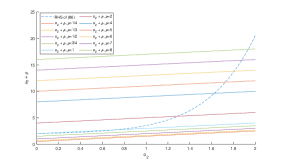
Figure 4: A comparison between the right-hand-side of inequality (86) as a function of $o_{2}$ against several straight lines $o_{2}+\rho$ for different values of $\rho$, while the other parameters are fixed as $\beta=\gamma=1$, $\alpha=0.5$. The right-hand-side of (86) is described using a dashed line(- - -). For any $\rho$, the error dynamics (70) is exponentially stable if $o_{2}$ is such that the dashed line(- - -) is beneath the straight line $o_{2}+\rho$. This illustrates the constraints associated with condition (86).

4.3 Numerical simulations

We conducted numerical simulations for the dynamics of both the coupled system (1)-(4) and the state observer (42) in the situation where two measurements, $w(1,t)$ and $v(1,t),$ are available. The simulations were performed using COMSOL Multiphysic software using linear splines to approximate the coupled equations by a system of DAEs. The spatial interval was divided into $27$ subintervals. Time was discretized by a time-stepping algorithm called generalized alpha with time-step= 0.1.

Observer designs were done for system (1)-(4) with $u(t)\equiv 0$. The chosen parameters were $\gamma=1$, $\rho=0.5$, $\alpha=1$ and $\beta=1.$ With these parameters, the system is unstable. With $o_{2}=5,$ the sufficient condition (63) for the error dynamics to be exponentially stable is satisfied. In Figure5 the true and estimated states at $x=0.56$ are shown. Figure6 illustrates the $L_{2}-$norm error dynamics, which converge to zero as predicted by theory.

True and estimated states at $x=0.56$ using observer (42)

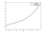
(a) Comparison between $w(0.5,t)$ and $\hat{w}(0.5,t)$

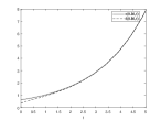
(b) Comparison between $v(0.5,t)$ and $\hat{v}(0.5,t)$

Figure 5: A comparison between the states of the coupled system (1)-(4) versus the estimated states using observer (42) at $x=0.56$. System parameters are $\gamma=1$, $\rho=0.5$, $\alpha=1$, $\beta=1$ , $o_{2}=5$ with initial conditions $w_{0}=\sin(\pi x)$ and $\hat{w}_{0}=\cos(\pi x)$.

$L_{2}$-norm of the error dynamics (45) using two measurements $w(1,t),\;v(1,t)$

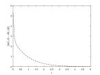
(a) $\|w(\cdot,t)-\hat{w}(\cdot,t)\|$

(b) $\|v(\cdot,t)-\hat{v}(\cdot,t)\|$

Figure 6: $L_{2}$-norms of the error dynamics of the estimates of the parabolic and elliptic states, using two measurements $w(1,t),\;v(1,t).$ System parameters are $\gamma=1$, $\rho=0.5$, $\alpha=1$, $\beta=1$ , $o_{2}=5$ with initial conditions $w_{0}=\sin(\pi x)$ and $\hat{w}_{0}=\cos(\pi x)$. The estimation error tends to $0$ as $t\to\infty.$

Numerical simulations were also conducted to study the observer (64) when a single measurement $w(1,t)$ available. The simulations were carried out using the parameter values $\gamma=1$, $\rho=1$, $\alpha=0.5$, $\beta=0.5$. With these parameter values, the system is stable. Also, we set $o_{2}=0.5$ so the stability condition for the observation error dynamics (i.e. (86)) is satisfied. The control input $u(t)$ was set as stated in (40), with control gain $c_{2}=0.5$. The initial conditions were $w_{0}=\sin(\pi x)$ and $\hat{w}_{0}=\sin(2\pi x).$ The true and estimated states at $x=0.56$ are given in Figure7. The $L_{2}$-norms of the error dynamics are presented in Figure8.

True and estimated states at $x=0.56$ using observer (64)

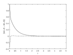
(a) Comparison between $w(0.5,t)$ and $\hat{w}(0.5,t)$

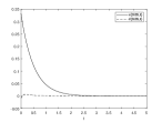
(b) Comparison between $v(0.5,t)$ and $\hat{v}(0.5,t)$

Figure 7: A comparison between the states of the coupled system (1)-(4) versus the estimated states using observer (64) at $x=0.56$. Here $\gamma=1$, $\rho=1$, $\alpha=0.5$, $\beta=0.5$ , $o_{2}=c_{2}=0.5$ with $w_{0}=\sin(\pi x)$ and $\hat{w}_{0}=\sin(2\pi x)$.

$L_{2}$-norm of the error dynamics (65), using one measurements $w(1,t)$

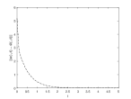
(a) $\|w(x,t)-\hat{w}(x,t)\|$

(b) $\|v(x,t)-\hat{v}(x,t)\|$

Figure 8: $L_{2}$-norms of the error dynamics of the estimates of the parabolic and elliptic states, using a single measurement $w(1,t).$ Here $\gamma=1$, $\rho=1$, $\alpha=0.5$, $\beta=0.5$ and $o_{2}=c_{2}=0.5$ with $w_{0}=\sin(\pi x)$ and $\hat{w}_{0}=\sin(2\pi x)$. The estimation error tends to $0$ as $t\to\infty.$

5 Output feedback

In general, the full state is not available for control. Output feedback is based on using only the available measurements to stabilize the system. A common approach to output feedback is to combine a stabilizing state feedback with an observer. The estimated state from the observer is used to replace the state feedback $Kz$ by $K\hat{z}$ where $z$ is the true state and $\hat{z}$ the estimated state.

In the situation considered here, if there are two measurements, this leads to the output feedback controller consisting of the observer (42) combined with the state feedback

$$u(t)=\int_{0}^{1}k^{a}_{x}(1,y)\hat{w}(y,t)dy+k^{a}(1,1)\hat{w}(1,t)$$ (87)

where $k^{a}(x,y)$ is the solution of system (15) with $c_{2}$ satisfying the bound (41). Since the original system (1)-(4) is a well-posed control system (Theorem 1)and also the observer combined with the state feedback is a well-posed system, the following result follows immediately from the results in [20, section 3].

Theorem 19.

The closed-loop system consisting of (1)-(4), together with the observer dynamics (42) and control input (87), is well-posed and exponentially stable.

Note that when using output feedback, the parameters have to satisfy both of the stability condition associated with the control problem (41), and also the bound of the stability of the observation error (63).

5.1 Numerical simulations

Numerical simulations, again using a finite-element approximation in the COMSOL Multiphysics software, were performed to study the solutions of system (1)-(4) with output feedback (87). The parameter values were $\gamma=\frac{1}{4}$, $\rho=\frac{1}{3}$, $\alpha=\frac{1}{4}$, and $\beta=\frac{1}{2}$. The system’s initial condition was $w_{0}=\sin(\pi x)$.With these parameters, the uncontrolled system is unstable.

To achieve stability, the control gain $c_{2}=1.2-\rho$, ensuring that the stability condition (41) is satisfied. Additionally, to ensure exponential stability of the error dynamics $o_{2}=3$, which satisfies inequality (63). However, after applying control, the state of the coupled system converges to the steady-state solution; see Figure9. This convergence is clearly depicted in the comparison shown in Figure10, where we compare the $L_{2}$- norm of the controlled and uncontrolled states.

Dynamics of closed-loop system with output feedback

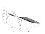
(a) $w(x,t)$

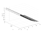
(b) $v(x,t)$

Figure 9: A 3D landscape of the dynamics of a controlled coupled parabolic-elliptic system (1)-(4) after applying the output feedback control input (87). The uncontrolled system is unstable, but the use of output feedback leads to an exponentially stable closed-loop system.

Comparison of open-loop and closed-loop $L_{2}$-norms with output feedback

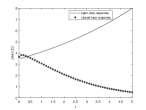
(a) $L_{2}$-norm $\|w(\cdot,t)\|$

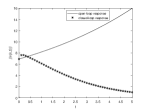
(b) $L_{2}$-norm $\|v(\cdot,t)\|$

Figure 10: A comparison between the $L_{2}$-norms of $w(x,t)$ and $v(x,t)$ for the uncontrolled system and the system controlled with output feedback. Without control, the norms of both states grow, due to instability. However, with output feedback control, both states decay to zero.

6 Conclusion

Stabilization of systems composed of coupled parabolic and elliptic equations presents considerable challenges. The first part of this paper considers the boundary stabilization of a linear coupled parabolic-elliptic system. Previous literature has shown that coupling between the equations can result in an unstable system. Previous work on stabilization via two boundary control inputs was used in [16]. In this paper we used a single control input to stabilize both equations. Deriving one control law that stabilizes the system posed several challenges. One approach is to rewrite the coupled system into one equation in terms of the parabolic state. But due to the appearance of a Fredholm operator, this makes it difficult to establish a suitable kernel for the backstepping transformation. Using separate transformations for each of the parabolic and the elliptic states would be quite complicated. In this paper we transformed only the parabolic part of the system, which simplified the calculations. This enabled reuse of a previously calculated transformation. However, the price is that this transformation mapped the original coupled system into a complicated target system which further complicated showing stability of the target system. Lyapunov theory was used to obtain a sufficient condition for stability of the target system.

The second part of the paper focused on the observer design problem. Several synthesises are proposed depending on the available measurements. Output injections were chosen so that the exponential stability of the observation error dynamics is ensured. Again, instead of looking for a new state transformation that maps the original error dynamics into an exponentially stable target system, well-known transformations in the literature are employed. Then, the exponential stability of the original error dynamics is shown by establishing suitable sufficient conditions for stability. The key to obtaining a stability condition was again to use Lyapunov theory. As for controller design, the technical conditions for observer design depend on the number of the available measurements. When measurements for both states were provided, two transformations were applied to both parabolic and elliptic states of the error dynamics. A total of four filters, two throughout the domain and two at the boundary, were needed. On the other hand, when a single measurement for the parabolic state is given, one boundary filter was designed for the parabolic equation. However, in the latter case, a more restrictive condition for stability of the error dynamics was obtained. Observer design with a single sensor parallels to a great extent that of stabilization via one control signal. Showing exponential stability of the target error dynamics, in the situation when one measurement is provided, results in a very restrictive constraint on the parameters of the coupled system.

In a final section, control and observation were combined to obtain an output feedback controller. The results were again illustrated with simulations.

In this paper, the control as well as the observer gains were designed at $x=1$. The situation is similar when the control and the observer gains are placed at $x=0$, although different backstepping transformations are needed. This is covered in detail in [4].

Open questions include finding weaker sufficient conditions for stability of both the controller and the observer. Future work is aimed at improving the conditions on the control parameter $c_{2}$ concerning the boundary stabilization problem. Similarly, relaxing stability condition on the parameters for the observer design problem with a single measurement is of interest. In many problems, the equations are nonlinear and design of a boundary control for a nonlinear coupled parabolic-elliptic equations will also be studied.

References

• [1] Ole Morten Aamo. Disturbance rejection in 2 x 2 linear hyperbolic systems. IEEE transactions on automatic control, 58(5):1095–1106, 2012.
• [2] Jaewook Ahn and Changwook Yoon. Global well-posedness and stability of constant equilibria in parabolic–elliptic chemotaxis systems without gradient sensing. Nonlinearity, 32(4):1327, 2019.
• [3] Alalabi Ala’ and Morris Kirsten. Stabilization of a parabolic-elliptic system via backstepping. In the proceedings of the 2023 Conference on Decision and Control, 2023.
• [4] Ala’ Alalabi. Stability, Stabilization and Observer Design for a Class of Partial Differential-Algebraic Equations. PhD thesis, University of Waterloo, Canada, in prepartion.
• [5] Antonello Baccoli and Alessandro Pisano. Anticollocated backstepping observer design for a class of coupled reaction-diffusion pdes. Journal of Control Science and Engineering, 2015:53–53, 2015.
• [6] Antonello Baccoli, Alessandro Pisano, and Yury Orlov. Boundary control of coupled reaction–diffusion processes with constant parameters. Automatica, 54:80–90, 2015.
• [7] Philippe Benilan, Petra Wittbold, et al. On mild and weak solutions of elliptic-parabolic problems. Advances in Differential Equations, 1(6):1053–1073, 1996.
• [8] Giuseppe Maria Coclite, Helge Holden, and Kenneth H Karlsen. Wellposedness for a parabolic-elliptic system. Discrete & Continuous Dynamical Systems-A, 13(3):659, 2005.
• [9] Luisa Consiglieri. Weak solutions for multiquasilinear elliptic–parabolic systems: application to thermoelectrochemical problems. Boletín de la Sociedad Matemática Mexicana, 26(2):535–562, 2020.
• [10] Ruth Curtain and Hans Zwart. Introduction to infinite-dimensional systems theory: a state-space approach, volume 71. Springer Nature, 2020.
• [11] Agus Hasan, Ole Morten Aamo, and Miroslav Krstic. Boundary observer design for hyperbolic pde–ode cascade systems. Automatica, 68:75–86, 2016.
• [12] Birgit Jacob and Kirsten Morris. On solvability of dissipative partial differential-algebraic equations. IEEE Control Systems Letters, 6:3188–3193, 2022.
• [13] Yushan Jiang, Chao Liu, Qingling Zhang, and Tieyu Zhao. Two side observer design for singular distributed parameter systems. Systems & Control Letters, 124:112–120, 2019.
• [14] Shumon Koga, Mamadou Diagne, Shuxia Tang, and Miroslav Krstic. Backstepping control of the one-phase stefan problem. In 2016 American Control Conference (ACC), pages 2548–2553, 2016.
• [15] Miroslav Krstic, Antranik A Siranosian, and Andrey Smyshlyaev. Backstepping boundary controllers and observers for the slender timoshenko beam: Part i-design. In 2006 American Control Conference, pages 2412–2417. IEEE, 2006.
• [16] Miroslav Krstic and Andrey Smyshlyaev. Boundary control of PDEs: A course on backstepping designs. SIAM, 2008.
• [17] Bin Li. Global existence and decay estimates of solutions of a parabolic–elliptic–parabolic system for ion transport networks. Results in Mathematics, 75(2):45, 2020.
• [18] Tetyana Malysheva and Luther W White. Global well-posedness theory for a class of coupled parabolic-elliptic systems. Journal of Mathematical Analysis and Applications, 486(2):123923, 2020.
• [19] Hannes Meinlschmidt, Christian Meyer, and Joachim Rehberg. Optimal control of the thermistor problem in three spatial dimensions, part 1: existence of optimal solutions. SIAM Journal on Control and Optimization, 55(5):2876–2904, 2017.
• [20] Kirsten A Morris. State feedback and estimation of well-posed systems. Mathematics of Control, Signals and Systems, 7(4):351–388, 1994.
• [21] Scott Moura, Jan Bendtsen, and Victor Ruiz. Observer design for boundary coupled pdes: Application to thermostatically controlled loads in smart grids. In 52nd IEEE conference on decision and control, pages 6286–6291. IEEE, 2013.
• [22] Mihaela Negreanu, Jose Ignacio Tello, and Antonio Manuel Vargas. On a parabolic-elliptic chemotaxis system with periodic asymptotic behavior. Mathematical Methods in the Applied Sciences, 42(4):1210–1226, 2019.
• [23] H. Parada, E. Cerpa, and K. A. Morris. Feedback control of an unstable parabolic-elliptic system with input delay. preprint, 2020.
• [24] Andrey A Polezhaev, Ruslan A Pashkov, Alexey I Lobanov, and Igor B Petrov. Spatial patterns formed by chemotactic bacteria escherichia coli. International Journal of Developmental Biology, 50(2-3):309–314, 2003.
• [25] Andrey Smyshlyaev and Miroslav Krstic. Backstepping observers for a class of parabolic pdes. Systems & Control Letters, 54(7):613–625, 2005.
• [26] Georgy A Sviridyuk and Vladimir E Fedorov. Linear Sobolev type equations and degenerate semigroups of operators. de Gruyter, 2003.
• [27] Youshan Tao and Michael Winkler. Boundedness vs. blow-up in a two-species chemotaxis system with two chemicals. Discrete Contin. Dyn. Syst. Ser. B, 20(9):3165–3183, 2015.
• [28] Bernd Thaller and Sigrid Thaller. Factorization of degenerate cauchy problems: The linear case. Journal of Operator Theory, pages 121–146, 1996.
• [29] Roberto Triggiani. On the stabilizability problem in banach space. Journal of Mathematical Analysis and Applications, 52(3):383–403, 1975.
• [30] Sascha Trostorff. Semigroups associated with differential-algebraic equations. In Semigroups of Operators–Theory and Applications: SOTA, Kazimierz Dolny, Poland, September/October 2018, pages 79–94. Springer, 2020.
• [31] Rafael Vázquez and Miroslav Krstić. Boundary control of coupled reaction-advection-diffusion systems with spatially-varying coefficients. IEEE Transactions on Automatic Control, 62:2026–2033, 2016.
• [32] Rafael Vazquez, Miroslav Krstic, and Jean-Michel Coron. Backstepping boundary stabilization and state estimation of a 2$\times$ 2 linear hyperbolic system. In 2011 50th IEEE conference on decision and control and european control conference, pages 4937–4942. IEEE, 2011.
• [33] Yilong Wang. A quasilinear attraction–repulsion chemotaxis system of parabolic–elliptic type with logistic source. Journal of Mathematical Analysis and Applications, 441(1):259–292, 2016.
• [34] Jinbiao Wu, Jinchao Xu, and Henghui Zou. On the well-posedness of a mathematical model for lithium-ion battery systems. Methods and Applications of Analysis, 13(3):275–298, 2006.