Few-shot Diagnosis of Chest x-rays Using an Ensemble of Random Discriminative Subspaces

Abstract

Due to the scarcity of annotated data in the medical domain, few-shot learning may be useful for medical image analysis tasks. We design a few-shot learning method using an ensemble of random subspaces for the diagnosis of chest x-rays (CXRs). Our design is computationally efficient and almost 1.8 times faster than method that uses the popular truncated singular value decomposition (t-SVD) for subspace decomposition. The proposed method is trained by minimizing a novel loss function that helps create well-separated clusters of training data in discriminative subspaces. As a result, minimizing the loss maximizes the distance between the subspaces, making them discriminative and assisting in better classification. Experiments on large-scale publicly available CXR datasets yield promising results. Code for the project will be available at https://github.com/Few-shot-Learning-on-chest-x-ray/fsl˙subspace.

1 Introduction

Few-shot Learning Snell et al. (2017); Chen et al. (2019); Wang et al. (2020) aims to learn new tasks with small annotated samples per class. Most modern deep learning methods require a large number of annotated training samples. However, large annotated medical image datasets are often elusive because of various factors including cost and human efforts involved. Therefore, few-shot learning may be useful for medical image analysis. Few-shot learning techniques are often designed using either meta-learning Finn et al. (2017); Zhang et al. (2018); Ren et al. (2018) or metric learning Vinyals et al. (2016); Simon et al. (2020) based approaches.

In this paper, we present a method for a few-shot diagnosis of chest x-ray (CXR) images using an ensemble of random subspaces. Our method consists of three stages, namely, a feature extraction module (FEM) that extracts visual feature vectors from x-ray images, a subspace embedding module (SEM) to project the feature vectors into multiple random discriminative subspaces, and a final decision module (FDM) that assigns a final class label to an input x-ray image based on the projections. The SEM in the proposed method aims to create an ensemble of discriminative subspaces to explore different combinations of visual features obtained from small data samples. To that end, our method generates subspaces having low similarity with each other. Such subspaces with low correlation are likely to aid ensemble learning Breiman (2001).

In this paper, we make the following major contributions: $i$) We propose a method for the few-shot chest x-ray diagnosis using an ensemble of random subspaces. $ii)$ Our method consists of multiple modules along with a novel loss component that makes these subspaces class discriminative, resulting in improved classification accuracy. $iii)$ The proposed method provides a faster alternative to existing computationally intensive subspace decomposition techniques such as truncated singular value decomposition (t-SVD) Li et al. (2019).

The rest of the paper is organized as follows: Section 2 provides the details of the proposed method. The experiments and results are described in Section 3. In Section 4, we conclude the paper. Finally, we describe the implementation details along with the ablation studies in the appendices.

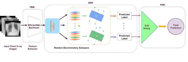
Figure 1: Pipeline of the proposed method. Our model consists of a feature extraction module (FEM), a subspace embedding module (SEM), and a final decision module (FDM). FEM extracts visual features from the chest x-ray images. SEM projects the extracted feature vectors into multiple random subspaces, each of which assigns a class label to the input x-ray. These labels are then used by FDM to produce the final output label.

2 Methods

In the standard few-shot classification setting, we define a support set $S=(x_{1},y_{1}),...,(x_{K},y_{K})$ and a query set $Q=(x^{\prime}_{1},y^{\prime}_{1}),...,(x^{\prime}_{K^{\prime}},y^{\prime}_{K^{\prime}})$ of $K$ and $K^{\prime}$ labelled points respectively. Here each $x_{i}$ and $x^{\prime}_{i}$ are $D-$dimensional feature vectors and $y_{i}$ and $y^{\prime}_{i}$ are the corresponding class labels, respectively. The problem is formulated as $N$-way $K$-shot, where $N$ represents the number of classes in the support set, while $K$ denotes the number of examples of each class. The optimizations iterate in an episodic fashion taking one update at a time. In addition, the model parameters are updated by minimizing the loss function. Our model consists of three modules, namely the Feature extraction module (FEM), the Subspace embedding module (SEM), and the Final decision module (FDM). A block diagram of the proposed method is presented in Fig. 1.

2.1 Feature extraction module (FEM)

FEM is used for extracting visual features from chest x-rays. To design the FEM, we use a feature extractor, pre-trained on the ImageNet Russakovsky et al. (2015) dataset. The FEM, designed using the EfficientNet-B7 backbone Tan & Le (2019) is further fine-tuned using x-ray images in concert with the other modules. The extracted feature vectors are then fed into the SEM.

2.2 Subspace Embedding Module (SEM)

The subspace embedding module maps an input feature vector (obtained from FEM) to an ensemble of subspaces. Consider an embedding function $E_{\theta,\nu}$ an ${D}$-dimensional input feature vector to a ${N}$-dimensional feature vector in subspace $\nu$. This embedding function is implemented through fully connected layers with parameters $\theta$. Consider class $j$. We calculate the mean embedding for class $j$ at subspace $\nu$ considering all the support points belonging to class $j$. The mean embedding is

$$\lambda_{j}(\nu)=\frac{1}{C_{j}}\sum_{a_{i}\in j}E_{\theta,\nu}\left(a_{i}\right),$$ (1)

where $a_{i}$ is the $i^{\textrm{th}}$ data point belonging to class $j$ and $C_{j}$ is the number of support points in class $j$. The Euclidean distance between the mean embedding and the query point $q$ is

$$R_{j}(q,\nu)=\left\|E_{\theta,\nu}\left(q\right)-\lambda_{{j}}(\nu)\right\|_{2},$$ (2)

where, $\left\|.\right\|_{2}$ represent the L2-norm. Further, by applying the softmax on (2) in subspace $\nu$, we obtain the probability that query point $q$ belongs to class $j$

$$S_{j}(\nu)=\frac{e^{-R_{j}(\nu)}}{\sum_{j}e^{-R_{j}(\nu)}}.$$ (3)

Thus, for the query point, we may find the class probabilities for all classes at each subspace. We aim to utilize complimentary information from the extracted feature vectors through an ensemble of subspaces. To that end, we want every pair of subspaces to be discriminative and have less similarities with each other. The similarities are captured through a discriminative loss which is minimized in our method. Consider subspaces $x$ and $y$. Let the parameters of the neural network layers mapping to these subspaces be $\theta_{x}$ and $\theta_{y}$, respectively. Then the discriminative loss is

$$\mathcal{L}_{dis}=\sum_{\forall x,y}\frac{\theta_{x}\cdot\theta_{y}}{\left|\theta_{x}\right|\left|\theta_{y}\right|},$$ (4)

where $\cdot$ indicates a scalar product. Minimization of the above loss function helps in making the subspaces discriminative. The class probabilities from (3) are next used by the final decision module.

2.3 Final decision module (FDM)

The FDM uses the class probabilities from the subspaces. The class label with the highest vote from the subspaces is considered to be the final output label for an input CXR image. Using the output labels from FDM and the ground truth labels, we compute a cross-entropy loss $\mathcal{L}_{sup}$ for the support set images of the training classes. Also, using the output labels from FDM for the query images of the training classes, we compute a cross-entropy loss $\mathcal{L}_{qur}$. Hence, the total loss is

$$\mathcal{L}=\mathcal{L}_{{sup}}+\alpha\mathcal{L}_{{qur}}+\beta\mathcal{L}_{{dis}},$$ (5)

where $\alpha$ and $\beta$ are predefined constants. Our model is trained by minimizing the above loss.

2.4 Testing

We randomly select five image samples from each test class for testing and compute the cluster center based on those five images for each test class. Query image are then taken from the test classes, and our model projects each query images onto randomly selected subspaces. Every subspace assigns a class label to a query image as discussed in Section 2.2. The final class label for a query image is obtained by soft voting using the class probabilities.

Figure 2: Sample results of the prediction (P) by the proposed method and the ground truth (GT) for images of novel classes. Correct and incorrect detections are marked in green and red, respectively.

3 Results

3.1 Datasets and Experimental Settings

We perform experiments on the publicly available NIH chest x-ray dataset Wang et al. (2017) which contains frontal CXR images with 14 different types of thoracic abnormalities. We only take images with single abnormalities for our experiments. Atelectasis, consolidation, infiltration, pneumothorax, fibrosis, effusion, pneumonia, pleural thickening, nodule, mass, hernia, edema, emphysema, and cardiomegaly are among the 14 thorax disorders or conditions studied. When a sample does not contain any abnormality, it is labeled as ‘NoFinding’. We have considered five groups with different combinations of training, validation, and test classes. At each group, three test classes, three validation classes, and nine training classes are selected randomly without replacement, ensuring that these classes do not overlap. We also ensure that the test classes across different groups do not overlap so that every class is used for testing in some experiment. A detailed description of the groups is presented in appendix A (see Table 3). Furthermore, we evaluate our model’s performance on multiple random subspaces by conducting experiments with varying numbers of subspaces under the same conditions. Our findings indicate that using 30 ($\nu$ = 30) subspaces leads to improved performance.

Table 1: Accuracy of 3-way 5-shot classification with 95% confidence interval on the different combinations of test/novel classes of the NIH dataset for different methods. The different combinations are represented by different groups mentioned in appendix A

Group	Abnormality	ProtoNet	MatchingNet	MAML	DSN	Proposed
	Fibrosis	44.24±1.52	38.04±1.89	42.80±0.43	38.94±1.48	42.82±1.75
Group1	Hernia	44.34±1.50	38.24±1.89	16.85±0.30	43.38±1.51	30.10±1.62
	Pneumonia	45.68±1.55	30.43±1.89	44.89±0.44	50.28±1.57	40.88±1.66
	Mass	34.78±1.47	34.00±1.85	41.94±0.44	38.34±1.50	35.68±1.42
Group2	Nodule	34.86±1.46	34.60±1.87	14.65±0.28	35.84±1.48	35.96±1.48
	Pleural Thickening	34.48±1.45	34.56±1.87	43.85±0.45	33.08±1.44	31.08±1.41
	Cardiomegaly	52.58±1.78	45.04±2.38	38.42±0.43	45.94±1.54	38.62±1.54
Group3	Edema	54.18±1.79	47.96±2.37	39.21±0.41	68.00±1.47	65.16±1.48
	Emphysema	54.64±1.77	47.04±2.41	34.60±0.43	49.08±1.60	42.04±1.61
	Consolidation	39.62±1.50	41.80±1.86	25.17±0.37	38.98±1.54	32.84±1.58
Group4	Effusion	41.26±1.60	40.06±1.84	22.30±0.35	42.82±1.54	38.20±1.61
	Pneumothorax	24.94±1.55	40.42±1.82	56.01±0.43	44.98±1.59	49.98±1.74
	Atelectasis	38.14±1.50	36.46±1.66	44.21±0.45	37.72±1.53	27.98±1.44
Group5	Infiltration	38.36±1.50	36.28±1.65	11.39±0.23	37.22±1.55	35.94±1.50
	No Finding	24.92±1.54	38.06±1.72	45.98±0.46	38.86±1.52	52.84±1.71

Table 2: Comparison of the training time (1 epoch) of the proposed method with the DSN Simon et al. (2020) involving truncated SVD. The experiments have been executed using Nvidia-GeForce GTX 1080Ti GPU with 11,178 MiB memory.

Method	Approach	Train time	Hardware specs
Proposed	Ensemble of Random Subspace	18 min 35 sec	GTX 1080 Ti
DSN	Truncated Singular Value Decomposition (t-SVD)	33 min 48 sec	GTX 1080 Ti

3.2 Comparative Performances

We compare the performance of our method with several state-of-the-art few-shot learning methods, including Prototypical Network (ProtoNet) Snell et al. (2017), Matching Network (MatchingNet) Vinyals et al. (2016), MAML Finn et al. (2017), and Adaptive Subspace (DSN) Simon et al. (2020). The results are evaluated using 15 query images for 3-way 5-shot classification in terms of mean average accuracy with a 95% confidence interval and reported in Table 1 for the test/novel classes listed in the appendix A (see Table 3). Notice that our approach yields better or comparable performance in terms of accuracy for a number of the novel classes. This shows the effectiveness of our method for the few-shot diagnosis of CXRs.

The proposed method is also faster than DSN which uses the t-SVD as the subspace decomposition technique. The running time of our method is compared in Table 2 with that of DSN Simon et al. (2020). It can be observed that the proposed method is approximately $\sim 1.8$ faster in a single epoch. This speed-up is due to the use of random subspaces in our method. A complexity analysis of the proposed method (see appendix D) with t-SVD demonstrates the advantage in terms of computational efficiency over t-SVD based methods.

4 Conclusions

We propose a few-shot learning model using random discriminative subspaces for chest x-ray diagnosis. The use of random subspaces makes our method a faster alternative to compute-intensive methods like t-SVD. Experiments and ablation studies demonstrate the utility of our method, which employs novel loss functions to aid in the generation of discriminative subspaces. In the future, we will explore the possibility of using auxiliary information about different abnormalities to aid the classification. We would also look into developing generalizable few-shot learning models for chest x-ray diagnosis.

Appendix A Combination of abnormalities for different experiment

The description below details the combination of anomalies for different experiments, which are conducted separately for each group.

Table 3: Combinations of the train/base, validation, and test/novel classes from Group1 to Group5 of the NIH dataset.

Group	Train/Base Class	Validation Class	Test/Novel Class
Group1	Mass, Edema, Cardiomegaly, Effusion, Infiltration, Nodule, Emphysema, No Finding, Pneumothorax	Atelectasis, Consolidation, Pleural Thickening	Hernia, Pneumonia, Fibrosis
Group2	Effusion, Consolidation, Edema, Cardiomegaly, No Finding, Atelectasis, Infiltration, Emphysema, Pneumothorax	Fibrosis, Hernia, Pneumonia	Mass, Nodule, Pleural Thickening
Group3	Pneumothorax, Consolidation, Hernia, No Finding, Atelectasis, Infiltration, Effusion, Pneumonia, Fibrosis	Mass, Nodule, Pleural Thickening	Emphysema, Edema, Cardiomegaly
Group4	Infiltration, Hernia, Fibrosis, No Finding, Atelectasis, Nodule, Mass, Pneumonia, Pleural Thickening	Emphysema, Edema, Cardiomegaly	Consolidation, Effusion, Pneumothorax
Group5	Hernia, Fibrosis, Pneumonia, Pleural Thickening, Nodule, Mass, Emphysema, Edema, Cardiomegaly	Consolidation, Effusion, Pneumothorax	Infiltration, Atelectasis, No Finding

Appendix B Implementation Details

The feature extraction module is designed using EfficientNet-B7 Tan & Le (2019). The network module for projecting the input feature vector into subspaces comprises of linear and batch normalization layers. The 1000-dimensional feature space obtained from the input image using the feature extractor is then mapped to 512-dimension and further to 64-dimensional embedding. Using the chest x-rays as our training data, we perform end-to-end training on the ImageNet pre-trained model for 80 epochs consisting of 1000 batches with a single episode per batch with cross-entropy loss as the loss function. Further, we assume that the constants $\alpha$ and $\beta$ are equal to 1 for the loss calculation described in (5).

Appendix C Ablation Studies

We perform several ablation studies to evaluate the effectiveness of different aspects of the model that contribute to yielding better performance over existing techniques.

C.1 On the Components of the Loss Functions

We look into the effect of different components of the loss functions described in (5). To that end, we experiment only with the cross-entropy loss using the query points ($\mathcal{L}_{{qur}}$). Subsequently, we also introduce another component of cross-entropy loss using the support set ($\mathcal{L}_{{sup}}$). The added loss term is likely to enforce the samples from the support classes to move closer around the mean embeddings, thereby helping to obtain better cluster representation which further helps in generalization. Next, we also introduce a cosine similarity-based loss term to maximize the separation between the weights matrix of the subspace, making them more discriminative. As a result, minimizing the loss function maximizes the distances between the subspaces, which further aids in better classification. The results of these studies are presented in Table 4. Notice that our method outperforms the model either using $\mathcal{L}_{{qur}}$ or $\mathcal{L}_{{qur}}+\mathcal{L}_{{sup}}$ loss for nine novel classes. Hence, we conclude that each loss term in the proposed method contributes to improved performance.

Table 4: Results of ablation studies in terms of classification accuracy with 95% confidence interval for different combinations of the loss components. We compare our method (Proposed Loss) that comprises of ($\mathcal{L}_{\text{qur }}+\mathcal{L}_{\text{sup }}+\mathcal{L}_{\text{dis }}$) with Loss1 ($\mathcal{L}_{\text{qur }}$) and Loss2 ($\mathcal{L}_{\text{qur }}+\mathcal{L}_{\text{sup }}$) respectively.

Group	Abnormality	Loss1	Loss2	Proposed Loss
	Fibrosis	45.18±1.61	46.74±1.91	42.82±1.75
Group1	Hernia	35.62±1.42	30.04±1.65	30.10±1.62
	Pneumonia	39.88±1.55	38.38±1.58	40.88±1.66
	Mass	34.08±1.49	32.42±1.45	35.68±1.42
Group2	Nodule	38.42±1.54	36.90±1.52	35.62±1.48
	Pleural Thickening	29.88±1.38	30.94±1.41	31.08±1.41
	Cardiomegaly	38.18±1.51	37.78±1.54	38.20±1.54
Group3	Edema	65.94±1.48	57.66±1.54	65.16±1.48
	Emphysema	40.02±1.58	40.66±1.58	42.04±1.61
	Consolidation	31.84±1.56	35.58±1.50	32.84±1.58
Group4	Effusion	39.10±1.69	41.82±1.59	38.20±1.61
	Pneumothorax	45.62±1.91	42.72±1.62	49.98±1.74
	Atelectasis	29.60±1.38	30.92±1.45	27.98±1.44
Group5	Infiltration	35.08±1.49	35.74±1.49	35.94±1.50
	No Finding	50.70±1.62	46.34±1.73	52.84±1.71

C.2 Role of the Random Subspace

Besides selecting the appropriate number of random subspaces, we also intend to evaluate the significance of random subspaces in obtaining better performance than other methods. Accordingly, we ran the experiment with the model without subspaces and compared it with our method in terms of F1-score. From the experiment results in Fig. 3, it is evident that the proposed method outperforms the model with no subspace for eight novel classes while obtaining comparable results for the rest of the classes, thereby helping obtain better results. This can be explained by the fact that the feature space contains both important and redundant features. The presence of unimportant features reduces the classifier’s performance. Thus, by employing an ensemble of the subspace, we intend to investigate various combinations of features that result in improved classification accuracy.

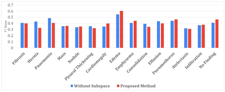
Figure 3: Comparative performance of the proposed method using random subspace (Proposed) and single feature subspace instead of random subspace (Without subspace) in terms of F1 score.

C.3 Choice of The Feature Extractor

We investigate the impact of feature extractor choice by comparing our EfficientNet-B7 feature extractor to DenseNet-121 Huang et al. (2017). Table 5 reveals that using EfficientNet-B7 outperforms DenseNet-121 in terms of mean average accuracy for eight novel classes, while having similar performance for the others. This improvement is due to the uniform scaling of network parameters, such as depth, width, and resolution, using a compound coefficient Tan & Le (2019). Hence, our findings suggest that EfficientNet-B7 as the feature extractor leads to better generalization for novel classes than the DenseNet-121 backbone.

Table 5: Accuracy of 3-way 5-shot classification with 95% confidence interval for our proposed method (Proposed) with EfficientNet-B7 backbone alongside with DenseNet-121 feature extractor for subspace 30.

Group	Abnormality	DenseNet-121	Proposed
	Fibrosis	39.78±1.69	42.82±1.75
Group1	Hernia	38.00±1.71	30.10±1.62
	Pneumonia	43.00±1.60	40.88±1.66
	Mass	33.48±1.42	35.68±1.42
Group2	Nodule	34.90±1.41	35.62±1.48
	Pleural Thickening	36.24±1.46	31.08±1.41
	Cardiomegaly	37.68±1.52	38.20±1.54
Group3	Edema	59.56±1.60	65.16±1.48
	Emphysema	36.80±1.49	42.04±1.61
	Consolidation	38.56±1.52	32.84±1.58
Group4	Effusion	42.62±1.58	38.20±1.61
	Pneumothorax	37.22±1.45	49.98±1.74
	Atelectasis	29.74±1.43	27.98±1.44
Group5	Infiltration	38.54±1.58	35.94±1.50
	No Finding	43.82±1.63	52.84±1.71

Appendix D On the Computational Complexity

We evaluate the time complexity of the proposed method which utilizes an ensemble of random subspaces for subspace decomposition in comparison to t-SVD. The time complexity of the t-SVD technique is $\mathcal{O}\left(2ab^{2}+b^{3}+b+ab\right)$ Li et al. (2019), where $a$ is the number of data points and $b$ is the dimension of the feature vectors. With the assumption that the dimension of the feature vectors are constant, the time complexity can be simplified to $\mathcal{O}(a)$. On the other hand, for our method, the subspaces are generated randomly. As a result, the subspace generation process in the proposed method is independent of the number of data points. Therefore, w.r.t. the number of data points, the time complexity of the proposed method is $\mathcal{O}(1)$. Thus, we find that in terms of time complexity, the subspace decomposition in the proposed method has a better performance compared to the t-SVD.

References

- Breiman (2001) Leo Breiman. Random forests. Machine learning, 45(1):5–32, 2001.
- Chen et al. (2019) Wei-Yu Chen, Yen-Cheng Liu, Zsolt Kira, Yu-Chiang Frank Wang, and Jia-Bin Huang. A closer look at few-shot classification. arXiv preprint arXiv:1904.04232, 2019.
- Finn et al. (2017) Chelsea Finn, Pieter Abbeel, and Sergey Levine. Model-agnostic meta-learning for fast adaptation of deep networks. In International conference on machine learning, pp. 1126–1135. PMLR, 2017.
- Huang et al. (2017) Gao Huang, Zhuang Liu, Laurens Van Der Maaten, and Kilian Q Weinberger. Densely connected convolutional networks. In Proceedings of the IEEE conference on computer vision and pattern recognition, pp. 4700–4708, 2017.
- Li et al. (2019) Xiaocan Li, Shuo Wang, and Yinghao Cai. Tutorial: Complexity analysis of singular value decomposition and its variants. arXiv preprint arXiv:1906.12085, 2019.
- Ren et al. (2018) Mengye Ren, Eleni Triantafillou, Sachin Ravi, Jake Snell, Kevin Swersky, Joshua B Tenenbaum, Hugo Larochelle, and Richard S Zemel. Meta-learning for semi-supervised few-shot classification. arXiv preprint arXiv:1803.00676, 2018.
- Russakovsky et al. (2015) Olga Russakovsky, Jia Deng, Hao Su, Jonathan Krause, Sanjeev Satheesh, Sean Ma, Zhiheng Huang, Andrej Karpathy, Aditya Khosla, Michael Bernstein, et al. Imagenet large scale visual recognition challenge. International journal of computer vision, 115(3):211–252, 2015.
- Simon et al. (2020) Christian Simon, Piotr Koniusz, Richard Nock, and Mehrtash Harandi. Adaptive subspaces for few-shot learning. In Proceedings of the IEEE/CVF Conference on Computer Vision and Pattern Recognition, pp. 4136–4145, 2020.
- Snell et al. (2017) Jake Snell, Kevin Swersky, and Richard Zemel. Prototypical networks for few-shot learning. Advances in neural information processing systems, 30, 2017.
- Tan & Le (2019) Mingxing Tan and Quoc Le. Efficientnet: Rethinking model scaling for convolutional neural networks. In International conference on machine learning, pp. 6105–6114. PMLR, 2019.
- Vinyals et al. (2016) Oriol Vinyals, Charles Blundell, Timothy Lillicrap, Daan Wierstra, et al. Matching networks for one shot learning. Advances in neural information processing systems, 29, 2016.
- Wang et al. (2017) Xiaosong Wang, Yifan Peng, Le Lu, Zhiyong Lu, Mohammadhadi Bagheri, and Ronald M Summers. Chestx-ray8: Hospital-scale chest x-ray database and benchmarks on weakly-supervised classification and localization of common thorax diseases. In Proceedings of the IEEE conference on computer vision and pattern recognition, pp. 2097–2106, 2017.
- Wang et al. (2020) Yaqing Wang, Quanming Yao, James T Kwok, and Lionel M Ni. Generalizing from a few examples: A survey on few-shot learning. ACM computing surveys (csur), 53(3):1–34, 2020.
- Zhang et al. (2018) Ruixiang Zhang, Tong Che, Zoubin Ghahramani, Yoshua Bengio, and Yangqiu Song. Metagan: An adversarial approach to few-shot learning. Advances in neural information processing systems, 31, 2018.