SoDaCam: Software-defined Cameras via Single-Photon Imaging

Abstract

Reinterpretable cameras are defined by their post-processing capabilities that exceed traditional imaging. We present “SoDaCam” that provides reinterpretable cameras at the granularity of photons, from photon-cubes acquired by single-photon devices. Photon-cubes represent the spatio-temporal detections of photons as a sequence of binary frames, at frame-rates as high as 100 kHz. We show that simple transformations of the photon-cube, or photon-cube projections, provide the functionality of numerous imaging systems including: exposure bracketing, flutter shutter cameras, video compressive systems, event cameras, and even cameras that move during exposure. Our photon-cube projections offer the flexibility of being software-defined constructs that are only limited by what is computable, and shot-noise. We exploit this flexibility to provide new capabilities for the emulated cameras. As an added benefit, our projections provide camera-dependent compression of photon-cubes, which we demonstrate using an implementation of our projections on a novel compute architecture that is designed for single-photon imaging.

1 Introduction

Throughout the history of imaging, sensing technologies and the corresponding processing have developed hand-in-hand. In fact, sensing technologies have, to some extent, defined the scope of processing captured data. In the film era, instances of such processing included dodging and burning. The advent of digital cameras provided processing at the granularity of pixels and paved the way for modern computer vision. Light field cameras [34, 78], by sampling the plenoptic function [2], allowed post-capture processing at the granularity of light rays, enabling novel functionalities such as refocusing photos after-capture. The logical limit of post-capture processing, given the fundamental quantization of light, would be at the level of individual photons. What would imaging look like if we could perform computational processing on individual photons?

In this work, we show that photon data captured by a new class of single-photon detectors, called single-photon avalanche diodes (SPADs), makes it possible to emulate a wide range of imaging modalities such as exposure bracketing [12], video compressive systems [38, 55] and event cameras [52, 60]. A user then has the flexibility to choose one (or even multiple) of these functionalities post-capture (Fig. 1 (top)). SPAD arrays can operate as extremely high frame-rate photon detectors ($\scriptstyle\sim$$100$ kHz), producing a temporal sequence of binary frames called a photon-cube [16]. We show that computing photon-cube projections, which are simple linear and shift operations, can reinterpret the photon-cube to achieve novel post-capture imaging functionalities in a software-defined manner (Fig. 1 (middle)).

As case studies, we emulate three distinct imagers: high-speed video compressive imaging; event cameras which respond to dynamic scene content; and motion projections which emulate sensor motion, without any real camera movement. Fig. 1 (bottom) shows the outputs of these cameras that are derived from the same photon-cube.

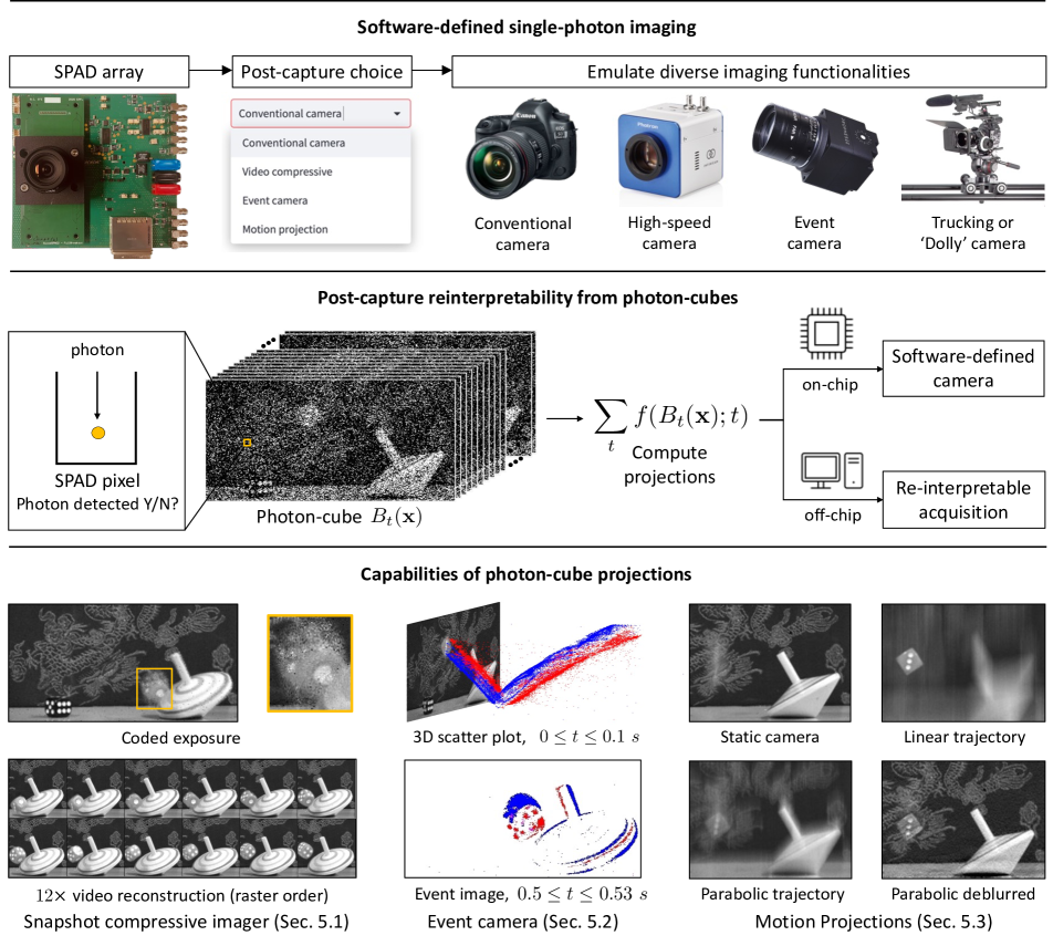
Figure 1: (top) SoDaCam can emulate a variety of cameras from the photon-cubes acquired by single-photon devices. (middle) Photon-cubes represent the spatio-temporal detection of photons as a sequence of binary frames. Projections of the photon-cube, when computed either on or off-chip, result in reinterpretable and software-defined cameras. We demonstrate the versatility of photon-cube projections on a real dynamic scene: a die falls on a table, bounces, spins in the air, and later ricochets off a nearby toy top. (bottom) The cameras emulated by our photon-cube projections can produce a $12\times$ high-speed video from a single compressive snapshot, event-stream representations of two time intervals (blue and red depict positive and negative spikes respectively), an image where the die appears stationary, as well as a motion-deblurred image.

Computing photon-cube projections.

One way to obtain photon-cube projections is to read the entire photon-cube off the SPAD array and then perform relevant computations off-chip; we adopt this strategy for our experiments in Secs. 6.1 and 6.2. While reasonable for certain applications, reading out photon-cubes requires an exorbitant data bandwidth, which can be up to $100$ Gbps for a $1$ MPixel array—well beyond the capacity of existing data peripherals. Such readout considerations will become center stage as large-format SPAD arrays are fabricated [48, 49].

An alternative is to avoid transferring the entire photon-cube by computing projections near sensor. As a proof-of-concept, we implement photon-cube projections on UltraPhase [1], a recently-developed programmable SPAD imager with independent processing cores that have dedicated RAM and instruction memory. We show, in Sec. 6.3, that computing projections on-chip greatly reduces sensor readout and, as a consequence, power consumption.

Implications: Toward a photon-level software-defined camera.

The photon-cube projections introduced in this paper are computational constructs that provide a realization of software-defined cameras or SoDaCam. Being software-defined, SoDaCam can emulate multiple cameras simultaneously without additional hardware complexity. SoDaCam, by going beyond baked-in hardware choices, unlocks hitherto unseen capabilities—such as $2000$ FPS video from $25$ Hz readout (Fig. 7); event imaging in very low-light conditions (Fig. 9); and motion stacks, which are a stack of images wherein each image, objects only in certain velocity ranges appear sharp (Fig. 6).

Limitations.

The SPAD array [19] used in this work has a relatively low spatial resolution ($512\times 256$), and a low fill-factor ($\scriptstyle\sim$$10$%) owing to the lack of microlenses in the prototype used. Similarly, the near-sensor processor that we use has limited capabilities compared to off-chip processors. However, with rapid progress in the development of single-photon cameras [48, 49] and increasing interest in near-sensor processors, we anticipate that many of these shortcomings will be addressed in the upcoming years.

2 Related Work

Reinterpretable imaging

has previously been explored at the granularity of light rays [3], by modulating the plenoptic function, and at the level of spatio-temporal voxels [20], by using fast per-pixel shutters. SoDaCam represents a logical culmination of reinterpretability at the level of photon detections, that facilitates multiple post-capture imaging functionalities.

Programmable imaging

using a digital micromirror device was first introduced in Nayar et al. [51] to perform pre-capture radiometric manipulations. Modern programmable cameras are typically near-sensor processors [8, 69, 71] that can perform limited operations in analog [46, 69, 55], while more complex operations [45, 9] occur after analog-to-digital conversion (ADC). In contrast, by performing post-capture computations directly on photon detections, we can perform complex operations without incurring the read-noise penalty that is associated with ADC.

Passive single-photon imaging.

Only recently have SPADs been utilized as passive imaging devices, with applications in high-dynamic range imaging [29, 30, 37, 50], motion-compensation [31, 58], burst photography [11, 42] and object tracking [22]. Compared to compute-intensive burst-photography methods [11], our proposed techniques involve lightweight computations that can be performed near sensor. These computations can also be performed using other single-photon imagers such as Jots [15, 17], which feature higher sensor resolution and photon-efficiency [40], albeit at lower frame-rates and higher read noise.

Reducing the readout of SPADs.

Several data reduction strategies have been proposed in the context of SPADs that are used to timestamp incident photons, including: coarse histograms [13, 23, 56], compressive histograms [21], and measuring differential time-of-arrivals [77, 70]. When SPADs are operated as photon-detectors, multi-bit counting [48], or summing binary frames, can reduce readout. While compression is not our main objective, we show that photon-cube projections act as camera-specific compression schemes that dramatically reduce sensor readout.

3 Background: Single-Photon Imaging Model

A SPAD array captures incident light as a photon-cube: a temporal sequence of binary frames that represents the pixel-wise detection of photons across their respective exposure windows. We can model the stochastic arrival of photons as a Poisson process [72], allowing us to treat spatio-temporal values of the photon-cube as independent Bernoulli random variables with

$$\text{Pr}\left\{B_{t}(\mathbf{x})=1\right\}=1-e^{-\left(\eta\Phi(\mathbf{x},t)+r_{q}\right)w_{\text{exp}}},$$ (1)

where $B_{t}(\mathbf{x})$ represents the value of the photon-cube at pixel $\mathbf{x}$ and exposure index $1\leq t\leq T$, which receives a mean incident flux of intensity $\Phi(\mathbf{x},t)$ across its exposure of duration $w_{\text{exp}}$. Additionally, $\eta$ is the photon detection efficiency of the SPAD, and $r_{q}$ denotes the sensor’s dark count rate—which is the rate of spurious counts unrelated to incident photons. While individual binary frames are extremely noisy, the temporal sum of the photon-cube

$$\mathcal{I}_{\text{sum}}(\mathbf{x}):=\sum_{t=1}^{T}B_{t}(\mathbf{x}),$$ (2)

can produce an ‘image’ of the scene that is sharp in static regions, but blurry in dynamic regions (Fig. 2 (top)). Indeed, in static regions, the sum-image can be used to derive a maximum likelihood estimator of the scene intensity [4], given by $\hat{\Phi}(\mathbf{x})=-\ln(1-T^{-1}{\mathcal{I}_{\text{sum}}(\mathbf{x})})/{\eta w_{\text{exp}}}-{r_{q}}/{w_{\text{exp}}}$.

4 Projections of the Photon-Cube

The temporal sum described in Eq. 2 is a simple instance of projections of a photon-cube. Our key observation is that it is possible to compute a wide range of photon-cube projections, each of which emulates a unique sensing modality post-capture—including modalities that are difficult to achieve with conventional cameras. For example, varying the number of bit-planes that are summed over emulates exposure bracketing [12, 43], which is typically used for HDR imaging. Compared to conventional exposure bracketing, the emulated exposure stack, being software-defined, does not require spatial and temporal registration, which can often be error-prone. Fig. 2 (top) shows an example of an exposure stack computed from a photon-cube.

Going further, we can gradually increase the complexity of the projections. For example, consider a coded exposure projection that multiplexes bit-planes with a temporal code

$$\mathcal{I}_{\text{flutter}}(\mathbf{x}):=\sum_{t=1}^{T}C_{t}B_{t}(\mathbf{x}),$$ (3)

where $C_{t}$ is the temporal code. An example of globally-coded exposures is the flutter shutter camera [53], which uses pseudo-random binary codes for motion-deblurring.

More general coded exposures can be obtained via spatially-varying temporal coding patterns $C_{t}(\mathbf{x})$:

$$\mathcal{I}_{\text{coded}}(\mathbf{x}):=\sum_{t=1}^{T}C_{t}(\mathbf{x})B_{t}(\mathbf{x}).$$ (4)

Fig. 2 (bottom) shows spatially-varying exposures that use a quad (Bayer-like) spatial pattern and random binary masks. With photon-cubes, we can perform spatially-varying coding without bulky spatial light modulators, similar to focal-plane sensor-processors [46, 69]. Moreover, we can capture multiple coded exposures simultaneously, which is challenging to realize in existing sensors. In Sec. 5.1, we describe coding patterns for video compressive sensing.

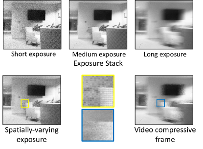
Figure 2: Coded exposures from photon-cubes. (top) An exposure stack with sum-images computed using $250$, $500$, and $1000$ bit-planes. Short exposures are noisy while long exposures exhibit motion blur. (bottom) Spatially-varying exposure that uses a quad pattern [32] (see inset), and a video compressive frame that uses $16$ random binary masks to modulate the photon-cube. Zoom-in to see details.

Spatial and temporal gradients form the building blocks of several computer vision algorithms [7, 24, 26, 39, 11]. Given this, another projection of interest is temporal contrast, i.e., a derivative filter preceded by a smoothing filter:

$$\mathcal{I}_{\text{contrast}}(\mathbf{x},t):=D_{t}\circ G*B_{t}(\mathbf{x}),$$ (5)

where $D_{t}$ is the difference operator, $G$ could be exponential or Gaussian smoothing, $\circ$ denotes function composition, and $*$ denotes convolution. Due to their sparse nature, gradients form the basis of bandwidth- and power-efficient event cameras [36, 60, 14, 6], which we emulate in Sec. 5.2.

So far, we have considered projections taken only along the time axis. Next, we consider a more general class of spatio-temporal projections that lead to novel functionalities. For instance, computing a simple projection, such as the temporal sum, along arbitrary spatio-temporal directions emulates sensor motion during exposure time [33], but without moving the sensor. We achieve this by shifting bit-planes and computing their sum:

$$\mathcal{I}_{\text{shift}}(\mathbf{x}):=\sum_{t=1}^{T}B_{t}\left(\mathbf{x}+\mathbf{r}(t)\right),$$ (6)

where $\mathbf{r}$ is a discretized 2D trajectory that determines sensor motion. Outside a software-defined framework, such projections are hard to realize without physical actuators. We describe the capabilities of motion projections in Sec. 5.3.

In summary, the proposed photon-cube projections are simple linear and shift operators that lead to a diverse set of post-capture imaging functionalities. These projections pave the way for future ‘swiss-army-knife’ imaging systems that achieve multiple functionalities (e.g., event cameras, high-speed cameras, conventional cameras, HDR cameras) simultaneously with a single sensor. Finally, these projections can be computed efficiently in an online manner, which makes on-chip implementation viable (Sec. 6.3).

At this point, we note that a key enabling factor of photon-cube projections is the extremely high temporal-sampling rate of SPADs. Indeed, the temporal sampling rate determines key aspects of sensor emulation, such as the discretization of temporal derivatives and motion trajectories. This raises a natural question: can we use conventional high-speed cameras for computing projections?

Trade-off between frame-rate and SNR.

In principle, photon-cube projections can be computed using regular (CMOS or CCD based) high-speed cameras. Unfortunately, each frame captured by a high-speed camera incurs a read-noise penalty, which increases with the camera’s frame-rate [6]. In fact, the read noise levels of high-speed cameras [1] can be $10$–$30\times$ higher than consumer cameras [28]. Coupled with the low per-frame incident flux at high frame-rates, high levels of read noise result in extremely low SNRs. In contrast, SPADs do not incur a per-frame read noise and are limited only by the fundamental photon noise. Hence, for the post-capture software-defined functionalities proposed here, it is imperative to use SPADs.

5 Emulating Cameras from Photon-Cubes

Sec. 4 presented the concept of photon-cube projections and its potential for achieving multiple post-capture imaging functionalities. As case studies, we now demonstrate three imaging modalities: video compressive sensing, event cameras, and motion-projection cameras. These modalities have been well-studied over several years; in particular, there exist active research communities around video compressive sensing and event cameras today. We also show new variants of these imaging systems that arise from the software-defined nature of photon-cube projections.

5.1 Video Compressive Sensing

Video compressive systems optically multiplex light with random binary masks, such as the patterns in Fig. 3 (left). As discussed in the previous section, such multiplexing can be achieved computationally using photon-cubes.

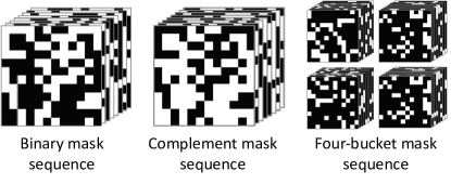
Figure 3: Modulating masks for video compressive sensing. (left) A single VCS measurement temporally compresses a sequence of frames using binary random masks. (center) Two-bucket cameras capture an additional measurement by using the complementary mask sequence. (right) We propose using multi-bucket captures by randomly choosing an active bucket for each frame. Both two-bucket and multi-bucket captures have $100$% light efficiency. All masks are visualized here for $16\times 16$ pixels.

Two-bucket cameras.

One drawback of capturing coded measurements is the light loss due to blocking of incident light. To prevent loss of light, coded two-bucket cameras [69] capture an additional measurement that is modulated by the complementary mask sequence (Fig. 3 (center)). Such measurements recover higher quality frames, even after accounting for the extra readout [9, 14]. Two-bucket captures can be readily derived from photon-cubes, by implementing Eq. 4 with the additional mask sequence.

Multi-bucket cameras.

We can extend the idea of two-bucket captures to multi-bucket captures by accumulating bit-planes in one of $k$ buckets that is randomly chosen at each time instant and pixel location. Since multiplexing is performed computationally, we do not face any loss in photoreceptive area that [59, 68] hampers existing multi-bucket sensors. Multi-bucket captures can reconstruct a large number of frames by better conditioning video recovery and provide extreme high-speed video imaging. Fig. 3 (right) shows the modulating masks for a four-bucket capture.

5.2 Event Cameras

Next, we describe the emulation of event cameras, which capture changes in light intensity and are conceptually similar to the temporal contrast projection introduced in Eq. 5. Physical implementations of event sensors [36, 60, 14, 6] generate a photoreceptor voltage $V(\mathbf{x},t)$ with a logarithmic response to incident flux $\Phi(\mathbf{x},t)$, and output an event $(\mathbf{x},t,p)$ when this voltage deviates sufficiently from a reference voltage $V_{\text{ref}}(\mathbf{x})$:

$$|V(\mathbf{x},t)-V_{\text{ref}}(\mathbf{x})|>\tau,$$ (7)

where $\tau$ is called the contrast-threshold and $p=\text{sign}(V(\mathbf{x},t)-V_{\text{ref}}(\mathbf{x}))$ encodes the polarity of the event. Once an event is generated, $V_{\text{ref}}(\mathbf{x})$ is updated to $V(\mathbf{x},t)$. Eq. 7, for a smoothly-varying flux intensity, thresholds a function of the temporal gradient, i.e., $\partial_{t}\log(\Phi(\mathbf{x},t))$.

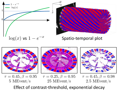
Figure 4: Event stream from photon-cubes. (top left) By exploiting the non-linear response curve of SPADs to encode brightness, we can avoid the underflow issues of a log-response. We visualize events generated from photon-cubes using a $3$D scatter plot of polarities (top right, $14000$ bit-planes), and frame accumulation of events (bottom, $1200$ bit-planes). Blue and red denote positive and negative spikes respectively. The event images also show the effect of varying the contrast threshold $\tau$ and exponential decay $\beta$—larger values yield a less noisy but sparser event stream.

From bit-planes to event streams.

To produce events from SPAD frames, we compute an exponential moving average (EMA) of the bit-planes, as $\mu_{t}(\mathbf{x})=(1-\beta)B_{t}(\mathbf{x})+\beta\mu_{t-1}(\mathbf{x})$—where $\mu_{t}(\mathbf{x})$ is the EMA, $\beta$ is the smoothing factor, and $B_{t}$ is a bit-plane. We generate an event when $\mu_{t}(\mathbf{x})$ deviates from $\mu_{\text{ref}}(\mathbf{x})$ by at least $\tau$:

$$|h(\mu_{t}(\mathbf{x}))-h(\mu_{\text{ref}}(\mathbf{x}))|>\tau,$$ (8)

where $h$ is a scalar function applied to the EMA. We can see that Eq. 8 thresholds temporal contrast, by observing the role played by the EMA and the difference operator.

Setting $h$ to be the logarithm of the flux MLE mimics Eq. 7. However, since the log-scale is used to prevent sensor saturation, a simpler alternative is to use the non-saturating response curve of SPAD pixels ($h(x)=x$). The response curve takes the form of $1-\exp\left(-\alpha\Phi(\mathbf{x},t)\right)$, where $\alpha$ is a flux-independent constant. As a major advantage, this response curve avoids the underflow issues of the log function that can occur in low-light scenarios [62].

The SPAD’s frame rate determines the time-stamp resolution of emulated events. In Fig. 4, we show the events generated from a photon-cube acquired at a frame-rate of $96.8$ kHz—resulting in a time-stamp resolution of ${\raise 0.73193pt\hbox{$\scriptstyle\sim$}}10$ $\mu\text{s}$ that is comparable to those of existing event cameras.

Figure 5: Motion projections. (top) Integrating along a linear trajectory in the photon-cube changes the apparent image-space velocity of scene objects. Details are seen for (top left) the case when static, and (top right) the metallic tape when the sensor translates along the $x$-axis. (bottom) A parabolic integration trajectory results in a motion-invariant image, resulting in similar blur kernels for all objects. (bottom right) Deblurring with the resultant shift-invariant point spread function (shown in inset) produces a sharp image.

How do SPAD-events differ from the output of a regular event camera?

The main difference is the expression of temporal contrast, given by $\partial_{t}h$, is now $-\partial_{t}\exp({-\alpha\Phi(\mathbf{x},t)})$, instead of $\partial_{t}\log(\Phi(\mathbf{x},t))$. This difference poses no compatibility issues for a large class of event-vision algorithms that utilize a grid of events [13, 57, 66] or brightness changes [18]. We show examples of downstream applications using SPAD-events in Suppl. Sec. 2. Finally, SPAD-events can be easily augmented with spatially- and temporally-aligned intensity information—a synergistic combination that has been exploited by several recent event-vision works [18, 25, 74].

5.3 Motion Projections

Having described the emulation of cameras that capture coded exposures and temporal contrasts, we now shift our attention to cameras that emulate sensor motion during exposure, viz. motion cameras. We describe two useful trajectories when emulating motion cameras using Eq. 6.

Linear trajectory.

The simplest sensor trajectory involves linear motion, where $\mathbf{r}(t)=(bt+c)\,\mathbf{\hat{p}}$ for some constants $b,c\in\mathbb{R}$ and unit vector $\mathbf{\hat{p}}$. As Fig. 5 (top row) shows, this can change the scene’s frame of reference: making moving objects appear stationary and vice-versa.

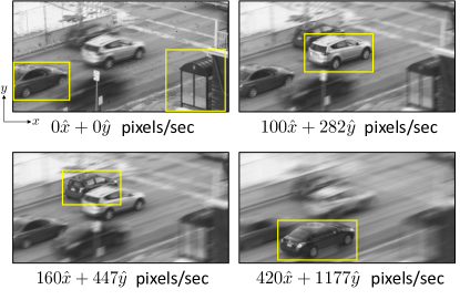
Figure 6: Motion stack. Computing multiple linear projections with different trajectories can produce a stack of images where objects with matching velocities are sharp. Here, we show a traffic scene involving four cars that have four different velocities. By suitably altering the slope of the linear trajectory, we can produce images where only one of the cars appears sharp at a time. We indicate the slope of the trajectories chosen and the objects that are “in-focus”.

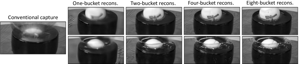
Figure 7: High-speed videography at $2000$ FPS of a tennis ball dropped into a bowl of water, from a $25$ Hz readout. The conventional capture provides a visualization of the scene dynamics. It is challenging to reconstruct a large number of frames from a single compressive snapshot. Multi-bucket captures recover frames with significantly greater detail, such as the crown of water surrounding the ball. We include more sequences (e.g., a bursting balloon) in the supplementary material.

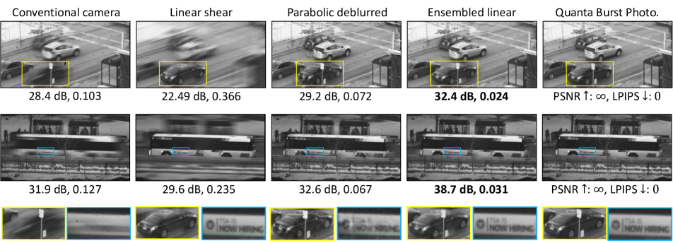
Figure 8: Deblurring of traffic scenes using motion projections. Linear projections can recover details of moving objects if their velocity is known. When only the motion direction is known (e.g., road’s orientation), a sharp image can be obtained by either deblurring a parabolic projection or by blending multiple randomly-sampled linear projections. We quantitatively compare against the compute- and bandwidth-expensive Quanta Burst Photography [11], based on PSNR and LPIPS [76].

Motion-invariant parabolic projection.

If motion is along $\mathbf{\hat{p}}$, parabolic integration produces a motion-invariant image [33]—all objects, irrespective of their velocity, are blurred by the same point spread function (PSF), up to a linear shift. Thus, a deblurred parabolic capture produces a sharp image of all velocity groups (Fig. 5 (bottom row)). The parabolic trajectory is given by $\mathbf{r}(t)=(at^{2}+bt+c)\,\mathbf{\hat{p}}$. We choose $a$ based on the maximum object velocity and $b,c$ so the parabola’s vertex lies at $T/2$. We readily obtain the PSF by applying the parabolic integration to a delta input. Upon deconvolution using the PSF, a parabolic projection provides the optimal SNR for a blur-free image from single capture when only the direction of velocity is known.

Ensembling linear projections.

Finally, we leverage the flexibility of photon-cubes to compute multiple linear projections, as seen in Fig. 6. This produces a stack of images where one velocity group is motion-blur free at a time—or a ‘motion stack’, analogous to a focal stack. This novel construct can be used to compensate motion by blending stack images using cues such as blur orientation or optical flow.

6 Hardware and Experimental Results

We design a range of experiments to demonstrate the versatility of photon-cube projections: both when computations occur after readout (Secs. 6.2 and 6.1), and when they are performed near-sensor on-chip (Sec. 6.3). All photon-cubes were acquired using the SwissSPAD2 array [19], operated using one of two sub-arrays, each having $512\times 256$ pixels, and at a frame-rate of $96.8$ kHz. For the on-chip experiments, we use the UltraPhase compute architecture to interface with photon-cubes acquired by the SwissSPAD2.

6.1 SoDaCam Capabilities

High-speed compressive imaging.

We reconstruct $80$ frames from compressive snapshots that are emulated at $25$ Hz, resulting in a $2000$ FPS video. We decode compressive snapshots using a plug-and-play (PnP) approach, PnP-FastDVDNet [26]. As Fig. 7 shows, it is challenging to recover a large number of frames from a single compressive measurement. Using the proposed multi-bucket scheme significantly improves the quality of video reconstruction. While multi-bucket captures require more bandwidth, this can be partially amortized by coding only dynamic regions, which we show in Suppl. Sec. 1.

Motion projections on a traffic scene.

Fig. 8 shows two traffic scenes captured using a $50$ mm focal length lens and at $30$ Hz emulation. When object velocity is known, a linear projection can make moving objects appear stationary. If only the velocity direction is known (e.g., road’s orientation in Fig. 8), a parabolic projection provides a sharp reconstruction of all objects. We deblur parabolic captures using PnP-DnCNN [75]. We offer an improvement by randomly sampling $8$ linear projections along the velocity direction and blending them using the optical flow predicted by RAFT [17] between two short exposures.

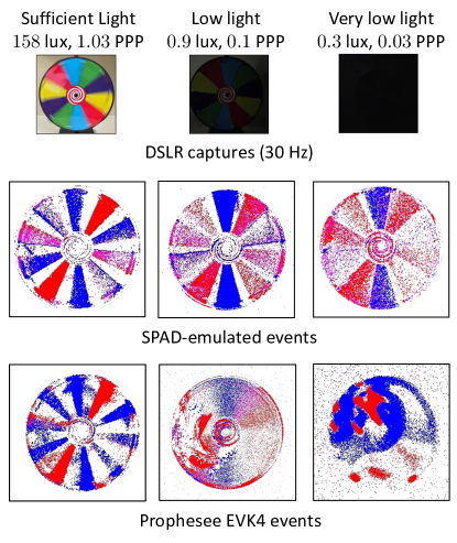
Figure 9: Comparison to a state-of-the-art event camera. SPAD-events can capture temporal gradients even when the light-level is reduced by $500\times$, by benefiting from their single-photon sensitivity and bounded brightness response curve. In contrast, low-light induces blur and deteriorates the Prophesee’s event stream. As a measure of the light-level, we report the PPP (photons per pixel) averaged across bit-planes and a light meter’s reading at the sensor location.

Low-light event imaging.

Fig. 9 compares event-image visualizations of SPAD and that of a state-of-the-art commercial event sensor (Prophesee EVK4), across various light levels, with an accumulation period of $33$ ms. For a fair comparison, we bin the Prophesee’s events in blocks of $2\times 2$ pixels and use a smaller aperture to account for the lower fill factor of the SPAD. We tuned event-generation parameters (contrast threshold, integrator decay rate) of both cameras at each light level. Low light induces blur and deteriorates the Prophesee’s event stream. In contrast, SPAD-events continue to capture temporal gradients, due to the SPAD’s low-light capabilities and its brightness-encoding response curve. We include an ablative study of brightness-encoding functions in Suppl. Sec. 2.

Our observations are in concurrence with recent works that examine the low-light performance of event cameras [27, 19], and show that SPAD-events can provide neuromorphic vision in these challenging-SNR scenarios.

6.2 Comparison to High-Speed Cameras

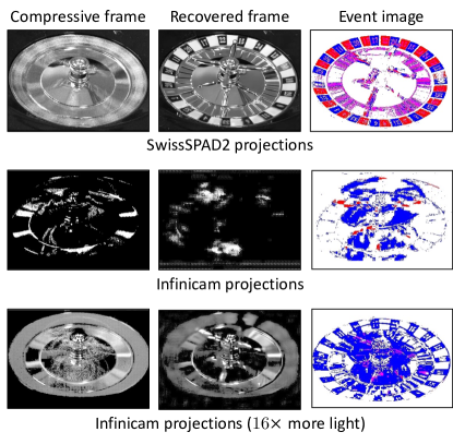
Figure 10: Comparison against conventional high-speed acquisition at $4000$ Hz. (top) SPAD projections recover a $16\times$ compressive video and an event image of a spinning roulette wheel. (middle) Read-noise corrupts the incident flux in the Infinicam high-speed camera, removing details in frames which are compressed on-the-fly. (bottom) Although using a larger aperture to admit more light recovers some detail, noise and compression artifacts still persist.

Recall, as previously discussed in Sec. 4, that read-noise limits the per-frame SNR of high-speed cameras. To demonstrate this limitation, we compute projections using the $4$ kHz acquisition of the Photron Infinicam, a conventional high-speed camera, at a resolution of $1246\times 240$ pixels. We operate the SwissSPAD2 and the Infinicam at ambient light conditions using the same lens specifications. As Fig. 10 shows, read noise corrupts the incident signal in Infinicam and makes it impossible to derive any useful projections. The read noise could be averaged out to some extent if the Infinicam did not perform compression-on-the-fly, but compression is central to the camera’s working and enables readout over USB. Using a larger aperture to admit more light improves the quality of computed projections, but the video reconstruction and event image remain considerably worse than the corresponding outputs of the SPAD.

6.3 Bandwidth and Power Implications

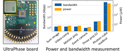
Figure 11: Power and bandwidth requirements when computing photon-cube projections on UltraPhase [1] (left), a recent compute architecture designed for single-photon imaging, at $40$ Hz readout. (right) Our projections act as a compression scheme for photon-cubes, resulting in dramatically reduced sensor readout and power consumption.

While Sec. 6.1 has demonstrated the capabilities of photon-cube projections, we now show that our projections can also be obtained in a bandwidth-efficient manner via near-sensor computations. We implement photon-cube projections on UltraPhase (Fig. 11 (left)), a novel compute architecture designed for single-photon imaging. UltraPhase consists of $3\times 6$ processing cores, each of which interfaces with $4\times 4$ pixels, and can be 3D stacked beneath a SPAD array. We include visualizations and programming details of a few example projections in Suppl. Sec. 5.

We measure the readout and power consumption of UltraPhase when computing projections on $2500$ bit-planes of the falling die sequence (Fig. 1). The projections include: VCS with $16$ random binary masks, an event camera, a linear projection, and a combination of the three. We output projections at $12$-bit depth and calculate metrics based on the clock cycles required for both compute and readout. As seen in Fig. 11 (right), computing projections on-chip dramatically reduces sensor readout and power consumption as compared to reading out the photon-cube. Finally, similar to existing event cameras, SPAD-events have a resource footprint that reflects the underlying scene dynamics.

In summary, our on-chip experiments show that performing computations near-sensor can increase the viability of single-photon imaging in resource-constrained settings.

7 Discussion and Future Outlook

SoDaCam provides a realization of reinterpretable software-defined cameras [51, 20, 3, 2, 34] at the fine temporal resolution of SPAD-acquired photon-cubes. The proposed computations, or photon-cube projections, can match and in some cases, surpass the capabilities of existing imaging systems. The software-defined nature of photon-cube projections provides functionalities that may be difficult to achieve in conventional sensors. These projections can reduce the readout and power-consumption of SPAD arrays and potentially spur widespread adoption of single-photon imaging in the consumer domain. Finally, future chip-to-chip communication standards may also make it feasible to compute projections on a camera image signal processor.

Adding color to SoDaCam.

One way to add color is by overlaying color filter arrays (CFAs) and perform demosaicing on the computed photon-cube projection: depending on the projection, demosaicing could be relatively simple or more complex. As a reference, Bayer CFAs have been considered in the context of both video compressive sensing [26] and event cameras [64]. Incorporating CFAs with motion projections requires careful considerations, e.g., avoiding integrating across pixel locations of differing color.

Future outlook on SPAD characteristics.

A key SPAD characteristic that determines several properties of emulated cameras is the frame rate. While no fundamental limitations prevent SPADs from being operated at the frame rates utilized in this work (${\raise 0.73193pt\hbox{$\scriptstyle\sim$}}100$ kHz), sensor readout and power constraints can preclude high speeds, especially in high-resolution SPAD arrays. Photon-cube projections can enable future large-format SPADs to preserve high-speed information with modest resource requirements.

A platform for comparing cameras.

Comparing imaging modalities can be quite challenging since hardware realizations of sensors can differ in numerous aspects, such as their quantum efficiency, fill factor, pixel pitch, and array resolution. By emulating their imaging models, SoDaCam can serve as a platform for hardware-agnostic comparisons; for instance, determining operating conditions where one imaging modality is advantageous over another.

A Cambrian explosion of new cameras.

Besides comparing cameras, by virtue of being software-defined, SoDaCam can also make it significantly easier to prototype and deploy new unconventional imaging models, and even facilitate sensor-in-the-loop optimization [63, 47, 44] by tailoring photon-cube projections for downstream computer-vision tasks. This is an exciting future line of research.

Supplementary Material for “SoDaCam: Software-defined Cameras via Single-Photon Imaging”

1 Video Compressive Sensing

In this supplementary note, we provide the pseudo code that describes the emulation of two- and multi-bucket cameras and mathematically describe their multiplexing masks. We also specify algorithmic details for video recovery from compressive measurements.

Multi-Bucket Capture Pseudocode

Algorithm 1 describes the emulation of $J$-bucket captures, denoted as $\mathcal{I}_{\text{coded}}^{j}(\mathbf{x})$, from the photon-cube $B_{t}(\mathbf{x})$ using multiplexing codes $C^{j}_{t}(\mathbf{x})$, where $1\leq j\leq J$. Both single compressive snapshots (or one-bucket captures) and two-bucket captures can be emulated as special cases of Algorithm 1, with $J=1$ and $J=2$ respectively.

Algorithm 1 Multi-Bucket Capture Emulation

Photon-cube $B_{t}(\mathbf{x})$

Number of buckets $J$

Multiplexing code for $j$^th bucket, $1\leq j\leq J$, $C_{t}^{j}(\mathbf{x})$

Pixel locations $\mathcal{X}$

Total bit-planes $T$

Multiplexed captures $\mathcal{I}_{\text{coded}}^{j}(\mathbf{x})$

function MultiBucketEmulation($B_{t}(\mathbf{x})$, $C_{t}^{j}(\mathbf{x})$)

     $Y^{j}(\mathbf{x})\leftarrow 0,\,\forall\,j$

     for $\mathbf{x}\in\mathcal{X}$, $1\ \leq j\leq J$ do

         for $1\leq t\leq T$ do

              $\mathcal{I}_{\text{coded}}^{j}(\mathbf{x})\leftarrow\mathcal{I}_{\text{coded}}^{j}(\mathbf{x})+B_{t}(\mathbf{x})\cdot C_{t}^{j}(\mathbf{x})$

         end for

     end for

return $\mathcal{I}_{\text{coded}}^{j}(\mathbf{x})$

end function

Mask sequences for video compressive sensing.

For a single compressive capture ($J=1$), a sequence of binary random is used, i.e, $C^{1}_{t}(\mathbf{x})=1$ with probability $0.5$. For a two bucket capture, we use

$$C^{2}_{t}(\mathbf{x})=1-C^{1}_{t}(\mathbf{x}),$$

which is the complementary mask sequence. For $J>2$, at each timestep $t$ and pixel location $\mathbf{x}$, the active bucket is chosen at random:

$$C^{j}_{t}(\mathbf{x})\leftarrow 1,\;j\sim\text{Uniform}(1,J).$$

This is a direct generalization of the masking used for both one- and two-bucket captures.

Decoding Video Compressive Captures

A variety of decoding algorithms have been developed for video compressive sensing, including: (a) optimization frameworks tailored to the forward model of Eq. 4 and with additional regularization [10, 24], (b) end-to-end deep-learning methods that utilize a large corpus of training data [7, 14, 22, 23, 9], and (c) hybrid, plug-and-play (PnP) approaches that utilize an optimization framework but perform one or more steps using a deep denoiser [5, 20, 26]. We opt to use the PnP approach featuring an ADMM formulation [25] and a deep video denoiser (FastDVDNet [16]) in this work. We justify our choice by noting that PnP-ADMM can produce high-quality reconstructions, comparable to end-to-end counterparts while using an off-the-shelf denoiser—precluding the need to train separate models for various masking strategies.

For computational efficiency, PnP-ADMM requires the gram matrix of the resulting linear forward model of Eq. 4 to be efficiently invertible. The multi-bucket scheme described above adheres to this consideration.

Constant-Bandwidth Comparison

We now present a comparison of single-, two- and multi-bucket compressive captures when the readout rate is fixed. As Supp. Fig. 1 shows, multi-bucket captures provide higher fidelity reconstructions even when bandwidth is fixed. Furthermore, their bandwidth cost can be amortized, to some extent, by coding only dynamic regions—we describe this next.

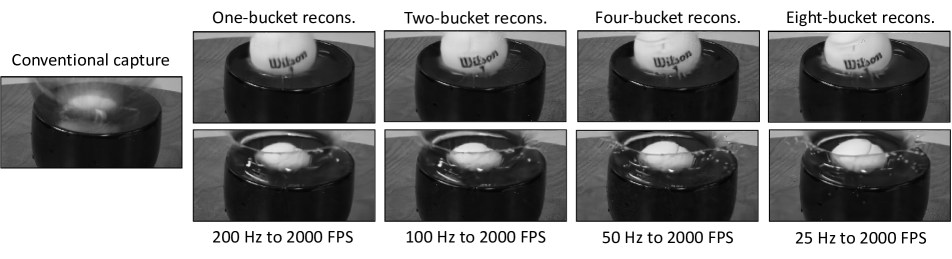
Supplementary Figure 1: Fixed readout comparison of compressive video schemes. We compare video reconstruction obtained from a single compressive snapshot, two-bucket capture, four-bucket capture and eight-bucket capture while holding readout constant—we achieve this by commesurately increasing readout, for instance, by reading out single compressive snapshots at $200$ Hz. We indicate the readout rate here in Hertz (Hz) and the frame-rate of the reconstructed video in FPS. Clearly, multi-bucket captures provide better reconstruction results than a burst of independently multiplexed captures.

Coding Only Dynamic Regions: Mitigating the Bandwidth Cost of Multi-Bucket Captures

We observe that multi-bucket captures capture redundant information in static regions of the scene since each pixel in a static region has the same expected value under random binary modulation. Hence, we propose coding only dynamic regions—the dynamic region-of-interest (RoI) can be determined by masking pixels whose coded exposures deviate significantly from one another. As seen in Supp. Fig. 2, the dynamic content may just be $25$% of the image area, which provides significant scope for bandwidth savings. We observe that we can code just $25$% of the total pixels, among additional compressive measurements, without a perceptible drop in visual quality, which yields an overall bandwidth requirement of $1.45\times$, or under twice the bandwidth cost of a single compressive measurement.

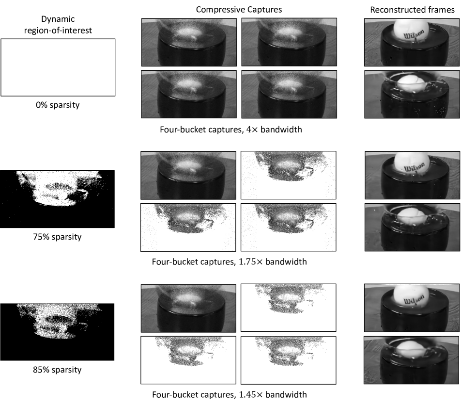
Supplementary Figure 2: Coding dynamic regions can reduce readout of multi-bucket captures. (left column) Dynamic regions are detected by computing the standard deviation of the coded exposures and thresholding them appropriately (e.g., by the $75^{\text{th}}$ percentile)—we show the dynamic regions in white here. Coded exposures are transmitted only in the dynamic regions. For the static regions, we simply use a long exposure—by adding multi-bucket captures. (right column) We observe that readout-bandwidth can be reduced to $1.75\times$ from $4\times$ in the case of a four-bucket capture with no perceptual degradation of reconstruction quality. Bandwidth is provided here as a multiple of the readout of a single compressive capture.

Results on More Sequences

Additional results are shown in Supp. Fig. 3.

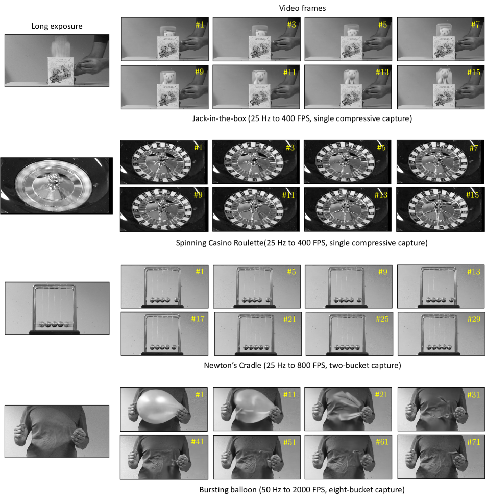
Supplementary Figure 3: Results on additional sequences. We use Hertz (Hz) to indicate the rate of emulation and frames-per-second (FPS) to indicate the frame-rate of the reconstructed video. Frame numbers are indicated in yellow font.

2 Event Cameras

Event-Generation Pseudocode

We provide the pseudocode for emulating events from photon-cubes in Algorithm 2. The contrast threshold $\tau$ and exponential smoothing factor $\beta$ are the two parameters that determine the characteristics of the resulting event stream, such as its event rate (number of events per second). We use an initial time-interval $T_{0}$ (typically $80$–$100$ bit-planes) to initialize the reference moving average, with $T_{0}$ being much smaller than $T$. The result of this pseudocode is an event-cube, $E_{t}(\mathbf{x})$, which is a sparse spatio-temporal grid of event polarities—positive spikes are denoted by $1$ and negative spikes by $-1$. From the emulated event-cube, other event representations can be computed such as: an event stream, $\{(\mathbf{x},t,p)\}$, where $p\in\{-1,1\}$ indicates the polarity of the event; a frame of accumulated events [12] (seen in Figs. 4 and 9); and a voxel grid representation [27], where events are binned into a few temporal bins (shown in Supp. Fig. 4 (top left) using $3$ temporal bins).

Algorithm 2 Event Camera Emulation

Photon-cube $B_{t}(\mathbf{x})$

Contrast threshold $\tau$

Exponential smoothing factor, $\beta$

Pixel locations $\mathcal{X}$

Initial time-interval $T_{0}$, for computing reference moving average

Total bit-planes $T$

Event-cube $E_{t}(\mathbf{x})$ that describes the spatio-temporal spikes

function EventCameraEmulation($B_{t}(\mathbf{x})$, $\tau$, $\beta$, $T_{0}$)

     $E_{t}(\mathbf{x})\leftarrow 0,\,\forall\,t,\,\forall\,\mathbf{x}$

     for $\mathbf{x}\in\mathcal{X}$ do

         Reference moving average, $\mu_{\text{ref}}(\mathbf{x})\leftarrow 0$

         Current moving average, $\mu_{0}(\mathbf{x})\leftarrow 0$

         for $1\leq t\leq T_{0}$ do

              $\mu_{\text{ref}}(\mathbf{x})\leftarrow\beta\mu_{\text{ref}}(\mathbf{x})+(1-\beta)B_{t}(\mathbf{x})$

         end for

         for $T_{0}\leq t\leq T$ do

              $\mu_{t}(\mathbf{x})\leftarrow\beta\mu_{t-1}(\mathbf{x})+(1-\beta)B_{t}(\mathbf{x})$

              if $\left\lvert\mu_{t}(\mathbf{x})-\mu_{\text{ref}}(\mathbf{x})\right\rvert>\tau$ then

                  $E_{t}(\mathbf{x})\leftarrow\text{sign}(\mu_{t}(\mathbf{x})-\mu_{\text{ref}}(\mathbf{x}))$

                  $\mu_{\text{ref}}(\mathbf{x})\leftarrow\mu_{\text{ref}}(\mathbf{x})+\tau*\text{sign}(\mu_{t}(\mathbf{x})-\mu_{\text{ref}}(\mathbf{x}))$

              end if

         end for

     end for

return $E_{t}(\mathbf{x})$

end function

Compatibility of SPAD-Events with Existing Event-Vision Algorithms

We now provide examples of downstream algorithms applied to SPAD-events, which shows the compatibility of the emulated event streams with existing event-vision algorithms. Supplementary Figure 4 shows three downstream algorithms with SPAD-events as their input: Contrast Maximization [8] which generates a warped image of events that has sharp edges (top right), E2VID [13] which estimates intensity frames from an event stream (bottom left), and DCEIFlow [21] which computes dense optical flow using intensity frames and aligned events (bottom right). Both E2VID and DCEIFlow use a voxel grid representation of events as their inputs. We include the visualization of a voxel grid representation in Supp. Fig. 4 (top left). All event streams were emulated using $3000$ bit-planes of photon-cubes acquired at $96.8$ kHz, and using $\beta=0.95$ and $\tau=0.4$ as emulation parameters. We note that the performance of these algorithms can be improved by finetuning pre-trained learning-based models on a dataset of SPAD-events.

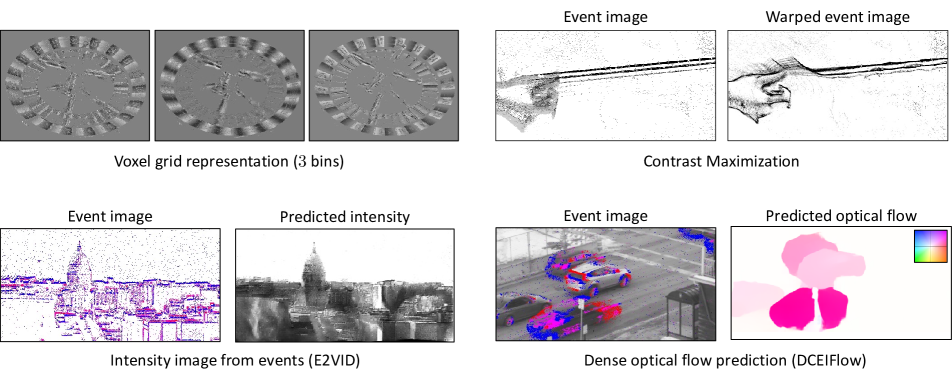
Supplementary Figure 4: Compatibility of SPAD-events with existing event-vision algorithms. The flow field visualization follows Baker et al. [2]. The photon-cube for the contrast maximization output was obtained from Ma et al. [11].

Ablation of Brightness-Encoding Functions

Our event emulation scheme (Algorithm 2) relies on the SPAD’s response curve to encode scene brightness, which is a non-linear and non-saturating response of the form

$$1-\exp(-\alpha\Phi(\mathbf{x},t)),$$

where $\alpha=\eta t_{\text{exp}}$ and assuming negligible dark count rate (DCR). Current event cameras typically use a logarithmic response to encode scene brightness. This can also be utilized to emulate events from photon-cubes by setting $h$ (as described in Eq. 8) to be the log-MLE function:

$$h(\mu)=\log\left(-\frac{\log(1-\mu)}{\eta t_{\text{exp}}}\right).$$

However, a log-response suffers from underflow issues, particularly at low-light scenarios as seen in Supp. Fig. 5.

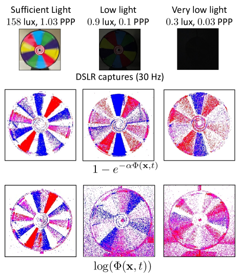
Supplementary Figure 5: Comparison of brightness encoding functions. While the log-MLE is comparable to using the SPAD’s response curve at ambient light levels, at low flux levels the underflow issues associated with the log function occur. Here, $\alpha$ denotes a sensor-determined and flux-independent constant.

SoDaCam Flexibility and SPAD-Events

Here are a few benefits of the SoDaCam approach for event-based imaging:

• Direct access to intensity information. By computing a sum image, SoDaCam makes intensity frames that are spatially- and temporally-aligned with the generated event stream available. This precludes the need for multiple devices, which often require careful alignment and calibration.

• Further, the intensity frames obtained via the sum-image feature the SPAD’s imaging capabilities, i.e., such intensity frames feature a high dynamic range and can be utilized in low-light imaging scenarios. This is in contrast to dynamic active vision sensors (DAVIS) [3, 6], where a conventional frame, which has limited dynamic range and low-light capabilities compared to SPAD-derived images, can be obtained in addition to the event stream.

• Computing multiple event-streams simultaneously. Contrast threshold $\tau$ is an important parameter that controls the sparsity and noise level of generated event stream: small values of $\tau$ can produce potentially noisy event streams that require extensive processing, while large values of $\tau$ can result in very sparse streams with less useful information. With SoDaCam, it is possible to emulate event streams with different values of $\tau$ simultaneously, thereby amortizing these trade-offs. In fact, this can be thought of as analogous to exposure stacks but in the context of event-imaging. Supplementary Figure 6 (top row) shows an example of an ‘event-image stack’.

• Per-pixel contrast thresholds. We can also vary the contrast threshold $\tau$ as a function of pixel location or incident intensity. For instance, we can use a smaller contrast threshold if we have an estimate of the incident intensity with less variance and a higher contrast threshold when there is more variance. We show an example of this in Supp. Fig. 4 (bottom right), where we vary the contrast threshold between $0.35$ and $0.45$ as a linear function of the sample variance of the moving average, $\mu_{t}(\mathbf{x})$.

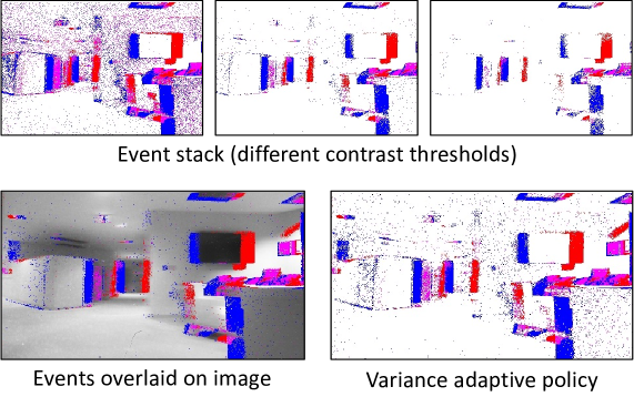
Supplementary Figure 6: Flexible event-based imaging. (top) An ‘event-stack’ that employs increasing contrast thresholds, $\tau=0.35,0.4,0.45$. (bottom) We can also output frames with aligned events, and use event generation policies that may not be trivial to realize in hardware—such as varying the contrast threshold $\tau$ as a linear function of the sample variance.

3 Motion Projections

Pseudocode for Emulating Motion Cameras

Algorithm 3 provides the pseudocode for emulating sensor motion from a photon-cube, where the sensor’s trajectory is determined by the discretized function $\mathbf{r}$. At each time instant $t$, we shift bit-planes by $\mathbf{r}(t)$ and accumulate them in $\mathcal{I}_{\text{shift}}$. For pixels that are out-of-bounds, no accumulation is performed. For this reason, the number of summations that occur varies spatially across pixel locations $\mathbf{x}$—we normalize the emulated shift-image by the number of pixel-wise accumulations $N(\mathbf{x})$ to account for this. The function $\mathbf{r}$ can be obtained by discretizing any smooth $2$D trajectory: by either rounding up or dithering, or by using a discrete line-drawing algorithm [4].

Algorithm 3 Motion Camera Emulation

Photon-cube $B_{t}(\mathbf{x})$

Discretized trajectory $\mathbf{r}(t)$

Pixel locations $\mathcal{X}$

Total bit-planes $T$

$\mathcal{I}_{\text{shift}}(\mathbf{x})$

function MotionCameraEmulation($B_{t}(\mathbf{x})$, $\mathbf{r}$)

     $\mathcal{I}_{\text{shift}}(\mathbf{x})\leftarrow 0,\,\forall\,\mathbf{x}$

     for $\mathbf{x}\in\mathcal{X}$ do

         Normalizer, $N(\mathbf{x})\leftarrow 0$

         for $1\leq t\leq T$ do

              if $\mathbf{x}+\mathbf{r}(t)\in\mathcal{X}$ then

                  $N(\mathbf{x})\leftarrow N(\mathbf{x})+1$

                  $\mathcal{I}_{\text{shift}}(\mathbf{x})\leftarrow\mathcal{I}_{\text{shift}}(\mathbf{x})+B_{t}(\mathbf{x}+\mathbf{r}(t))$

              end if

         end for

         if $N(\mathbf{x})>0$ then

              $\mathcal{I}_{\text{shift}}(\mathbf{x})\leftarrow\mathcal{I}_{\text{shift}}(\mathbf{x})/N(\mathbf{x})$

         end if

     end for

return $\mathcal{I}_{\text{shift}}(\mathbf{x})$

end function

As described in Sec. 5.3, we consider two trajectories: linear and parabolic. Linear trajectories are parameterized by their slope

$$\mathbf{r}(t)=v\left(t-\frac{T}{2}\right)\mathbf{\hat{p}},$$

where $v$ is the object velocity, $\mathbf{\hat{p}}$ is a unit vector that describes the trajectory’s direction, and $T$ is the total number of bit-planes. Parabolic trajectories are parameterized by their maximum absolute slope, $v_{\text{max}}$

$$\mathbf{r}(t)=\frac{v_{\text{max}}}{T}\left(t-\frac{T}{2}\right)^{2}\mathbf{\hat{p}}.$$

To prevent tail-clipping, which are image artifacts introduced by the finite extent of the parabolic integration, it is important to choose $v_{\text{max}}$ to be sufficiently higher than the velocity of objects in the scene. Both linear and parabolic trajectories have a zero at $t=T/2$—which allows blending multiple linear projections without any pixel alignment issues.

Blending Multiple Linear Projections

As shown in Fig. 8, randomly sampling multiple linear projections (seen in Supp. Fig. 7 (left column)) can provide motion compensation when only the motion direction, and not the exact extent of motion, is known. To blend these projections, in addition to the randomly sampled linear projections, we also compute two short exposures using bit-planes at the beginning and end of the photon-cube. For the scenes shown in Fig. 8, we used the first $200$ and the last $200$ bit-planes to emulate short exposures. We then use RAFT [17] to predict optical flow between the two short exposures—which can be used to select the linear projection that can best compensate motion as a function of the pixel location (as seen in Supp. Fig. 7 (left column)). We did not have to perform any spatial smoothing after selecting linear projections, since the optical flow predicted by RAFT was reasonably smooth.

Blending can also be achieved by choosing the least blurred linear projection in a per-pixel manner—similar to how focal stacking is typically achieved. This would however require predicting per-pixel blur kernels or constructing a measure of motion blur. Laplacian filters, which are typically used for focal stacking, do not readily work with motion stacks.

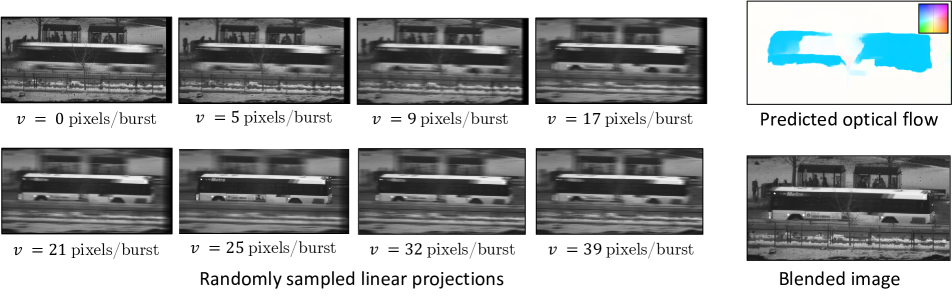
Supplementary Figure 7: An example of motion stack blending. (left) We sample $8$ linear projections randomly along the road’s orientation such that their ensuing pixel displacements are uniformly between $0$ and $40$ pixels. (right) We then blend them using the optical flow field that is predicted between two short exposures computed from the same photon-cube. The flow field visualization follows Baker et al. [2].

4 Experimental Setup for Secs. 6.1 and 6.2

Cameras and Sensory Arrays Used

We used the following imagers for our experiments described in Secs. 6.1 and 6.2:

• SwissSPAD2 array a $512\times 512$ SPAD array that can be operated at a maximum frame rate of $97$ kHz. We operate the SwissSPAD2 in its ‘half-array’ mode: utilizing one of two sub-arrays, with a resolution of $512\times 256$ pixels. The SPAD pixels have a pixel pitch of $16.4$ $\mu$m and a low fill factor of $10$%, owing to the lack of microlenses in the prototype.

• Prophesee EVK4 event camera, which is a state-of-the-camera commercial event camera featuring a sensor resolution of $1280\times 720$ pixels, pixel pitch of $4.86$ $\mu$m and a fill-factor of $>77$%.

• Photron infinicam a conventional high-speed camera that can stream acquisition over USB-C at a resolution of $1246\times 1024$ pixels and $1$ kHz frame-rate. For higher frame rates, it is necessary to reduce the number of rows that are read out—for the example, we use a resolution of $1246\times 240$ pixels to obtain acquisition at $4$ kHz in Fig. 10.

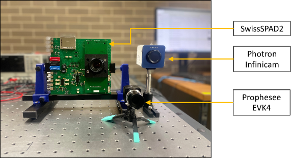
Supplementary Figure 8: Cameras and sensor arrays used for the experiments described in Secs. 6.1 and 6.2. The Infinicam and Prophesee were used for the comparisons made in Figs. 10 and 9 respectively.

Removing Hot Pixels

A few SPAD pixels (around $5$% of the total pixels in our prototype) have extremely high dark current rate and therefore have $B_{t}(\mathbf{x})=1$ almost always. We detect these hot pixels by capturing a photon-cube of $100000$ bit-planes in a very dark environment and detecting pixel locations with high photon counts. For video compressive and event imagers, we inpaint projections using OpenCV’s implementation of the Telea algorithm [18]. For motion projections, we do not sum over bit-plane locations that correspond to hot pixels during integration. Further, we remove pixel locations from the hot pixel mask if the motion trajectory provides access to neighboring values that are not hot pixels. We inpaint the motion projection after excluding these points.

Experiment-wise Lens Specifications

We used C-mount lenses for our experiments with the following focal lengths:

• $12$ mm for the comparison to Prophesee EVK4 in Fig. 9. The Prophesee EVK4 and the SwissSPAD2 were used with the same lens specifications.

• $16$ mm for the coded exposures shown in Fig. 2.

• $35$ mm for the spinning casino roulette shown in Figs. 4 and 10.

• $50$ mm for the motion stack shown in Fig. 6 and the traffic scene shown in Fig. 8.

• $75$ mm for the falling die sequence shown in Fig. 1, the measure tape sequence shown in Fig. 5, and the water splash captured in Fig. 7.

5 UltraPhase Experiments

Processor Description

The chip consists of a $3\times 6$ array of processing cores, each of which can interface with $4\times 4$ SPAD pixels via $3$D stacking. At this point, the $3$D stacking has not been completed, so we interface UltraPhase with the photon-cubes acquired by the SwissSPAD2 [19] instead. Every core is independent, has $4$ kb of available RAM, and can execute programs of up to 256 instructions in length at a rate of $140$ million instructions per second (MIPS). The system supports a wide range of instructions including, bit-wise operations, 32-bit arithmetic operations, data manipulation and custom inter-core synchronization. For more details, please refer to Ardelean [1].

We implement projections on UltraPhase by using a custom assembly code to program each core separately. We include the commented assembly code for all three projections in Figs. 10, 11 and 12. To compute multiple projections, we simply run projections sequentially, one bit-plane at a time. Since each projection can be computed significantly faster than the camera frame rate (e.g., $1.678$ ms for video compressive sensing of $40$ Hz readout), this does not bottleneck acquisition. We include the processing time for each projection in Tab. 1.

Measuring Bandwidth

We assume that the outputs for sum, video compressive and motion projections have $12$-bit depth. For event cameras, we assume that each event consists of $18$-bits—-$9$-bits to encode the pixel location ($\left\lceil\log_{2}(12\times 24)\right\rceil$), $8$ bits to represent the timestamp (corresponding to the bit-plane index where the event was triggered), and $1$-bit to encode polarity. We then measure readout on a $12\times 24$ region-of-interest (RoI) of the falling die sequence that was acquired using the SwissSPAD2. Table 1 lists the readout bandwidth for each projection.

Measuring Power

The power consumption of UltraPhase is comprised of compute power and readout power. For compute power, the chip was characterized by executing instructions corresponding to each projection in an infinite loop and measuring its average power consumption. As an upper bound, we assumed the maximum possible power consumption for operations that involved reading and writing to the RAM. This measured power consumption was then scaled by the duty cycle of each projection—which is the ratio of the time required to process a bit-plane to the exposure time of each bit-plane.

For readout power, we consider a conventional digital interface at $3.3$ V with a load of $7$ pF operating at the specified bandwidth, amounting to $54$ nanowatts for each kilobit readout (nW/kbps)—this is similar, for instance, to the USB interface utilized by the SwissSPAD2.

Table 1 provides the processing power, readout power and the total power for each projection. Clearly, processing requires an order of magnitude (or more) lesser power than readout, which explains how computing photon-cube projections results in reduced sensor power consumption.

Table 1: Power and bandwidth benchmarks when computing photon-cube projections on UltraPhase, a $24\times 12$ array, at $40$ Hz readout. We compare computing projections to reading out the entire photon-cube. We report the processing time, the readout bandwidth, and the compute and readout power for each projection.

	Processing time $\downarrow$	Bandwidth $\downarrow$	Power $\downarrow$
	(ms)	(kbps)	Processing ($\mu$W)	Readout ($\mu$W)	Total ($\mu$W)
12-bit sum image	$0.981$	$135$	$0.3$	$7.29$	$7.6$
Snapshot compressive	$1.678$	$135$	$3.0$	$7.29$	$10.3$
Motion projection	$1.096$	$135$	$1.3$	$7.29$	$8.6$
Event camera	$9.817$	$101.25$	$2.4$	$5.83$	$8.2$
Three projections	$12.591$	$405$	$6.7$	$21.87$	$28.6$
Photon-cube readout	$0.007$	$28125$	$5.4\times 10^{-3}$	$1518.8$	$1518.8$

Comparison to CMOS Sensors

In addition to compute and readout power quantified in the previous section, a computational SPAD also consumes power to detect photons. By incorporating this photon-detection power, we can provide a rough comparison of SoDaCam projections to CMOS sensors. The photon-detection dissipation depends on the number of photon detections, and hence varies with the light level—for the SwissSPAD2, this is measured to be $<1$mW in the dark and $\scriptstyle\sim$$62$ mW in indoor lighting [19]. To estimate compute and readout power, we linearly scale the measurements presented in Tab. 1 for an array of $512\times 256$ pixels. We note that this is a conservative estimate since UltraPhase is not designed to be a low-power device.

As seen in Tab. 1, under ambient lighting, the power consumption of our emulated cameras is higher than conventional CMOS cameras; while in low light, the SPAD consumes lesser power owing to fewer photon detections. We remark that without the bandwidth reduction facilitated by photon-cube projections, SPADs are at a considerable disadvantage compared to their CMOS counterparts. Finally, we provide a comparison against high-speed CMOS cameras, which can also be used to obtain photon-cube projections, albeit with a read noise penalty (Sec. 6.2), and higher power consumption.

Table 2: Power consumption of SoDaCam versus conventional cameras (in mW), estimated for $512\times 256$ pixels at $40$ Hz readout. CMOS estimates assume the usage of column-parallel ADCs [15].

	Photon detection		Compute	Readout	Total
	Dark	Ambient			Dark	Ambient
Photon-cube readout	$1$	$62$	-	$690$	$691$	$752$
Sum-image	$1$	$62$	$0.3$	$4.5$	$5.8$	$66.8$
VCS	$1$	$62$	$1.3$	$4.5$	$6.8$	$67.8$
Motion proj.	$1$	$62$	$0.7$	$4.5$	$6.2$	$67.2$
Event camera	$1$	$62$	$1$	$3.6$	$5.6$	$66.6$
Three proj.(s)	$1$	$62$	$3$	$13.5$	$17.5$	$78.5$
CMOS @ 40 FPS	${\raise 0.73193pt\hbox{$\scriptstyle\sim$}}10$–$25$		-	$4.5$	${\raise 0.73193pt\hbox{$\scriptstyle\sim$}}15$–$30$
CMOS @ 4k FPS	${\raise 0.73193pt\hbox{$\scriptstyle\sim$}}600$–$2500$		-	$450$	${\raise 0.73193pt\hbox{$\scriptstyle\sim$}}1000$–$3000$

Visualization of Projections

Since UltraPhase is a low-resolution sensor-processor ($12\times 24$ pixels), we visualize projections by repeating computations in a tiled manner to cover a region-of-interest (RoI) of $60\times 60$ pixels. Supplementary Figure 9 shows the visualization of an event camera emulated on UltraPhase. To provide more context, we include the CPU visualization of the entire SwissSPAD2 event-frame. We also verified that the outputs of UltraPhase were identical to CPU-run outputs by computing the RMSE between event frames that result from UltraPhase computations and CPU computations (see error map in Supp. Fig. 9).

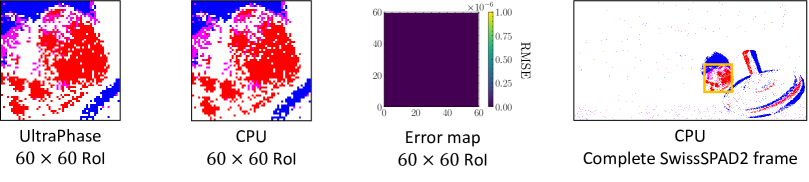
Supplementary Figure 9: Event camera computed using UltraPhase, on $2500$ bit-planes of the falling die sequence. For visualization purposes, we run computations on UltraPhase in a tiled manner so as to cover a RoI of $60\times 60$ pixels. We compare this to CPU-run outputs of the same RoI and verify that they are identical. For context, we highlight this RoI using a bounding box on the CPU-run event-frame that has a resolution of $256\times 512$ pixels. The event simulation parameters used were $\tau=0.45,\beta=0.95,T_{0}=80$.

Custom assembly code for implementing video compressive sensing on UltraPhase. Here, we consider computing one compressive snapshot that is multiplexed by $16$ binary random masks.

⬇

–RAM(64..127) stores the 64 subframe compression code masks as one bit per pixel in byte1 and byte0

–The output is available in RAM(0..15)

–CtrlOut is strobed after every binary frame

\par#define pixelValue 0 –register R0 is used for the pixel values

#define frameIdx 1 –register R1 is used as a counter for the current binary frame

#define subFrameIdx 2 –register R2 is used as a counter for the current subFrame

#define mask 3 –register R3 is used to store the compression codes for the current subframe

#define aux0 4 –register R4 is used for

#define aux1 5 –register R5 is used for

#define CtrlOut 0b10000 –address for external trigger signal

#define toMask 0b001000 –address used to fetch to R3 (mask)

\par0: LOAD subFrameIdx, $64, 0 –initialize subFrame pointer to 0 + 64 (RAM offset)

1: LOAD subFrameIdx, $0, 1

2: LOAD frameIdx, $16, 0 –initialize frameIdx pointer to 16 i.e. number of bit_planes_per_subframe

3: LOAD frameIdx, $0, 1

\par4: GETP 5, 1, 0 –get pixel data and store it in R0 (pixelValue)

5: FETCH @subFrameIdx, toMask, 0 –get the appropriate mask

6: AND pixelValue, mask, pixelValue –apply mask i.e. multiply with code[subframe]

7: CALL 50 –accumulate pixels

8: TELL CtrlOut, 0 –strobe CtrlOut \par—————————————————–

– update indexes

9: OR aux0, aux0, aux0 –clear flags

10: SUBC frameIdx, $1 –decrement frameIdx

11: JUMPZ 13 –check if we finished with all the binary planes per subframe

12: JUMP 4 –if not, then move on

13: OR aux0, aux0, aux0 –clear flags

14: ADDC subFrameIdx, $1 –move to next subFrame

15: JUMP 2 –reset frameIdx and continue

\par—————————————————–

– this subroutine will accumulate the pixel values from pixelValue

50: LOAD aux0, $16, 0 –set R4 (aux0) to 16

51: LOAD aux0, $0, 1

52: LOAD aux1, $0, 0 –set R5 (aux1) to 0

53: LOAD aux1, $0, 1

54: OR aux0, aux0, aux0 –clear flags

55: SR0 pixelValue, pixelValue –extract one pixel

56: ADDC (aux0), aux1, (aux0) –increment if pixel is 1

57: SUBC aux0, $1 –decrement counter

58: JUMPNZ 54 –repeat until done with all 16 pixels

59: RET

Custom assembly code for implementing event cameras on UltraPhase.

⬇

–The core will strobe CtrlOut every time an evet took place and the SoC needs to read RAM(0) to get it

\par#define toaux0 0b000010

#define toaux1 0b000100

#define pixelValue 0 –register R0 is used for the binary pixel values

#define aux0 1 –register R1 is used for misc

#define aux1 2 –register R2 is used for misc

#define Bpointer 3 –register R3 is used as a pointer to the reference_average stored in RAM(17..32)

#define Apointer 4 –register R4 is used as a pointer to the current_average stored in RAM(1..16)

#define pixelIdx 5 –register R5 is used for the current pixel index

#define CtrlOut 0b10000 –address for external trigger signal

#define NOut 0b01000 –address for north trigger signal

#define decayAddress 127 –RAM address 127 stores the exponential_decay

#define decayComplementAddress 126 –RAM address 126 stores the value for 1-exponential_decay

#define intervalAddress 125 –RAM address 125 stores the initial_interval

#define thresholdAddress 124 –RAM address 124 storesthe contrast_threshold

#define frameIdxAddress 123 –RAM address 123 stores the frame_index counter

\par\par0: GETP 5, 1, 0 –get pixel data and store it in R0 (pixelValue)

1: LOAD pixelIdx, $0, 1 –set R5 (pixelIdx) to 16 to use as counter for the pixels

2: LOAD pixelIdx, $16, 0

3: LOAD Apointer, $0, 1 –initialize pointers

4: LOAD Apointer, $1, 0

5: LOAD Bpointer, $0, 1

6: LOAD Bpointer, $17, 0

\par7: FETCH @decayAddress, toaux0, 0 –get decay constant from RAM and store it into R1 (aux0)

8: FETCH @decayComplementAddress, toaux1, 0 –get (1 - decay) constant from RAM and store it into R2 (aux1)

\par9: MUL (Apointer), aux0, (Apointer) – current_average[pixelIdx] = exponential_decay * current_average[pixelIdx]

10: SRX (Apointer), (Apointer) – 8 fractional bit multiplication

11: SRX (Apointer), (Apointer)

12: SRX (Apointer), (Apointer)

13: SRX (Apointer), (Apointer)

14: SRX (Apointer), (Apointer)

15: SRX (Apointer), (Apointer)

16: SRX (Apointer), (Apointer)

17: SRX (Apointer), (Apointer)

\par18: SR0 pixelValue, pixelValue –shift R0 (pixelValue) to the right and pad with 0; the pixel bit is loaded into the carry flag

19: JUMPNC 21 –current_average[pixelIdx] = current_average[pixelIdx] + (1-exponential_decay) * 0

20: ADD (Apointer), aux1, (Apointer) –current_average[pixelIdx] = current_average[pixelIdx] + (1-exponential_decay) * 1

21: FETCH @frameIdxAddress, toaux0, 0 –get frame_index from RAM and store it into R1 (aux0)

22: FETCH @intervalAddress, toaux1, 0 –get initial_interval from RAM and store it into R2 (aux1)

23: CMP aux0, aux1 –check if frame_index < initial_interval

24: JUMPNC 40 –if not, jump and process

25: FETCH (Apointer), toaux0, 0 –if yes, get current_average[pixelIdx]

26: STORE aux0, (Bpointer) –reference_average[pixelIdx] = current_average[pixelIdx]

27: JUMP 70 –GO TO NEXT PIXEL

\par– frame_index is larger than initial_interval

40: FETCH (Apointer), toaux0, 0 –if not, get current_average[pixelIdx] and store it into R1 (aux0)

41: FETCH (Bpointer), toaux1, 0 –get reference_average[pixelIdx] and store it into R2 (aux1)

42: SUB aux0, aux1, aux0 –diff[pixelIdx] = current_average[pixelIdx] - reference_average[pixelIdx] and store it into R1 (aux0)

43: JUMPNC 60 –diff is positive

\par– compare abs(diff) with threshold if diff is negative

44: FETCH @thresholdAddress, toaux1, 0 –get contrast_threshold and store it into R2 (aux1)

45: NEG aux1, aux1 –diff is negative, so make contrast_threshold negative and store it into R2 (aux1)

46: CMP aux0, aux1 –if diff < -contrast_threshold

47: JUMPNC 70 –if not, GO TO NEXT PIXEL

48: NEG pixelIdx, @0 –RAM(0) = -pixel_index i.e. a negative event

49: ADD (Bpointer), aux1, (Bpointer) –reference_average += contrast_threshold * (-1)

50: TELL CtrlOut, 0 –strobe CtrlOut to signal an event

51: JUMP 70 –GO TO NEXT PIXEL

\par– compare abs(diff) with threshold if diff is positive

60: FETCH @thresholdAddress, toaux1, 0 –get contrast_threshold and store it into R2 (aux1)

61: CMP aux1, aux0 –if diff > contrast_threshold

62: JUMPNC 70 –if not, GO TO NEXT PIXEL

63: STORE pixelIdx, @0 –RAM(0) = pixel_index i.e. a positive event

64: ADD (Bpointer), aux1, (Bpointer) –reference_average += contrast_threshold * 1

65: TELL CtrlOut, 0 –strobe CtrlOut to signal an event

66: JUMP 70 –GO TO NEXT PIXEL

\par–GO TO NEXT PIXEL

70: OR pixelValue, pixelValue, pixelValue –clear flags

71: ADDC Apointer, $1 –increment Apointer

72: ADDC Bpointer, $1 –increment Bpointer

73: SUBC pixelIdx, $1 –decrement pixel counter

74: JUMPNZ 7 –if not done with pixels, go to next one

75: FETCH @frameIdxAddress, toaux0, 0 –if done with pixels, increment frame counter and get new pixel values

76: TELL NOut, 0 –strobe NOut to signal a new exposure

77: ADDC aux0, $1

78: STORE aux0, @frameIdxAddress

79: JUMP 0

Custom assembly code for implementing motion projections on UltraPhase. Without loss of generality, we consider a linear projection along the horizontal direction.

⬇

–The projection is available in RAM(0..15)

– CtrlOut is strobed after every frame

\par#define Xshift 0 –register R0 is used for the horizontal shift

#define timestep 1 –register R1 is used for the current timestep

#define origPixels 2 –register R2 is used for the current core’s pixels

#define shiftPixels 3 –register R3 is used for the shifted pixels

#define aux0 4 –register R4 is used for misc

#define aux1 5 –register R5 is used for misc

#define CtrlOut 0b10000 –address for external trigger signal

#define shiftL3neighAddr 127 –RAM(127) stores the 0b0111_0111_0111_0111 mask

#define shiftL3currAddr 126 –RAM(126) stores the 0b1000_1000_1000_1000 mask

#define shiftL2neighAddr 125 –RAM(125) stores the 0b0011_0011_0011_0011 mask

#define shiftL2currAddr 124 –RAM(124) stores the 0b1100_1100_1100_1100 mask

#define shiftL1neighAddr 123 –RAM(123) stores the 0b0001_0001_0001_0001 mask

#define shiftL1currAddr 122 –RAM(122) stores the 0b1110_1110_1110_1110 mask

\par0: LOAD Xshift, $0xFFF8, 0 –load -8 into Xshift as initial value

1: LOAD Xshift, $0xFFFF, 1

2: CALL 50 –get the correct pixel values according to Xshift

3: CALL 30 –accumulate pixels

4: CALL 20 –advance time

5: TELL CtrlOut, 0 – strobe CtrlOut to signal a new frame

6: JUMP 2 –repeat

\par—————————————————–

– this subroutine will advance timestep and update Xshift

20: OR timestep, timestep, timestep –clear flags

21: ADDC timestep, $1 –increment timestep

22: OR timestep, timestep, aux0 –copy timestep to aux0

23: SPLIT aux0, 5, 0b010000 –timestep = timestep/1024

24: SR0 aux0, aux0 25: SR0 aux0, aux0 26: LOAD aux1, $1, 0 –load aux1 with the Xspeed value of 1

27: MAC aux0, aux1, Xshift, Xshift –Xshift += Xspeed*timestep/2

28: RET

\par—————————————————–

– this subroutine will accumulate the pixel values from shiftPixels

30: LOAD aux0, $16, 0 –set R4 (aux0) to 16

31: LOAD aux0, $0, 1

32: LOAD aux1, $0, 0 –set R5 (aux1) to 0

33: LOAD aux1, $0, 1

34: OR aux0, aux0, aux0 –clear flags

35: SR0 shiftPixels, shiftPixels –extract one pixel

36: ADDC (aux0), aux1, (aux0) –increment if pixel is 1

37: SUBC aux0, $1 –decrement counter

38: JUMPNZ 34 –repeat until done with all 16 pixels

39: RET

\par—————————————————–

– this subroutine will get pixel values from the core and the correct neighbour based on the Xshift

50: GETP 5, 4, 0 –get pixel values and store them in R2 (origPixels)

51: OR Xshift, Xshift, aux1 –copy current shift into R5 (aux1)

52: LOAD aux0, $0, 0 –set R4 (aux0) to 0 to use for Xshift comparison

53: LOAD aux0, $0, 1

54: CMP aux1, aux0 –compare current shift with 0

55: JUMPZ 115 –current shift = 0

56: JUMPC 120 –current shift < 0

57: JUMP 58 –current shift > 0

——————————-

– positive shifts

58: LOAD aux0, $4, 0 –set R4 (aux0) to 4 for current shift comparison

59: LOAD aux0, $0, 1

60: CMP aux0, aux1

61: JUMPC 105 –current shift > 4, read from the neighbour’s neighbour

62: JUMPZ 100 –current shift is 4

63: LOAD aux0, $2, 0 –set R4 (aux0) to 2, for current shift comparison

64: CMP aux0, aux1

65: JUMPC 90 –current shift is 3

66: JUMPZ 80 –current shift is 2

\par– shift is 1

67: SL0 shiftPixels, shiftPixels –pixels from the neighbour need to be shifted to the left 3 times

68: SL0 shiftPixels, shiftPixels

69: SL0 shiftPixels, shiftPixels

70: OR origPixels, origPixels, aux1 –save curent pixels in the aux1 variable

71: SR0 aux1, aux1 –pixels from this core need to be shifted to the right once

72: AND shiftPixels, @shiftL3currAddr, shiftPixels –apply mask to select relevant bits from neighbour

73: AND aux1, @shiftL3neighAddr, aux1 –apply mask to select relevant bits from current core

74: OR shiftPixels, aux1, shiftPixels –combine to create final pixel values

75: RET

\par– shift is 2

80: SL0 shiftPixels, shiftPixels –pixels from neighbour need to be shifted to the left 2 times

81: SL0 shiftPixels, shiftPixels

82: OR origPixels, origPixels, aux1 –save curent pixels in the aux1 variable

83: SR0 aux1, aux1 –pixels from this core need to be shifted to the right 2 times

84: SR0 aux1, aux1

85: AND shiftPixels, @shiftL2currAddr, shiftPixels –apply mask to select relevant bits from neighbour

86: AND aux1, @shiftL2neighAddr, aux1 –apply mask to select relevant bits from current core

87: OR shiftPixels, aux1, shiftPixels –combine to create final pixel values

88: RET

\par– shift is 3

90: SL0 shiftPixels, shiftPixels –pixels from neighbour need to be shifted to the left once

91: OR origPixels, origPixels, aux1 –save curent pixels in the aux1 variable

92: SR0 aux1, aux1 –pixels from this core need to be shifted to the right 3 times

93: SR0 aux1, aux1

94: SR0 aux1, aux1

95: AND shiftPixels, @shiftL1currAddr, shiftPixels –apply mask to select relevant bits from neighbour

96: AND aux1, @shiftL1neighAddr, aux1 –apply mask to select relevant bits from current core

97: OR shiftPixels, aux1, shiftPixels –combine to create final pixel values

98: RET

\par– shift is 4

100: PUTN origPixels, 4 –shift your pixels to the left (share pixels with neighbour)

101: SAVEN 1 –save pixels from rigth neighbour

102: GETN 0, 8, 0 –get pixels from rigth neighbour and store in shiftPixels

103: RET

\par– shift is > 4

105: PUTN origPixels, 4 –shift your pixels to the left (share pixels with neighbour)

106: SAVEN 1 –save pixels from right neighbour

107: GETN 0, 8, 0 –get pixels from right neighbour and store in shiftPixels

108: OR aux1, aux1, aux1 –clear Carry flag

109: SUBC aux1, $4 –subtract 4 from current shift because we read from a neighbour

110: JUMP 58

\par——————————-

– shift is zero

115: OR origPixels, origPixels, shiftPixels –the shift is zero, so keep the pixels

116: RET

\par——————————-

– negative shifts

120: LOAD aux0, $FFFC, 0 –set R4 (aux0) to -4 to use for current shift comparison

121: LOAD aux0, $0xFFFF, 1

122: CMP aux1, aux0

123: JUMPC 170 –current shift < -4 so we need to read from neighbour’s neighbour

124: JUMPZ 160 –current shift is -4

125: LOAD aux0, $FFFE, 0 –set R4 (aux0) to -2 to use for current shift comparison

126: CMP aux1, aux0

127: JUMPC 150 –current shift is -3

128: JUMPZ 140 –current shift is -2

\par– shift is -1

129: SR0 shiftPixels, shiftPixels –pixels from neighbour need to be shifted to the right 3 times

130: SR0 shiftPixels, shiftPixels

131: SR0 shiftPixels, shiftPixels

132: OR origPixels, origPixels, aux1 –save curent pixels in the aux1 variable

133: SL0 aux1, aux1 –pixels from this core need to be shifted to the left once

134: AND shiftPixels, @shiftL1neighAddr, shiftPixels –apply mask to select relevant bits from neighbour

135: AND aux1, @shiftL1currAddr, aux1 –apply mask to select relevant bits from current core

136: OR shiftPixels, aux1, shiftPixels –combine to create final pixel values

137: RET

\par– shift is -2

140: SR0 shiftPixels, shiftPixels –pixels from neighbour need to be shifted to the right 2 times

141: SR0 shiftPixels, shiftPixels

142: OR origPixels, origPixels, aux1 –save curent pixels in the aux1 variable

143: SL0 aux1, aux1 –pixels from this core need to be shifted to the left 2 times

144: SL0 aux1, aux1

145: AND shiftPixels, @shiftL2neighAddr, shiftPixels –apply mask to select relevant bits from neighbour

146: AND aux1, @shiftL2currAddr, aux1 –apply mask to select relevant bits from current core

147: OR shiftPixels, aux1, shiftPixels –combine to create final pixel values

148: RET

\par– shift is -3

150: SR0 shiftPixels, shiftPixels –pixels from neighbour need to be shifted to the right once

151: OR origPixels, origPixels, aux1 –save curent pixels in the aux1 variable

152: SL0 aux1, aux1 –pixels from this core need to be shifted to the left 3 times

153: SL0 aux1, aux1

154: SL0 aux1, aux1

155: AND shiftPixels, @shiftL3neighAddr, shiftPixels –apply mask to select relevant bits from neighbour

156: AND aux1, @shiftL3currAddr, aux1 –apply mask to select relevant bits from current core

157: OR shiftPixels, aux1, shiftPixels –combine to create final pixel values

158: RET

\par– shift is -4

160: PUTN origPixels, 1 –shift your pixels to the right (share pixels with neighbour)

161: SAVEN 4 –save pixels from left neighbour

162: GETN 2, 8, 0 –get pixels from left neighbour and store in shiftPixels

163: RET

\par– shift is < -4

170: PUTN origPixels, 1 –shift your pixels to the right (share pixels with neighbour)

171: SAVEN 4 –save pixels from left neighbour

172: GETN 2, 8, 0 –get pixels from left neighbour and store in shiftPixels

173: OR aux1, aux1, aux1 –clear Carry flag

174: ADDC aux1, $4 –add 4 to current shift because we read from a neighbour

175: JUMP 120

References

- [1] Phantom-v2640. https://www.phantomhighspeed.com/products/cameras/ultrahigh4mpx/v2640. Accessed: 2023-01-28.
- Adelson et al. [1991] E. H. Adelson, J. R. Bergen, et al. The plenoptic function and the elements of early vision. Computational models of visual processing, 1(2):3–20, 1991.
- Agrawal et al. [2010] A. Agrawal, A. Veeraraghavan, and R. Raskar. Reinterpretable imager: Towards variable post-capture space, angle and time resolution in photography. In Computer Graphics Forum, volume 29, pages 763–772. Wiley Online Library, 2010.
- Antolovic et al. [2016] I. M. Antolovic, S. Burri, C. Bruschini, R. Hoebe, and E. Charbon. Nonuniformity analysis of a 65-kpixel CMOS SPAD imager. IEEE Transactions on Electron Devices, 63(1):57–64, 2016. doi: 10.1109/TED.2015.2458295.
- Ardelean [2023] A. Ardelean. Computational Imaging SPAD Cameras. PhD thesis, École polytechnique fédérale de Lausanne, 2023.
- Boukhayma et al. [2016] A. Boukhayma, A. Peizerat, and C. Enz. A sub-0.5 electron read noise VGA image sensor in a standard CMOS process. IEEE Journal of Solid-State Circuits, 2016.
- Canny [1986] J. Canny. A computational approach to edge detection. IEEE Transactions on Pattern Analysis and Machine Intelligence, PAMI-8(6):679–698, 1986. doi: 10.1109/TPAMI.1986.4767851.
- Carey et al. [2013] S. J. Carey, A. Lopich, D. R. Barr, B. Wang, and P. Dudek. A 100,000 fps vision sensor with embedded 535GOPS/W 256×256 SIMD processor array. In 2013 Symposium on VLSI Circuits, pages C182–C183, 2013.
- Chen et al. [2017] J. Chen, S. J. Carey, and P. Dudek. Feature extraction using a portable vision system. In IEEE/RSJ Int. Conf. Intell. Robots Syst., Workshop Vis.-based Agile Auton. Navigation UAVs, volume 2, 2017.
- Chen and Guo [2019] S. Chen and M. Guo. Live demonstration: Celex-v: A 1m pixel multi-mode event-based sensor. In Proceedings of the IEEE/CVF Conference on Computer Vision and Pattern Recognition (CVPR) Workshops, June 2019.
- Dalal and Triggs [2005] N. Dalal and B. Triggs. Histograms of oriented gradients for human detection. In 2005 IEEE computer society conference on computer vision and pattern recognition (CVPR’05), volume 1, pages 886–893. Ieee, 2005.
- Debevec and Malik [1997] P. E. Debevec and J. Malik. Recovering high dynamic range radiance maps from photographs. In Proceedings of the 24th Annual Conference on Computer Graphics and Interactive Techniques, page 369–378. ACM Press/Addison-Wesley Publishing Co., 1997. doi: 10.1145/258734.258884. URL https://doi.org/10.1145/258734.258884.
- Della Rocca et al. [2020] F. M. Della Rocca, H. Mai, S. W. Hutchings, T. Al Abbas, K. Buckbee, A. Tsiamis, P. Lomax, I. Gyongy, N. A. Dutton, and R. K. Henderson. A 128 128 SPAD motion-triggered time-of-flight image sensor with in-pixel histogram and column-parallel vision processor. IEEE Journal of Solid-State Circuits, 55(7):1762–1775, 2020.
- Finateu et al. [2020] T. Finateu, A. Niwa, D. Matolin, K. Tsuchimoto, A. Mascheroni, E. Reynaud, P. Mostafalu, F. Brady, L. Chotard, F. LeGoff, H. Takahashi, H. Wakabayashi, Y. Oike, and C. Posch. 5.10 a 1280×720 back-illuminated stacked temporal contrast event-based vision sensor with 4.86µm pixels, 1.066GEPS readout, programmable event-rate controller and compressive data-formatting pipeline. In 2020 IEEE International Solid- State Circuits Conference - (ISSCC), pages 112–114, 2020. doi: 10.1109/ISSCC19947.2020.9063149.
- Fossum [2005] E. R. Fossum. What to do with sub-diffraction-limit (SDL) pixels?—a proposal for a gigapixel digital film sensor (DFS). In IEEE Workshop on Charge-Coupled Devices and Advanced Image Sensors, pages 214–217, 2005.
- Fossum [2011] E. R. Fossum. The quanta image sensor (QIS): Concepts and challenges. In Imaging and Applied Optics, page JTuE1. Optica Publishing Group, 2011. doi: 10.1364/COSI.2011.JTuE1. URL http://opg.optica.org/abstract.cfm?URI=COSI-2011-JTuE1.
- Fossum et al. [2016] E. R. Fossum, J. Ma, S. Masoodian, L. Anzagira, and R. Zizza. The quanta image sensor: Every photon counts. Sensors, 16(8):1260, 2016.
- Gehrig et al. [2020] D. Gehrig, H. Rebecq, G. Gallego, and D. Scaramuzza. Eklt: Asynchronous photometric feature tracking using events and frames. International Journal of Computer Vision, 128(3):601–618, 2020.
- Graca and Delbruck [2021] R. Graca and T. Delbruck. Unraveling the paradox of intensity-dependent DVS pixel noise. arXiv preprint arXiv:2109.08640, 2021.
- Gupta et al. [2010] M. Gupta, A. Agrawal, A. Veeraraghavan, and S. G. Narasimhan. Flexible voxels for motion-aware videography. In Computer Vision–ECCV 2010: 11th European Conference on Computer Vision, Heraklion, Crete, Greece, September 5-11, 2010, Proceedings, Part I 11, pages 100–114. Springer, 2010.
- Gutierrez-Barragan et al. [2022] F. Gutierrez-Barragan, A. Ingle, T. Seets, M. Gupta, and A. Velten. Compressive single-photon 3D cameras. In Proceedings of the IEEE/CVF Conference on Computer Vision and Pattern Recognition (CVPR), pages 17854–17864, June 2022.
- Gyongy et al. [2018] I. Gyongy, N. A. Dutton, and R. K. Henderson. Single-photon tracking for high-speed vision. Sensors, 18(2):323, 2018.
- Gyongy et al. [2020] I. Gyongy, S. W. Hutchings, A. Halimi, M. Tyler, S. Chan, F. Zhu, S. McLaughlin, R. K. Henderson, and J. Leach. High-speed 3D sensing via hybrid-mode imaging and guided upsampling. Optica, 7(10):1253–1260, 2020.
- Harris et al. [1988] C. Harris, M. Stephens, et al. A combined corner and edge detector. In Alvey vision conference, volume 15, pages 10–5244. Citeseer, 1988.
- Hidalgo-Carrió et al. [2022] J. Hidalgo-Carrió, G. Gallego, and D. Scaramuzza. Event-aided direct sparse odometry. In Proceedings of the IEEE/CVF Conference on Computer Vision and Pattern Recognition (CVPR), pages 5781–5790, June 2022.
- Horn and Schunck [1981] B. K. Horn and B. G. Schunck. Determining optical flow. Artificial intelligence, 17(1-3):185–203, 1981.
- Hu et al. [2021] Y. Hu, S.-C. Liu, and T. Delbruck. v2e: From video frames to realistic DVS events. In Proceedings of the IEEE/CVF Conference on Computer Vision and Pattern Recognition (CVPR) Workshops, pages 1312–1321, June 2021.
- Igual [2019] J. Igual. Photographic noise performance measures based on raw files analysis of consumer cameras. Electronics, 8(11):1284, 2019.
- Ingle et al. [2019] A. Ingle, A. Velten, and M. Gupta. High Flux Passive Imaging With Single-Photon Sensors. In Proceedings of the IEEE/CVF Conference on Computer Vision and Pattern Recognition (CVPR), June 2019.
- Ingle et al. [2021] A. Ingle, T. Seets, M. Buttafava, S. Gupta, A. Tosi, M. Gupta, and A. Velten. Passive inter-photon imaging. In Proceedings of the IEEE/CVF Conference on Computer Vision and Pattern Recognition (CVPR), June 2021.
- Iwabuchi et al. [2021] K. Iwabuchi, Y. Kameda, and T. Hamamoto. Image quality improvements based on motion-based deblurring for single-photon imaging. IEEE Access, 9:30080–30094, 2021. doi: 10.1109/ACCESS.2021.3059293.
- Jiang et al. [2021] Y. Jiang, I. Choi, J. Jiang, and J. Gu. HDR video reconstruction with tri-exposure quad-bayer sensors. arXiv preprint arXiv:2103.10982, 2021.
- Levin et al. [2008] A. Levin, P. Sand, T. S. Cho, F. Durand, and W. T. Freeman. Motion-invariant photography. ACM Transactions on Graphics (TOG), 27(3):1–9, 2008.
- Levoy and Hanrahan [1996] M. Levoy and P. Hanrahan. Light field rendering. In Proceedings of the 23rd annual conference on Computer graphics and interactive techniques, pages 31–42, 1996.
- Li et al. [2020] Y. Li, M. Qi, R. Gulve, M. Wei, R. Genov, K. N. Kutulakos, and W. Heidrich. End-to-end video compressive sensing using anderson-accelerated unrolled networks. In 2020 IEEE International Conference on Computational Photography (ICCP), pages 1–12, 2020. doi: 10.1109/ICCP48838.2020.9105237.
- Lichtsteiner [2003] P. Lichtsteiner. 64x64 event-driven logarithmic temporal derivative silicon retina. In Program 2003 IEEE Workshop on CCD and AIS, 2003.
- Liu et al. [2022] Y. Liu, F. Gutierrez-Barragan, A. Ingle, M. Gupta, and A. Velten. Single-photon camera guided extreme dynamic range imaging. In Proceedings of the IEEE/CVF Winter Conference on Applications of Computer Vision (WACV), pages 1575–1585, January 2022.
- Llull et al. [2013] P. Llull, X. Liao, X. Yuan, J. Yang, D. Kittle, L. Carin, G. Sapiro, and D. J. Brady. Coded aperture compressive temporal imaging. Opt. Express, 21(9):10526–10545, May 2013. doi: 10.1364/OE.21.010526. URL https://opg.optica.org/oe/abstract.cfm?URI=oe-21-9-10526.
- Lucas and Kanade [1981] B. D. Lucas and T. Kanade. An iterative image registration technique with an application to stereo vision. In IJCAI’81: 7th international joint conference on Artificial intelligence, volume 2, pages 674–679, 1981.
- Ma et al. [2017] J. Ma, S. Masoodian, D. A. Starkey, and E. R. Fossum. Photon-number-resolving megapixel image sensor at room temperature without avalanche gain. Optica, 4(12):1474–1481, Dec 2017. doi: 10.1364/OPTICA.4.001474. URL http://www.osapublishing.org/optica/abstract.cfm?URI=optica-4-12-1474.
- Ma et al. [2020] S. Ma, S. Gupta, A. C. Ulku, C. Bruschini, E. Charbon, and M. Gupta. Quanta burst photography. ACM Transactions on Graphics, 39(4):1–16, July 2020. ISSN 0730-0301, 1557-7368.
- Ma et al. [2023] S. Ma, P. Mos, E. Charbon, and M. Gupta. Burst vision using single-photon cameras. In Proceedings of the IEEE/CVF Winter Conference on Applications of Computer Vision (WACV), pages 5375–5385, January 2023.
- Mann and Picard [1994] S. Mann and R. Picard. Beingundigital’with digital cameras. MIT Media Lab Perceptual, 1:2, 1994.
- Martel et al. [2020] J. N. Martel, L. K. Mueller, S. J. Carey, P. Dudek, and G. Wetzstein. Neural sensors: Learning pixel exposures for HDR imaging and video compressive sensing with programmable sensors. IEEE Transactions on Pattern Analysis and Machine Intelligence, 42(7):1642–1653, 2020.
- Martel et al. [2016] J. N. P. Martel, L. K. Müller, S. J. Carey, and P. Dudek. Parallel HDR tone mapping and auto-focus on a cellular processor array vision chip. In 2016 IEEE International Symposium on Circuits and Systems (ISCAS), pages 1430–1433, 2016. doi: 10.1109/ISCAS.2016.7527519.
- Martel et al. [2017] J. N. P. Martel, L. K. Müller, S. J. Carey, and P. Dudek. High-speed depth from focus on a programmable vision chip using a focus tunable lens. In 2017 IEEE International Symposium on Circuits and Systems (ISCAS), pages 1–4, 2017. doi: 10.1109/ISCAS.2017.8050548.
- Metzler et al. [2020] C. A. Metzler, H. Ikoma, Y. Peng, and G. Wetzstein. Deep optics for single-shot high-dynamic-range imaging. In Proceedings of the IEEE/CVF Conference on Computer Vision and Pattern Recognition (CVPR), June 2020.
- Morimoto et al. [2020] K. Morimoto, A. Ardelean, M.-L. Wu, A. C. Ulku, I. M. Antolovic, C. Bruschini, and E. Charbon. Megapixel time-gated SPAD image sensor for 2D and 3D imaging applications. Optica, 7(4):346–354, Apr. 2020.
- Morimoto et al. [2021] K. Morimoto, J. Iwata, M. Shinohara, H. Sekine, A. Abdelghafar, H. Tsuchiya, Y. Kuroda, K. Tojima, W. Endo, Y. Maehashi, Y. Ota, T. Sasago, S. Maekawa, S. Hikosaka, T. Kanou, A. Kato, T. Tezuka, S. Yoshizaki, T. Ogawa, K. Uehira, A. Ehara, F. Inui, Y. Matsuno, K. Sakurai, and T. Ichikawa. 3.2 megapixel 3D-stacked charge focusing SPAD for low-light imaging and depth sensing. In 2021 IEEE International Electron Devices Meeting (IEDM), pages 20.2.1–20.2.4, 2021. doi: 10.1109/IEDM19574.2021.9720605.
- Namiki et al. [2022] S. Namiki, S. Sato, Y. Kameda, and T. Hamamoto. Imaging method using multi-threshold pattern for photon detection of quanta image sensor. In International Workshop on Advanced Imaging Technology (IWAIT) 2022, volume 12177, page 1217702. SPIE, 2022.
- Nayar et al. [2006] S. K. Nayar, V. Branzoi, and T. E. Boult. Programmable imaging: Towards a flexible camera. International Journal of Computer Vision, 70:7–22, 2006.
- Posch et al. [2011] C. Posch, D. Matolin, and R. Wohlgenannt. A QVGA 143 dB Dynamic Range Frame-Free PWM Image Sensor With Lossless Pixel-Level Video Compression and Time-Domain CDS. IEEE Journal of Solid-State Circuits, 46(1):259–275, 2011. doi: 10.1109/JSSC.2010.2085952.
- Raskar et al. [2006] R. Raskar, A. Agrawal, and J. Tumblin. Coded exposure photography: motion deblurring using fluttered shutter. In Acm Siggraph 2006 Papers, pages 795–804. 2006.
- Rebecq et al. [2019] H. Rebecq, R. Ranftl, V. Koltun, and D. Scaramuzza. Events-to-video: Bringing modern computer vision to event cameras. In Proceedings of the IEEE/CVF Conference on Computer Vision and Pattern Recognition (CVPR), June 2019.
- Reddy et al. [2011] D. Reddy, A. Veeraraghavan, and R. Chellappa. P2C2: Programmable pixel compressive camera for high speed imaging. In CVPR 2011, pages 329–336, 2011. doi: 10.1109/CVPR.2011.5995542.
- Ren et al. [2018] X. Ren, P. W. Connolly, A. Halimi, Y. Altmann, S. McLaughlin, I. Gyongy, R. K. Henderson, and G. S. Buller. High-resolution depth profiling using a range-gated CMOS SPAD quanta image sensor. Optics express, 26(5):5541–5557, 2018.
- Scheerlinck et al. [2020] C. Scheerlinck, H. Rebecq, D. Gehrig, N. Barnes, R. Mahony, and D. Scaramuzza. Fast image reconstruction with an event camera. In Proceedings of the IEEE/CVF Winter Conference on Applications of Computer Vision (WACV), March 2020.
- Seets et al. [2021] T. Seets, A. Ingle, M. Laurenzis, and A. Velten. Motion adaptive deblurring with single-photon cameras. In Proceedings of the IEEE/CVF Winter Conference on Applications of Computer Vision (WACV), pages 1945–1954, January 2021.
- Seo et al. [2017] M.-W. Seo, Y. Shirakawa, Y. Masuda, Y. Kawata, K. Kagawa, K. Yasutomi, and S. Kawahito. 4.3 a programmable sub-nanosecond time-gated 4-tap lock-in pixel cmos image sensor for real-time fluorescence lifetime imaging microscopy. In 2017 IEEE International Solid-State Circuits Conference (ISSCC), pages 70–71, 2017. doi: 10.1109/ISSCC.2017.7870265.
- Serrano-Gotarredona and Linares-Barranco [2013] T. Serrano-Gotarredona and B. Linares-Barranco. A 128 128 1.5% contrast sensitivity 0.9% FPN 3 s latency 4 mW asynchronous frame-free dynamic vision sensor using transimpedance preamplifiers. IEEE Journal of Solid-State Circuits, 48(3):827–838, 2013.
- Shedligeri et al. [2021] P. Shedligeri, A. S, and K. Mitra. A unified framework for compressive video recovery from coded exposure techniques. In Proceedings of the IEEE/CVF Winter Conference on Applications of Computer Vision (WACV), pages 1600–1609, January 2021.
- Shi et al. [2022] C. Shi, N. Song, W. Li, Y. Li, B. Wei, H. Liu, and J. Jin. A review of event-based indoor positioning and navigation. 2022.
- Sitzmann et al. [2018] V. Sitzmann, S. Diamond, Y. Peng, X. Dun, S. Boyd, W. Heidrich, F. Heide, and G. Wetzstein. End-to-end optimization of optics and image processing for achromatic extended depth of field and super-resolution imaging. ACM Transactions on Graphics (TOG), 37(4):114, 2018.
- Taverni et al. [2018] G. Taverni, D. Paul Moeys, C. Li, C. Cavaco, V. Motsnyi, D. San Segundo Bello, and T. Delbruck. Front and back illuminated dynamic and active pixel vision sensors comparison. IEEE Transactions on Circuits and Systems II: Express Briefs, 65(5):677–681, 2018. doi: 10.1109/TCSII.2018.2824899.
- Teed and Deng [2020] Z. Teed and J. Deng. Raft: Recurrent all-pairs field transforms for optical flow. In European Conference on Computer Vision, 2020.
- Tulyakov et al. [2021] S. Tulyakov, D. Gehrig, S. Georgoulis, J. Erbach, M. Gehrig, Y. Li, and D. Scaramuzza. Time lens: Event-based video frame interpolation. In Proceedings of the IEEE/CVF Conference on Computer Vision and Pattern Recognition (CVPR), pages 16155–16164, June 2021.
- Ulku et al. [2019] A. C. Ulku, C. Bruschini, I. M. Antolovic, Y. Kuo, R. Ankri, S. Weiss, X. Michalet, and E. Charbon. A 512 × 512 SPAD Image Sensor With Integrated Gating for Widefield FLIM. IEEE Journal of Selected Topics in Quantum Electronics, 25(1):1–12, Jan. 2019. ISSN 1077-260X, 1558-4542. doi: 10.1109/JSTQE.2018.2867439.
- Wan et al. [2012] G. Wan, X. Li, G. Agranov, M. Levoy, and M. Horowitz. CMOS image sensors with multi-bucket pixels for computational photography. IEEE Journal of Solid-State Circuits, 47(4):1031–1042, 2012. doi: 10.1109/JSSC.2012.2185189.
- Wei et al. [2018] M. Wei, N. Sarhangnejad, Z. Xia, N. Gusev, N. Katic, R. Genov, and K. N. Kutulakos. Coded two-bucket cameras for computer vision. In Proceedings of the European Conference on Computer Vision (ECCV), September 2018.
- White et al. [2022] M. White, S. Ghajari, T. Zhang, A. Dave, A. Veeraraghavan, and A. Molnar. A differential SPAD array architecture in 0.18 m CMOS for HDR imaging. In 2022 IEEE International Symposium on Circuits and Systems (ISCAS), pages 292–296, 2022. doi: 10.1109/ISCAS48785.2022.9937558.
- Yamazaki et al. [2017] T. Yamazaki, H. Katayama, S. Uehara, A. Nose, M. Kobayashi, S. Shida, M. Odahara, K. Takamiya, Y. Hisamatsu, S. Matsumoto, L. Miyashita, Y. Watanabe, T. Izawa, Y. Muramatsu, and M. Ishikawa. 4.9 a 1ms high-speed vision chip with 3D-stacked 140GOPS column-parallel PEs for spatio-temporal image processing. In 2017 IEEE International Solid-State Circuits Conference (ISSCC), pages 82–83, 2017. doi: 10.1109/ISSCC.2017.7870271.
- Yang et al. [2012] F. Yang, Y. M. Lu, L. Sbaiz, and M. Vetterli. Bits from photons: Oversampled image acquisition using binary poisson statistics. IEEE Transactions on Image Processing, 21(4):1421–1436, 2012. doi: 10.1109/TIP.2011.2179306.
- Yuan et al. [2022] X. Yuan, Y. Liu, J. Suo, F. Durand, and Q. Dai. Plug-and-play algorithms for video snapshot compressive imaging. IEEE Transactions on Pattern Analysis and Machine Intelligence, 44(10):7093–7111, 2022. doi: 10.1109/TPAMI.2021.3099035.
- Zhang et al. [2021] J. Zhang, X. Yang, Y. Fu, X. Wei, B. Yin, and B. Dong. Object tracking by jointly exploiting frame and event domain. In Proceedings of the IEEE/CVF International Conference on Computer Vision (ICCV), pages 13043–13052, 2021.
- Zhang et al. [2020] K. Zhang, Y. Li, W. Zuo, L. Zhang, L. Van Gool, and R. Timofte. Plug-and-play image restoration with deep denoiser prior. arXiv preprint, 2020.
- Zhang et al. [2018] R. Zhang, P. Isola, A. A. Efros, E. Shechtman, and O. Wang. The unreasonable effectiveness of deep features as a perceptual metric. In Proceedings of the IEEE Conference on Computer Vision and Pattern Recognition (CVPR), June 2018.
- Zhang et al. [2022] T. Zhang, M. J. White, A. Dave, S. Ghajari, A. Raghuram, A. C. Molnar, and A. Veeraraghavan. First arrival differential LiDAR. In 2022 IEEE International Conference on Computational Photography (ICCP), pages 1–12, 2022. doi: 10.1109/ICCP54855.2022.9887683.
- Zhang and Lin [2017] W. Zhang and L. Lin. Light field flow estimation based on occlusion detection. Journal of Computer and Communications, 5(3):1–9, 2017.