Continual Learning From a Stream of APIs

Abstract

Continual learning (CL) aims to learn new tasks without forgetting previous tasks. However, existing CL methods require a large amount of raw data, which is often unavailable due to copyright considerations and privacy risks. Instead, stakeholders usually release pre-trained machine learning models as a service (MLaaS), which users can access via APIs. This paper considers two practical-yet-novel CL settings: data-efficient CL (DECL-APIs) and data-free CL (DFCL-APIs), which achieve CL from a stream of APIs with partial or no raw data. Performing CL under these two new settings faces several challenges: unavailable full raw data, unknown model parameters, heterogeneous models of arbitrary architecture and scale, and catastrophic forgetting of previous APIs. To overcome these issues, we propose a novel data-free cooperative continual distillation learning framework that distills knowledge from a stream of APIs into a CL model by generating pseudo data, just by querying APIs. Specifically, our framework includes two cooperative generators and one CL model, forming their training as an adversarial game. We first use the CL model and the current API as fixed discriminators to train generators via a derivative-free method. Generators adversarially generate hard and diverse synthetic data to maximize the response gap between the CL model and the API. Next, we train the CL model by minimizing the gap between the responses of the CL model and the black-box API on synthetic data, to transfer the API’s knowledge to the CL model. Furthermore, we propose a new regularization term based on network similarity to prevent catastrophic forgetting of previous APIs. Our method performs comparably to classic CL with full raw data on the MNIST and SVHN datasets in the DFCL-APIs setting. In the DECL-APIs setting, our method achieves $0.97\times$, $0.75\times$ and $0.69\times$ performance of classic CL on the more challenging CIFAR10, CIFAR100, and MiniImageNet, respectively.

1 Indroduction

Deep learning systems have achieved excellent performance in various tasks [51, 52]. However, all these systems retrain a neural network model when a new task comes along, lacking the ability to accumulate knowledge over time as humans do. Continual learning (CL) [46, 60] expects a neural network to continuously learn new tasks without forgetting old tasks on time-evolving data streams. As shown in Fig. 1(a), classic CL methods [65, 50, 11, 58] train a CL model on a stream of raw data. However, some valuable rare datasets, such as company sales data [41], or hospital medical diagnostic data [35], cannot be accessed due to privacy concerns [13]. In addition, due to the cost invested in managing training data for machine learning models, pre-trained models become valuable intellectual property [56]. To enable these expert models to be monetized, model owners do not publicly release their pre-trained models, but release trained machine learning models as a service (MLaaS) [48], allowing users to access these powerful models through black-box APIs [54, 53, 62], such as Amazon Rekognition [40], and Google Explainable AI [41]. This means that existing traditional CL methods that learn from complete raw training data will not be applicable to data-free scenarios, significantly limiting the real-world application for CL. The natural question is, can CL be performed when we can only interact with MLaaS (or APIs)?

Figure 1: Illustration of (a) Classic CL and (b) Our proposed CL setting, the former learned from raw data and the latter from APIs.

In this work, we consider two more practical-yet-novel settings for CL that we call data-efficient CL (DECL-APIs) and data-free CL (DFCL-APIs), which learn from a stream of APIs (shown in Fig. 1(b)), using only a small amount of raw data (such as the official API call tutorial data, or a part of the public dataset used for API training [5]) or no arbitrary raw data, respectively. The main challenges of DECL-APIs and DFCL-APIs lie in four aspects: (i) unavailable full raw data. For each API, we have access only to a small amount of raw data [2, 45], or no any raw data. (ii) unknow model parameters. We do not know the model’s architecture and parameters of each API. We only know what task this API performs and what format its input and output are. This is a very modest and accepted assumption. (iii) heterogeneous models of arbitrary scale. Continuously arriving APIs are typically heterogeneous, with different architecture and scales (e.g., width and depth). For example, the architecture used by the first API is ResNet18 [24], the second API uses ResNet50 [24], and the third API uses GoogleNet [55], etc. Certainly, within the context of this paper, we do not need to know what architecture it is. (iv) catastrophic forgetting of old APIs. When using a CL model to learn new APIs continuously, the CL model may catastrophically forget previously learned APIs. In other words, after learning a new API task, the performance of the CL model on the previous task drops sharply. Existing work [7] only addresses the first challenge, which perform CL via inverse training data from white-box pre-trained models. It requires knowledge of the pre-trained model’s precise architecture and parameters, which is impossible in MLaaS. Additionally, it ignores the more severe problem of catastrophic forgetting that arises from learning on synthetic data. Therefore, how to further fill this gap of performing CL from a stream of APIs is of great significance.

This paper attempts to overcome all these challenges within a unified framework. We propose a novel data-free cooperative continual distillation learning framework that distills knowledge from a stream of black-box APIs into a CL model. As shown in Fig. 2, our framework comprises two collaborative generators, a CL model, and a stream of APIs. When learning a new API, we formulate the generators and the CL model as an adversarial game, where they compete against each other during training to improve each other’s performance continuously. In other words, we alternate the following two steps to accomplish CL from a stream of APIs: training generative models and training CL model. Specifically, (i) Training generative models: We first use the black-box API currently being learned as a fixed discriminator and adversarially train two collaborative generators to generate hard images that lead to inconsistent responses from the CL model and API. We also maximize the diversity of the images generated by the two generators and constrain the number of images generated by each category to be balanced, so that the generated images fully explore the knowledge of the API. It is worth noting that since the black-box API cannot compute the generators’ gradients, we further propose to use a zeroth-order gradient estimation [15] method to update the generators. (ii) Training CL model: We next train the CL model to achieve knowledge transfer from the API to the CL model by reducing the gap between the responses of the CL model and the API on generated images. We also replay a few generated old images (or a small amount of raw data, only if it is available in DECL-APIs setting) and propose a new regularization term based on network similarity measure [66] to mitigate catastrophic forgetting of the CL model on the old APIs.

Our framework has advantages in the following four aspects. (i) data-free: Our framework does not require access to the original training data; instead, it trains two collaborative generators to obtain synthetic data. (ii) learning from black-box APIs: Throughout the learning process, we only need to query the black-box API, that is, to obtain the response of the API according to the input, so we do not need to know the model architecture used by the API. (iii) arbitrary model scale: Since we do not need to backpropagate the model behind the API to obtain the gradient value of the generators, but use zero-order gradient estimation (which relies on function values) to obtain the estimated gradient value, the model behind the API can be any scale. (iv) mitigating catastrophic forgetting: Through the replay of a small amount of old data and the proposed new regularization term, the CL model’s catastrophic forgetting of old APIs is greatly alleviated. Therefore, our proposed new framework significantly expands the real-world application of CL.

Extensive experiments are conducted to validate the effectiveness of the proposed method in two newly defined CL settings (i.e., DFCL-APIs and DECL-APIs) on three typical scenarios: (i) all APIs use the same architecture, (ii) different APIs use different architectures with different network types, depths, and widths, and (iii) datasets have varying numbers of classes, tasks, and image resolutions. Results from the MNIST and SVHN benchmark datasets show that in the DFCL-APIs setting, the proposed method achieves comparable results to classic CL trained on full raw data even without raw data. On the more challenging datasets such as CIFAR10, CIFAR100, and MiniImageNet, the proposed method achieves $\small 0.97\times$, $\small 0.75\times$, $\small 0.69\times$ the performance of classic CL in the DECL-APIs setting.

The main contributions in this work can be summarized as three-fold:

• We define two practical-yet-novel CL settings: data-efficient CL (DECL-APIs) and data-free CL (DFCL-APIs). To the best of our knowledge, this is the first work exploring how to do CL without access to full raw data; instead, we learn from a stream of black-box APIs.

• We propose a novel data-free cooperative continual distillation learning framework that just queries APIs. Our framework can effectively perform CL with data-free, black-box APIs, arbitrary model scales, and mitigating catastrophic forgetting.

• We conduct extensive experiments to verify the effectiveness of the proposed framework in the DECL-APIs and DFCL-APIs settings. The experiments include five datasets with varying numbers of classes, tasks, and image resolutions, as well as different APIs using different network architectures.

This paper is organized as follows. In Sec. 1, we introduce the research motivation of this paper. In Sec. 2, we describe related work. In Sec. 3, we define two new continual learning settings that perform CL from a stream of APIs. In Sec. 4, we introduce the proposed data-free cooperative continual distillation learning framework. In Sec. 5, we conduct extensive experiments to verify the effectiveness of the proposed framework. Finally, we conclude this paper in Sec. 6.

2 Related Works

Our related work mainly includes the following three aspects of research: continual learning, model inversion and learning from a stream of pre-trained models.

2.1 Continual Learning

The goal of CL is to use a machine learning model to continuously learn new tasks without forgetting old tasks. Classic CL methods can be roughly classified into the following five categories [60]: 1) Memory-based approaches store a small number of old task samples and use episodic memory to replay data from previous tasks when updating the model with a new task [11, 36, 9, 58]. This type of research method mainly focuses on how to select limited and informative old task samples to prevent forgetting old tasks. 2) Architecture-based approaches are also called parameter isolation methods, and their core idea is that there is a subset of parameters that are not shared between tasks, thereby avoiding task interference. They can be further divided into fixed-capacity networks [38, 50, 39] and increased-capacity networks [63], respectively. 3) Regularization-based approaches add a constraint term when updating the network with new tasks to avoid catastrophic forgetting. These methods heuristically calculate each parameter’s importance to the old tasks [29, 65, 3, 8]. When the new task updates the network, it mainly updates the parameters that are not important to the old tasks, and reduces the update of the parameters that are important to the old tasks. In addition, inspired by knowledge distillation [23], some works introduce distillation regularization to alleviate forgetting [4, 17]. They use the model trained on the old task as a teacher model to guide the learning of the CL model (as a student model) on the new task. 4) Subspace-based approaches projects old and new tasks into different subspaces, thereby alleviating conflicts or interference between tasks. According to the construction method of subspace, it can be further divided into projection in feature(or input) subspace [49, 34, 16, 61, 64] or projection in gradient subspace [20, 10]. 5) Bayesian approaches alleviate forgetting by combining uncertainty estimation and regularization techniques. It can be further divided into methods such as weight space regularization [32, 25, 1], function space regularization [44, 26], and bayesian structural adaptation [31].

However, all the above methods need to use the raw data to perform CL. Due to copyright considerations and the risk of sensitive information leakage, it is difficult for us to obtain the full raw data, so the existing CL methods cannot work. In this paper, we propose two more novel-yet-practical CL settings that learn from a stream of APIs instead of raw data, which will further expand the application range of CL.

2.2 Model Inversion

The goal of model inversion is to reconstruct the raw training data or to infer the functionality of a given victim model [35], which can be divided into white-box and black-box model inversion. 1) In a white-box setting, the attacker has access to the architecture and parameters of the victim model [21]. The basic idea of such methods is to use gradient-based optimization to generate some samples of optimal representation in each target class [37, 22, 18, 19]. 2) In a black-box setting, since the parameters of the victim model cannot be accessed [2], it is impossible to generate images of the target class through gradient-based optimization directly. Therefore, some works choose to use auxiliary data similar to the original data to steal the knowledge of the API [43, 12]. In most cases, it is not easy or expensive to obtain auxiliary data similar to the training data of the API. Other works try to optimize stochastic noise or generative adversarial networks using zeroth-order optimization [14, 27, 56] to generate target class images. However, to the best of our knowledge, there has not been any research on model inversion for a stream of APIs to perform CL, and our work fills this research gap for the first time.

2.3 Learning From a Stream of Pre-train Models

Due to increasingly stringent privacy protection, training data for many tasks is no longer publicly available, so traditional machine learning methods that learn from raw data may be limited. Recently, a small number of works [59, 7] have emerged to learn from a collection of pre-trained models. Data-free meta-learning [59] is a meta-learning method that learns to initialize meta-parameters from an online pre-trained model stream without accessing their training data. However, it assumes that the pre-trained models are white-box with the same architecture. Ex-Model [7] performs CL using a stream of pre-trained models and imposes strict restrictions on them, such as requiring them to be white-box and small-scale, limiting its applicability. However, our approach significantly expands the application of CL by only querying APIs. In general, the method proposed in this paper does not need to know the network architecture behind the API, does not need to backpropagate a large-scale network, does not need to access the original training data, and effectively alleviates catastrophic forgetting.

Figure 2: Illustration of the training process of our proposed data-free cooperative continual distillation learning framework. Our framework consists of two collaborative generative models $\small\{G_{A},G_{B}\}$, a CL model $\small f_{cl}$, and a set of stream-encountered black-box APIs $\small\{f_{b}^{1},\ldots,f_{b}^{k},\ldots,f_{b}^{K}\}$.

3 Continual Learning From a Stream of APIs

In this section, we first introduce the classic CL, which learns from a stream of raw data (see Fig. 1(a)), and then propose DFCL-APIs and DECL-APIs, which learn from a stream of APIs (see Fig. 1(b)).

3.1 Preliminary on CL: Classic Continual Learning From a Stream of Raw Data (Classic CL)

The goal of CL is to enable a machine learning model to continuously learn new tasks without forgetting old tasks. In the classic CL setting, the full raw data $\small\mathcal{D}^{k}$ of the new task $k$ is available. Therefore, the objective of task $k$ is to minimize the empirical risk loss of $f_{cl}$ (parameters $\mathbf{\theta}_{f_{cl}}$):

$$\underset{f_{cl}}{\arg\min}\;\mathbb{E}_{(x_{j}^{k},y_{j}^{k})\sim\mathcal{D}^{k}}\left[\mathcal{L}^{k}\left(f_{cl}(\boldsymbol{x}_{j}^{k}),y_{j}^{k}\right)\right],$$ (1)

where $\small\mathcal{D}^{k}\!=\!(\mathbf{X}^{k},\mathbf{Y}^{k})$ is the data of task $k$, $\small k\!\in\!\{1,2,\ldots,K\}$ is the task id, and $\small(x_{j}^{k},y_{j}^{k})$ represents the $j$-th sample pair in the task $k$’s data $\small\mathcal{D}^{k}$. $\small\mathcal{L}^{k}(\cdot)$ represents the loss function of the $k$-th task, such as KL-divergence, cross-entropy, $L_{1}$ norm, etc. To avoid catastrophic forgetting of old tasks, mainstream memory-based CL methods [11, 58] usually store a small number of raw samples from old tasks in a fixed-capacity memory $\small\mathcal{M}_{\mathcal{D}}$ for experience replay when learning a new task. Therefore, a classic CL algorithm $\small\mathcal{A}_{CL}$ can be expressed as follows:

$$\small\mathcal{A}_{CL}:\text{Input }\left\{f_{cl},\mathcal{M}_{\mathcal{D}}^{k-1},\mathcal{D}^{k},k\right\}\rightarrow\text{Output }\left\{f_{cl},\mathcal{M}_{\mathcal{D}}^{k}\right\},$$ (2)

where the input of the $\small\mathcal{A}_{CL}$ is the CL model $f_{cl}$, the memory $\small\mathcal{M}_{\mathcal{D}}^{k-1}$, the training data $\small\mathcal{D}^{k}$ and task id $k$, and the output of the $\mathcal{A}_{CL}$ is the updated CL model $\small f_{cl}$ and memory $\small\mathcal{M}_{\mathcal{D}}^{k}$ on task $k$.

However, raw data are highly sensitive, so stakeholders usually publish pre-trained machine learning models as a service (MLaaS) that users can access through online APIs [48]. Therefore, existing CL methods cannot work, which greatly limits the application of CL.

3.2 Continual Learning From a Stream of APIs: DFCL-APIs and DECL-APIs

We propose two more novel-and-practical CL settings, called DFCL-APIs and DECL-APIs, which perform CL from a stream of black-box APIs with little or no raw data.

Data-Free Continual Learning From a Stream of APIs (DFCL-APIs). In this setting, we do not have access to the raw training data $\small\mathcal{D}^{k}$ of task $k$. Instead, we can only access a black-box API $\small f^{k}_{b}$, the architecture and parameters of which are unknown, that has been trained with the corresponding data $\small\mathcal{D}^{k}$ of task $k$. That is, we can only input a image $\hat{\mathbf{x}}_{i}$ to the API $\small f^{k}_{b}$ to obtain the API’s response, i.e., $\small\hat{y}^{k}_{i}=f^{k}_{b}(\hat{\mathbf{x}}_{i})$, where $\small\hat{\mathbf{x}}_{i}\notin\mathcal{D}^{k}$ is the generated pseudo image. Therefore, in our DFCL-APIs setting, the objective of the CL model $f_{cl}$ for task $k$ is to match the output of the black-box API $f_{b}^{k}$ on the generated image set $\small\hat{\mathcal{D}}_{\mathcal{G}}^{k}$, as shown in the following formula:

$$\small\underset{f_{cl}}{\arg\min}\;\mathbb{E}_{\hat{x}_{i}\sim\hat{\mathcal{D}}_{\mathcal{G}}^{k}}\left[\mathcal{L}^{k}\left(f_{cl}(\hat{\mathbf{x}}_{i}),f^{k}_{b}(\hat{\mathbf{x}}_{i})\right)\right].$$ (3)

Similar to the classic CL setting, to avoid catastrophic forgetting, we can store a small number of generated data in memory $\small\mathcal{M}_{\hat{\mathcal{D}}}$ for replay. The DFCL-APIs algorithm can be expressed as:

$$\small\mathcal{A}_{DFCL-APIs}:\text{Input }\left\{f_{cl},\mathcal{M}_{\hat{\mathcal{D}}}^{k-1},f_{b}^{k},k\right\}\rightarrow\text{Output }\left\{f_{cl},\mathcal{M}_{\hat{\mathcal{D}}}^{k}\right\}.$$ (4)

DFCL-APIs setting differs from the Ex-Model [7] in that we only require access to the pre-trained model as a black-box API, whereas Ex-Model requires the model architecture and parameters (white-box). Obtaining a white-box model in MLaaS is not possible due to intellectual property protection.

Data-Efficient Continual Learning From a Stream of APIs (DECL-APIs). In some cases, we may have access to a small amount of raw data from the API [45]. For example, the API may use some public data for training [5]. Therefore, we can store this data in memory $\mathcal{M}_{\mathcal{D}}$ for replay. This setting is defined as data-efficient CL (DECL-APIs), and the only difference between the DECL-APIs in Eq. 5 and the DFCL-APIs in Eq. 4 is whether a small number of raw data (DECL-APIs) or generated data (DFCL-APIs) of old tasks is stored in memory. The DECL-APIs algorithm can be formulated as:

$$\small\mathcal{A}_{DECL-APIs}:\text{Input }\left\{f_{cl},\mathcal{M}_{\mathcal{D}}^{k-1},f_{b}^{k},k\right\}\rightarrow\text{Output }\left\{f_{cl},\mathcal{M}_{\mathcal{D}}^{k}\right\}.$$ (5)

The Significance of New Settings. DECL-APIs and DFCL-APIs allow us to perform CL from APIs without access to the full raw training data. On the one hand, this greatly protects the privacy of the original training data, and on the other hand, it greatly expands the real application of CL.

The Challenges of New Settings. In general, DECL-APIs and DFCL-APIs are significantly more challenging than classic CL for several reasons: (i) The complete raw training data is not available. (ii) Without knowledge of the architecture and parameters of each API. (iii) The architecture of each API may be heterogeneous or of arbitrary scale. (iv) Learning on a new API can lead to catastrophic forgetting of old APIs.

4 Methodology

To address the challenges of DFCL-APIs and DECL-APIs settings in a unified framework, we propose a novel data-free cooperative continual distillation learning framework, as shown in Fig. 2.

4.1 End-to-End Learning Objective

We aim to make a CL model $\small f_{cl}$ learn from a stream of black-box APIs $\small\{f_{b}^{k}\}_{k=1}^{K}$. We propose to train two cooperative generators $\small\mathcal{G}=\{\mathcal{G}_{A},\mathcal{G}_{B}\}$ to generate hard, diverse, and class-balanced pseudo samples. Specifically, for each task $k$, to optimize the CL model $\small f_{cl}$ and generators $\small\mathcal{G}$, we formulate their training as an adversarial game. On the one hand, generators $\small\mathcal{G}$ adversarially generate pseudo images that maximize the gap between the API and the CL model. On the other hand, the black-box API $\small f_{b}^{k}$ and the CL model $\small f_{cl}$ jointly play the role of the discriminator. They aim to minimize their output gaps on the pseudo images so that the CL model can learn from the API’s knowledge. We alternately training $f_{cl}$ and $\small\mathcal{G}$ and the learning objective of adversarial game can be written as

$$\small\min_{f_{cl}}\max_{\mathcal{G}}\;\mathbb{E}_{\mathbf{z}\sim\mathcal{N}(0,1)}\sum_{k=1}^{K}\left[\ell^{k}\left(f_{b}^{k}\left(\mathcal{G}(\mathbf{z})\right),f_{cl}\left(\mathcal{G}(\mathbf{z})\right)\right)\right]$$ (6)

where $\small\ell^{k}(\cdot,\cdot)$ is a distance function, without loss of generality, this paper uses $L_{1}$ loss. $\mathbf{z}$ represents the noise vector sampled from a Gaussian distribution $\small\mathcal{N}(0,1)$. The proposed framework is shown in Fig. 2 and the algorithmic flow is summarized in Alg. 1. Below, we provide details on how to train generators $\mathcal{G}$ and the CL model $f_{cl}$ in Sec. 4.2 and Sec. 4.3, respectively.

4.2 Training Generative Models $\mathcal{G}$

We trained generators $\small\mathcal{G}$ to generate hard, diverse, and class-balanced pseudo images in this section, shown in Fig. 2(a) and then used these generators in Sec. 4.3 to train the CL model. Specifically, we train the generators $\small\mathcal{G}\!=\!\{\mathcal{G}_{A},\mathcal{G}_{B}\}$ by optimizing the following three objective functions: Adversarial generator, Cooperative Generators and Class-balance.

Adversarial Generator Loss. The main goal of our generators $\small\mathcal{G}\!=\!\{\mathcal{G}_{A},\mathcal{G}_{B}\}$ (parameters $\small\mathbf{\theta}_{\mathcal{G}}\!=\!${$\mathbf{\theta}_{\mathcal{G}_{A}},\mathbf{\theta}_{\mathcal{G}_{B}}$}) is to generate ‘hard’ pseudo images that maximize the output gap (such as $l_{1}$ norm, etc.) between the CL model $f_{cl}$ and the black-box API $f^{k}_{b}$. Therefore, we fixed the CL model $\small f_{cl}$ and query the API $\small f^{k}_{b}$ to train the generators $\small\mathcal{G}$. The loss function of the generators $\small\mathcal{G}$ is defined as follows:

$$\small\begin{split}\mathcal{L}_{\mathcal{G}}^{k}\!:=\!\max_{\mathcal{G}}\mathbb{E}_{\mathbf{z}_{i}\sim\mathcal{N}(0,1)}\ell^{k}\left(f_{b}^{k}\left(\mathcal{G}(\mathbf{z}_{i})\right),f_{cl}\left(\mathcal{G}(\mathbf{z}_{i})\right)\right)\\ \!\approx\!-\min_{\mathcal{G}}\frac{1}{N}\sum_{i=1}^{N}\ell^{k}\left(f_{b}^{k}\left(\mathcal{G}(\mathbf{z}_{i})\right),f_{cl}\left(\mathcal{G}(\mathbf{z}_{i})\right)\right),\end{split}$$ (7)

where $N$ represents the number of generated samples. However, computing the gradient $\small\nabla_{\theta_{\mathcal{G}}}\mathcal{L}_{\mathcal{G}}^{k}$ w.r.t $\mathcal{G}$ in Eq. 7 is not possible because $f_{b}^{k}$ is a black-box API. To address this issue, we use zeroth-order gradient estimation [14, 27, 56] to approximate the gradient of the loss $\small\mathcal{L}_{\mathcal{G}}^{k}$ w.r.t the generators $\small\mathcal{G}$. Unfortunately, generators $\mathcal{G}$ usually contain a large number of parameters, and obtaining accurate gradient estimates $\small\hat{\nabla}_{\theta_{\mathcal{G}}}$ directly through zeroth-order gradient estimation in such a large parameter space [27, 56] is costly. Therefore, we first try to estimate the gradient $\small\partial\mathcal{L}^{k}_{\mathcal{G}}/\partial\hat{\mathbf{x}}$ of the output image $\small\hat{\mathbf{x}}\!=\!\mathcal{G}(\mathbf{z})$ from $\small\mathcal{G}$. Then, we can use the image $\small\hat{\mathbf{x}}$ to backpropagate the gradient $\small\hat{\nabla}_{\theta_{\mathcal{G}}}$ of $\small\mathcal{G}$:

$$\begin{split}\small\hat{\nabla}_{\theta_{\mathcal{G}}}\mathcal{L}^{k}_{\mathcal{G}}&:=\frac{\partial\mathcal{L}^{k}_{\mathcal{G}}}{\partial\theta_{\mathcal{G}}^{t}}=\frac{\partial\mathcal{L}^{k}_{\mathcal{G}}}{\partial\hat{\mathbf{x}}}\times\frac{\partial\hat{\mathbf{x}}}{\partial\theta_{\mathcal{G}}},\;\\ \frac{\partial\mathcal{L}^{k}_{\mathcal{G}}}{\partial\hat{\mathbf{x}}}&=\frac{d\cdot\left(\mathcal{L}^{k}_{\mathcal{G}}\left(\hat{\mathbf{x}}+\epsilon\mathbf{u}_{{i}}\right)-\mathcal{L}^{k}_{\mathcal{G}}(\hat{\mathbf{x}})\right)}{\epsilon}\mathbf{u}_{i},\end{split}$$ (8)

where $\mathbf{u}_{i}$ is a random variable with uniform probability drawn from a $d$-dimensional unit sphere, $\epsilon$ is a positive constant call the smoothing factor. So we can update the parameters of $\mathcal{G}$ by $\small\hat{\nabla}_{\theta_{\mathcal{G}}}\mathcal{L}^{k}_{\mathcal{G}}$ in Eq. 8.

To comprehensively explore the API’s knowledge, we further impose two constraints on generators $\mathcal{G}$: the generated images should be as diverse as possible and cover each class uniformly.

Cooperative Generators Loss. Diversified pseudo data helps to improve the generalization and robustness, and enable comprehensive exploration of the knowledge contained in the API. We achieve the diversity goal by maximizing the image gap between collaborative generators $\small\mathcal{G}_{A}$ and $\small\mathcal{G}_{B}$. Specifically, for the same random noise vector $\mathbf{z}_{i}$, we make the images $\small\mathcal{G}_{A}(\mathbf{z}_{i})$ and $\small\mathcal{G}_{B}(\mathbf{z}_{i})$ generated by $\small\mathcal{G}_{A}$ and $\small\mathcal{G}_{B}$ as dissimilar as possible, formally expressed as:

$$\small\begin{split}\mathcal{L}_{C}^{k}&:=\max_{\mathcal{G}_{A},\mathcal{G}_{B}}\;\mathbb{E}_{\mathbf{z}_{i}\sim\mathcal{N}(0,1)}d^{\mathcal{G}}\left(\mathcal{G}_{A}\left(\mathbf{z}_{i}\right)\right),\left(\mathcal{G}_{B}\left(\mathbf{z}_{i}\right)\right)\\ &\approx-\min_{\mathcal{G}_{A},\mathcal{G}_{B}}\;\frac{1}{N}\sum_{i=1}^{N}d^{\mathcal{G}}\left(\mathcal{G}_{A}\left(\mathbf{z}_{i}\right)\right),\left(\mathcal{G}_{B}\left(\mathbf{z}_{i}\right)\right),\end{split}$$ (9)

where $\small d^{\mathcal{G}}(\cdot,\cdot)$ is a distance function, e.g., the $\small L_{1}$ norm. $N$ represents the number of samples.

Class-balanced Loss. To ensure that the number of images generated by each class is as even as possible, we use information entropy to measure the balance of generated images as [13]. We use the CL model $f_{cl}$ to obtain the distribution of images for each class. The class balance loss is defined as:

$$\small\begin{split}\mathcal{L}_{B}^{k}:=&\min_{\mathcal{G}_{A},\mathcal{G}_{B}}\;\frac{1}{C}\sum_{c=1}^{C}{\bar{y}_{A}}(c)\log({\bar{y}_{A}}(c))+\frac{1}{C}\sum_{c=1}^{C}{\bar{y}_{B}}(c)\log({\bar{y}_{B}}(k)),\\ &{\bar{y}_{A}}\!=\!\frac{1}{N}\sum_{i=1}^{N}\hat{f}_{cl}\left(\mathcal{G}_{A}(\mathbf{z}_{i})\right),\,{\bar{y}_{B}}\!=\!\frac{1}{N}\sum_{i=1}^{N}\hat{f}_{cl}\left(\mathcal{G}_{B}(\mathbf{z}_{i})\right)\end{split}$$ (10)

where $\bar{y}_{A}(c)$ is the $c$-th element of $\bar{y}_{A}$, $\small C$ is the number of classes. If $\mathcal{L}_{B}^{k}$ achieves its minimum value, every element within $\bar{y}_{A}$ and $\bar{y}_{B}$ will be equal to $\small\frac{1}{C}$. This implies that $\small\mathcal{G}$ can generate samples for each class with an equivalent probability.

Total Loss of Generative Models. By considering the three aforementioned losses simultaneously, we can derive the total loss of generators as follows: $\small\mathcal{L}_{G}^{k^{\prime}}\!=\!\mathcal{L}_{\mathcal{G}}^{k}\!+\!\lambda_{G}\cdot(\mathcal{L}_{C}^{k}\!+\!\mathcal{L}_{B}^{k}),$ where hyperparameter $\small\lambda_{G}$ is utilized to control the strength of diversity and balance losses. We have found that simply setting it to 1 works well. Since the losses $\small\mathcal{L}_{C}^{k}$ and $\small\mathcal{L}_{B}^{k}$ do not involve black-box API $\small f_{b}^{k}$, their gradients can be calculated directly by backpropagation. The loss $\small\mathcal{L}_{\mathcal{G}}^{k}$ uses Eq. 8 to obtain an estimated gradient. After updating generators $\mathcal{G}$ using gradient descent, we can obtain generators capable of generating hard, diverse, and class-balanced images.

1:  Require: A stream of black-box APIs $\{f^{k}_{b}\}_{k=1}^{K}$, a CL model $f_{cl}$, two cooperative generators $\mathcal{G}=\{\mathcal{G}_{A},\mathcal{G}_{B}\}$, the generators and the CL model update steps $N_{\mathcal{G}}$ and $N_{f_{cl}}$, hyperparameters $\lambda_{G},\lambda_{CL}$

2:  Initialize: Memory buffer $\mathcal{M}\leftarrow\{\}$

3:  for task $k$ $\leftarrow$ ${1,2,\ldots,K}$ do

4:     for epoch $e$ $\leftarrow$ ${1,2,\ldots,E}$ do

5:         // Update generators $\mathcal{G}=\{\mathcal{G}_{A},\mathcal{G}_{B}\}$

6:        for step $t$ $\leftarrow$ ${1,2,\ldots,N_{\mathcal{G}}}$ do

7:           data generation $\hat{\mathcal{D}}^{k}_{t}$ $\leftarrow$ $\{\mathcal{G}_{A}\left(\mathbf{z}\right),\mathcal{G}_{B}\left(\mathbf{z}\right)\}$, $\mathbf{z}\sim\mathcal{N}(0,1)$

8:           compute losses $\mathcal{L}_{\mathcal{G}}^{k}$, $\mathcal{L}_{C}$, and $\mathcal{L}_{B}$ by Eq. 7, Eq. 9, Eq. 10

9:           compute gradient $\nabla_{\theta_{\mathcal{G}}^{t}}\mathcal{L}_{C}$, $\nabla_{\theta_{\mathcal{G}}^{t}}\mathcal{L}_{B}$

10:           estimated gradient $\hat{\nabla}_{\theta_{\mathcal{G}}^{t}}\mathcal{L}^{k}_{\mathcal{G}}$ by Eq. 8

11:           update $\theta_{\mathcal{G}}^{t+1}$ $\leftarrow$ $\theta_{\mathcal{G}}^{t}-\eta\cdot(\hat{\nabla}_{\theta_{\mathcal{G}}^{t}}\mathcal{L}^{k}_{\mathcal{G}}+\lambda_{G}\cdot(\nabla_{\theta_{\mathcal{G}}^{t}}\mathcal{L}_{C}+\nabla_{\theta_{\mathcal{G}}^{t}}\mathcal{L}_{B}))$

12:        end for

13:         // Update CL model $f_{cl}$

14:        for step $t$ $\leftarrow$ ${1,2,\ldots,N_{f_{cl}}}$ do

15:           data generation $\hat{\mathcal{D}}^{k}_{t}$ $\leftarrow$ $\{\mathcal{G}_{A}\left(\mathbf{z}\right),\mathcal{G}_{B}\left(\mathbf{z}\right)\}$, $\mathbf{z}\sim\mathcal{N}(0,1)$

16:           memory selection $\mathcal{B}$ $\leftarrow$ $(\mathbf{X}_{s},\mathbf{Y}_{s})$ $\leftarrow$ sample($\mathcal{M}$)

17:           compute losses $\mathcal{L}_{f_{cl}}^{k}$, $\mathcal{L}_{M}^{k}$, $\mathcal{L}_{S}^{k}$ by Eq. 11, Eq. 14, Eq. 15

18:           if task $k>1$ then

19:              $\mathcal{L}_{f_{cl}}^{k^{\prime}}\leftarrow\mathcal{L}_{f_{cl}}^{k}+\lambda_{CL}\cdot(\mathcal{L}_{{M}}^{k}+\mathcal{L}_{S}^{k})$

20:           else

21:              $\mathcal{L}_{f_{cl}}^{k^{\prime}}\leftarrow\mathcal{L}_{f_{cl}}^{k}$

22:           end if

23:           compute gradient $\nabla_{\theta_{cl}^{t}}\mathcal{L}^{k^{\prime}}_{cl}$

24:           update $\mathbf{\theta}_{f_{cl}}^{t+1}$ $\leftarrow$ $\mathbf{\theta}_{f_{cl}}^{t}-\eta\cdot\nabla_{\theta_{f_{cl}}^{t}}\mathcal{L}^{k^{\prime}}_{f_{cl}}$

25:        end for

26:     end for

27:      // Memory update $\mathcal{M}$

28:     if DFCL-APIs setting then

29:        $\hat{\mathbf{X}}^{k}\leftarrow\{\mathcal{G}_{A}\left(\mathbf{z}\right),\mathcal{G}_{B}\left(\mathbf{z}\right)\},\mathbf{z}\sim\mathcal{N}(0,1)$,

30:        $\hat{\mathcal{D}}^{k}\leftarrow\left(\hat{\mathbf{X}}^{k},\hat{\mathbf{Y}}^{k},k\right)$, $\hat{\mathbf{Y}}^{k}\leftarrow f_{b}^{k}(\hat{\mathbf{X}}^{k})$

31:     else if DECL-APIs setting then

32:        ${\mathcal{D}}^{k}\leftarrow\left({\mathbf{X}}^{k},{\mathbf{Y}}^{k},k\right)$, ${\mathbf{Y}}^{k}\leftarrow f_{b}^{k}({\mathbf{X}}^{k})$

33:     end if

34:     $\mathcal{M}\leftarrow{\mathcal{D}}^{k}\cup\mathcal{M}$

35:  end for

36:  return $f_{cl}$

Algorithm 1 Data-free Cooperative Continual Distillation Learning Framework

4.3 Training CL Model $f_{cl}$

In this section, we use generators $\mathcal{G}=\{\mathcal{G}_{A},\mathcal{G}_{B}\}$ trained in Sec. 4.2 to generate pseudo images to query the black-box API $f_{b}^{k}$ and distill its knowledge into the CL model $f_{cl}$, shown in Fig. 2(b). We also use old sample replay and propose a regularization based on network similarity to avoid forgetting old APIs. Specifically, we train the CL model $\small f_{cl}$ by optimizing the following three objective functions: Adversarial generator, Memory Replay, and Network Similarity.

Distillation Loss. The CL model $\small f_{cl}$ is trained to imitate the black-box API $\small f_{b}^{k}$, and generators $\small\mathcal{G}$ remain fixed. That is, for task $k$, we aim to minimize the difference between the output of the API $\small f_{b}^{k}$ and the CL model $\small f_{cl}$ on the generated data $\small\mathcal{G}(\mathbf{z})$. The distillation loss of the CL model is defined as:

$$\small\begin{split}\mathcal{L}_{f_{cl}}^{k}&:=\min_{f_{cl}}\;\mathbb{E}_{\mathbf{z}_{i}\sim\mathcal{N}(0,1)}\mathcal{L}^{k}\left(f_{b}^{k}\left(\mathcal{G}(\mathbf{z}_{i})\right),f_{cl}\left(\mathcal{G}(\mathbf{z}_{i})\right)\right)\\ &\approx\min_{f_{cl}}\;\sum_{i=1}^{N}\ell^{k}\left(f_{b}^{k}\left(\mathcal{G}(\mathbf{z}_{i})\right),f_{cl}\left(\mathcal{G}(\mathbf{z}_{i})\right)\right),\end{split}$$ (11)

where $N$ represents the number of generated samples. However, transferring the knowledge of task $k$ (i.e., API $f_{b}^{k}$) to the CL model $f_{cl}$ directly via Eq. 11 will lead to catastrophic forgetting of previously learned APIs. We further employ a memory replay and a network similarity technique to tackle this issue.

Memory Replay Loss. In the DFCL-APIs setting, we cache a small portion of generated images $\small\hat{\mathbf{X}}$ in a memory buffer $\mathcal{M}$ after learning each task $k^{\prime}$ as [36, 11, 58, 6], i.e.:

$$\small\begin{split}\mathcal{M}\!\leftarrow\!\hat{\mathcal{D}}^{\prime}\!\cup\!\mathcal{M},\;\hat{\mathcal{D}}^{k-1}\!\leftarrow\!\left(\hat{\mathbf{X}}^{\prime},\hat{\mathbf{Y}}^{\prime},k^{\prime}\right),\\ \hat{\mathbf{Y}}^{\prime}\!\leftarrow\!f_{b}^{k^{\prime}}(\hat{\mathbf{X}}^{\prime}),\hat{\mathbf{X}}^{\prime}\!\leftarrow\!\mathcal{G}\left(\mathbf{z};\theta_{\mathcal{G}}\right),\mathbf{z}\sim\mathcal{N}(0,1),\end{split}$$ (12)

where $\small\hat{\mathbf{X}}^{{\prime}}$ denotes a batch of generated samples, $\small f_{b}^{k^{\prime}}(\hat{\mathbf{X}}^{\prime})$ represents the output logits of the black-box API $\small f_{b}^{k^{\prime}}$ for the input sample $\small\hat{\mathbf{X}}^{\prime}$. In the DECL-APIs setting, since a small amount of raw task data $\small{\mathbf{X}}^{\prime}$ is available, we cache this part of the raw images in memory $\small\mathcal{M}$ for replay, that is:

$$\small\begin{split}&\mathcal{M}\!\leftarrow\!{\mathcal{D}}^{\prime}\cup\mathcal{M},\;{\mathcal{D}}^{\prime}\!\leftarrow\!\left({\mathbf{X}}^{\prime},{\mathbf{Y}}^{\prime},k^{\prime}\right),{\mathbf{Y}}^{\prime}\!\leftarrow\!f_{b}^{k^{\prime}}({\mathbf{X}}^{\prime})\end{split}$$ (13)

where $\small f_{b}^{k^{\prime}}({\mathbf{X}}^{\prime})$ represents the output logits of the API $\small f_{b}^{k^{\prime}}$ w.r.t the input data $\small{\mathbf{X}}^{\prime}$. Therefore, in addition to learning the knowledge of the new API $\small f_{b}^{k}$, we must also ensure that the knowledge stored in memory $\small\mathcal{M}$ is not forgotten. We constrain the $\small f_{cl}$ model to remember the knowledge stored in memory $\small\mathcal{M}$ by the old tasks. As a result, the loss of samples in memory $\small\mathcal{M}$ is as follows:

$$\small\begin{split}\mathcal{L}_{{M}}^{k}:=\min_{f_{cl}}\frac{1}{|\mathcal{M}|}\sum_{({\mathbf{X}^{\prime}},{\mathbf{Y}^{\prime}},k^{\prime})\in\mathcal{M}}\ell^{k^{\prime}}\left(\hat{{Y}^{\prime}},f_{cl}({\mathbf{X}^{\prime}}),k^{\prime}\right),\\ \text{where }k^{\prime}\in\{1,2,\ldots,k-1\}\end{split}$$ (14)

Network Similarity Loss. We have also designed a new regularization term based on the network similarity measures [66] to reduce catastrophic forgetting further. Specifically, we expect that when learning a new task $k$, the training samples $\small\hat{\mathbf{X}}$ will have similar output features at each layer or module of both the current CL model $f_{cl}$ and the CL model (denoted as $f_{pre}$) trained by previous tasks. To achieve this goal, we first copy the CL model and freeze its network parameters after training for task $k-1$. Then, when task $k$ is being learned, we pass the training sample $\small{\mathbf{X}}$ through both the $f_{cl}$ and $f_{pre}$ to obtain the output features $F_{cl}^{l}$ and $F_{pre}^{l}$, respectively, of each training sample at each layer $l$. Then, we maximize the similarity between $\small f_{cl}$ and $\small f_{pre}$ to ensure that the CL model for a new task is as similar as possible to the CL model for the old tasks to achieving unforgotten, as below

$$\small\centering\begin{split}\mathcal{L}_{S}^{k}&:=\min_{f_{cl}}\frac{1}{|\mathbf{X}|}\sum_{l}\frac{-\langle\mathbf{A}^{l},\mathbf{B}^{l}\rangle}{\sqrt{\langle\mathbf{A}^{l},\mathbf{A}^{l}\rangle\langle\mathbf{B}^{l},\mathbf{B}^{l}\rangle}}\\ \text{s.t. }A_{ij}^{l}&=\|F_{cl}^{l}[i]-F_{cl}^{l}[j]\|_{2},F_{cl}^{l}=f_{cl}^{l}({\mathbf{X}});\\ B_{ij}^{l}&=\|F_{pre}^{l}[i]-F_{pre}^{l}[j]\|_{2},F_{pre}^{l}=f_{pre}^{l}({\mathbf{X}})\end{split}\@add@centering$$ (15)

where $l$ represents the $\small l$-th layer of the CL model $\small f_{cl}$, and $\small f_{cl}^{l}({\mathbf{X}})$ represents the output of samples $\small{\mathbf{X}}$ in the $\small l$-th layer, that is, the feature representation. $F_{cl}^{l}[i]$ represents the output feature of the model $f_{cl}$ in layer $l$ for the $i$-th training sample. $\small{\mathbf{X}}$ contains a total of $\small|{\mathbf{X}}|$ samples, which comes from the generated samples of the current task as well as the memory $\small\mathcal{M}$ formed by the previous tasks(APIs).

Total Loss of CL model. In summary, for the CL model $f_{cl}$ to learn knowledge from the new task $k$ (i.e., API $f_{b}^{k}$) without forgetting knowledge of old APIs ($f_{b}^{1},\ldots,f_{b}^{k-1}$), it needs to optimize the three objectives of Eq.  11, Eq.  14, and Eq.  15 concurrently: $\small\mathcal{L}_{f_{cl}}^{k^{\prime}}\!=\!\mathcal{L}_{f_{cl}}^{k}\!+\!\lambda_{CL}\cdot(\mathcal{L}_{{M}}^{k}\!+\!\mathcal{L}_{S}^{k})$ where $\small\lambda_{CL}$ is the hyperparameter used to control the strength of memory replay and network similarity losses. We found that setting $\small\lambda_{CL}$ to 1 performed well and we believe that fine-tuning it in the future could yield even better results. We backpropagate the total loss to obtain the gradient to update the CL model $f_{cl}$.

4.4 Summary

In this section, we first describe the algorithm for the proposed framework. Then, the novelty of the framework is summarized, i.e., how it effectively addresses the four challenges of performing CL from a stream of APIs.

Algorithmic. The algorithmic flow of our data-free cooperative continual distillation learning framework is summarized in Alg. 1. Our algorithm aims to update the parameters $\theta_{\mathcal{G}}=\{\theta_{\mathcal{G}_{A}},\theta_{\mathcal{G}_{B}}\}$ of generators $\mathcal{G}=\{\mathcal{G}_{A},\mathcal{G}_{B}\}$ and $\theta_{f_{cl}}$ of the CL model $f_{cl}$. We optimize generators and CL models by alternating updates until the models converge. Specifically, we first update generators $\mathcal{G}$ by generating samples in lines 6-12. Second, we update the CL model $f_{cl}$ in lines 14 to 25. Finally, in the DFCL-APIs setting, we store the image $\small\hat{\mathbf{X}}^{k}$ generated for the task $k$ and the output logits $\small f_{b}^{k}(\hat{\mathbf{X}^{k}})$ of the black-box API in memory $\mathcal{M}$ (Lines 30-31). In the DECL-APIs setting, we store a small portion (e.g., 2%, 5%, 10%) of the accessible raw task data $\small{\mathbf{X}^{k}}$ in memory $\mathcal{M}$ (Line 33).

Discussion. Our proposed data-free cooperative continual distillation learning framework can effectively overcome the four challenges faced in the two new CL settings (DFCL-APIs, DECL-APIs) defined in Sec. 3.2. Specifically, (i) data-free: Our framework trains two collaborative generators $\small\mathcal{G}=\{\mathcal{G}_{A},\mathcal{G}_{B}\}$ to invert the $k-$th API’s pseudo-training data $\small\hat{\mathbf{X}}^{k}$, thus requiring no access to the API’s raw training data $\small{\mathbf{X}}^{k}$. (ii) black-box APIs: In the training steps of the generators $\small\mathcal{G}$ and the CL model $f_{cl}$, we just input the generated pseudo samples $\small\hat{\mathbf{X}}^{k}$ into the API $f_{b}^{k}$ to obtain the corresponding output of the API. Therefore, our framework does not need to know the architecture and parameters used by the API $f_{b}^{k}$. (iii) arbitrary model scales: During the training of the generators $\small\mathcal{G}$, we obtain the estimated gradients of the generators through zero-order gradient optimization, so there is no need to backpropagate the API $f_{b}^{k}$. At the same time, the gradient calculation of the CL model $f_{cl}$ does not involve backpropagation to the API $f_{b}^{k}$. This means that APIs can have architectures of any scale. (iv) mitigating catastrophic forgetting: To alleviate the CL model’s forgetting of old APIs, we replay a small number of pseudo-samples of old tasks (or a small amount of raw data, if and only if the DECL-APIs setting is applicable) in memory $\small\mathcal{M}$ to strengthen the knowledge of old APIs. In addition, our network similarity loss also further constrains the change of network parameters, thereby reducing forgetting.

In summary, our framework is an effective method for learning from a stream of APIs, which has the advantages of data-free, black-box APIs, arbitrary model scales, and mitigating catastrophic forgetting. We believe that this framework will effectively expand the scope of the application of CL.

TABLE I: Performance comparison on MNIST and SVHN datasets (with same architectures). Raw Data indicates the amount of raw data used. Is CL indicates whether it is a CL setting. Model Stream indicates whether the model is learned from continuously encountered streams of pre-trained models. Black-box API indicates whether the pre-trained model is accessed in a black-box manner (e.g., API). The symbols ✓ / ✗  are for yes / no.

Method	Raw	Is	Model	Black-box	MNIST		SVHN
	Data	CL	Stream	APIs	ACC(%) $\uparrow$	BWT(%) $\uparrow$	ACC(%) $\uparrow$	BWT(%) $\uparrow$
Joint	All	✗	✗	✗	99.60 $\pm$ 0.08	N/A	97.16 $\pm$ 0.26	N/A
Sequential	All	✓	✗	✗	57.91 $\pm$ 8.46	-52.17 $\pm$ 10.53	62.62 $\pm$ 5.40	-43.21 $\pm$ 06.90
Models-Avg	N/A	✗	✗	✗	56.71 $\pm$ 4.97	N/A	52.29 $\pm$ 5.91	N/A
Classic CL	All	✓	✗	✗	99.48 $\pm$ 0.05	-00.19 $\pm$ 00.06	95.84 $\pm$ 0.43	-02.35 $\pm$ 00.56
Ex-Model	N/A	✓	✓	✗	98.73 $\pm$ 0.10	-00.86 $\pm$ 00.53	94.79 $\pm$ 0.58	-02.43 $\pm$ 00.63
DFCL-APIs(Ours)	N/A	✓	✓	✓	98.58 $\pm$ 0.41	-00.13 $\pm$ 00.24	94.29 $\pm$ 1.57	-02.50 $\pm$ 01.45
Classic CL	2%	✓	✗	✗	91.97 $\pm$ 3.75	15.76 $\pm$ 05.21	55.14 $\pm$ 1.26	00.09 $\pm$ 04.44
Classic CL	5%	✓	✗	✗	97.66 $\pm$ 0.34	04.50 $\pm$ 03.91	80.65 $\pm$ 4.02	09.20 $\pm$ 05.13
Classic CL	10%	✓	✗	✗	98.17 $\pm$ 0.25	00.19 $\pm$ 00.16	87.48 $\pm$ 2.00	04.42 $\pm$ 04.11
DECL-APIs(Ours)	2%	✓	✓	✓	98.60 $\pm$ 0.78	00.89 $\pm$ 00.78	96.01 $\pm$ 0.48	-00.95 $\pm$ 00.45
DECL-APIs(Ours)	5%	✓	✓	✓	99.12 $\pm$ 0.16	00.37 $\pm$ 00.14	96.84 $\pm$ 0.24	-00.24 $\pm$ 00.29
DECL-APIs(Ours)	10%	✓	✓	✓	99.23 $\pm$ 0.09	00.39 $\pm$ 00.08	97.28 $\pm$ 0.17	00.30 $\pm$ 00.04

TABLE II: Performance comparison on CIFAR10, CIFAR100 and MiniImageNet datasets (with same architectures).

Method	CIFAR10		CIFAR100		MiniImageNet
	ACC(%) $\uparrow$	BWT(%) $\uparrow$	ACC(%) $\uparrow$	BWT(%) $\uparrow$	ACC(%) $\uparrow$	BWT(%) $\uparrow$
Joint	93.71 $\pm$ 0.27	N/A	78.53 $\pm$ 0.46	N/A	83.08 $\pm$ 0.03	N/A
Sequential	57.98 $\pm$ 4.04	-41.86 $\pm$ 04.68	16.20 $\pm$ 0.89	-59.93 $\pm$ 02.10	14.82 $\pm$ 1.47	-52.17 $\pm$ 01.99
Models-Avg	50.02 $\pm$ 0.04	N/A	10.04 $\pm$ 0.22	N/A	09.92 $\pm$ 0.15	N/A
Classic CL	88.45 $\pm$ 1.20	-05.29 $\pm$ 01.25	68.83 $\pm$ 0.69	-05.46 $\pm$ 01.13	74.51 $\pm$ 0.64	02.43 $\pm$ 01.45
Ex-Model	69.89 $\pm$ 0.39	-14.68 $\pm$ 01.03	36.98 $\pm$ 0.37	-25.05 $\pm$ 01.98	30.50 $\pm$ 4.38	-13.48 $\pm$ 00.54
DFCL-APIs(Ours)	70.63 $\pm$ 6.03	-09.98 $\pm$ 00.62	30.52 $\pm$ 1.51	-21.41 $\pm$ 02.32	22.95 $\pm$ 2.57	-16.51 $\pm$ 02.82
Classic CL: 2%	69.91 $\pm$ 3.27	01.96 $\pm$ 05.34	30.10 $\pm$ 0.72	03.49 $\pm$ 01.49	20.74 $\pm$ 2.24	04.79 $\pm$ 00.71
Classic CL: 5%	74.62 $\pm$ 1.02	-00.72 $\pm$ 01.36	34.95 $\pm$ 1.59	00.29 $\pm$ 02.65	31.56 $\pm$ 0.98	04.29 $\pm$ 01.22
Classic CL: 10%	77.84 $\pm$ 1.47	-01.22 $\pm$ 01.34	46.67 $\pm$ 3.14	04.92 $\pm$ 04.68	34.18 $\pm$ 1.62	-01.77 $\pm$ 01.53
DECL-APIs(Ours): 2%	80.23 $\pm$ 3.51	-04.39 $\pm$ 00.54	40.05 $\pm$ 2.44	-12.42 $\pm$ 02.10	38.01 $\pm$ 0.40	06.47 $\pm$ 04.08
DECL-APIs(Ours): 5%	83.27 $\pm$ 1.30	01.94 $\pm$ 03.21	48.03 $\pm$ 0.66	-02.61 $\pm$ 02.10	44.46 $\pm$ 2.14	12.86 $\pm$ 05.17
DECL-APIs(Ours): 10%	86.20 $\pm$ 1.12	07.05 $\pm$ 04.72	51.90 $\pm$ 2.06	07.08 $\pm$ 05.31	51.49 $\pm$ 0.05	19.42 $\pm$ 01.57

5 Experiment

In this section, we conducted extensive experiments to verify the effectiveness of the proposed framework under DFCL-APIs and DECL-APIs settings. Due to page limits, part of the experimental setup and results are placed in Appendix.

5.1 Experimental Setup

This section describes the datasets, baselines, and evaluation metrics used.

Datasets. We verified the performance of our proposed framework on five commonly used CL datasets with different numbers of classes, tasks, and image resolutions: Split MNIST [33], SVHN [42], CIFAR10 [30], CIFAR100 [30] and MiniImageNet [57]. The dataset statistics are shown in Tab. V in Appendix A.

TABLE III: Performance on CIFAR10 and CIFAR-100 datasets (with heterogeneous architectures).

Datasets	APIs	ResNet18	ResNet34	ResNet50	WideResNet	GoogleNet	Method	ACC(%) $\uparrow$	BWT(%) $\uparrow$
CIFAR10	✗	$T1$	$T2$	$T3$	$T4$	$T5$	Ex-Model	76.68 $\pm$ 3.53	-12.46 $\pm$ 3.75
	✓	$T1$	$T2$	$T3$	$T4$	$T5$	DFCL-APIs(Ours)	72.51 $\pm$ 3.23	-06.64 $\pm$ 2.24
	✓	$T1$	$T2$	$T3$	$T4$	$T5$	DECL-APIs(Ours)	86.42 $\pm$ 3.01	06.58 $\pm$ 1.18
CIFAR100	✗	$T1$ & $T2$	$T3$ & $T4$	$T5$ & $T6$	$T7$ & $T8$	$T9$ & $T10$	Ex-Model	36.57 $\pm$ 2.55	-15.85 $\pm$ 2.56
	✓	$T1$ & $T2$	$T3$ & $T4$	$T5$ & $T6$	$T7$ & $T8$	$T9$ & $T10$	DFCL-APIs(Ours)	23.48 $\pm$ 1.24	-16.73 $\pm$ 2.33
	✓	$T1$ & $T2$	$T3$ & $T4$	$T5$ & $T6$	$T7$ & $T8$	$T9$ & $T10$	DECL-APIs(Ours)	44.16 $\pm$ 2.16	12.81 $\pm$ 2.26

Figure 3: The accuracy (Higher Better) on the CIFAR10 dataset (with heterogeneous architectures). (1) Ex-Model, (2) DFCL-APIs(ours), (3) DECL-APIs(ours). $t$-th row represents the accuracy of the network tested on tasks $1-t$ after task $t$ is learned.

Figure 4: The accuracy (Higher Better) on the CIFAR100 dataset (with heterogeneous architectures). (1) Ex-Model, (2) DFCL-APIs(ours), (3) DECL-APIs(ours). $t$-th row represents the accuracy of the network tested on tasks $1-t$ after task $t$ is learned.

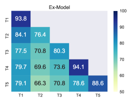
Baselines. We compare the following baselines and their details are shown in Tab. I. The architecture and implementation details are in Appendix A. The baselines are introduced as follows:

• Joint is a joint training method for all tasks on raw data. Since it does not involve the problem of forgetting, it is usually regarded as the upper bound of classic CL.

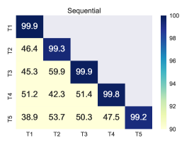
• Sequential represents the tasks encountered sequentially using the SGD optimizer to learn on the raw data stream. Since it does not have any strategies to alleviate forgetting, it is usually regarded as the lower bound for classic CL.

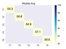
• Models-Avg directly averages the weights of all pre-trained models, requiring all APIs to have the same architecture and access to model parameters.

• Classic CL is the classic CL method, which learns directly from the raw data (in Fig. 1(a)). Without loss of generality, we exploit the classical replay-based approach (ER [11]).

• Ex-Model [7] is the CL from a stream of pre-trained white-box models, and it can be considered as the upper bound of our black-box API settings.

• DECL-APIs and DFCL-APIs are our proposed new settings for CL from a stream of black-box APIs with little or no raw data (as shown in Fig. 1(b)). We utilize the proposed data-free cooperative continual distillation learning framework to accomplish CL in both settings.

Metrics. We evaluate the performance of CL by measuring the average accuracy (ACC) and backward transfer (BWT). ACC measures the average accuracy of the CL model across all tasks, while BWT measures the degree of forgetting of the model. ACC and BWT are defined as follows:

$$\small ACC\!=\!\frac{1}{K}\sum_{i=1}^{K}A_{K,i},\;\;BWT\!=\!\frac{1}{K-1}\sum_{i=1}^{K-1}A_{K,i}\!-\!A_{i,i},$$

where $\small A_{k,i}$ represents the accuracy of the model tested on the task $\small i$ after the training of task $\small k$ is completed. $\small K$ denotes the number of tasks.

Figure 5: Layer-by-layer comparison of similarity on the trained network for the MNIST and SVHN.

Figure 6: Visualizations of real and synthetic data on the MNIST (a-b) and CIFAR-10 (c-d) datasets.

5.2 Results of Experiments on Same Model Architecture

Implementation. In this section, we assume that the API for all tasks in each dataset and the CL model use the same architecture. For the MNIST dataset, we use the LeNet5 [33] architecture, and for the SVHN, CIFAR10, CIFAR100 and MiniImageNet datasets, we use the ResNet18 [24] architecture. The network architectures of the generator, APIs, and CL model are defined in Appendix V. In addition, due to page limitations, detailed accuracies of all compared methods on the five datasets are provided in Appendix B.

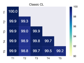
DFCL-APIs Performance. As shown in upper part of Tab. I and Tab. II, we have the following observations: (i) The Joint and Classic CL methods achieve the best performance as they are learned from all raw data. Among them, the Joint is superior to Classic CL because it assumes that all task data are available simultaneously, avoiding the problem of catastrophic forgetting. (ii) Sequential and Models-Avg are the worst-performing baseline methods. Sequential lack a mechanism to prevent catastrophic forgetting. Models-Avg averages the model parameters trained on tasks with different data distributions, leading to a drift between the averaged parameters and the optimal parameters of each task, resulting in poor performance. (iii) Ex-Model is a more practical approach that learns from a stream of pre-trained models without raw data, which achieved $\small 0.99\times$, $\small 0.98\times$, $\small 0.79\times$, $\small 0.53\times$ and $\small 0.40\times$ performance on MNIST, SVHN, CIFAR10, CIFAR100, MiniImageNet, respectively, compared to Classic CL. (iv) Our method achieves comparable performance to the upper bound Ex-Model on MNIST, SVHN, and CIFAR10 in DFCL-API setting. This is because our method generates more hard and diverse samples, and catastrophic forgetting is effectively alleviated. However, our approach is slightly inferior to Ex-Model on the more challenging CIFAR100 and MiniImageNet datasets, where both the number of tasks and classes significantly increased. This is due to the fact that Ex-Model had access to model parameters, whereas we could only use black-box API, and our settings are significantly more difficult.

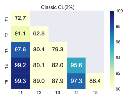
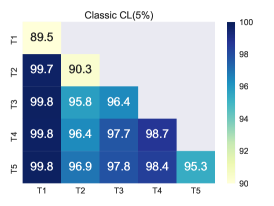
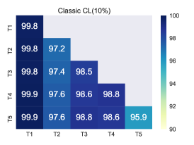
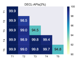
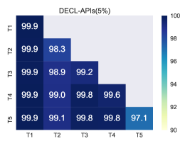
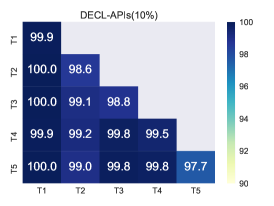
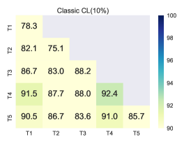
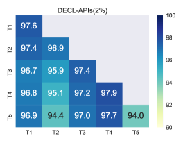
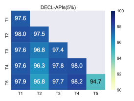
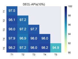
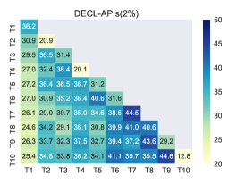
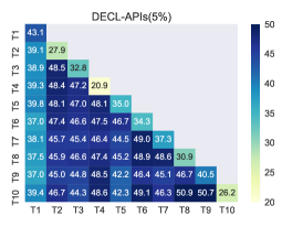
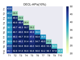
DECL-APIs Performance. As shown in the lower part of Tab. I and Tab. II, when a small amount of raw data ($\small 2\%,5\%,10\%$) is available, we have the following observations: (i) Classic CL performs poorly when there is only a small amount of raw task data. For example, considering the SVHN, CIFAR10, and CIFAR100 datasets and only having access to $\small 2\%$ of their raw data, the classic CL model can only achieve $\small 0.57\times$, $\small 0.79\times$, and $\small 0.43\times$ performance of the full data, respectively. (ii) When our method accesses only $\small 10\%$ of the data in the DECL-APIs setting, its performance far exceeds that of the DFCL-APIs setting. It achieves $\small 1.0\times$, $\small 0.97\times$, and $\small 0.75\times$ times the performance of classic CL on the three datasets SVHN, CIFAR10, and CIFAR100, respectively.

5.3 Results of Experiments on Heterogeneous Model Architectures

Implementation. As the architecture of APIs for different tasks may vary in practical applications, we tested only Ex-Model and our two settings, which are learned from pre-trained models, on CIFAR10 and CIFAR100. As shown in Tab. III, we use architectures with different depths (ResNet18$\rightarrow$ResNet34$\rightarrow$ResNet50), widths (ResNet$\rightarrow$WideResNet), and types (ResNet$\rightarrow$GoogleNet) for different APIs. We then learn from these APIs (For example, in Tab. III, CIFAR10 uses ResNet18 for task T1 and ResNet34 for task T2.) sequentially encountered under the three settings of Ex-Model, DFCL-APIs, and DECL-APIs, and we use ResNet18 as the architecture of the CL model. The network architectures are defined in Appendix V. In the DECL-APIs setting, we assume that $\small 10\%$ of the raw data is available.

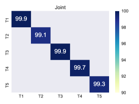
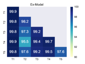
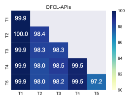
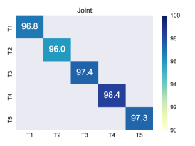
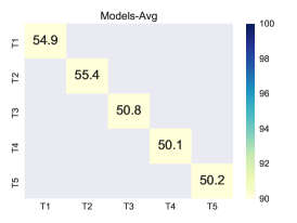
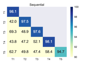
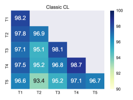
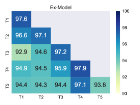
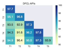
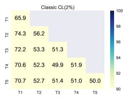
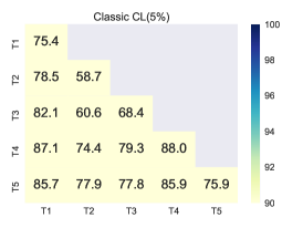
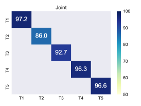
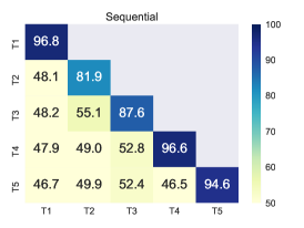
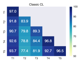
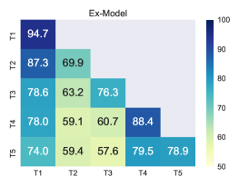
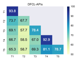
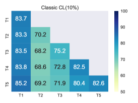
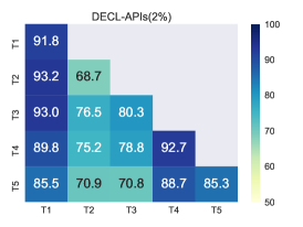
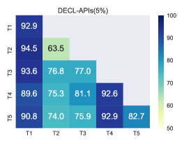
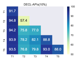
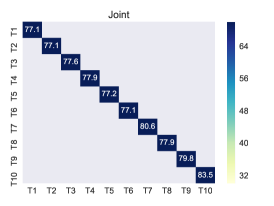
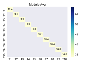
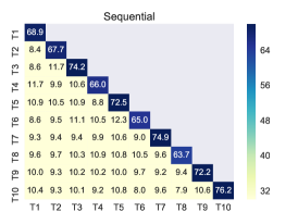
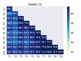
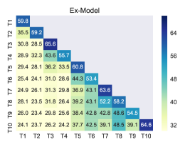
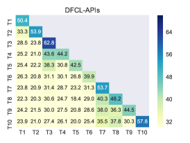
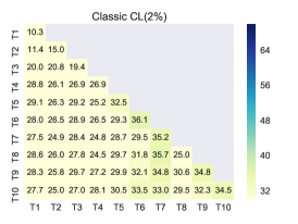
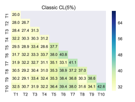
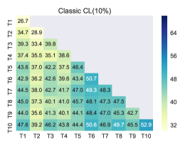
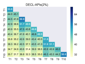
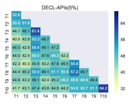
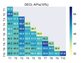
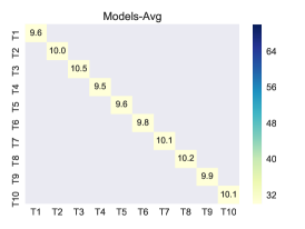
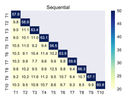
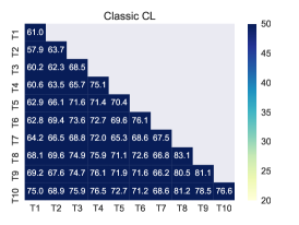
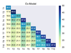
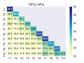
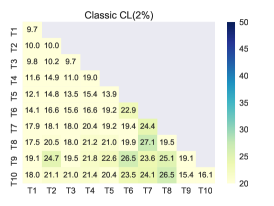
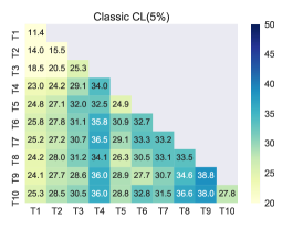
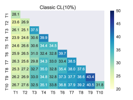
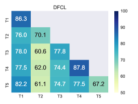
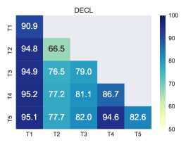
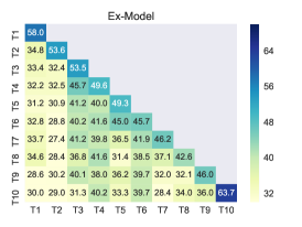
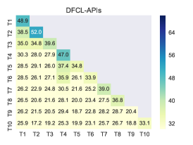
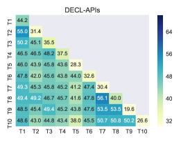
Tab. III shows the experimental results under the heterogeneous network. In addition, to observe the accuracy change and forgetting degree of each task in more detail during the training process, we provide the task accuracy of each stage on the CIFAR10 and CIFAR100 datasets in Fig. 3 and Fig. 4, respectively. We have the following observations: (i) On the CIFAR10 dataset, our method achieves performance close to that of Ex-Model under the DFCL-APIs setting, with the former being $\small 72.51\%$ and the latter being $\small 76.68\%$. Under the DECL-APIs setting, our method achieves a performance of $\small 86.42\%$. (ii) On the more challenging CIFAR100 dataset, there is a certain gap between DFCL-APIs and Ex-Model. This is because Ex-Model uses the pre-trained in a white-box manner, while DFCL-APIs access the black-box API. In DECL-APIs, our method has significantly improved performance. These results demonstrate that our method can also work with a stream of heterogeneous black-box APIs.

5.4 Ablation Study

Effectiveness of Each Component. In Sec. 4.2, we applied two regularization terms, Collaborative Generators and Class-balanced, to make the generated images diverse and evenly distributed in each class. In Sec. 4.3, we use Memory Replay and design a Network Similarity-based regularization strategies to avoid catastrophic forgetting. We verified the effectiveness of four components under the DFCL-APIs setting. As shown in Tab. IV, removing any single component leads to a drop in accuracy. For instance, on the CIFAR-10 dataset, removing the memory buffer and network similarity in the CL model part resulted in a drop from $\small 70.63\%$ to $\small 59.92\%$ and $\small 66.73\%$, respectively. The removal of the collaborative generators part and the class-balanced part led to a drop in ACC to $\small 67.50\%$ and $\small 69.75\%$, respectively. Removing all four components can result in a sharp drop in performance, with an ACC of only $\small 52.96\%$.

TABLE IV: Ablation study on MNIST, CIFAR10 and CIFAR100 datasets.

Variant	MNIST	CIFAR10	CIFAR100
DFCL-APIs (Ours)	98.58$\pm$0.41	70.63$\pm$6.03	30.52$\pm$1.51
w/o Memory Replay Loss	94.47$\pm$1.76	59.92$\pm$5.16	21.55$\pm$1.62
w/o Network Similarity Loss	98.48$\pm$0.20	66.73$\pm$2.72	26.79$\pm$2.26
w/o Cooperative Generators Loss	96.25$\pm$3.38	67.50$\pm$3.05	26.33$\pm$0.85
w/o Class-balanced Loss	98.52$\pm$0.54	69.75$\pm$1.46	25.70$\pm$1.68
w/o Four Losses	90.13$\pm$7.54	52.96$\pm$3.30	16.47$\pm$1.02

Network Similarity Analysis. The performance in Sec. 5.2 already illustrates the possibility of the proposed framework for CL without raw data. We further verify beyond accuracy on MNIST and SVHN datasets. We use the method of layer-by-layer similarity analysis (e.g., centered kernel alignment [47]) to observe whether the CL model trained by the proposed method without using raw data is highly similar to the CL model trained on raw data. As shown in Fig. 5, in the subfigures (a) and (c), we compare the similarity between two layers of the CL model trained on raw data and use it as the ground truth. In subfigures (b) and (d), we compare the similarity of the CL model trained on raw data to the CL model trained using pseudo data in the DFCL-APIs setting. We can observe that the values on the diagonal are significantly larger, i.e., the CL model trained on the DFCL-APIs setting is similar to the CL model trained on raw data.

Generated Samples Visualization. As shown in Fig. 6, we provide examples of real and generated images from the MNIST and CIFAR10 datasets, respectively. Our main goal in training generators in Sec. 4.2 is to create "hard" samples, rather than human-recognizable image details, so we cannot distinguish the corresponding classes of images. However, as we can see from the performance analysis, the generated images capture the main classification features of the raw task.

6 Conclusion

In this paper, we define two new CL settings: data-free continual learning (DFCL-APIs) and data-efficient continual learning (DECL), which executes CL from a stream of APIs with little or no raw data, respectively. To address the challenges in these two new settings, we propose a data-free cooperative continual learning framework that distills the knowledge of the black-box APIs into the CL model. The proposed method (i) does not require full raw data and avoids data privacy problems to some extent, (ii) does not require model architecture and parameters, (iii) only calls API and can adapt to API with any scale, and (iv) effectively alleviates catastrophic forgetting. Experimental results show that it is possible to conduct CL from API streams, which greatly expands the application of CL.

Appendix A Experiment Details

Dataset Statistics. We evaluate our method on MNIST [33], SVHN [42], CIFAR10 [30], CIFAR100 [30] and MiniImageNet [57] datasets. The dataset statistics are shown in Tab. V. Specifically, the column "#Classes" indicates how many classes are in each dataset. The column "#Tasks" indicates the number of continuously arriving tasks in the corresponding dataset. The columns "#Train", "#Valid", and "#Test" represent the average number of training, validation, and test samples in each task, respectively. The column "#Image Size" represents the resolution of each image in the raw dataset.

TABLE V: Statistics of the datasets.

Datasets	#Classes	#Tasks	#Train	#Valid	#Test	#Image Size
MNIST	10	5	10,800	1,200	2,000	1 $\times$ 28 $\times$ 28
SVHN	10	5	13,919	732	5,206	3 $\times$ 32 $\times$ 32
CIFAR10	10	5	9,500	500	2,000	3 $\times$ 32 $\times$ 32
CIFAR100	100	10	4,750	250	1,000	3 $\times$ 32 $\times$ 32
MiniImageNet	100	10	4,500	500	1,000	3 $\times$ 64 $\times$ 64

Architecture Details. We refer to the generators and commonly used network architectures defined by model extraction [56, 18, 27]. The architectures of generators and APIs are respectively defined as follows. (1) Generators: In all datasets and experiments, we use the network architecture shown in Tab. VI as generators. (2) APIs and CL Model: In the same architecture experiments in Sec. 5.2, the APIs and CL model of the MNIST dataset use the LeNet architecture shown in Tab. VII, and the APIs and CL model on the remaining four datasets use the ResNet18 architecture shown in Tab. VIII. In the heterogeneous architecture experiments in Sec. 5.3, the CL model uses the ResNet18 architecture, and different APIs use different network architectures (in Tab. III). The architectures involved in ResNet18, ResNet34, ResNet50, WideResNet, and GoogleNet are defined in Tables VIII, IX, X, XI, and XII, respectively.

TABLE VI: Generator Architecture.

Layer/Block	Configuration
Input	img_size, latent_dim, channels
FC Layer	Linear(latent_dim, 128 $\times$ (img_size // 4)2)
Block 1	BatchNorm2d(128)
Block 2	Conv2d(128, 128, 3, stride=1, padding=1)
	BatchNorm2d(128, 0.8)
	LeakyReLU(0.2, inplace=True)
Block 3	Conv2d(128, 64, 3, stride=1, padding=1)
	BatchNorm2d(64, 0.8)
	LeakyReLU(0.2, inplace=True)
	Conv2d(64, channels, 3, stride=1, padding=1)
	Tanh()
	BatchNorm2d(channels, affine=False)
Output	channels $\times$ img_size $\times$ img_size

TABLE VII: LeNet Architecture.

Layer/Block	Configuration
Input	channels, img_size, cls
Block 1	Conv2d(1, 6, kernel_size=(5, 5))
	ReLU()
	MaxPool2d(kernel_size=(2, 2), stride=2)
Block 2	Conv2d(6, 16, kernel_size=(5, 5))
	ReLU()
	MaxPool2d(kernel_size=(2, 2), stride=2)
Block 3	Conv2d(16, 120, kernel_size=(5, 5))
	ReLU()
FC Layer	Linear(120, 84)
	ReLU()
Output	Linear(84, cls)

TABLE VIII: ResNet18 Architecture.

Layer/Block	Configuration
Input	channel, in_planes, cls
Conv Layer	Conv2d(channal, 64, kernel_size=3, stride=1, padding=1, bias=False)
	BatchNorm2d(64)
Block 1	BasicBlock() $\times$ 2
Block 2	BasicBlock() $\times$ 2
Block 3	BasicBlock() $\times$ 2
Block 4	BasicBlock() $\times$ 2
Output	Linear(512 $\times$ 4, cls)
BasicBlock()	Conv2d(in_planes, planes, kernel_size=3, stride=stride, padding=1, bias=False)
	BatchNorm2d(planes)
	Relu()
	Conv2d(planes, planes, kernel_size=3, stride=1, padding=1, bias=False)
	BatchNorm2d(planes)
	Relu()

TABLE IX: ResNet34 Architecture.

Layer/Block	Configuration
Input	channel, in_planes, cls
Conv Layer	Conv2d(channal, 64, kernel_size=3, stride=1, padding=1, bias=False)
	BatchNorm2d(64)
Block 1	BasicBlock() $\times$ 3
Block 2	BasicBlock() $\times$ 4
Block 3	BasicBlock() $\times$ 6
Block 4	BasicBlock() $\times$ 3
Output	Linear(512 $\times$ 4, cls)
BasicBlock()	Conv2d(in_planes, planes, kernel_size=3, stride=stride, padding=1, bias=False)
	BatchNorm2d(planes)
	Relu()
	Conv2d(planes, planes, kernel_size=3, stride=1, padding=1, bias=False)
	BatchNorm2d(planes)
	Relu()

TABLE X: ResNet50 Architecture.

Layer/Block	Configuration
Input	channel, in_planes, cls
Conv Layer	Conv2d(channal, 64, kernel_size=3, stride=1, padding=1, bias=False)
	BatchNorm2d(64)
Block 1	Bottleneck() $\times$ 3
Block 2	Bottleneck() $\times$ 4
Block 3	Bottleneck() $\times$ 6
Block 4	Bottleneck() $\times$ 3
Output	Linear(512 $\times$ 4, cls)
Bottleneck()	Conv2d(in_planes, planes, kernel_size=1, bias=False)
	BatchNorm2d(planes)
	Relu()
	Conv2d(planes, planes, kernel_size=3, stride=stride, padding=1, bias=False)
	BatchNorm2d(planes)
	Relu()
	Conv2d(planes, expansion $\times$ planes, kernel_size=1, bias=False)
	BatchNorm2d(planes)
	Relu()

TABLE XI: WideResNet (WRN_16_1) Architecture.

Layer/Block	Configuration
Input	dropout_rate, channel, cls, depth=16, widen_factor=1
	nChannels = [16, 16$\times$widen_factor, 32$\times$widen_factor, 64$\times$widen_factor]
Conv Layer	Conv2d(channel, nChannels[0], kernel_size=3, stride=1, padding=1, bias=False)
Block 1	NetworkBlock(n, nChannels[0], nChannels[1], block, 1, dropout_rate)
Block 2	NetworkBlock(n, nChannels[1], nChannels[2], block, 2, dropout_rate)
Block 3	NetworkBlock(n, nChannels[2], nChannels[3], block, 2, dropout_rate)
	BatchNorm2d(nChannels[3])
	ReLU(inplace=True)
	Avg_pool2d()
Output	Linear(512 $\times$ 4, cls)
NetworkBlock()	Input: in_planes, out_planes, stride, dropout_rate=0.0
	BatchNorm2d(in_planes)
	ReLU(inplace=True)
	Conv2d(in_planes, out_planes, kernel_size=3, stride=stride, padding=1, bias=False)
	BatchNorm2d(out_planes)
	ReLU(inplace=True)
	Conv2d(out_planes, out_planes, kernel_size=3, stride=1, padding=1, bias=False)
	Dropout(dropout_rate)

TABLE XII: GoogleNet Architecture.

Layer/Block	Configuration
Input	channel, cls
Conv Layer	BasicConv2d(channel, 192, kernel_size=3, stride=1, padding=1)
Block 1	Inception(192, 64, 96, 128, 16, 32, 32)
	Inception(256, 128, 128, 192, 32, 96, 64)
	MaxPool2d(3, stride=2, padding=1, ceil_mode=False)
Block 2	Inception(480, 192, 96, 208, 16, 48, 64)
	Inception(512, 160, 112, 224, 24, 64, 64)
	Inception(512, 128, 128, 256, 24, 64, 64)
	Inception(512, 112, 144, 288, 32, 64, 64)
	Inception(528, 256, 160, 320, 32, 128, 128)
	MaxPool2d(3, stride=2, padding=1, ceil_mode=False)
Block 3	Inception(832, 256, 160, 320, 32, 128, 128)
	Inception(832, 384, 192, 384, 48, 128, 128)
	AdaptiveAvgPool2d()
	Dropout(0.2)
Output	Linear(1024, cls)
Inception()	Input: in_channels, ch1x1, ch3x3red, ch3x3, ch5x5red, ch5x5, pool_proj
	BasicConv2d(in_channels, ch1x1, kernel_size=1)
	BasicConv2d(in_channels, ch3x3red, kernel_size=1)
	BasicConv2d(ch3x3red, ch3x3, kernel_size=3, padding=1)
	BasicConv2d(in_channels, ch5x5red, kernel_size=1)
	BasicConv2d(ch5x5red, ch5x5, kernel_size=3, padding=1)
	MaxPool2d(kernel_size=3, stride=1, padding=1, ceil_mode=True)
	BasicConv2d(in_channels, pool_proj, kernel_size=1)
BasicConv2d()	Input: in_channels, out_channels
	Conv2d(in_channels, out_channels, bias=False)
	BatchNorm2d(out_channels, eps=0.001)
	Relu()

Implementation Details. We use the SGD optimizer for the CL model and the Adam optimizer [28] for generators. In addition, we used an early stopping strategy to avoid overfitting. We run three random seeds for each method and report the mean and standard deviation. The hyperparameter configurations of all experimental methods are shown in Tab. XIII.

TABLE XIII: The hyperparameters for all baselines. The ‘MINI’ denotes the MiniImagenet dataset.

Methods	Hyperparameters
Joint	Initial learning rate : 0.01 (MNIST, SVHN, CIFAR10, CIFAR100, MINI);
	Epoch: 10 (MNIST), 100 (SVHN, CIFAR10, MINI), 200 (CIFAR100);
	Batch size: 64 (MNIST, CIFAR100, MINI), 128 (SVHN, CIFAR)
Sequential	Initial learning rate : 0.01 (MNIST, SVHN, CIFAR10, CIFAR100, MINI);
	Epoch: 10 (MNIST), 100 (SVHN, CIFAR10, MINI), 200 (CIFAR100);
	Batch size: 64 (MNIST, CIFAR100, MINI), 128 (SVHN, CIFAR10)
Classic CL	Initial learning rate : 0.01 (MNIST, SVHN, CIFAR10, CIFAR100, MINI);
	Epoch: 10 (MNIST), 100 (SVHN, CIFAR10, MINI), 200 (CIFAR100);
	Batch size: 64 (MNIST, CIFAR100, MINI), 128 (SVHN, CIFAR10);
	Memory buffer size: 5000 (MNIST, SVHN, CIFAR10, CIFAR100, MINI)
Ex-Model	Initial learning rate : 0.01 (MNIST, SVHN, CIFAR10, CIFAR100, MINI);
	Epoch: 10 (MNIST), 30 (SVHN), 50 (CIFAR10, CIFAR100, MINI);
	Inner step: 50 (MNIST, SVHN, CIFAR10, CIFAR100, MINI);
	Batch size: 32 (MNIST, SVHN, CIFAR10, CIFAR100, MINI);
	Maximum memory buffer size: 5000 (MNIST, SVHN, CIFAR10, CIFAR100, MINI);
	Generator step: 1 (MNIST, SVHN, CIFAR10, CIFAR100, MINI);
	CL step: 4 (MNIST, SVHN, CIFAR10, CIFAR100, MINI);
	Generators learning rate: 0.001 (MNIST, SVHN, CIFAR10, CIFAR100, MINI);
	Latent dimension: 100 (MNIST), 256 (SVHN, CIFAR10, CIFAR100, MINI)
DFCL-APIs	Initial learning rate : 0.01 (MNIST, SVHN, CIFAR10, CIFAR100, MINI);
&	Epoch: 10 (MNIST), 30 (SVHN), 50 (CIFAR10, CIFAR100, MINI);
DECL-APIs	Inner step: 50 (MNIST, SVHN, CIFAR10, CIFAR100, MINI);
	Batch size: 32 (MNIST, SVHN, CIFAR10, CIFAR100, MINI);
	Maximum memory buffer size: 5000 (MNIST, SVHN, CIFAR10, CIFAR100, MINI);
	Generators step: 1 (MNIST, SVHN, CIFAR10, CIFAR100, MINI);
	CL step: 4 (MNIST, SVHN, CIFAR10, CIFAR100, MINI);
	Generators learning rate: 0.001 (MNIST, SVHN, CIFAR10, CIFAR100, MINI);
	Latent dimension: 100 (MNIST), 256 (SVHN, CIFAR10, CIFAR100, MINI);
	Generators regularization coefficient: 1 (MNIST, SVHN, CIFAR10, CIFAR100, MINI);
	CL regularization coefficient: 1 (MNIST, SVHN, CIFAR10, CIFAR100, MINI);

Appendix B More Experiment Analysis

Query Cost Analysis. To transfer the knowledge of the pre-trained black-box API to the CL model, we need to input the generated image into the API for a query and obtain the output logits. In this part, we study the impact of different query costs on the accuracy of the CL model under the DFCL-APIs setting. In our method, four API queries are required for each sample in each Generator model training step; that is, two API queries are required for gradient estimation for each Generator, and we have two Generators. When training the CL model, the API must be queried once per sample in each step. Therefore, the total API query cost for each task training is $E\times S\times B\times(4\times N_{\mathcal{G}}+N_{f_{cl}})$, where $E$, $S$, and $B$ represent the number of epochs, steps, and batch size, respectively, and $N_{\mathcal{G}}$ and $N_{f_{cl}}$ represent the number of times the GAN models and the CL model are updated in each step.

The results are shown in Tab. XIV, We made the following observations: (i) As the query cost of each task increases, the final ACC gradually increases. For example, on the CIFAR100 dataset, the query cost increases from 128K to 256K and then to 640K, resulting in an increase in the final ACC from 27.75% to 28.87% and then to 30.52%. This is because the higher the query cost per task, the more comprehensive the knowledge exploration of the API will be. (ii) However, increasing the query cost to 1280K leads to a decrease in the final ACC. This is due to the problem of catastrophic forgetting in CL. When the new API performs many updates to the CL model, it leads to catastrophic forgetting of old tasks, which can be seen from the BWT metric. When the query cost is 256K, 640K, and 1280K, the degree of forgetting is 20.21%, 21.40%, and 25.13%, respectively. The above results suggest that in the field of CL, there is a need to balance the impact of new task plasticity and old task forgetting on the final performance. It should be mentioned that a large number of queries increases the financial cost of calling the API [41], so it also makes sense to explore how to reduce the cost of API queries, which is beyond the scope of this paper and will be left for the future work.

TABLE XIV: Analysis of API query cost (per task) on the MNIST, CIFAR10, and CIFAR100 datasets.

MNIST	Maximum Budget	12K	64K	128K	256K
	ACC (%)	94.86	96.75	98.58	96.41
	BWT (%)	23.28	00.16	-00.13	-00.26
CIFAR10	Maximum Budget	128K	256K	640K	1280K
	ACC (%)	67.72	68.03	70.63	67.99
	BWT (%)	-05.67	-03.53	-09.98	-12.11
CIFAR100	Maximum Budget	128K	256K	640K	1280K
	ACC (%)	27.75	28.87	30.52	29.27
	BWT (%)	-13.62	-20.21	-21.41	-22.57

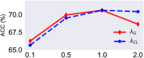
Hyperparameter Analysis. As shown in Fig. 7, we evaluate the performance sensitivity of our framework for different values of $\lambda_{G}$ and $\lambda_{CL}$ in Sec. 4.2 and Sec. 4.3 on CIFAR10, respectively. We observed that the two hyperparameters have similar trends. When the regularization strength is low, i.e., the hyperparameter value is small, the generated images may lack diversity or have class imbalance, and the CL model may suffer from catastrophic forgetting, resulting in poor performance. A better result can be obtained when the values of $\small\lambda_{G}$ and $\small\lambda_{CL}$ are set close to 1. We believe that further performance improvements can be achieved through finer tuning of the hyperparameters in the future.

Figure 7: Hyperparameter sensitivity analysis on CIFAR10 dataset.

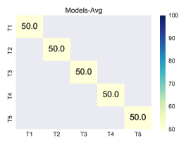
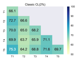
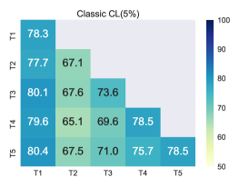
Accuracy Visualization. We provide the variation of the accuracy of each stage on the five datasets for all compared methods in Figures 8, 9, 10, 11, 12. We have the following conclusions: (i) Joint and Models-Avg are not a sequential learning process, so there is no catastrophic forgetting problem. (ii) Naive Sequential has a serious forgetting problem because there is no strategy to avoid forgetting. (iii) The Classic CL obviously alleviates catastrophic forgetting due to the experience replay mechanism. (iv) Both Ex-Model and DFCL-APIs perform slightly worse than Classic CL due to lack of original training data. In addition, since Ex-Model is a white box, it is the upper bound of DFCL-APIs. (v) In the setting of Classic CL and DECL-APIs with small amounts of data (i.e., $\small 2\%$, $\small 5\%$ and $\small 10\%$), the performance increases continuously with the amount of available data. In addition, DECL-APIs is superior to Classic CL because of the additional use of generated data.

Figure 8: The accuracy (Higher Better) on the MNIST dataset. (1) Joint, (2) Models-Avg, (3) Sequential, (4) Classic CL, (5) Ex-Model, (6) DFCL-APIs(ours), (7) Classic CL-2%, (8) Classic CL-5%, (9) Classic CL-10%, (10) DECL-APIs-2%(ours), (11) DECL-APIs-5%(ours), (12) DECL-APIs-10%(ours). $t$-th row represents the accuracy of the network tested on tasks $1-t$ after task $t$ is learned.

Figure 9: The accuracy (Higher Better) on the SVHN dataset. (1) Joint, (2) Models-Avg, (3) Sequential, (4) Classic CL, (5) Ex-Model, (6) DFCL-APIs(ours), (7) Classic CL-2%, (8) Classic CL-5%, (9) Classic CL-10%, (10) DECL-APIs-2%(ours), (11) DECL-APIs-5%(ours), (12) DECL-APIs-10%(ours). $t$-th row represents the accuracy of the network tested on tasks $1-t$ after task $t$ is learned.

Figure 10: The accuracy (Higher Better) on the CIFAR10 dataset. (1) Joint, (2) Models-Avg, (3) Sequential, (4) Classic CL, (5) Ex-Model, (6) DFCL-APIs(ours), (7) Classic CL-2%, (8) Classic CL-5%, (9) Classic CL-10%, (10) DECL-APIs-2%(ours), (11) DECL-APIs-5%(ours), (12) DECL-APIs-10%(ours). $t$-th row represents the accuracy of the network tested on tasks $1-t$ after task $t$ is learned.

Figure 11: The accuracy (Higher Better) on the CIFAR100 dataset. (1) Joint, (2) Models-Avg, (3) Sequential, (4) Classic CL, (5) Ex-Model, (6) DFCL-APIs(ours), (7) Classic CL-2%, (8) Classic CL-5%, (9) Classic CL-10%, (10) DECL-APIs-2%(ours), (11) DECL-APIs-5%(ours), (12) DECL-APIs-10%(ours). $t$-th row represents the accuracy of the network tested on tasks $1-t$ after task $t$ is learned.

Figure 12: The accuracy (Higher Better) on the MiniImageNet dataset. (1) Joint, (2) Models-Avg, (3) Sequential, (4) Classic CL, (5) Ex-Model, (6) DFCL-APIs(ours), (7) Classic CL-2%, (8) Classic CL-5%, (9) Classic CL-10%, (10) DECL-APIs-2%(ours), (11) DECL-APIs-5%(ours), (12) DECL-APIs-10%(ours). $t$-th row represents the accuracy of the network tested on tasks $1-t$ after task $t$ is learned.

References

- [1] Hongjoon Ahn, Sungmin Cha, Donggyu Lee, and Taesup Moon. Uncertainty-based continual learning with adaptive regularization. Advances in neural information processing systems, 32, 2019.
- [2] Ulrich Aïvodji, Sébastien Gambs, and Timon Ther. GAMIN: an adversarial approach to black-box model inversion. CoRR, abs/1909.11835, 2019.
- [3] Rahaf Aljundi, Francesca Babiloni, Mohamed Elhoseiny, Marcus Rohrbach, and Tinne Tuytelaars. Memory aware synapses: Learning what (not) to forget. In Computer Vision - ECCV 2018, volume 11207 of Lecture Notes in Computer Science, pages 144–161. Springer, 2018.
- [4] Rahaf Aljundi, Francesca Babiloni, Mohamed Elhoseiny, Marcus Rohrbach, and Tinne Tuytelaars. Memory aware synapses: Learning what (not) to forget. In Computer Vision - ECCV 2018 - 15th European Conference, volume 11207 of Lecture Notes in Computer Science, pages 144–161. Springer, 2018.
- [5] Tom Brown, Benjamin Mann, Nick Ryder, Melanie Subbiah, Jared D Kaplan, Prafulla Dhariwal, Arvind Neelakantan, Pranav Shyam, Girish Sastry, Amanda Askell, et al. Language models are few-shot learners. Advances in neural information processing systems, 33:1877–1901, 2020.
- [6] Pietro Buzzega, Matteo Boschini, Angelo Porrello, Davide Abati, and Simone Calderara. Dark experience for general continual learning: a strong, simple baseline. Advances in neural information processing systems, 33:15920–15930, 2020.
- [7] Antonio Carta, Andrea Cossu, Vincenzo Lomonaco, and Davide Bacciu. Ex-model: Continual learning from a stream of trained models. In 2022 IEEE/CVF Conference on Computer Vision and Pattern Recognition Workshops (CVPRW), pages 3789–3798. IEEE Computer Society, 2022.
- [8] Arslan Chaudhry, Puneet Kumar Dokania, Thalaiyasingam Ajanthan, and Philip H. S. Torr. Riemannian walk for incremental learning: Understanding forgetting and intransigence. In Proceedings of the European conference on computer vision (ECCV), pages 532–547. Springer, 2018.
- [9] Arslan Chaudhry, Albert Gordo, Puneet K. Dokania, Philip H. S. Torr, and David Lopez-Paz. Using hindsight to anchor past knowledge in continual learning. In Thirty-Fifth AAAI Conference on Artificial Intelligence, pages 6993–7001. AAAI Press, 2021.
- [10] Arslan Chaudhry, Naeemullah Khan, Puneet Dokania, and Philip Torr. Continual learning in low-rank orthogonal subspaces. Advances in Neural Information Processing Systems, 33:9900–9911, 2020.
- [11] Arslan Chaudhry, Marcus Rohrbach, Mohamed Elhoseiny, Thalaiyasingam Ajanthan, Puneet Kumar Dokania, Philip H. S. Torr, and Marc’Aurelio Ranzato. Continual learning with tiny episodic memories. CoRR, abs/1902.10486, 2019.
- [12] Hanting Chen, Tianyu Guo, Chang Xu, Wenshuo Li, Chunjing Xu, Chao Xu, and Yunhe Wang. Learning student networks in the wild. In Proceedings of the IEEE/CVF Conference on Computer Vision and Pattern Recognition, pages 6428–6437, 2021.
- [13] Hanting Chen, Yunhe Wang, Chang Xu, Zhaohui Yang, Chuanjian Liu, Boxin Shi, Chunjing Xu, Chao Xu, and Qi Tian. Data-free learning of student networks. In Proceedings of the IEEE/CVF International Conference on Computer Vision, pages 3514–3522, 2019.
- [14] Pin-Yu Chen, Huan Zhang, Yash Sharma, Jinfeng Yi, and Cho-Jui Hsieh. ZOO: zeroth order optimization based black-box attacks to deep neural networks without training substitute models. In Proceedings of the 10th ACM Workshop on Artificial Intelligence and Security, AISec@CCS 2017,, pages 15–26. ACM, 2017.
- [15] Andrew R Conn, Katya Scheinberg, and Luis N Vicente. Introduction to derivative-free optimization, volume 8 of MPS-SIAM series on optimization. SIAM, 2009.
- [16] Danruo Deng, Guangyong Chen, Jianye Hao, Qiong Wang, and Pheng-Ann Heng. Flattening sharpness for dynamic gradient projection memory benefits continual learning. In Advances in Neural Information Processing Systems 34: Annual Conference on Neural Information Processing Systems 2021, NeurIPS 2021, pages 18710–18721, 2021.
- [17] Prithviraj Dhar, Rajat Vikram Singh, Kuan-Chuan Peng, Ziyan Wu, and Rama Chellappa. Learning without memorizing. In Proceedings of the IEEE/CVF conference on computer vision and pattern recognition, pages 5138–5146, 2019.
- [18] Gongfan Fang, Jie Song, Chengchao Shen, Xinchao Wang, Da Chen, and Mingli Song. Data-free adversarial distillation. CoRR, abs/1912.11006, 2019.
- [19] Gongfan Fang, Jie Song, Xinchao Wang, Chengchao Shen, Xingen Wang, and Mingli Song. Contrastive model invertion for data-free knolwedge distillation. In Zhi-Hua Zhou, editor, Proceedings of the Thirtieth International Joint Conference on Artificial Intelligence, IJCAI-21, pages 2374–2380. International Joint Conferences on Artificial Intelligence Organization, 8 2021.
- [20] Mehrdad Farajtabar, Navid Azizan, Alex Mott, and Ang Li. Orthogonal gradient descent for continual learning. In The 23rd International Conference on Artificial Intelligence and Statistics, AISTATS 2020, volume 108 of Proceedings of Machine Learning Research, pages 3762–3773. PMLR, 2020.
- [21] Matt Fredrikson, Somesh Jha, and Thomas Ristenpart. Model inversion attacks that exploit confidence information and basic countermeasures. In Proceedings of the 22nd ACM SIGSAC Conference on Computer and Communications Security, pages 1322–1333. ACM, 2015.
- [22] Jonas Geiping, Hartmut Bauermeister, Hannah Dröge, and Michael Moeller. Inverting gradients - how easy is it to break privacy in federated learning? In Advances in Neural Information Processing Systems, 2020.
- [23] Jianping Gou, Baosheng Yu, Stephen J Maybank, and Dacheng Tao. Knowledge distillation: A survey. International Journal of Computer Vision, 129:1789–1819, 2021.
- [24] Kaiming He, Xiangyu Zhang, Shaoqing Ren, and Jian Sun. Deep residual learning for image recognition. In 2016 IEEE Conference on Computer Vision and Pattern Recognition, CVPR 2016, pages 770–778. IEEE Computer Society, 2016.
- [25] Christian Henning, Maria Cervera, Francesco D’Angelo, Johannes Von Oswald, Regina Traber, Benjamin Ehret, Seijin Kobayashi, Benjamin F Grewe, and João Sacramento. Posterior meta-replay for continual learning. Advances in Neural Information Processing Systems, 34:14135–14149, 2021.
- [26] Sanyam Kapoor, Theofanis Karaletsos, and Thang D Bui. Variational auto-regressive gaussian processes for continual learning. In International Conference on Machine Learning, pages 5290–5300. PMLR, 2021.
- [27] Sanjay Kariyappa, Atul Prakash, and Moinuddin K. Qureshi. MAZE: data-free model stealing attack using zeroth-order gradient estimation. In IEEE Conference on Computer Vision and Pattern Recognition, CVPR 2021, pages 13814–13823. Computer Vision Foundation / IEEE, 2021.
- [28] Diederik P. Kingma and Jimmy Ba. Adam: A method for stochastic optimization. In Yoshua Bengio and Yann LeCun, editors, 3rd International Conference on Learning Representations, ICLR 2015, 2015.
- [29] James Kirkpatrick, Razvan Pascanu, Neil Rabinowitz, Joel Veness, Guillaume Desjardins, Andrei A Rusu, Kieran Milan, John Quan, Tiago Ramalho, Agnieszka Grabska-Barwinska, et al. Overcoming catastrophic forgetting in neural networks. Proceedings of the national academy of sciences, 114(13):3521–3526, 2017.
- [30] Alex Krizhevsky, Geoffrey Hinton, et al. Learning multiple layers of features from tiny images. 2009.
- [31] Abhishek Kumar, Sunabha Chatterjee, and Piyush Rai. Bayesian structural adaptation for continual learning. In International Conference on Machine Learning, pages 5850–5860. PMLR, 2021.
- [32] Richard Kurle, Botond Cseke, Alexej Klushyn, Patrick Van Der Smagt, and Stephan Günnemann. Continual learning with bayesian neural networks for non-stationary data. In International Conference on Learning Representations, 2019.
- [33] Yann LeCun, Léon Bottou, Yoshua Bengio, and Patrick Haffner. Gradient-based learning applied to document recognition. Proceedings of the IEEE, 86(11):2278–2324, 1998.
- [34] Sen Lin, Li Yang, Deliang Fan, and Junshan Zhang. TRGP: trust region gradient projection for continual learning. In The Tenth International Conference on Learning Representations, ICLR. OpenReview.net, 2022.
- [35] Yuang Liu, Wei Zhang, Jun Wang, and Jianyong Wang. Data-free knowledge transfer: A survey. CoRR, abs/2112.15278, 2021.
- [36] David Lopez-Paz and Marc’Aurelio Ranzato. Gradient episodic memory for continual learning. In Advances in Neural Information Processing Systems, pages 6467–6476, 2017.
- [37] Aleksander Madry, Aleksandar Makelov, Ludwig Schmidt, Dimitris Tsipras, and Adrian Vladu. Towards deep learning models resistant to adversarial attacks. In 6th International Conference on Learning Representations, ICLR 2018. OpenReview.net, 2018.
- [38] Arun Mallya, Dillon Davis, and Svetlana Lazebnik. Piggyback: Adapting a single network to multiple tasks by learning to mask weights. In Computer Vision - ECCV 2018 - 15th European Conference, Munich, Germany, September 8-14, 2018, Proceedings, Part IV, volume 11208 of Lecture Notes in Computer Science, pages 72–88. Springer, 2018.
- [39] Arun Mallya and Svetlana Lazebnik. Packnet: Adding multiple tasks to a single network by iterative pruning. In 2018 IEEE Conference on Computer Vision and Pattern Recognition, CVPR 2018, pages 7765–7773. Computer Vision Foundation / IEEE Computer Society, 2018.
- [40] Abhishek Mishra. Machine Learning in the AWS Cloud: Add Intelligence to Applications with Amazon SageMaker and Amazon Rekognition. John Wiley & Sons, 2019.
- [41] Takayuki Miura, Satoshi Hasegawa, and Toshiki Shibahara. MEGEX: data-free model extraction attack against gradient-based explainable AI. CoRR, abs/2107.08909, 2021.
- [42] Yuval Netzer, Tao Wang, Adam Coates, Alessandro Bissacco, Bo Wu, and Andrew Y Ng. Reading digits in natural images with unsupervised feature learning. 2011.
- [43] Tribhuvanesh Orekondy, Bernt Schiele, and Mario Fritz. Knockoff nets: Stealing functionality of black-box models. In IEEE Conference on Computer Vision and Pattern Recognition, CVPR 2019, pages 4954–4963. Computer Vision Foundation / IEEE, 2019.
- [44] Pingbo Pan, Siddharth Swaroop, Alexander Immer, Runa Eschenhagen, Richard Turner, and Mohammad Emtiyaz E Khan. Continual deep learning by functional regularisation of memorable past. Advances in Neural Information Processing Systems, 33:4453–4464, 2020.
- [45] Nicolas Papernot, Patrick McDaniel, Ian Goodfellow, Somesh Jha, Z Berkay Celik, and Ananthram Swami. Practical black-box attacks against machine learning. In ACM on Asia conference on computer and communications security, pages 506–519, 2017.
- [46] German Ignacio Parisi, Ronald Kemker, Jose L. Part, Christopher Kanan, and Stefan Wermter. Continual lifelong learning with neural networks: A review. Neural Networks, 113:54–71, 2019.
- [47] Maithra Raghu, Thomas Unterthiner, Simon Kornblith, Chiyuan Zhang, and Alexey Dosovitskiy. Do vision transformers see like convolutional neural networks? In Advances in Neural Information Processing Systems 34: Annual Conference on Neural Information Processing Systems 2021, NeurIPS 2021, pages 12116–12128, 2021.
- [48] Dumitru Roman, Sven Schade, AJ Berre, N Rune Bodsberg, and J Langlois. Model as a service (maas). In AGILE workshop: Grid technologies for geospatial applications, Hannover, Germany, 2009.
- [49] Gobinda Saha, Isha Garg, and Kaushik Roy. Gradient projection memory for continual learning. In 9th International Conference on Learning Representations, ICLR 2021, 2021.
- [50] Joan Serrà, Didac Suris, Marius Miron, and Alexandros Karatzoglou. Overcoming catastrophic forgetting with hard attention to the task. In Proceedings of the 35th International Conference on Machine Learning, ICML 2018, volume 80 of Proceedings of Machine Learning Research, pages 4555–4564. PMLR, 2018.
- [51] David Silver, Aja Huang, Chris J. Maddison, Arthur Guez, Laurent Sifre, George van den Driessche, Julian Schrittwieser, Ioannis Antonoglou, Vedavyas Panneershelvam, Marc Lanctot, Sander Dieleman, Dominik Grewe, John Nham, Nal Kalchbrenner, Ilya Sutskever, Timothy P. Lillicrap, Madeleine Leach, Koray Kavukcuoglu, Thore Graepel, and Demis Hassabis. Mastering the game of go with deep neural networks and tree search. Nature, 529(7587):484–489, 2016.
- [52] David Silver, Julian Schrittwieser, Karen Simonyan, Ioannis Antonoglou, Aja Huang, Arthur Guez, Thomas Hubert, Lucas Baker, Matthew Lai, Adrian Bolton, Yutian Chen, Timothy P. Lillicrap, Fan Hui, Laurent Sifre, George van den Driessche, Thore Graepel, and Demis Hassabis. Mastering the game of go without human knowledge. Nature, 550(7676):354–359, 2017.
- [53] Tianxiang Sun, Zhengfu He, Hong Qian, Yunhua Zhou, Xuanjing Huang, and Xipeng Qiu. Bbtv2: Towards a gradient-free future with large language models. In Proceedings of the 2022 Conference on Empirical Methods in Natural Language Processing, EMNLP 2022, pages 3916–3930. Association for Computational Linguistics, 2022.
- [54] Tianxiang Sun, Yunfan Shao, Hong Qian, Xuanjing Huang, and Xipeng Qiu. Black-box tuning for language-model-as-a-service. In International Conference on Machine Learning, ICML 2022, volume 162 of Proceedings of Machine Learning Research, pages 20841–20855. PMLR, 2022.
- [55] Christian Szegedy, Wei Liu, Yangqing Jia, Pierre Sermanet, Scott Reed, Dragomir Anguelov, Dumitru Erhan, Vincent Vanhoucke, and Andrew Rabinovich. Going deeper with convolutions. In CVPR, pages 1–9, 2015.
- [56] Jean-Baptiste Truong, Pratyush Maini, Robert J. Walls, and Nicolas Papernot. Data-free model extraction. In IEEE Conference on Computer Vision and Pattern Recognition, CVPR 2021, pages 4771–4780. Computer Vision Foundation / IEEE, 2021.
- [57] Oriol Vinyals, Charles Blundell, Timothy Lillicrap, Daan Wierstra, et al. Matching networks for one shot learning. pages 3630–3638, 2016.
- [58] Zhenyi Wang, Li Shen, Le Fang, Qiuling Suo, Tiehang Duan, and Mingchen Gao. Improving task-free continual learning by distributionally robust memory evolution. In International Conference on Machine Learning, ICML 2022, volume 162 of Proceedings of Machine Learning Research, pages 22985–22998. PMLR, 2022.
- [59] Zhenyi Wang, Xiaoyang Wang, Li Shen, Qiuling Suo, Kaiqiang Song, Dong Yu, Yan Shen, and Mingchen Gao. Meta-learning without data via wasserstein distributionally-robust model fusion. In Uncertainty in Artificial Intelligence, pages 2045–2055. PMLR, 2022.
- [60] Zhenyi Wang, Enneng Yang, Li Shen, and Heng Huang. A comprehensive survey of forgetting in deep learning beyond continual learning. arXiv preprint arXiv:2307.09218, 2023.
- [61] Enneng Yang, Li Shen, Zhenyi Wang, Shiwei Liu, Guibing Guo, and Xingwei Wang. Data augmented flatness-aware gradient projection for continual learning. In 2023 IEEE/CVF International Conference on Computer Vision, ICCV 2023. IEEE, 2023.
- [62] Ziqi Yang, Jiyi Zhang, Ee-Chien Chang, and Zhenkai Liang. Neural network inversion in adversarial setting via background knowledge alignment. In Proceedings of the 2019 ACM SIGSAC Conference on Computer and Communications Security, pages 225–240, 2019.
- [63] Jaehong Yoon, Eunho Yang, Jeongtae Lee, and Sung Ju Hwang. Lifelong learning with dynamically expandable networks. In 6th International Conference on Learning Representations, ICLR 2018. OpenReview.net, 2018.
- [64] Guanxiong Zeng, Yang Chen, Bo Cui, and Shan Yu. Continual learning of context-dependent processing in neural networks. Nature Machine Intelligence, 1(8):364–372, 2019.
- [65] Friedemann Zenke, Ben Poole, and Surya Ganguli. Continual learning through synaptic intelligence. In Proceedings of the 34th International Conference on Machine Learning, ICML, volume 70 of Proceedings of Machine Learning Research, pages 3987–3995. PMLR, 2017.
- [66] Xingjian Zhen, Zihang Meng, Rudrasis Chakraborty, and Vikas Singh. On the versatile uses of partial distance correlation in deep learning. In Computer Vision - ECCV 2022, volume 13686 of Lecture Notes in Computer Science, pages 327–346. Springer, 2022.