monthyearday\THEYEAR \monthname[\THEMONTH] \twodigit\THEDAY \newdateformatdaymonthyear\twodigit\THEDAY \monthname[\THEMONTH] \THEYEAR
Karhunen–Loève Data Imputation in High Contrast Imaging††thanks: FITS images are only available at the CDS via anonymous ftp to cdsarc.cds.unistra.fr (130.79.128.5) or via https://cdsarc.cds.unistra.fr/viz-bin/cat/J/A+A/
Detection and characterization of extended structures is a crucial goal in high contrast imaging. However, these structures face challenges in data reduction, leading to over-subtraction from speckles and self-subtraction with most existing methods. Iterative post-processing methods offer promising results, but their integration into existing pipelines is hindered by selective algorithms, high computational cost, and algorithmic regularization. To address this for reference differential imaging (RDI), here we propose the data imputation concept to Karhunen–Loève transform (DIKL) by modifying two steps in the standard Karhunen–Loève image projection (KLIP) method. Specifically, we partition an image to two matrices: an anchor matrix which focuses only on the speckles to obtain the DIKL coefficients, and a boat matrix which focuses on the regions of astrophysical interest for speckle removal using DIKL components. As an analytical approach, DIKL achieves high-quality results with significantly reduced computational cost ( orders of magnitude less than iterative methods). Being a derivative method of KLIP, DIKL is seamlessly integrable into high contrast imaging pipelines for RDI observations.
Key Words.:
(stars:) circumstellar matter – (Galaxies:) quasars: general – techniques: high angular resolution – techniques: image processing – methods: statistical1 Introduction
High contrast imaging aims at detecting and characterizing faint signals surrounding bright central sources (e.g., Oppenheimer & Hinkley, 2009; Benisty et al., 2023; Currie et al., 2023). To reach this goal, coronagraphs are used to suppress central light, and post-processing – combined with observational techniques – is implemented to remove residual light and speckles (e.g., Pueyo, 2018; Follette, 2023). With these setups, existing observational techniques and methods are efficiently detecting and characterizing point sources such as planets and brown dwarfs (e.g., Nielsen et al., 2019; Vigan et al., 2021), as well as circumstellar disks and quasar host galaxies in polarized light (e.g., Benisty et al., 2023; Gratadour et al., 2015). Total intensity detection for extended structures, however, is still prone to data reduction artifacts with most existing methods for ground-based observations (e.g., Ruane et al., 2019; Xie et al., 2022). Their characterization is limited by compromised data quality (e.g., Milli et al., 2012; Mazoyer et al., 2020; Olofsson et al., 2023; Xie et al., 2023).
To detect and characterize extended structures in total intensity, several statistics-based methods and their derivative methods are being used (e.g., Lafrenière et al., 2007; Soummer et al., 2012; Amara & Quanz, 2012; Ren et al., 2018, 2020; Pairet et al., 2018, 2021; Flasseur et al., 2021; Samland et al., 2021; Juillard et al., 2022; Berdeu et al., 2022). Nevertheless, these methods are either prone to severe overfitting that can alter the morphology and surface brightness of such structures (e.g., Lafrenière et al., 2007; Soummer et al., 2012), or being highly selective on reference regions and computationally intensive (e.g., Ren et al., 2018, 2020), or subject to regularization terms that may provide uncertain results on the morphology and surface brightness of extended structures (e.g., Flasseur et al., 2021; Pairet et al., 2021; Juillard et al., 2022). Meanwhile, a careful selection of data reduction regions (e.g., Galicher & Marois, 2011; Milli et al., 2012, 2017; Perrin et al., 2015) could provide better results than non-statistical methods, yet these regions need to be adjusted for different systems, and such a selection is challenging when the disk morphology is face-on, complex, or even unknown. Using non-negative matrix factorization (NMF: Lee & Seung, 2001), Ren et al. (2020) showed that data imputation with sequential NMF (DI-sNMF) could be a promising statistical method for simple disk morphology, and it can provide high-quality results with theoretically minimized signal alteration. However, the data imputation concept has only been applied in Ren et al. (2020) for NMF in high contrast imaging, and it can provide high-quality results only when some strict requirements are satisfied (e.g., Ren et al., 2020; Olofsson et al., 2023; Xie et al., 2023). What is more, DI-sNMF is computationally inefficient due to its iterative nature (e.g., Ren et al., 2018), calling for other analytical methods that can implement the data imputation concept.
In high contrast imaging, the principal-component-analysis-based Karhunen–Loève Image Projection (KLIP: Soummer et al., 2012; Amara & Quanz, 2012) method is one of the analytical method standards for data reduction. KLIP decomposes reference images into an orthogonal basis through Karhunen–Loève (KL) transform, and it has been included in post-processing pipelines (e.g., Wang et al., 2015; Gomez Gonzalez et al., 2016; Stolker et al., 2019; Lucas & Bottom, 2020). It is widely used by surveys on both exoplanets (e.g., Nielsen et al., 2019; Vigan et al., 2021) and circumstellar disks (e.g., Esposito et al., 2020; Xie et al., 2022; Cugno et al., 2023; Wallack et al., 2023). Due to its over-fitting nature (e.g., Soummer et al., 2012; Pueyo, 2016), KLIP encounters difficulty in detecting and characterizing complex and extended structures. While iterative KLIP derivatives (e.g. Pairet et al., 2018; Ginski et al., 2021; Stapper & Ginski, 2022) might help alleviate the over-subtraction and self-subtraction in certain observational setups, there are still persistent residual signals and self-subtraction artefacts that pose challenges to data interpretation. As a data replacement (i.e., imputation) attempt with KLIP, Hunziker et al. (2018) and Xuan et al. (2018) used KLIP-based background subtraction in an interpolation approach: first perform KL decomposition, then conduct KLIP while masking out the central regions. However, due to the masking of central regions, the KLIP procedure within were performed on a non-orthogonal basis. Such a KLIP treatment can introduce over-fitting, which is manifested as a higher empirical model for the background, and yields negative surrounding regions even before post-processing. Noticing this over-fitting, Xie et al. (2023) thus used DI-sNMF for background removal and post-processing to extract a double-spiraled system to enable precise spiral motion measurement. After all, a proper data imputation with KLIP would offer a promising way to produce high-quality results with a high computational efficiency.
In the upcoming era of Extremely Large Telescopes (ELTs), the reference differential imaging (RDI) observational setup, including star-hopping (Wahhaj et al., 2021), could likely dominate the observation modes to produce high-quality images of exoplanets, circumstellar disks, and quasar host galaxies (hereafter “astrophysical signals”) in total intensity. In an RDI observation, a reference star (or multiple reference stars), which does not host circumstellar signals, is used to empirically capture the point spread function and speckles of the target star or quasar to reveal the target’s astrophysical surroundings. With large collecting areas (e.g., Gilmozzi & Spyromilio, 2007), ELTs can reach high signal-to-noise ratios in a significantly smaller amount of time (e.g., Bowens et al., 2021) than existing telescopes. In comparison, it might be suboptimal for the classical angular differential imaging (ADI: Marois et al., 2006) observation setup to be deployed on ELTs, since ADI requires a sufficient amount of field rotation of the sky for data processing (e.g., Milli et al., 2012; Xuan et al., 2018), yet sky rotation rate is a natural phenomenon that cannot be changed. To reduce and process the ELT data with high fidelity in RDI observations, iteratively methods could be potentially offer the best results. However, these iterative methods might be limited due to their significantly high computational cost than analytical methods, especially when there are high-resolution observations with a large number of datasets. Therefore, an analytical RDI data reduction method is needed to provide high-quality results in an efficient way.
In this study, by engineering the mathematical basics for KLIP, we enable it with the data imputation concept (DIKL). By modifying two steps in the standard KLIP procedure, and illustrating the DIKL results, we expect DIKL to be a promising method in RDI data reduction. In comparison with the established iterative DI-sNMF method which offers high-quality RDI results (e.g., Olofsson et al., 2023; Xie et al., 2023), such modifications allow an analytical data imputation by DIKL. It is computationally more efficient than iterative methods such as DI-sNMF by orders of magnitude, and it can provide results with comparable quality as DI-sNMF in RDI datasets.
2 Method
In high contrast imaging observations which require the usage of coronagraphs and adaptive optics systems, light signals from a central object (e.g., star, quasar) received on the detectors are superimposed on the astrophysical signals (e.g., Pueyo, 2018; Follette, 2023). The goal of post-processing is to extract the faint astrophysical signals (e.g., exoplanets, circumstellar disk, host galaxy) that are hidden behind these bright signals of non-astrophysical origin (e.g., adaptive optics halo, speckles, thermal background). For simplicity, we refer all these non-astrophysical signals as “speckles” hereafter. For an image which contains astrophysical signals, we refer it as target . For a set of images that only contain speckle signals, we refer them as reference images .111A target can serve as a reference in scenarios such as ADI, in which astrophysical signals move with respect to speckles in different images. In post-processing, we use the reference images to obtain the representative features of the speckles, then remove these features from a target image to reveal astrophysical signals in the residuals.
2.1 Overview of KLIP
For a reference image array containing reference images each with pixels, we denote the array as . A column in contains a reference image that is converted to a one-dimensional column vector (e.g., concatenating all columns of one image). We note that the notations here follow that of statisticians and computer scientists, instead of existing publications by astronomers (e.g., Soummer et al., 2012; Pueyo, 2016), to enable an efficient delivery of messages to non-astronomy readers in coding. Specifically, we have the reference array , with for and for matrix transpose, where for .
For a target image, we can convert it to a column vector . To remove the speckles from the target image, a statistics-based post-processing method first transforms the reference array to obtain a basis. This basis contains the representative features of the reference array (i.e., components). We then remove the representative features from the target vector. After post-processing, astrophysical signals are expected to reside in the residual image from feature removal.
The KLIP algorithm in Soummer et al. (2012) is consisted of two steps: the Karhunen–Loève (KL) transform of the reference matrix to obtain the KL component basis, and the projection of the target vector on the KL basis. For KLIP, the columns in both and are zero-spatial-mean. To reveal the astrophysical signals, the KLIP projection is then removed from the target image. To distinguish the difference between KLIP and DIKL later in this work, here we denote the reference array for KLIP as matrix , with allowing for the selection of smaller regions in reference images. Similarly, we denote the target vector as in KLIP processing. With these notations, we review the KLIP procedure as follows.
In the KL transform step, for a reference array , its covariance matrix is real symmetric. The spectral decomposition of is
| (1) |
where is a diagonal matrix whose diagonal entries are the eigenvalues of with , and is an orthonormal matrix with its columns being the corresponding eigenvectors with . Left multiply Eq. (1) by and right multiply by , we have
where we now have diagonalized the covariance matrix. By defining
| (2) |
we have an orthogonal KL component basis . The columns of the KL basis can be divided by the corresponding square root of the eigenvalues (e.g., Soummer et al., 2012), and thus creating an orthonormal basis . While we do not adopt this normalization since it does not impact the following target modeling procedure in the datasets used later in this study, such a normalization (e.g., VIP: Gomez Gonzalez et al., 2016) might be necessary for other datasets.
In the KL projection step, for a given target image vector with zero-spatial-mean , we can project and remove the KL component to obtain the residual ,
| (3) |
where is the cutoff count of the KL components (Soummer et al., 2012), and
| (4) |
is a scalar with , which denotes the projection from the target onto the -th KL component of .
In the next step of this study, we will modify the KLIP procedure to introduce DIKL post-processing. To perform DIKL data reduction, we need to focus on different regions of the reference array . For the full reference array , we can reorder or duplicate certain of its rows to obtain two submatrices,
| (5) |
where , , with and . Selection matrices and are boolean, and they are used to select specific rows in to form and , respectively. For example, to select the -th row from and store it in the -th row of , we have (and otherwise). To be more informative on the naming conventions of the superscripts in Eq. (5), we refer the two selected matrices as an anchor matrix and a boat matrix . The anchor matrix covers the regions which only host speckle signals, and the boat matrix can host astrophysical signals (and it can also contain the anchor matrix, which is adopted in this study), see Fig. 1 for an illustration of the selected regions.
2.2 DIKL for Reference Differential Imaging
The DIKL method modifies KLIP in two aspects. Specifically, the DIKL components are constructed by applying the eigenvectors from the anchor matrix to the boat matrix , and the DIKL projection adopts the projection coefficient between anchor target and anchor KL basis .
On the one hand, DIKL modifies the KL transform in Eq. (2). The DIKL basis follows
| (6) |
where we now instead use the eigenvectors from to construct the DIKL basis for regions. Here we use the prime symbol for the DIKL basis to distinguish it from a normal KL basis for the reference matrix . In comparison, the KL basis for is , and it is not calculated nor used in this study.
On the other hand, we modify the KL projection in Eq. (3). For a target vector with zero-spatial-mean, DIKL uses the coefficients from Eq. (4) between and , then applies the coefficients to the DIKL basis in Eq. (6). Specifically, the residual image after DIKL projection is
| (7) |
where the last equation adopts the bra–ket convention for the purpose of demonstration and connection with existing studies (e.g., Soummer et al., 2012).
With the above procedure, Eqs. (6) and (7) establish the DIKL post-processing procedure, see Appendix A for a corresponding pseudocode and implementation instructions. On the one hand, there is no direct projection of onto the KL basis of , which ensures the non-overfitting of non-speckle signals for DIKL. On the other hand, the projection coefficient is obtained from where speckle-only signals are expected (in both the reference images and the target image). Both ensure that astrophysical signals in the boat regions of are not captured in the coefficients in Eq. (7), and thus it serves as the data imputation step for DIKL. In fact, DIKL only performs KL transform to the speckles in the anchor matrix in this work, which avoids the high variation of signals in the boat matrix (e.g., regions that are close to the coronagraph) to dominate the classical KL transform (which is performed on the entire image), see Fig. 1.
We note that, however, Eq. (6) is limited in the reduction of non-RDI data. For example, in ADI datasets, we need to mask out different pixels in an observation sequence (e.g., Milli et al., 2017; Ren et al., 2020) to focus on speckle-only signals, since angular diversity is used to capture the speckles in an ADI observation sequence. We can indeed calculate an element in the covariance matrix by focusing only on the pixels that are not masked out in a pair of reference images, and perform spectral decomposition in Eq. (1) to obtain the corresponding eigenvectors. However, we cannot yet construct a basis following Eq. (2) for KLIP, nor Eq. (6) for DIKL, since weights in the eigenvector matrix are assigned to data that are masked out (i.e., artificially “missing”) in the reference array . To apply DIKL to ADI datasets, we can interpolate the speckle-only signals for the masked out data (e.g., Perrin et al., 2015) or iteratively fill the missing data (e.g., Bailey, 2012) in for Eq. (6), yet such treatments beyond the current scope of this analytical study.
3 Application
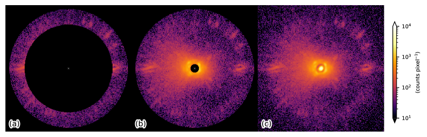
To demonstrate the DIKL method using on-sky RDI data, we retrieved datasets from the SPHERE instrument at the Very Large Telescope (VLT). We adopted data from IRDIS (Dohlen et al., 2008) of SPHERE in the star-hopping mode (Wahhaj et al., 2021). The star-hopping mode hops between a target star and its reference star during an observation sequence, thus reaching a quasi-simultaneous capture of speckle change. We retrieved the UT 2021-09-06, UT 2022-02-07, and UT 2022-04-01 observations of circumstellar disk hosts – HD 169142, PDS 201, and HD 129590 – as well as their reference stars from programs 105.209E and 105.20GP. We preprocess the data using the IRDAP pipeline (van Holstein et al., 2017, 2020), and the stars are then located at the center of the images. In the IRDIS data, with each IRDIS pixel having a spatial scale of mas (Maire et al., 2016), the control ring – interior to which the adaptive optics system can perform optimal dark hole correction to reveal faint objects – spans between pixel and pixel from the matrix centers. For further processing, we masked out the matrix elements that are interior to a radius of pixel from the center. We display the partitioning of an image in Fig. 1 for and illustration of the anchor region and the boat region in this study.
For the three groups of IRDIS datasets, the images for post-processing are the central pixel from the IRDAP preprocessed data. For one exposure, there are two channels from the preprocessed data, and we added them to produce one image. There are , , and target images, with , , and corresponding reference images, for HD 169142, PDS 201, and HD 129590, respectively. To convert a 2-dimensional image to a column in a matrix for this study, in practice, we created a 2-dimensional binary mask whose entries are 1 when the corresponding pixels are selected in Fig. 1(a)(b). For one image, we used the where function in numpy (Harris et al., 2020) to select the pixels in the images, and created a column for the selected matrix. By performing this for all reference images, we created the selected anchor matrix or the boat matrix for further post-processing. By performing this once for a target image, we created the selected anchor target vector or the boat target vector .
In post-processing, for the three IRDIS datasets that are in matrix form, we first followed Eq. (1) to perform spectral decomposition of the matrix elements in the anchor matrix (i.e., the IRDIS control ring). We then followed Eq. (6) to conduct DIKL transform on the boat matrix – the entire image (or the matrix elements interior to the outer edge of the control ring for the HD 129590 data) – using the eigenvectors from the covariance matrix of the anchor references. At last, to remove the speckles for a target image, we followed Eq. (7) to perform DIKL reduction, where we adopted the KLIP projection coefficients from Eq. (4) between the anchor target and anchor references. We reshaped the 1-dimensional vectors to 2-dimensional image, then derotated the reduction results for all target images to north-up and east-left according to their corresponding parallactic angles calculated using Pynpoint (Stolker et al., 2019). We calculated the element-wise median of the derotated reduction results as the combined image. We adopt the median-subtracted combined image as the final result.
3.1 Residual Variance
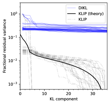
Variance of residual images can be informative of the existence of astrophysical signals. By performing DIKL on the reference images of the HD 169142 dataset, we generated the corresponding fractional residual variance (FRV) curves (e.g., Soummer et al., 2012; Ren et al., 2018). Specifically, for a reduced reference image, we divide its variance by that of the corresponding original image to generate the FRV. The FRV curves are then the FRV dependence as a function of KL components. Similarly, we generated the FRV curves for KLIP for comparison. For KLIP, FRV curves are expected to follow the fractional residual eigenvalues (Soummer et al., 2012), as can be seen in Fig. 2.
(The data used to create this figure are available in the ancillary folder on arXiv.)
(The data used to create this figure are available in the ancillary folder on arXiv.)
The FRV curves of DIKL converge to higher plateaus than those from KLIP. This convergence illustrates the less aggressive overfitting (or potentially non-overfitting of data; e.g., NMF: Ren et al., 2018) of DIKL. Similar as NMF, the FRV plateaus with DIKL is the indirect evidence that DIKL can retain more information of non-speckle signals than KLIP. In addition, the FRVs for DIKL reaches to stable values with DIKL components, suggesting that the rest of the components have negligible contribution in the DIKL process.
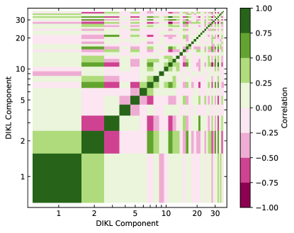
Due to the non-orthogonality of a DIKL basis, we witnessed a minor level of overfitting of the data, and thus we subtracted the median of the DIKL residuals to manually offset this effect. We present in Fig. 3 the correlation matrix for DIKL components: there exist crosstalks in the form of non-zero off-diagonal elements. However, given that the contribution of higher order DIKL components () are negligible in the FRVs in Fig. 2, the DIKL crosstalk only impacts the first few components, and the crosstalk does not contribute to data reduction beyond the first DIKL components due to the reaching of FRV plateaus in Fig. 2.
3.2 DIKL Imaging
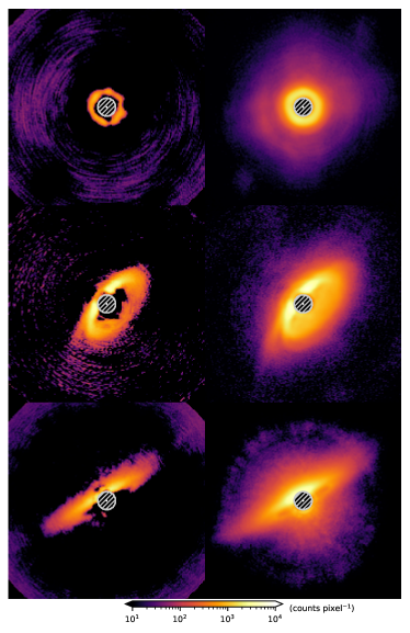
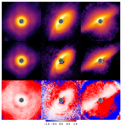
We used DIKL to reduce the star-hopping RDI observations of HD 169142, PDS 201, and HD 129590, which are known circumstellar disk hosts. The three disks have inclinations from nearly face-on to roughly edge-on (e.g., Pohl et al., 2017; Wagner et al., 2020; Matthews et al., 2017; Olofsson et al., 2023). We also reduced the datasets with KLIP and DI-sNMF for comparison.
Between the DIKL and KLIP results in Fig. 4, for the nearly face-on HD 169142, DIKL retrieves a two-ringed system, KLIP can nevertheless only recover the inner ring that is close to the coronagraph with compromised data quality. The DIKL result resembles the disk image obtained in polarized light, which thus demonstrates its superiority over KLIP in conserving face-on structures. Similarly, the PDS 201 and HD 129590 results have fine extended structures only seen in DIKL when compared with KLIP. In comparison, KLIP removes signals from the disks, altering disk morphology that poses challenges in data interpretation (e.g., Wagner et al., 2020; Olofsson et al., 2023).
(The data used to create this figure are available in the ancillary folder on arXiv.)
In comparison with the DI-sNMF method, which is mathematically well-founded to deliver high-quality results (e.g., Ren et al., 2020; Olofsson et al., 2023; Xie et al., 2023), DIKL can provide satisfactory results in Fig. 5. The DIKL results not only resemble the morphology of disks from DI-sNMF (Olofsson et al., 2023; Ren et al., 2023), but also agree with the DI-sNMF surface brightness values within for the disk-hosting regions. This further shows that DIKL can be a promising method in reaching high-quality results, and with a computational efficiency that is orders of magnitude better than DI-sNMF.
(The data used to create this figure are available in the ancillary folder on arXiv.)
With the demonstrated superiority of DIKL over the classical KLIP method in Fig. 4, as well as the consistency of its results with the established DI-sNMF method in Fig. 5, DIKL is a promising method that can produce high-quality results using similar amount of calculation time as KLIP. However, given that the DIKL basis being a non-orthogonal basis in practice, we should not yet ascribe full credibility in the fine details of DIKL results for interpretation until its application to datasets from other instruments is validated. Nevertheless, DIKL possesses a distinctive advantage in producing high-quality preliminary outcomes with high computational efficiency as the first step for data analysis. Such datasets with promising results can be then reduced with more advanced methods including DI-sNMF to ensure signal quality.
4 Summary
For RDI data reduction in high-contrast imaging, we demonstrated a high-efficiency and analytical approach to perform data imputation with modified KLIP algorithm: DIKL. Specifically, we can modify two steps in KLIP to reach the purpose of data imputation. On the one hand, in component construction, we use the eigenvectors of the covariance matrix – from the regions which only host speckle signals (i.e., the anchor matrix, “a”) – to generate the DIKL basis for the regions hosting non-speckle signals (i.e., the boat matrix, “b”), see Eq. (6). On the other hand, in speckle removal, we adopt the coefficients from capturing the speckles in the anchor matrix, and apply them to the DIKL basis and thus capture the speckles for the regions that host astrophysical signals in the boat matrix, see Eq. (7). With the two modifications, we only need to perform spectral decomposition once in Eq. (1). What is more, the corresponding covariance matrix for the anchor matrix is faster to compute than KLIP, due to a reduced number of matrix elements. As a result, the computational complexity of DIKL is similar as or less than that of KLIP.
By avoiding the projection of astrophysical signals onto speckle features, DIKL can recover face-on structures that are normally overfit in RDI observations, see Fig. 4. On the one hand, in comparison with the mathematically well-founded iterative DI-sNMF method in Ren et al. (2020), DIKL might potentially provide analytical results of low quality due to the non-orthogonal DIKL basis in Eq. (6). However, DIKL can approach a data quality similar to that of the latter in Fig. 5, since the crosstalk of the DIKL basis is negligible for higher order terms in Figs. 2 and 3. On the other hand, in comparison with the Hunziker et al. (2018) modification of KLIP, DIKL does not apply KL transform for the regions interior to the control ring while the latter does. Given that KL transform captures the variance of the signals (e.g., Soummer et al., 2012), while high contrast imaging observations have the highest variance next to the coronagraph (e.g., Pueyo, 2018), the Hunziker et al. (2018) and Xuan et al. (2018) approach should not be adopted to realize the data imputation concept for KLIP. In comparison with that approach, DIKL is not sensitive to such variances, since it uses the control ring signals that are less prone to random noise for KL transform, and thus DIKL is theoretically more plausible for data imputation. As a result, DIKL can be a promising analytical method that provides initial results, and with a orders of magnitude higher computational efficiency than the existing iterative methods (e.g., Ren et al., 2020). However, due to the crosstalk of DIKL basis, when the reference images are not stable, we recommend using DIKL for initial signal detection followed by other iterative data imputation methods for detailed characterization.
Given that DIKL is a natural extension of the KLIP algorithm, it can be implemented in the existing high-contrast imaging packages (e.g., Wang et al., 2015; Gomez Gonzalez et al., 2016; Stolker et al., 2019; Lucas & Bottom, 2020) for reference differential imaging data reduction. What is more, DIKL can perform data reduction for images containing negative values (from background removal), and thus it might potentially extract fainter disks than DI-sNMF which only takes in non-negative values. In the upcoming ELT era, we expect DIKL and its future derivative methods to provide high-quality results with high computational efficiency. Moving forward, on the one hand, we can assign different weights to the pixels in KL transform (e.g., Bailey, 2012) to make it less prone to random noise or shot noise. On the other hand, for non-RDI data (e.g., angular differential imaging, spectral differential imaging), more careful derivations which can handle missing data for different regions from different images, including modifying the covariance matrix for KL transform and the KLIP procedure, are needed in the future.
Acknowledgements.
We thank the anonymous referee for their suggestions that increased the readability and clarity of this manuscript, Mamadou N’Diaye for discussions, and Chen Xie for discussions on reference differential imaging in the ELT era. Based on observations collected at the European Organisation for Astronomical Research in the Southern Hemisphere under ESO programmes 105.209E and 105.20GP. We thank the PIs for the two programs (M. Benisty and J. Olofsson) for the datasets that validated this study. This research has received funding from the European Union’s Horizon 2020 research and innovation programme under the Marie Skłodowska-Curie grant agreement No. 101103114.References
- Amara & Quanz (2012) Amara, A., & Quanz, S. P. 2012, \hrefhttp://dx.doi.org/10.1111/j.1365-2966.2012.21918.xMNRAS, \hrefhttps://ui.adsabs.harvard.edu/abs/2012MNRAS.427..948A427, \hrefhttps://ui.adsabs.harvard.edu/abs/2012MNRAS.427..948A948
- Bailey (2012) Bailey, S. 2012, \hrefhttp://dx.doi.org/10.1086/668105PASP, \hrefhttps://ui.adsabs.harvard.edu/abs/2012PASP..124.1015B124, \hrefhttps://ui.adsabs.harvard.edu/abs/2012PASP..124.1015B1015
- Benisty et al. (2023) Benisty, M., Dominik, C., Follette, K., et al. 2023, \hrefhttp://dx.doi.org/10.48550/arXiv.2203.09991Astronomical Society of the Pacific Conference Series, \hrefhttps://ui.adsabs.harvard.edu/abs/2023ASPC..534..605B534, \hrefhttps://ui.adsabs.harvard.edu/abs/2023ASPC..534..605B605
- Berdeu et al. (2022) Berdeu, A., Langlois, M., & Vachier, F. 2022, \hrefhttp://dx.doi.org/10.1051/0004-6361/202142623A&A, \hrefhttps://ui.adsabs.harvard.edu/abs/2022A&A…658L…4B658, \hrefhttps://ui.adsabs.harvard.edu/abs/2022A&A…658L…4BL4
- Bowens et al. (2021) Bowens, R., Meyer, M. R., Delacroix, C., et al. 2021, \hrefhttp://dx.doi.org/10.1051/0004-6361/202141109A&A, \hrefhttps://ui.adsabs.harvard.edu/abs/2021A&A…653A…8B653, \hrefhttps://ui.adsabs.harvard.edu/abs/2021A&A…653A…8BA8
- Cugno et al. (2023) Cugno, G., Pearce, T. D., Launhardt, R., et al. 2023, \hrefhttp://dx.doi.org/10.1051/0004-6361/202244891A&A, \hrefhttps://ui.adsabs.harvard.edu/abs/2023A&A…669A.145C669, \hrefhttps://ui.adsabs.harvard.edu/abs/2023A&A…669A.145CA145
- Currie et al. (2023) Currie, T., Biller, B., Lagrange, A., et al. 2023, \hrefhttp://dx.doi.org/10.48550/arXiv.2205.05696Astronomical Society of the Pacific Conference Series, \hrefhttps://ui.adsabs.harvard.edu/abs/2023ASPC..534..799C534, \hrefhttps://ui.adsabs.harvard.edu/abs/2023ASPC..534..799C799
- Dohlen et al. (2008) Dohlen, K., Langlois, M., Saisse, M., et al. 2008, \hrefhttp://dx.doi.org/10.1117/12.789786Proc. SPIE, \hrefhttps://ui.adsabs.harvard.edu/abs/2008SPIE.7014E..3LD7014, \hrefhttps://ui.adsabs.harvard.edu/abs/2008SPIE.7014E..3LD70143L
- Esposito et al. (2020) Esposito, T. M., Kalas, P., Fitzgerald, M. P., et al. 2020, \hrefhttp://dx.doi.org/10.3847/1538-3881/ab9199AJ, \hrefhttps://ui.adsabs.harvard.edu/abs/2020AJ….160…24E160, \hrefhttps://ui.adsabs.harvard.edu/abs/2020AJ….160…24E24
- Flasseur et al. (2021) Flasseur, O., Thé, S., Denis, L., et al. 2021, \hrefhttp://dx.doi.org/10.1051/0004-6361/202038957A&A, \hrefhttps://ui.adsabs.harvard.edu/abs/2021A&A…651A..62F651, \hrefhttps://ui.adsabs.harvard.edu/abs/2021A&A…651A..62FA62
- Follette (2023) Follette, K. B. 2023, \hrefhttps://arxiv.org/abs/2308.01354arXiv, \hrefhttps://ui.adsabs.harvard.edu/abs/2023arXiv230801354FarXiv:2308.01354
- Galicher & Marois (2011) Galicher, R., & Marois, C. 2011, \hrefhttps://ui.adsabs.harvard.edu/abs/2011aoel.confP..25GP25
- Gilmozzi & Spyromilio (2007) Gilmozzi, R., & Spyromilio, J. 2007, The Messenger, \hrefhttps://ui.adsabs.harvard.edu/abs/2007Msngr.127…11G127, \hrefhttps://ui.adsabs.harvard.edu/abs/2007Msngr.127…11G11
- Ginski et al. (2021) Ginski, C., Facchini, S., Huang, J., et al. 2021, \hrefhttp://dx.doi.org/10.3847/2041-8213/abdf57ApJ, \hrefhttps://ui.adsabs.harvard.edu/abs/2021ApJ…908L..25G908, \hrefhttps://ui.adsabs.harvard.edu/abs/2021ApJ…908L..25GL25
- Gomez Gonzalez et al. (2016) Gomez Gonzalez, C. A., Wertz, O., Christiaens, V., et al. 2016, VIP: Vortex Image Processing pipeline for high-contrast direct imaging of exoplanets, \hrefhttp://ascl.net/1603.003ASCL, \hrefhttps://ui.adsabs.harvard.edu/abs/2016ascl.soft03003G1603.003
- Gratadour et al. (2015) Gratadour, D., Rouan, D., Grosset, L., et al. 2015, \hrefhttp://dx.doi.org/10.1051/0004-6361/201526554A&A, \hrefhttps://ui.adsabs.harvard.edu/abs/2015A&A…581L…8G581, \hrefhttps://ui.adsabs.harvard.edu/abs/2015A&A…581L…8GL8
- Harris et al. (2020) Harris, C. R., Millman, K. J., van der Walt, S. J., et al. 2020, \hrefhttp://dx.doi.org/10.1038/s41586-020-2649-2Nature, \hrefhttps://ui.adsabs.harvard.edu/abs/2020Natur.585..357H585, \hrefhttps://ui.adsabs.harvard.edu/abs/2020Natur.585..357H357
- Hunziker et al. (2018) Hunziker, S., Quanz, S. P., Amara, A., & Meyer, M. R. 2018, \hrefhttp://dx.doi.org/10.1051/0004-6361/201731428A&A, \hrefhttps://ui.adsabs.harvard.edu/abs/2018A&A…611A..23H611, \hrefhttps://ui.adsabs.harvard.edu/abs/2018A&A…611A..23HA23
- Juillard et al. (2022) Juillard, S., Christiaens, V., & Absil, O. 2022, \hrefhttp://dx.doi.org/10.1051/0004-6361/202244402A&A, \hrefhttps://ui.adsabs.harvard.edu/abs/2022A&A…668A.125J668, \hrefhttps://ui.adsabs.harvard.edu/abs/2022A&A…668A.125JA125
- Lafrenière et al. (2007) Lafrenière, D., Marois, C., Doyon, R., et al. 2007, \hrefhttp://dx.doi.org/10.1086/513180ApJ, \hrefhttps://ui.adsabs.harvard.edu/abs/2007ApJ…660..770L660, \hrefhttps://ui.adsabs.harvard.edu/abs/2007ApJ…660..770L770
- Lee & Seung (2001) Lee, D. D., & Seung, H. S. 2001, in \hrefhttp://papers.nips.cc/paper/1861-algorithms-for-non-negative-matrix-factorization.pdfAdvances in Neural Information Processing Systems 13, ed. T. K. Leen, T. G. Dietterich, & V. Tresp (MIT Press), 556
- Lucas & Bottom (2020) Lucas, M., & Bottom, M. 2020, \hrefhttp://dx.doi.org/10.21105/joss.02843JOSS, \hrefhttps://ui.adsabs.harvard.edu/abs/2020JOSS….5.2843L5, \hrefhttps://ui.adsabs.harvard.edu/abs/2020JOSS….5.2843L2843
- Maire et al. (2016) Maire, A.-L., Langlois, M., Dohlen, K., et al. 2016, \hrefhttp://dx.doi.org/10.1117/12.2233013Proc. SPIE, \hrefhttps://ui.adsabs.harvard.edu/abs/2016SPIE.9908E..34M9908, \hrefhttps://ui.adsabs.harvard.edu/abs/2016SPIE.9908E..34M990834
- Marois et al. (2006) Marois, C., Lafrenière, D., Doyon, R., et al. 2006, \hrefhttp://dx.doi.org/10.1086/500401ApJ, \hrefhttps://ui.adsabs.harvard.edu/abs/2006ApJ…641..556M641, \hrefhttps://ui.adsabs.harvard.edu/abs/2006ApJ…641..556M556
- Matthews et al. (2017) Matthews, E., Hinkley, S., Vigan, A., et al. 2017, \hrefhttp://dx.doi.org/10.3847/2041-8213/aa7943ApJ, \hrefhttps://ui.adsabs.harvard.edu/abs/2017ApJ…843L..12M843, \hrefhttps://ui.adsabs.harvard.edu/abs/2017ApJ…843L..12ML12
- Mazoyer et al. (2020) Mazoyer, J., Arriaga, P., Hom, J., et al. 2020, \hrefhttp://dx.doi.org/10.1117/12.2560091Proc. SPIE, \hrefhttps://ui.adsabs.harvard.edu/abs/2020SPIE11447E..59M11447, \hrefhttps://ui.adsabs.harvard.edu/abs/2020SPIE11447E..59M1144759
- Milli et al. (2012) Milli, J., Mouillet, D., Lagrange, A. M., et al. 2012, \hrefhttp://dx.doi.org/10.1051/0004-6361/201219687A&A, \hrefhttps://ui.adsabs.harvard.edu/abs/2012A&A…545A.111M545, \hrefhttps://ui.adsabs.harvard.edu/abs/2012A&A…545A.111MA111
- Milli et al. (2017) Milli, J., Vigan, A., Mouillet, D., et al. 2017, \hrefhttp://dx.doi.org/10.1051/0004-6361/201527838A&A, \hrefhttps://ui.adsabs.harvard.edu/abs/2017A&A…599A.108M599, \hrefhttps://ui.adsabs.harvard.edu/abs/2017A&A…599A.108MA108
- Nielsen et al. (2019) Nielsen, E. L., De Rosa, R. J., Macintosh, B., et al. 2019, \hrefhttp://dx.doi.org/10.3847/1538-3881/ab16e9AJ, \hrefhttps://ui.adsabs.harvard.edu/abs/2019AJ….158…13N158, \hrefhttps://ui.adsabs.harvard.edu/abs/2019AJ….158…13N13
- Olofsson et al. (2023) Olofsson, J., Thébault, P., Bayo, A., et al. 2023, \hrefhttp://dx.doi.org/10.1051/0004-6361/202346097A&A, \hrefhttps://ui.adsabs.harvard.edu/abs/2023A&A…674A..84O674, \hrefhttps://ui.adsabs.harvard.edu/abs/2023A&A…674A..84OA84
- Oppenheimer & Hinkley (2009) Oppenheimer, B. R., & Hinkley, S. 2009, \hrefhttp://dx.doi.org/10.1146/annurev-astro-082708-101717ARA&A, \hrefhttps://ui.adsabs.harvard.edu/abs/2009ARA&A..47..253O47, \hrefhttps://ui.adsabs.harvard.edu/abs/2009ARA&A..47..253O253
- Pairet et al. (2018) Pairet, B., Cantalloube, F., & Jacques, L. 2018, \hrefhttps://arxiv.org/abs/1812.01333arXiv, \hrefhttps://ui.adsabs.harvard.edu/abs/2018arXiv181201333ParXiv:1812.01333
- Pairet et al. (2021) —. 2021, \hrefhttp://dx.doi.org/10.1093/mnras/stab607MNRAS, \hrefhttps://ui.adsabs.harvard.edu/abs/2021MNRAS.503.3724P503, \hrefhttps://ui.adsabs.harvard.edu/abs/2021MNRAS.503.3724P3724
- Perrin et al. (2015) Perrin, M. D., Duchene, G., Millar-Blanchaer, M., et al. 2015, \hrefhttp://dx.doi.org/10.1088/0004-637X/799/2/182ApJ, \hrefhttps://ui.adsabs.harvard.edu/abs/2015ApJ…799..182P799, \hrefhttps://ui.adsabs.harvard.edu/abs/2015ApJ…799..182P182
- Pohl et al. (2017) Pohl, A., Benisty, M., Pinilla, P., et al. 2017, \hrefhttp://dx.doi.org/10.3847/1538-4357/aa94c2ApJ, \hrefhttps://ui.adsabs.harvard.edu/abs/2017ApJ…850…52P850, \hrefhttps://ui.adsabs.harvard.edu/abs/2017ApJ…850…52P52
- Pueyo (2016) Pueyo, L. 2016, \hrefhttp://dx.doi.org/10.3847/0004-637X/824/2/117ApJ, \hrefhttps://ui.adsabs.harvard.edu/abs/2016ApJ…824..117P824, \hrefhttps://ui.adsabs.harvard.edu/abs/2016ApJ…824..117P117
- Pueyo (2018) —. 2018, Direct Imaging as a Detection Technique for Exoplanets, \hrefhttp://adsabs.harvard.edu/abs/2018haex.bookE..10P10
- Ren et al. (2023) Ren, B., Benisty, M., Ginksi, C., et al. 2023, A&A, under review
- Ren et al. (2020) Ren, B., Pueyo, L., Chen, C., et al. 2020, \hrefhttp://dx.doi.org/10.3847/1538-4357/ab7024ApJ, \hrefhttps://ui.adsabs.harvard.edu/abs/2020arXiv200100563R892, \hrefhttps://ui.adsabs.harvard.edu/abs/2020arXiv200100563R74
- Ren et al. (2018) Ren, B., Pueyo, L., Zhu, G. B., et al. 2018, \hrefhttp://dx.doi.org/10.3847/1538-4357/aaa1f2ApJ, \hrefhttps://ui.adsabs.harvard.edu/abs/2018ApJ…852..104R852, \hrefhttps://ui.adsabs.harvard.edu/abs/2018ApJ…852..104R104
- Ruane et al. (2019) Ruane, G., Ngo, H., Mawet, D., et al. 2019, \hrefhttp://dx.doi.org/10.3847/1538-3881/aafee2AJ, \hrefhttps://ui.adsabs.harvard.edu/abs/2019AJ….157..118R157, \hrefhttps://ui.adsabs.harvard.edu/abs/2019AJ….157..118R118
- Samland et al. (2021) Samland, M., Bouwman, J., Hogg, D. W., et al. 2021, \hrefhttp://dx.doi.org/10.1051/0004-6361/201937308A&A, \hrefhttps://ui.adsabs.harvard.edu/abs/2021A&A…646A..24S646, \hrefhttps://ui.adsabs.harvard.edu/abs/2021A&A…646A..24SA24
- Soummer et al. (2012) Soummer, R., Pueyo, L., & Larkin, J. 2012, \hrefhttp://dx.doi.org/10.1088/2041-8205/755/2/L28ApJ, \hrefhttps://ui.adsabs.harvard.edu/abs/2012ApJ…755L..28S755, \hrefhttps://ui.adsabs.harvard.edu/abs/2012ApJ…755L..28SL28
- Stapper & Ginski (2022) Stapper, L. M., & Ginski, C. 2022, \hrefhttp://dx.doi.org/10.1051/0004-6361/202142820A&A, \hrefhttps://ui.adsabs.harvard.edu/abs/2022A&A…668A..50S668, \hrefhttps://ui.adsabs.harvard.edu/abs/2022A&A…668A..50SA50
- Stolker et al. (2019) Stolker, T., Bonse, M. J., Quanz, S. P., et al. 2019, \hrefhttp://dx.doi.org/10.1051/0004-6361/201834136A&A, \hrefhttps://ui.adsabs.harvard.edu/abs/2019A&A…621A..59S621, \hrefhttps://ui.adsabs.harvard.edu/abs/2019A&A…621A..59SA59
- van Holstein et al. (2017) van Holstein, R. G., Snik, F., Girard, J. H., et al. 2017, \hrefhttp://dx.doi.org/10.1117/12.2272554Proc. SPIE, \hrefhttps://ui.adsabs.harvard.edu/abs/2017SPIE10400E..15V10400, \hrefhttps://ui.adsabs.harvard.edu/abs/2017SPIE10400E..15V1040015
- van Holstein et al. (2020) van Holstein, R. G., Girard, J. H., de Boer, J., et al. 2020, \hrefhttp://dx.doi.org/10.1051/0004-6361/201834996A&A, \hrefhttps://ui.adsabs.harvard.edu/abs/2020A&A…633A..64V633, \hrefhttps://ui.adsabs.harvard.edu/abs/2020A&A…633A..64VA64
- Vigan et al. (2021) Vigan, A., Fontanive, C., Meyer, M., et al. 2021, \hrefhttp://dx.doi.org/10.1051/0004-6361/202038107A&A, \hrefhttps://ui.adsabs.harvard.edu/abs/2021A&A…651A..72V651, \hrefhttps://ui.adsabs.harvard.edu/abs/2021A&A…651A..72VA72
- Wagner et al. (2020) Wagner, K., Stone, J., Dong, R., et al. 2020, \hrefhttp://dx.doi.org/10.3847/1538-3881/ab893fAJ, \hrefhttps://ui.adsabs.harvard.edu/abs/2020AJ….159..252W159, \hrefhttps://ui.adsabs.harvard.edu/abs/2020AJ….159..252W252
- Wahhaj et al. (2021) Wahhaj, Z., Milli, J., Romero, C., et al. 2021, \hrefhttp://dx.doi.org/10.1051/0004-6361/202038794A&A, \hrefhttps://ui.adsabs.harvard.edu/abs/2021A&A…648A..26W648, \hrefhttps://ui.adsabs.harvard.edu/abs/2021A&A…648A..26WA26
- Wallack et al. (2023) Wallack, N. L., Ruffio, J.-B., Ruane, G., et al. 2023, AJ, accepted
- Wang et al. (2015) Wang, J. J., Ruffio, J.-B., De Rosa, R. J., et al. 2015, pyKLIP: PSF Subtraction for Exoplanets and Disks, \hrefhttp://ascl.net/1506.001ASCL, \hrefhttps://ui.adsabs.harvard.edu/abs/2015ascl.soft06001W1506.001
- Xie et al. (2022) Xie, C., Choquet, E., Vigan, A., et al. 2022, \hrefhttp://dx.doi.org/10.1051/0004-6361/202243379A&A, \hrefhttps://ui.adsabs.harvard.edu/abs/2022A&A…666A..32X666, \hrefhttps://ui.adsabs.harvard.edu/abs/2022A&A…666A..32XA32
- Xie et al. (2023) Xie, C., Ren, B. B., Dong, R., et al. 2023, \hrefhttp://dx.doi.org/10.1051/0004-6361/202346305A&A, \hrefhttps://ui.adsabs.harvard.edu/abs/2023A&A…675L…1X675, \hrefhttps://ui.adsabs.harvard.edu/abs/2023A&A…675L…1XL1
- Xuan et al. (2018) Xuan, W. J., Mawet, D., Ngo, H., et al. 2018, \hrefhttp://dx.doi.org/10.3847/1538-3881/aadae6AJ, \hrefhttps://ui.adsabs.harvard.edu/abs/2018AJ….156..156X156, \hrefhttps://ui.adsabs.harvard.edu/abs/2018AJ….156..156X156
Appendix A Pseudocode for DIKL implementation
We present a pseudocode to implement DIKL in Algorithm 1. Specifically, we use the KL projection coefficient from Eq. (4), and apply it to the DIKL basis in Eq. (6), to obtain the DIKL projection. We then remove the DIKL projection from the target image to reveal the astrophysical signals in Eq. (7).
To implement a standalone DIKL function, we need two matrix operations – matrix multiplication and eigendecomposition – both are available in modern scientific programming languages. Alternatively, to implement DIKL in the field of high contrast imaging, we can use existing KLIP frameworks (e.g., pyKLIP: Wang et al., 2015, VIP: Gomez Gonzalez et al., 2016, Pynpoint: Stolker et al., 2019, ADI.jl: Lucas & Bottom, 2020), since there are only two additional commands (at the end of Algorithm 1) in addition to KLIP for RDI observations. There is one extra command to select specific regions to obtain the anchor and boat matrices, and this selection is available using the mask commands in existing frameworks.
In actual implementation, we recommend splitting Algorithm 1 into two functions for computational efficiency. One function performs KL and DIKL transforms, and returns both the KL basis from Eq. (2) and the DIKL basis from Eq. (6). The other uses the KL basis to generate the KL projection coefficients from Eq. (4) for target , then apply the coefficients to the DIKL basis to obtain the residuals in Eq. (7). In this way, we can use the same reference array for the RDI reduction of different targets using DIKL.
To implement DIKL on existing high contrast imaging pipelines, we detail the key modifications here. Specifically, in the KL transform we need the eigenvector matrix in Eq. (1), and thus such an output is needed when eigendecomposition is conducted (e.g., pyKLIP222https://bitbucket.org/pyKLIP/pyklip/src/ab0040da1ae442dce9503502fc92f1736615b37d/pyklip/klip.py\#lines-137, Pynpoint333https://github.com/PynPoint/PynPoint/blob/main/pynpoint/util/psf.py\#L86, and VIP444https://github.com/vortex-exoplanet/VIP/blob/v1.4.0/vip_hci/psfsub/svd.py\#L442C21); for adi.jl555https://github.com/JuliaHCI/ADI.jl/blob/main/src/pca.jl\#L46 where singular value decomposition is conducted, we can use the output directly. We can then multiply the boat reference matrix with the eigenvector matrix to obtain the DIKL basis in Eq. (6). At last, we multiply the KL projection coefficients from the pipelines for Eq. (4) with the DIKL basis , then obtain the residuals in Eq. (7) after DIKL projection.