Reinforcement learning for safety-critical control of an automated vehicle

Abstract

We present our approach for the development, validation and deployment of a data-driven decision-making function for the automated control of a vehicle. The decision-making function, based on an artificial neural network is trained to steer the mobile robot SPIDER towards a predefined, static path to a target point while avoiding collisions with obstacles along the path. The training is conducted by means of proximal policy optimisation (PPO), a state of the art algorithm from the field of reinforcement learning.
The resulting controller is validated using KPIs quantifying its capability to follow a given path and its reactivity on perceived obstacles along the path. The corresponding tests are carried out in the training environment. Additionally, the tests shall be performed as well in the robotics situation Gazebo and in real world scenarios. For the latter the controller is deployed on a FPGA-based development platform, the FRACTAL platform, and integrated into the SPIDER software stack.

I Introduction

In this work we aim to showcase the implementation, validation and deployment of a machine learning (ML) application in a safety critical system. For this purpose a data-driven decision-making function for the automated control of the mobile robot SPIDER is developed. It extends the capabilities of a Stanley-based path tracking controller which is already integrated in the SPIDER software stack to a reactive path tracking controller. Thus, if an obstacle along the path is perceived by the robot, an evasion maneuver to avoid a collision is initiated.

The function is composed of several function blocks (see section IV-A). Its decision-making block, i.e. the unit which is providing the controls to be applied to the vehicle, is based on an artificial neural network (ANN). For the training procedure of this ANN, a state of the art algorithm from the field of reinforcement learning (RL) is used - see section IV-B.

The focal point of this work is on investigating the preservation of safety relevant driving functions while executing the abovementioned decision-making function. Hence, a framework supporting on one hand the execution of computationally intense vehicle functions, and on the other hand allowing its safe execution has to be provided. This is where the SPIDER and the FRACTAL project come into play.

The SPIDER is a mobile HiL platform developed at the Virtual Vehicle Research GmbH. It is designed for the testing of autonomous driving functions in real-world conditions, e.g. on proving grounds, in an automated and reproducible manner. The integrated safety concept ensures the safety of test drives. The FRACTAL platform a FPGA-based development platform, and various components developed in the FRACTAL project enhance the already existing safety concept. This includes monitoring units and a diverse redundancy library. In addition, the integrated hardware accelerators make the platform suitable for the execution of functions with high computing effort.
Due to the open system design of the SPIDER, the FRACTAL platform can be integrated into the SPIDER system. To incorporate the decision-making function into the SPIDER software stack and to run it on the FRACTAL platform, it is integrated into an appropriate ROS 2 node. For the deployment of the ANN the open-source deep learning library EDDL is used.

I-A Related work

The scientific literature knows several non data-driven methods for the solution of the path tracking and obstacle avoidance problem. Some popular and well-known path tracking controllers are the “Pure pursuit controller”, the “Carrot chasing controller”, or the “Stanley controller” - for details we refer to [9], [20], [23] or [13]. Approaches for the design of obstacle avoidance controllers, such as the artificial potential field method, can be found in [22], [31], [17].
However, we decided to follow a ML approach to tackle the reactive path tracking task. The main reason for this decision is that it seemed us to be difficult to appropriately tune and coordinate a combined controller consisting of a path tracking and a collision avoidance component. In addition, a slim and efficient ML solution promises a low computational effort at runtime. Quoting [15], RL offers to robotics a framework and a set of tools for the design of sophisticated and hard-to-engineer behaviors. According to that, RL approaches are well suited to the problem. The application of RL methods for the automated control of vehicles is not new - the topic was already adressed by a variety of researchers. We refer in this regard to [8], [14], [29], [2], [5] and as well [19]. For the sake of completeness, we point out that there are also non machine learning based methods for solving the reactive path tracking problem. See for example [30], [10].

I-B Structure of the paper

This paper is structured as follows. In Section II the main building blocks of this work are presented. Section III gives the formulation of the problem. In Section IV the structure and functioning of the decision-making function is presented. Finally, in the remaining sections the results obtained are presented and discussed.

II Preliminaries

II-A SPIDER

The SPIDER (Smart Physical Demonstration and Evaluation Robot) is an autonomous robot prototype developed at Virtual Vehicle Research GmbH. It is a mobile HiL platform designed for the development and testing of autonomous driving functions. It allows reproducible testing of perception systems, vehicle software and control algorithms under real world conditions. Four individually controllable wheels enable almost omni-directional movement, enabling the SPIDER to precisely mimic the movements of target vehicles - see Figure 1.

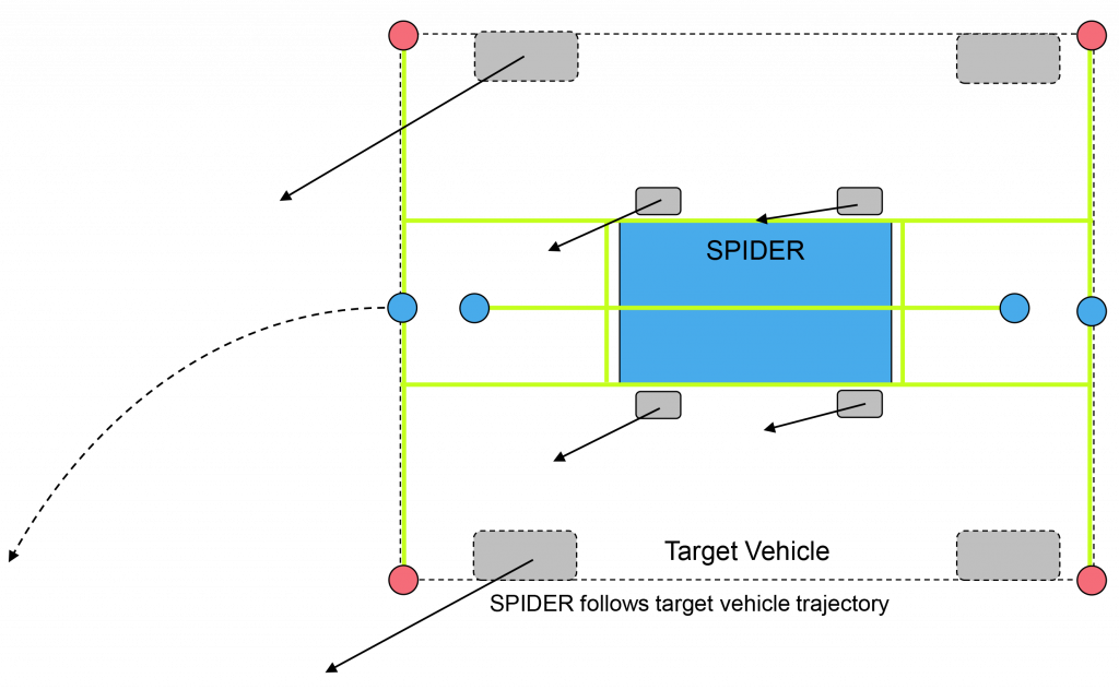
Figure 1: SPIDER following the trajectory of a target vehicle. The red dots indicate SPIDER sensors ensuring safety, where the blue dots correspond to sensors of the target vehicle. The green bars represent rods on which the sensors are mounted.

Due to its adaptable mounting rod system - see Figure 2 - positions of sensors can easily be adapted to the target system.

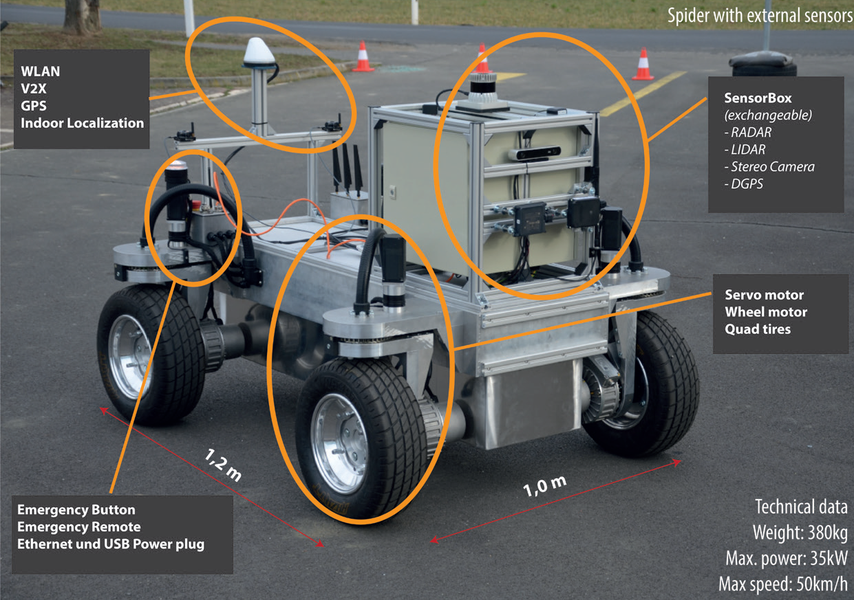
Figure 2: Smart Physical Demonstration and Evaluation Robot (SPIDER)

From a system perspective, the architecture of the SPIDER can be divided into three blocks, as shown in Figure 3. The decision-making function to be developed is located in the HLCU. Using the data provided by the sensor block, it determines control variables which are passed on to the LLCU in the form of a target linear speed and target angular velocity. The LLCU performs safety checks on these signals and forwards them to the corresponding hardware components.

Figure 3: System architecture of the SPIDER.

II-B The FRACTAL platform

The FRACTAL platform [18] is a new approach to reliable edge computing. It provides an Open-Safe-Reliable platform to build congnitive edge nodes while guaranteeing extra-functional properties like dependability, or security, as visualized in Figure 4. FRACTAL nodes can be deployed to various hardware architectures. The SPIDER use-case is deployed on a FPGA using the open-source SELENE hardware and software platform [11]. SELENE is a heterogeneous multicore processor platform based on the open RISC-V Instruction Set Architecture (ISA). The software stack is build on GNU/Linux. The SELENE platform is extended by various components from FRACTAL to ensure safety properties and allow the execution of computational extensive machine learning functions.

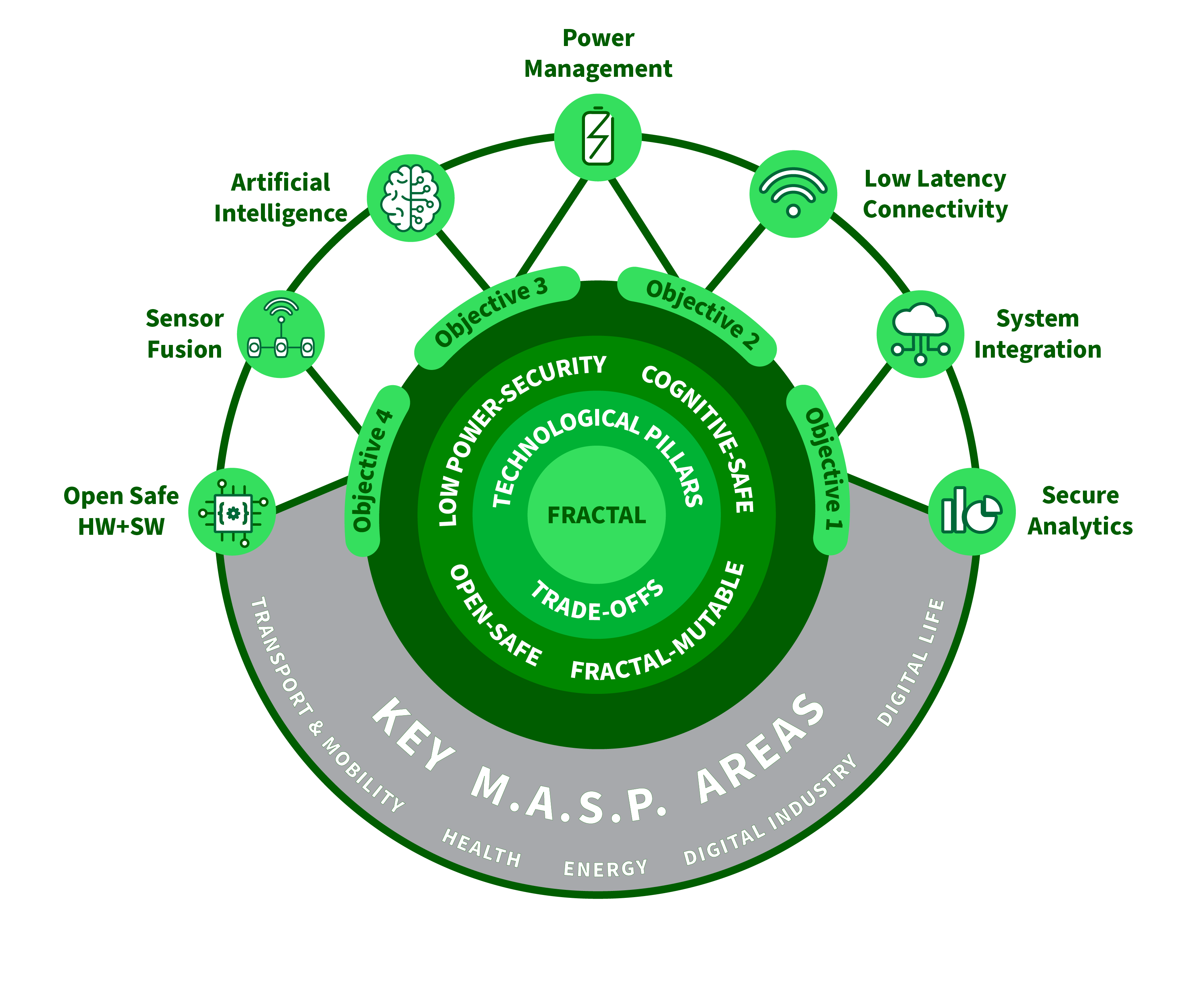
Figure 4: FRACTAL project technology pillars and objectives under the Multi-Annual Strategic Plan (”M.A.S.P.”)

The developments of SELENE and FRACTAL provide the baseline for the SPIDER to move from a non-safe industrial PC setup to an open source based, safe platform with smaller form-factor, and lower power comsumption. To add extra properties in context of safety and hardware acceleration, the SPIDER includes FRACTAL components on hardware and software level. This includes congestion detection at the memory controller, register file randomization, a redundant acceleration scheme, diverse redundancy of cores, and statistics units [1].

II-C Reinforcement learning

Reinforcement learning (RL) refers to a subarea of machine learning. The learning principle of methods belonging to this area is based on learning through interaction. Through repeated interaction with its environment, the learning system learns which actions are beneficial in terms of problem solving and which are detrimental in this respect. This is done by means of a numerical reward function tailored to the specific use case. By means of suitable optimization methods the system is encouraged to derive a control strategy, which, given a certain observation, selects the action that promises the maximum reward.
A more detailed description of the RL paradigm can be found for example in [15], [27].

II-D EDDL/LEDEL

The European Distributed Deep Learning Libray (EDDL) is a general-purpose deep learning library initially developed as part of the DeepHealth Toolkit [4] to cover deep learning needs in healthcare use cases within the DeepHealth project https://deephealth-project.eu/. The EDDL is a free and open-source software available on a GitHub repository https://github.com/deephealthproject/eddl/.

EDDL provides hardware-agnostic tensor operations to facilitate the development of hardware-accelerated deep learning functionalities and the implementation of the necessary tensor operators, activation functions, regularization functions, optimization methods, as well as all layer types (dense, convolutional and recurrent) to implement state-of-the-art neural network topologies. Given the requirement for fast computation of matrix operations and mathematical functions, the EDDL is being coded in C++. GPU specific implementations are based on the NVIDIA CUDA language extensions for C++. A Python API is also available in the same GitHub repository and known as pyEDDL.
In order to be compatible with existing developments and other deep learning toolkits, the EDDL uses ONNX [3], the standard format for neural network interchange, to import and export neural networks including both weights and topology.
In the Fractal project, the EDDL is being adapted to be executed on embedded and safety-critical systems. Usually, these systems are equipped with low resources, i.e., with limited memory and computing power, as it is the case of devices running on the edge.

When adapted to this kind of systems, the EDDL is renamed as Low Energy DEep Learning library (LEDEL).

Specifically, the EDDL has been ported to run on emulated environments based on the RISC-V CPU. It has been tested to train models and for inferencing. However, the use of the LEDEL in this work is only for inferencing, so that the running time is not a critical issue. The models are trained using the EDDL on powerful computers, then the trained models can be imported by the EDDL thanks to ONNX.

III Problem formulation

The decision-making function shall navigate the SPIDER along a predefined path from a starting point to a target point while avoiding collisions with obstacles.
Although the SPIDER can be controlled omnidirectionally, in this use case we limit ourselves to develop a car-like control strategy. As a consequence, reaching the target orientation at each of the given waypoints is disregarded.

IV Decision-making function

IV-A Design

The entire control unit is designed as depicted in Figure 5. At any time point it takes as input a cost map, the current state of the vehicle, the control values applied in the previous time step and provides the control values $(u_{1},u_{2})$ to be applied next as output. These values are sampled from the finite subset

$$U=\{(u_{1}, u_{2})~{}:~{}u_{1}=-0.5+1.5i/11,$$

$$u_{2}=-1+2j/11~{}1\leq i,j\leq 11\}.$$

of the control space $[-1/2,1]\times[-1,1]$ according to the probability distribution provided by the decision-making block represented through an ANN. Given the maximal linear acceleration $a_{max}$ and the maximal steering angle $\vartheta_{max}$ of the robot, the terms $u_{1}a_{max}$, $u_{2}\vartheta_{max}$ determine the acceleration and the steering angle respectively which will be applied to the vehicle.

We briefly discuss the main building blocks of the control unit next.

Figure 5: Decision-making flow

Range finding The range finding block consists of a module which takes as input a cost map of a fixed dimension centered around the vehicle and determines the distance from obstacles to the vehicle by means of a ray-casting approach. For this purpose, starting from the center of mass (COM) of the robot, $m$ virtual rays are plotted on the occupancy grid - see Figure 6. Along each of these arrows, the corresponding cell entry of the occupancy grid is checked at $n$ evenly distributed points, the so-called ray nodes. Based on the number of free cells counted from the inside to the outside, the distance (in meters) along a ray from the robot to any obstacles is determined.
It is assumed that the robot is entirely contained within a circular disk of radius $\rho_{1}$ centered at its COM. For the determination of the distances we thus only take in consideration ray nodes which are not contained in this disk. In addition the maximal distance is bounded by $\rho_{2}$. Thus we get distances in the interval $[0,\rho_{2}-\rho_{1}]$.

Figure 6: Illustration of the range finding procedure.

Reference segment selection To quantify the spatial proximity of the vehicle to the path the cross track error is used. By definition, the cross track error is the normal distance from the current position of the vehicle to the target trajectory. In the given context, it is determined as the normal distance of the position of the vehicle to the closest line segment which is connecting two consecutive waypoints. For the reference segment selection procedure we followed the apporach described in [7], Section 9.3.

ANN input generation The neural network takes $7$ input variables. Let $(x,y)$, $v$, $\theta$ denote the current position, the current linear speed and the current heading of the vehicle respectively. We denote by $u_{0}$ $u_{1}$ the control values, which were applied in the previous time step.

Let $k\in\mathbb{N}$ be such that the line segment $L_{(x,y)}$ determined by the reference segment selection procedure described above, connects the waypoints $w_{k},w_{k+1}$. Let $v_{k+1}$ denote the target velocity at $w_{k+1}$ and let $d=(d_{1},\ldots,d_{m})$ be the tuple of distances computed by the range finding unit given the current position of the vehicle. Then the input $x=(x_{1},\ldots,x_{7})$ to the neural network is defined as follows:

• Clipped cross track error: Let $e_{x}$ denote the signed normal distance of the vehicle’s position to $L_{(x,y)}$, i.e. $e_{x}$ defines the current cross track error. Given the clip parameter $\delta>0$, we define

  $$x_{1}=\begin{cases}-\delta,\textnormal{ if }e_{x}<-\delta\\ \delta,\textnormal{ if }e_{x}>\delta\\ e_{x},\textnormal{ else }\end{cases}$$

• Linear speed error: The linear speed error is defined as $x_{2}=v_{k+1}-v$.

• Waypoint heading error: We introduce the heading error $x_{3}$ as the cosine of the angle between the vector $v(\theta)$ indicating the driving direction of the vehicle and the vector connecting $w_{k}$ and $w_{k+1}$.

• Previous control values: Define $x_{4}=u_{0}$ and $x_{5}=u_{1}$.

• Obstacle heading error: We introduce $x_{6}$ to be the cosine of the angle between $v(\theta)$ and the range finding ray sensing the smallest distance to an obstacle.

• Smallest obstacle distance: Define $x_{7}$ to be the smallest distance to an object measured by the range finding unit.

We note that by these definitions the input variables of the neural network are always contained within a fixed range and are thus bounded. According to [26] such normalisation can accelerate and stabilise the training process.

Decision-making The ANN representing the decision-making block consists of two hidden dense layers of $64$ neurons each and an output layer of $|U|=121$ neurons. For the hidden layers $\tanh$ is used as activation function, whereas for the output layer the softmax function is used.

IV-B Training

For the training of the decision-making function we use the proximal policy optimisation (PPO) method presented in [24]. The training suite is implemented in Python and is built on the Python package Stable Baselines - see [12]. The driving environment which is used for the training procedure is based on the well known kinematic bicycle model, which is - according to [21] - a suitable and accurate model for car-like driving manoeuvres at low speeds.
The RL paradigm requires to choose a reward function adapted and aligned to the problem. In the given context it must be constructed in such a way that actions steering the vehicle with target speed along the target trajectory are rewarded. However, the rewarding approach must also reflect the collision avoidance requirement. Thus, actions which may lead to collisions must be penalised.

The approach we considered, builds on the work of [29], [5] and [19]. Its main lines are described next. The reward function $r$ is made up of a path following component $r_{pf}$ and a collision avoidance component $r_{ca}$. Given the input data $x=(x_{1},\ldots,x_{7})$ to the ANN, non-negative parameters $\alpha_{1},\ldots,\alpha_{4}$, $\beta_{1},\beta_{2}$, $\lambda$ we define

$$r_{1}(x)=\alpha_{1}\exp(-x_{1}^{2}/2\beta_{1})$$

$$r_{2}(x)=\alpha_{2}\exp(-x_{2}^{2}/2\beta_{2})$$

$$r_{3}(x)=\alpha_{3}x_{3}$$

With this we set

$$r_{pf}(x)=-1+(1+r_{2}(x)r_{3}(x))(1+r_{1}(x))$$

$$r_{ac}(x)=\begin{cases}-\alpha_{4}x_{6},\textnormal{ if }x_{7}\leq\lambda(\rho_{2}-\rho_{1})\\ 0,\textnormal{ else }\end{cases}$$

The definition of $r_{pf}$ implies, that large rewards can be achieved for small values of the cross track error, and small deviations from the target velocity and if the vehicle is approaching in a straight line the upcoming waypoint. Due to the additive constants in the definition of the reward function, driving strategies aligned only partially to the desired policy will not be disregarded. Thus, for example, deviations from the speed profile off the target trajectory result in positive rewards.

The definition of $r_{ac}$ on the other hand, punishes actions which steer the vehicle in the direction of the smallest distance to an obstacle. If the vehicle crashes into an obstacle an additional penalty $r_{crash}$ is applied. Combining $r_{ac}$, $r_{pf}$ and $r_{crash}$ via

$$r(x)=r_{ac}+r_{pf}+r_{crash}$$

we obtain a reward signal which honours actions that maximise the distance to obstacles and proximity to the path in the absence of obstacles in the vehicle’s surrounding.

V Evaluation and performance criteria

The validation of the decision-making function is based on KPIs. Two classes of KPIs are considered: KPIs for the assessment of the path tracking capability and KPIs for the assessment of the collision avoidance capability. For the validation we choose a specific path and a distribution of obstacles on or near the target trajectory. Let $(x_{1}^{(k)},x_{2}^{(k)},x_{3}^{(k)},x_{4}^{(k)},x_{5}^{(k)},x_{6}^{(k)},x_{7}^{(k)})_{0\leq k\leq N}$ denote the set of input terms to the ANN obtained by applying the decision-making function to the specified scenario in an episode of $N+1$ time steps.

V-A Path tracking

For the assessment of the path tracking performance we consider on the one hand the mean $l^{2}$ total tracking error $\kappa_{2}$ which is defined by

$$\kappa_{2}=\frac{1}{N}\sum_{k=1}^{N}\|(x_{1}^{(k)},x_{2}^{(k)})\|_{2}^{2}.$$

In addition we measure the path tracking capability of the decision-making function by means of the waypoint reach rate $\kappa_{reach}$: Consider a tuple $(z_{1},\ldots,z_{L})$ of points on the target trajectory arranged from the starting point towards the terminal point. Then $\kappa_{reach}$ is defined to be the quotient of the number of points $z_{l}$, $1\leq l\leq L$ which could be approximately reached in successive manner and the total number $L$ of points considered.

V-B Collision avoidance

To validate the collision avoidance capabilites of the decision-making function we use the metrics $\kappa_{danger}$ and $\kappa_{dist}$. The latter is defined by means of

$$\kappa_{dist}=\min\{x_{7}^{(k)}~{}:~{}0\leq k\leq N\}.$$

We emphasize at this point, that $\kappa_{dist}$ is indirectly proportional to the so called safety cost function introduced in [25]. The definition of $\kappa_{danger}$ is based on the collision danger introduced in [28]. Let $\eta_{k}$ be given by

$$\eta_{k}=\begin{cases}1,\textnormal{ if }x_{7}^{(k)}\leq(\rho_{2}-\rho_{1})/2\\ 0,\textnormal{ else }\end{cases}$$

and define

$$\kappa_{danger}=\frac{1}{N}\sum_{k=1}^{N}\eta_{k}.$$

VI Results

For the evaluation of the decision-making function two scenarios are examined - a scenario containing obstacles and an obstacle-free scenario. In both cases the path depicted in Figure 7 is considered.

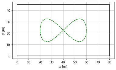
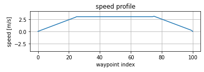
Figure 7: The plot shows the target trajectory given by the parametric curve $\gamma=(\gamma_{1},\gamma_{2}):[-\pi,\pi]\to\mathbb{R}^{2}$, where $\gamma_{1}(t)=40+20\cos(t)$, $\gamma_{2}(t)=22.5+20\sin(t)\cos(t)$, and the target speed profile.

In the driving simulation, the parameter values

$$a_{max}=5,\vartheta_{max}=\pi/6,\rho_{1}=1,\rho_{2}=5,m=15,n=17.$$

were used. In the reference segment selection procedure a lookahead distance of $3$ meters was used to obtain the current reference segment and the corresponding cross track error. For details we refer again to [7]. Regarding the reward function we used the following values

$\alpha_{1}$	$\alpha_{2}$	$\alpha_{3}$	$\alpha_{4}$	$\beta_{1}$	$\beta_{2}$	$\lambda$	$r_{crash}$
$1$	$1$	$1$	$1.5$	$0.25$	$0.25$	$0.75$	$-250$

The PPO from the Stable Baselines package (version 2.10.0) is applied using the default parameter settings.

VI-A Pure path following

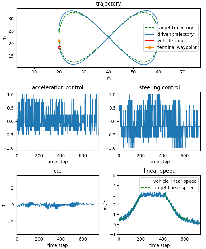
Figure 8: The plot shows the trajectory driven by the robot in the Python training simulation in an obstacle-free scenario. The plot shows moreover the controls applied over time, the cross track errors at each time point and the linear speed profile of the vehicle.

Figure 8 shows path following performance of the decision-making function in an obstacle-free environment. We observe that the driven trajectory almost matches the target trajectories. The deviations in the curved parts of the target trajectory can be attributed to the waypoint selection procedure and the controller’s effort to minimise the cross track error. Moreover we note, that the target velocity profile is reached very precisely. Summing up, we expect a small value of $\kappa_{2}$ and a value close to $1$ of $\kappa_{reach}$. Considering $50$ randomly generated points on the target trajectory and a positional tolerance of $1$ meters, we obtain

$$\kappa_{2}=0.04,~{}~{}~{}~{}~{}\kappa_{reach}=0.94.$$

VI-B Reactive path following

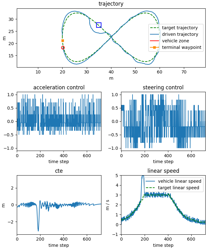
Figure 9: The figure shows the target trajectory and as well the trajectory driven by the vehicle.

To illustrate the ability of the decision-making function to detect and evade an obstacle along the target trajectory, we consider a scenario with one obstacle placed on the target trajectory. The resulting trajectory of the vehicle is given in Figure 9. In regard of the KPIs we obtain the following values

$$\kappa_{2}=0.36,~{}~{}~{}~{}~{}\kappa_{reach}=0.14$$

$$\kappa_{dist}=0.75,~{}~{}~{}~{}~{}\kappa_{danger}=0.02$$

We point out that, caused by the evasion maneuver, the value of $\kappa_{2}$ increases and the waypoint reach rate $\kappa_{danger}$ drops rather strongly. The latter is a consequence of the necessary wide swerving to avoid a collision.

VII Discussion and outlook

VII-A Discussion

We were able to define and train by means of a state of the art RL algorithm a decision-making function solving the reactive path tracking problem as introduced in Section III. For the performance and safety assessment of the controller KPIs were considered. According to these KPIs decent results could be obtained. This is confirmed by the plots depicted in Figure 8 and Figure 9. Even though the target trajectory could be tracked in an sufficient manner, by means of adjustments of the reward function a smoother driving behaviour could be obtained.

To obtain a more valid and more reliable statement in regard of the safety performance of the decision-making function, further KPIs may be studied. Additionally, unit tests for the examination of the driving behaviours in selected (critical) scenarios could be considered. In order to complete picture the above validation and safety assessment procedure has to be applied to a larger set of different scenarios. Only then possible weaknesses of the approach can be identified. Based on these results, conclusions can be drawn about the quality and the completeness of the set of scenarios considered in the training process. In order to achieve a balanced and robust result, it is important to use samples from an uniform distribution over the whole input space of the ANN. This can be achieved by considering a wide variety of training scenarios.

VII-B Outlook

At the time of publication of this paper, the integration of the decision-making function into the SPIDER software stack had not yet been completed. Results from the tests carried out in Gazebo and in real-world scenarios could therefore not be considered. The publication will be supplemented in this respect during the remainder of the FRACTAL project.

VIII Acknowledgments

This project has received funding from the ECSEL Joint Undertaking (JU) under grant agreement No 877056. The JU receives support from the European Union’s Horizon 2020 research and innovation programme and Spain, Italy, Austria, Germany, Finland, Switzerland. In Austria the project was also funded by the program ”IKT der Zukunft” of the Austrian Federal Ministry for Climate Action (BMK). The publication was written at Virtual Vehicle Research GmbH in Graz and partially funded within the COMET K2 Competence Centers for Excellent Technologies from the Austrian Federal Ministry for Climate Action (BMK), the Austrian Federal Ministry for Digital and Economic Affairs (BMDW), the Province of Styria (Dept. 12) and the Styrian Business Promotion Agency (SFG). The Austrian Research Promotion Agency (FFG) has been authorised for the programme management.

References

- [1] Sergi Alcaide, Guillem Cabo, Francisco Bas, Pedro Benedicte, Francisco Fuentes, Feng Chang, Ilham Lasfar, Ramon Canal, and Jaume Abella. Safex: Open source hardware and software components for safety-critical systems. In 2022 Forum on Specification & Design Languages (FDL), pages 1–4, 2022.
- [2] Khaled Alomari, Ricardo Carrillo Mendoza, Daniel Goehring, and Raúl Rojas. Path following with deep reinforcement learning for autonomous cars. In ROBOVIS, pages 173–181, 2021.
- [3] Junjie Bai, Fang Lu, Ke Zhang, et al. ONNX: Open Neural Network Exchange. https://github.com/onnx/onnx, 2019.
- [4] Michele Cancilla, Laura Canalini, Federico Bolelli, Stefano Allegretti, Salvador Carrión, Roberto Paredes, Jon A. Gómez, Simone Leo, Marco Enrico Piras, Luca Pireddu, Asaf Badouh, Santiago Marco-Sola, Lluc Alvarez, Miquel Moreto, and Costantino Grana. The deephealth toolkit: A unified framework to boost biomedical applications. In 2020 25th International Conference on Pattern Recognition (ICPR), pages 9881–9888, 2021.
- [5] Xiuquan Cheng, Shaobo Zhang, Sizhu Cheng, Qinxiang Xia, and Junhao Zhang. Path-following and obstacle avoidance control of nonholonomic wheeled mobile robot based on deep reinforcement learning. Applied Sciences, 12(14):6874, 2022.
- [6] Salvador Dominguez, Alan Ali, Gaëtan Garcia, and Philippe Martinet. Comparison of lateral controllers for autonomous vehicle: Experimental results. In 2016 IEEE 19th International Conference on Intelligent Transportation Systems (ITSC), pages 1418–1423. IEEE, 2016.
- [7] Guillaume JJ Ducard. Fault-tolerant flight control and guidance systems: Practical methods for small unmanned aerial vehicles. Springer Science & Business Media, 2009.
- [8] Andreas Folkers, Matthias Rick, and Christof Büskens. Controlling an autonomous vehicle with deep reinforcement learning. In 2019 IEEE Intelligent Vehicles Symposium (IV), pages 2025–2031. IEEE, 2019.
- [9] Rodrigo Gutiérrez, Elena López-Guillén, Luis M Bergasa, Rafael Barea, Óscar Pérez, Carlos Gómez-Huélamo, Felipe Arango, Javier Del Egido, and Joaquín López-Fernández. A waypoint tracking controller for autonomous road vehicles using ros framework. Sensors, 20(14):4062, 2020.
- [10] Imen Hassani, Imen Maalej, and Chokri Rekik. Robot path planning with avoiding obstacles in known environment using free segments and turning points algorithm. Mathematical Problems in Engineering, 2018, 2018.
- [11] Carles Hernàndez, Jose Flieh, Roberto Paredes, Charles-Alexis Lefebvre, Imanol Allende, Jaume Abella, David Trillin, Martin Matschnig, Bernhard Fischer, Konrad Schwarz, Jan Kiszka, Martin Rönnbäck, Johan Klockars, Nicholas McGuire, Franz Rammerstorfer, Christian Schwarzl, Franck Wartet, Dierk Lüdemann, and Mikel Labayen. Selene: Self-monitored dependable platform for high-performance safety-critical systems. In 2020 23rd Euromicro Conference on Digital System Design (DSD), pages 370–377, 2020.
- [12] Ashley Hill, Antonin Raffin, Maximilian Ernestus, Adam Gleave, Anssi Kanervisto, Rene Traore, Prafulla Dhariwal, Christopher Hesse, Oleg Klimov, Alex Nichol, Matthias Plappert, Alec Radford, John Schulman, Szymon Sidor, and Yuhuai Wu. Stable baselines. https://github.com/hill-a/stable-baselines, 2018.
- [13] Gabriel M Hoffmann, Claire J Tomlin, Michael Montemerlo, and Sebastian Thrun. Autonomous automobile trajectory tracking for off-road driving: Controller design, experimental validation and racing. In 2007 American control conference, pages 2296–2301. IEEE, 2007.
- [14] B Ravi Kiran, Ibrahim Sobh, Victor Talpaert, Patrick Mannion, Ahmad A Al Sallab, Senthil Yogamani, and Patrick Pérez. Deep reinforcement learning for autonomous driving: A survey. IEEE Transactions on Intelligent Transportation Systems, 2021.
- [15] Jens Kober, J Andrew Bagnell, and Jan Peters. Reinforcement learning in robotics: A survey. The International Journal of Robotics Research, 32(11):1238–1274, 2013.
- [16] Jason Kong, Mark Pfeiffer, Georg Schildbach, and Francesco Borrelli. Kinematic and dynamic vehicle models for autonomous driving control design. In 2015 IEEE intelligent vehicles symposium (IV), pages 1094–1099. IEEE, 2015.
- [17] Dimitri Leca, Viviane Cadenat, and Thierry Sentenac. Sensor-based algorithm for collision-free avoidance of mobile robots in complex dynamic environments. In 2019 European Conference on Mobile Robots (ECMR), pages 1–6. IEEE, 2019.
- [18] Aizea Lojo, Leire Rubio, Jesus Miguel Ruano, Tania Di Mascio, Luigi Pomante, Enrico Ferrari, Ignacio Garcìa Vega, Frank K. Gürkaynak, Mikel Labayen Esnaola, Vanessa Orani, and Jaume Abella. The ecsel fractal project: A cognitive fractal and secure edge based on a unique open-safe-reliable-low power hardware platform. In 2020 23rd Euromicro Conference on Digital System Design (DSD), pages 393–400, 2020.
- [19] Eivind Meyer, Haakon Robinson, Adil Rasheed, and Omer San. Taming an autonomous surface vehicle for path following and collision avoidance using deep reinforcement learning. IEEE Access, 8:41466–41481, 2020.
- [20] Hector Perez-Leon, Jose Joaquin Acevedo, Jose A Millan-Romera, Alejandro Castillejo-Calle, Ivan Maza, and Anibal Ollero. An aerial robot path follower based on the ‘carrot chasing’algorithm. In Iberian Robotics conference, pages 37–47. Springer, 2019.
- [21] Philip Polack, Florent Altché, Brigitte d’Andréa Novel, and Arnaud de La Fortelle. The kinematic bicycle model: A consistent model for planning feasible trajectories for autonomous vehicles? In 2017 IEEE intelligent vehicles symposium (IV), pages 812–818. IEEE, 2017.
- [22] Seyyed Mohammad Hosseini Rostami, Arun Kumar Sangaiah, Jin Wang, and Xiaozhu Liu. Obstacle avoidance of mobile robots using modified artificial potential field algorithm. EURASIP Journal on Wireless Communications and Networking, 2019(1):1–19, 2019.
- [23] Moveh Samuel, Mohamed Hussein, and Maziah Binti Mohamad. A review of some pure-pursuit based path tracking techniques for control of autonomous vehicle. International Journal of Computer Applications, 135(1):35–38, 2016.
- [24] John Schulman, Filip Wolski, Prafulla Dhariwal, Alec Radford, and Oleg Klimov. Proximal policy optimization algorithms. arXiv preprint arXiv:1707.06347, 2017.
- [25] Emrah Akin Sisbot, Luis F Marin, and Rachid Alami. Spatial reasoning for human robot interaction. In 2007 IEEE/RSJ International Conference on Intelligent Robots and Systems, pages 2281–2287. IEEE, 2007.
- [26] Jorge Sola and Joaquin Sevilla. Importance of input data normalization for the application of neural networks to complex industrial problems. IEEE Transactions on nuclear science, 44(3):1464–1468, 1997.
- [27] Richard S Sutton and Andrew G Barto. Reinforcement learning: An introduction. MIT press, 2018.
- [28] Marc Toussaint. Robot trajectory optimization using approximate inference. In Proceedings of the 26th annual international conference on machine learning, pages 1049–1056, 2009.
- [29] Johannes Ultsch, Jonas Mirwald, Jonathan Brembeck, and Ricardo de Castro. Reinforcement learning-based path following control for a vehicle with variable delay in the drivetrain. In 2020 IEEE Intelligent Vehicles Symposium (IV), pages 532–539. IEEE, 2020.
- [30] Stavros G Vougioukas. Reactive trajectory tracking for mobile robots based on non linear model predictive control. In Proceedings 2007 IEEE International Conference on Robotics and Automation, pages 3074–3079. IEEE, 2007.
- [31] Martin S Wiig, Kristin Y Pettersen, and Thomas R Krogstad. A 3d reactive collision avoidance algorithm for nonholonomic vehicles. In 2018 IEEE Conference on Control Technology and Applications (CCTA), pages 67–74. IEEE, 2018.