This is some thing

Dynamics at the edge for independent diffusing particles

Abstract

We study the dynamics of the outliers for a large number of independent Brownian particles in one dimension. We derive the multi-time joint distribution of the position of the rightmost particle, by two different methods. We obtain the two time joint distribution of the maximum and second maximum positions, and study the counting statistics at the edge. Finally we derive the multi-time joint distribution of the running maximum, as well as the joint distribution of the arrival time of the first particle at several space points.

1   Introduction

The maximum of a large number $N\gg 1$ of identical independent Brownian motions, started from the origin in one dimension, properly rescaled and centered, is distributed according to the Gumbel distribution, one of the three classes of extreme value statistics [1, 2, 3, 4]. Recently, there has been renewed interest in the statistics of the particles at the edge of a cloud of Brownian particles diffusing in a common space-time dependent random environment [5, 6, 7, 8, 9, 10, 11, 12, 13]. For a large number of particles, it was shown that on top of the Gumbel fluctuations, there is a random, environment-dependent shift in the position of the rightmost particle. Furthermore, the statistics of this shift was found to be related to those of some solutions of the Kardar-Parisi-Zhang equation. Tracer diffusion experiments, involving colloid or photons, are presently aiming to test that prediction [14].

This prediction is about the position of the maximum at a given time, a one-time observable. It would be interesting to extend it to multi-time observables. With this longstanding aim in mind, one can start by asking about a much simpler problem, namely multi-time observables for identical independent Brownian motions, in the absence of a background environment. That should be useful, e.g. as a benchmark in the analysis of such experiments.

In the present paper we study the dynamics of the outliers for a large number of independent Brownian particles on the line, all starting at the origin. We derive the multi-time joint distribution of the position of the rightmost particle, i.e. of the maximum of all the particle positions, by two elementary methods, which lead to different, though equivalent, formulae. The first method is standard for extreme value statistics, the second uses the diffusion equation. We obtain explicit formula for the cumulants of the fluctuations of the maximum at different times. We then extend these results to the multi-time joint distribution of the maximum and of the second maximum particle positions. In parallel, we obtain some predictions about the counting statistics at the edge of the cloud, which describes the outliers. Next, we study some continuum time observables of the rescaled maximum process. We obtain the probability that it remains below some level during some time interval. We study the running maximum, that is the maximum over all the particles and up to some fixed time, and obtain its multi-time joint distribution. Finally, we obtain the joint distribution of the arrival times of the first particle (i.e. the first detection times) at different locations in space, and the distribution of the time delays between these detection events.

It must be noted that this class of problems is related to the so-called multivariate extreme value theory and max-stable processes, which has a long history, starting with the Brown-Resnick process [15, 16] and the Husler-Reiss (HR) distributions [17, 18]. Since these seminal papers there were a number of extensions [19, 20, 21, 22, 23, 24, 25, 26], though apparently mainly in the fields of probability and statistics. Our modest aim here is to instead study the problem with simple heuristic methods of statistical physics. In the course of our work we will encounter some known objects, such as the HR distributions, in sometimes different forms, but we will also study more general outlier properties, counting statistics, the running maximum problem, and arrival time statistics. One must also note an independent work in preparation on these topics [27], following upon the recent work [28] which studies counting statistics for stochastic processes with an extended initial condition.

The outline of the paper is as follows. In Section 2 we focus on one-time observables (maximum, order and counting statistics of outliers) and recall the standard results obtained for these quantities from extreme value statistics of i.i.d random variables. In Section 3 (and Appendix A) we give a first derivation of the multi-time distribution of the maximum. In Section 4 we give more explicit formula for some marginals, moments and two and three time correlations of the maximum. The relevant calculations are detailed in Appendices B and C. In Section 5 we present a second derivation of the multi-time distribution of the maximum based on the heat equation. It naturally allows to obtain these distributions recursively. In Section 6 we study some multi-time properties of the outliers, e.g. we obtain the multi-time joint distribution for the maximum and second maximum, either directly, in Appendix D, or by studying counting statistics near the edge of the cloud. In Appendix E it is indicated how to extend these results to any rank at number of times. Finally, in Section 7 and Appendix F we study continuum time observables of the rescaled maximum process, as well as the multi-time statistics of the running maximum and of the arrival times of the first particle.

2   Outliers at a given time

Let us start by recalling standard results of extreme value statistics [1, 2, 3, 4], applied to one time observables for diffusing particles.

2.1   Maximum at a given time

Let us consider a particle whose position $x(t)$ evolves according to a random process. Let us denote $p_{t}(x)$ the one time probability distribution function (PDF) of the position at time $t$. The example on which we will focus will be a Brownian particle, $x(t)=\sqrt{2D}B(t)$, started at $x=0$ at time $t=0$. In that case $p_{t}(x)=\frac{1}{\sqrt{4Dt}}e^{-x^{2}/(4Dt)}$ is the standard diffusion kernel. Below we set $D=1$ since any value of $D$ can be restored by a rescaling of time.

Let us now consider $N$ identical copies of that particle evolving independently. In our canonical example all the Brownian particles have the same diffusion coefficient and all start from $x=0$ at time $t=0$. One now defines the position of the rightmost particle, i.e. the maximum $X(t)=\max_{i=1,\dots,N}x_{i}(t)$. We are interested in the case where $N$ is large. By definition the cumulative distribution function (CDF) of the maximum is given by

$$Q(X)={\rm Prob}(X(t)<X)=P_{<,t}(X)^{N}=e^{N\log(1-P_{>,t}(X))}\underset{N\gg 1}{\simeq}e^{-NP_{>,t}(X)}$$ (1)

where we denote $P_{>,t}(X)=\int_{X}^{+\infty}dxp_{t}(x)$ and $P_{<,t}(X)=\int_{-\infty}^{X}dxp_{t}(x)$. As is well known, the standard diffusion falls in the Gumbel extremal class. For any process in that class one can simply perform the change of variable from $X$ to $z$ defined by

$$NP_{>,t}(X)=e^{-z}$$ (2)

In the case of diffusion it gives $\frac{N\sqrt{t}}{\sqrt{2\pi}X}e^{-X^{2}/(2t)}=e^{-z}$ leading to

$$X\simeq\sqrt{2t}(\sqrt{\log N}+\frac{z+c_{N}}{2\sqrt{\log N}})\quad,\quad c_{N}=-\frac{1}{2}\log(4\pi\log N)$$ (3)

In this new variable the CDF is simply the Gumbel distribution, $e^{-e^{-z}}$, i.e. one has

$$Q(X)={\rm Prob}(X(t)<X)\simeq e^{-e^{-z}}$$ (4)

Note that the change of variable (2) (hence also (3) to leading order) is such that one has exactly

$$Np_{t}(X)dX=e^{-z}dz$$ (5)

In the following we will often (abusively) also consider $z$ as the random variable defined by (3) with $X=X(t)$, i.e. as the rescaled position of the maximum.

2.2   Order statistics of outliers

It is well known how to extend this to the $k$ first particles [2, 3, 4]. Let us denote $X^{(j)}(t)$ the same set of particles, but ordered by their rank, i.e. $X^{(1)}(t)>X^{(2)}(t)>\dots>X^{(N)}(t)$, so that $X(t)=X^{(1)}(t)$ is the position of the maximum, $X^{(2)}(t)$ of the second maximum and so on.

The joint PDF of the $k$ first outliers is

$$N(N-1)\dots(N-k+1)p_{t}(X^{(1)})p_{t}(X^{(2)})\dots p_{t}(X^{(k)})\theta_{X^{(1)}>\dots>X^{(k)}}P_{<,t}(X^{(k)})^{N-k}dX^{(1)}\dots dX^{(k)}$$ (6)

For large $N$ it becomes

$$\simeq\left(\prod_{j=1}^{k}(Np_{t}(X^{(j)})dX^{(j)})\right)\theta_{X^{(1)}>\dots>X^{(k)}}e^{-NP_{>,t}(X^{(k)})}$$ (7)

Thus the same change of variable

$$NP_{>,t}(X^{(j)})=e^{-z^{(j)}}$$ (8)

which in the case of diffusion reads

$$X^{(j)}\simeq\sqrt{2t}(\sqrt{\log N}+\frac{z^{(j)}+c_{N}}{2\sqrt{\log N}})$$ (9)

allows to put the large $N$ asymptotic joint PDF of the position of the $k$ first particles in the well known form

$$q(z^{(1)},\dots,z^{(k)})=\theta_{z^{(1)}>z^{(2)}>\dots>z^{(k)}}\,e^{-z^{(1)}-z^{(2)}-\dots-z^{(k)}}e^{-e^{-z^{(k)}}}$$ (10)

or equivalently as

$$q(z^{(1)},\dots,z^{(k)})=\theta_{z^{(1)}>z^{(2)}>\dots>z^{(k)}}\,\prod_{\ell=1}^{k-1}\ell e^{-\ell(z^{(\ell)}-z^{(\ell+1)})}\times\frac{1}{(k-1)!}e^{-kz^{(k)}-e^{-z^{(k)}}}\;.$$ (11)

Hence to generate the $k$ largest points, one first chooses $z_{k}$ and then the successive gaps as independent exponentially distributed variables, with distinct parameters.

2.3   Counting statistics of outliers

Another standard way to characterize the outliers is the counting statistics. Let us define $n_{X}$ as the number of particles at a given time $t$ with $x_{i}(t)>X$. Since the particles are identical and independent the probability that $n_{X}=n$ follows the binomial distribution

$$P_{X}(n)=\frac{N!}{n!(N-n)!}P_{<,t}(X)^{N-n}P_{>,t}(X)^{n}$$ (12)

In the edge regime for large $X$, i.e. for $NP_{>,t}(X)=O(1)$ this becomes a Poisson distribution

$$P_{X}(n)\simeq\frac{1}{n!}(NP_{>,t}(X))^{n}e^{-NP_{>,t}(X)}=\frac{1}{n!}e^{-nz}e^{-e^{-z}}$$ (13)

where in the last equality we have used the change of variable (2). In the case of independent Brownian motions, all starting from the origin, the variables $X$ and $z$ are related through (3). From it one recovers the Gumbel CDF of the maximum

$$P_{X}(n=0)={\rm Prob}(X(t)<X)\simeq e^{-e^{-z}}$$ (14)

Note that the other probabilities have also some interpretations in terms of order statistics, i.e. $P_{X}(1)={\rm Prob}(X(t)>X,X^{(2)}(t)<X)$, where $X(t)=X^{(1)}(t)$ and $X^{(2)}(t)$ are the maximum and second maximum respectively, and so on. Furthermore one sees that $X^{(k)}<X$ is equivalent to $n_{X}\in\{0,1,\dots,k-1\}$, hence

$${\rm Prob}(X^{(k)}<X)\simeq(\sum_{n=0}^{k-1}\frac{1}{n!}e^{-nz})e^{-e^{-z}}$$ (15)

One can check that taking $\partial_{z}$ of the r.h.s. one recovers the PDF of $z=z^{(k)}$, i.e. $q(z^{(k)})=\frac{1}{(k-1)!}e^{-kz^{(k)}-e^{-z^{(k)}}}$.

How does one recover the joint PDF of $X(t)$ and $X^{(2)}(t)$ ? For that one needs the joint PDF of $n_{X_{1}}$ and $n_{X_{2}}$ with $X_{1}>X_{2}$ where we recall that $n_{X}$ the number of particles with $x_{i}(t)>X$. To obtain it we split the line into three disjoint intervals (a) $x>X_{1}$, (b) $X_{2}<x<X_{1}$ and (c) $x<X_{2}$ and write the product of sums of probabilities of these events

$$1=(P(x>X_{1})+P(X_{2}<x<X_{1})+P(x<X_{2}))^{N}$$ (16)

Here for convenience we adopt the shorthand notations, e.g. $P(X_{2}<x<X_{1})=\int_{X_{2}}^{X_{1}}dxp_{t}(x)$ and so on. Expanding (16), we see that the probability $P_{X_{1},X_{2}}(n_{a},n_{b},n_{c})$ that there are $n_{a},n_{b},n_{c}$ particles in each of these intervals, is given by the multinomial distribution

$$P_{X_{1},X_{2}}(n_{a},n_{b},n_{c})=\frac{N!}{n_{a}!n_{b}!n_{c}!}\delta_{N,n_{a}+n_{b}+n_{c}}P(x>X_{1})^{n_{a}}P(X_{2}<x<X_{1})^{n_{b}}P(x<X_{2})^{n_{c}}$$ (17)

In the large $N$ limit and choosing $X_{1}$ and $X_{2}$ near the edge so that typically $n_{b},n_{c}=O(1)$ while $n_{a}\simeq N$, one obtains by similar manipulations as above that the probability of $n_{a},n_{b}$ is a multiple independent Poisson distribution

$$P_{X_{1},X_{2}}(n_{a},n_{b})\simeq\frac{1}{n_{a}!n_{b}!}(e^{-z_{2}}-e^{-z_{1}})^{n_{b}}e^{-n_{a}z_{1}}e^{-e^{-z_{2}}}$$ (18)

which is correctly normalized to unity. This form applies to any problem of i.i.d random variables in the Gumbel class through the change of variable (2), and for our purpose here $X_{1}$ and $z_{1}$ are related through (3) and so are $X_{2}$ and $z_{2}$.

Several observables can be obtained from (18). For instance the joint PDF of $X(t)$ and $X^{(2)}(t)$ can be retrieved from taking $-\partial_{X_{1}}\partial_{X_{2}}$ of the following ”CDF”

$${\rm Prob}(X^{(2)}(t)<X_{2},X^{(1)}(t)>X_{1})=P_{X_{1},X_{2}}(n_{a}=1,n_{b}=0)\simeq e^{-z_{1}}e^{-e^{-z_{2}}}$$ (19)

and one can check that it is indeed equal to $\int_{y_{1}>z_{1}}\int_{y_{2}<z_{2}}e^{-y_{1}-y_{2}}e^{-e^{-y_{2}}}$.

Another interesting observable is the joint PDF of the couple $(n_{X_{1}},n_{X_{2}})$. Since the intervals $[X_{2},+\infty[$ and $[X_{1},+\infty[$ overlap, the two variables are correlated. One can write $(n_{X_{1}},n_{X_{2}})=(n_{a},n_{a}+n_{b})$, where $n_{a}$, $n_{b}$ are independent Poisson variables. Hence

$${\rm Prob}(n_{X_{1}}=n_{1},n_{X_{2}}=n_{2})=\theta_{n_{2}\geq n_{1}}\frac{\lambda_{a}^{n_{1}}}{n_{1}!}\frac{\lambda_{b}^{n_{2}-n_{1}}}{(n_{2}-n_{1})!}e^{-\lambda_{a}-\lambda_{b}}$$ (20)

with $\lambda_{a}=e^{-z_{1}}$ and $\lambda_{b}=e^{-z_{2}}-e^{-z_{1}}$ are the mean parameters of the distribution (18).

3   Multi-time joint CDF for the maximum: first method

Let us now consider the dynamics of the maximum $X(t)$. Its one time CDF is given by (3)-(4). What is the multi-time joint CDF of $X(t_{1}),X(t_{2}),\dots X(t_{n})$ ?

Let us first determine on what time scale these variables remain correlated. The first simple consideration is as follows. As recalled in Section 2.2, at any fixed time the gap between the maximum $z^{(1)}$ and the second maximum $z^{(2)}$ (in the variable $z$ seen as random variables) is $z^{(1)}-z^{(2)}=O(1)$. Hence at a given time $t=t_{1}$, from (9), the first gap is $X(t)-X^{(2)}(t)=O(\sqrt{t_{1}/\log N})$. These two rightmost particles undergo diffusion, hence it takes typically a time $t_{2}-t_{1}\sim(X(t)-X^{(2)}(t))^{2}\sim t_{1}/\log N$ for them to meet. This gives the scale of the time difference at which the order of the first few particles at the edge reshuffles, and correlations start decaying. For time differences much larger $t_{2}-t_{1}\gg t_{1}/\log N$ we expect that $X(t_{1})$ and $X(t_{2})$ become uncorrelated, each described, under the appropriate scaling, by Gumbel distributions.

Let us give the result for the joint CDF ${\rm Prob}(X(t_{1})<X_{1},\dots,X(t_{n})<X_{n})$. In view of the previous paragraph we define the dimensionless rescaled time differences $\tau_{i}$ as

$$t_{j}=t_{1}(1+\frac{\tau_{j,1}}{\log N})$$ (21)

with the notation $\tau_{i,j}=\tau_{i}-\tau_{j}$ and $\tau_{1}=0$. As above one performs the change of variable

$$X_{j}=\sqrt{2t_{j}}\sqrt{\log N}(1+\frac{z_{j}+c_{N}}{2\log N})\simeq\sqrt{2t_{1}}\sqrt{\log N}(1+\frac{z_{j}+\tau_{j,1}+c_{N}}{2\log N})$$ (22)

Then, at large $N$ we obtain (by similar manipulations as in the previous section, see Appendix A) that the joint CDF takes the form

$${\rm Prob}(X(t_{1})<X_{1},\dots,X(t_{n})<X_{n})\simeq\exp\left(-\Phi(z_{1},\dots,z_{n};\tau_{2,1},\dots,\tau_{n,n-1})\right)$$ (23)

$$\Phi(z_{1},\dots,z_{n};\tau_{2,1},\dots,\tau_{n,n-1})=\int_{y_{1},\dots,y_{n}}(1-\prod_{i=1}^{n}\theta_{y_{i}<z_{i}})e^{-y_{1}}G(y_{2,1},\tau_{2,1})\dots G(y_{n,n-1},\tau_{n,n-1})$$ (24)

where here and below we often use the notations $y_{i,j}=y_{i}-y_{j}$ and the shorthand $\int_{y}=\int dy=\int_{-\infty}^{+\infty}dy$ as well as $\theta_{y<z}=\theta_{z>y}=\theta(z-y)$ where $\theta(x)$ is the Heaviside function, and

$$G(y,\tau)=\frac{1}{\sqrt{4\pi\tau}}e^{-\frac{(y+\tau)^{2}}{4\tau}}$$ (25)

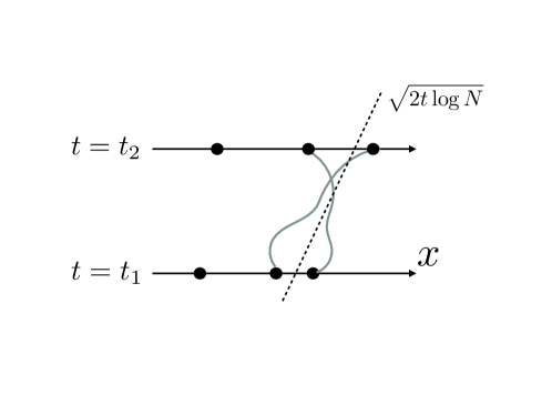
is simply the free diffusion kernel, however with a negative unit drift (and with $D=2$). This drift originates from the fact that the position of the maximum increases with time, as can be seen e.g. in (22). Hence the front of the cloud of particles moves to the right and with respect to this front the diffusion of a single particle, which is symmetric, has a negative drift. This is why, as we will see below, the correlations decay exponentially at large time: after a scaled time difference $\tau=O(1)$ the cloud of particles overtakes the particle which was the rightmost at time $t_{1}$. This is illustrated in Fig. 1. Finally, the factor $e^{-y_{1}}$ reminds that the Gumbel distribution is a (non-normalizable) stationary distribution of the rescaled maximum process in the $z$ variable (see below).

Although exact, the above formula is delicate. Indeed each of the two terms in $(1-\prod_{i=1}^{n}\theta_{y_{i}<z_{i}})$ is a divergent integral (for $y_{j}\to y_{j}+y$ with $y\to-\infty$), and only the combination is finite and the terms cannot be separated.

Let us give an equivalent formula for $n=2$. One recombine as

$$1-\theta_{y_{1}<z_{1}}\theta_{y_{2}<z_{2}}=1-(1-\theta_{z_{1}<y_{1}})(1-\theta_{z_{2}<y_{2}})=\theta_{z_{1}<y_{1}}+\theta_{z_{2}<y_{2}}-\theta_{z_{1}<y_{1}}\theta_{z_{2}<y_{2}}$$ (26)

We use the important property that $e^{-z_{1}}dz_{1}$ is a (non-normalizable) stationary measure of the free diffusion with a negative unit drift, i.e. it satisfies

$$\int dz_{1}e^{-z_{1}}G(z_{2,1},\tau_{2,1})=e^{-z_{2}}$$ (27)

for any real $z_{1},z_{2}$ and $\tau_{2,1}>0$, where we here and below use the notation $z_{2,1}=z_{2}-z_{1}$. The other important property is the normalization condition

$$\int dy\,G(y,\tau)=1$$ (28)

Using these two properties, inserting (26) into (24) one finds

$$\Phi(z_{1},z_{2};\tau_{2,1})=e^{-z_{1}}+e^{-z_{2}}-\int_{z_{1}<y_{1},z_{2}<y_{2}}e^{-y_{1}}G(y_{2,1},\tau_{2,1})$$ (29)

This function admits an explicit expression in terms of error functions, it is given below in (39) and (40) and in (238) in the Appendix.

Let us now generalize this formula to arbitrary $n$. Starting from $n=3$ one must also use a third property, the convolution identity

$$\int dy\,G(z,y,\tau^{\prime})G(y,x,\tau)=G(z,x,\tau+\tau^{\prime})$$ (30)

It is then easy to see, using these three properties, that one has

$$\Phi(z_{1},z_{2};\tau_{2,1})=e^{-z_{1}}+e^{-z_{2}}-g(z_{1},z_{2};\tau_{2,1})$$ (31)

$$\Phi(z_{1},z_{2},z_{3};\tau_{2,1},\tau_{3,2})=e^{-z_{1}}+e^{-z_{2}}+e^{-z_{3}}$$ (32)

$$-g(z_{1},z_{2};\tau_{2,1})-g(z_{2},z_{3};\tau_{3,2})-g(z_{1},z_{3};\tau_{31})+g_{3}(z_{1},z_{2},z_{3};\tau_{2,1},\tau_{3,2})$$

and so on, where we have defined

$$g(z_{1},z_{2};\tau_{2,1})=\int_{z_{1}<y_{1},z_{2}<y_{2}}e^{-y_{1}}G(y_{2,1},\tau_{2,1})=e^{-z_{1}}\int_{0<y_{1},0<y_{2}}e^{-y_{1}}G(y_{2,1}+z_{2,1},\tau_{2,1})$$ (33)

$$g_{3}(z_{1},z_{2},z_{3};\tau_{2,1},\tau_{3,2})=\int_{z_{1}<y_{1},z_{2}<y_{2},z_{3}<y_{3}}e^{-y_{1}}G(y_{2,1},\tau_{2,1})G(y_{3,2},\tau_{3,2})$$ (34)

$$=e^{-z_{1}}\int_{0<y_{1},0<y_{2},0<y_{3}}e^{-y_{1}}G(y_{2,1}+z_{2,1},\tau_{2,1})G(y_{3,2}+z_{3,2},\tau_{3,2})$$ (35)

and so on, with more generally, for $a_{1}<\dots<a_{k}$, $k\geq 1$

$$g_{k}(z_{a_{1}},\dots,z_{a_{k}};\tau_{a_{2},a_{1}},\dots,\tau_{a_{k},a_{k-1}})=\int_{z_{a_{1}}<y_{a_{1}},\dots,z_{a_{k}}<y_{a_{k}}}e^{-y_{a_{1}}}G(y_{a_{2},a_{1}},\tau_{a_{2},a_{1}})\dots G(y_{a_{k},a_{k-1}},\tau_{a_{k},a_{k-1}})$$ (36)

with $g_{2}=g$ and $g_{1}(z)=e^{-z}$. It is easy to see from the above properties (30) and (27) that if any argument $z_{a_{j}}$ for some $j$ in $g_{k}$ is set to $z_{a_{j}}=-\infty$ then $g_{k}\to g_{k-1}$ and $z_{a_{j}}$ and $\tau_{j}$ are dropped from the list of arguments. Also, any $g_{k}$ obviously vanishes when any $z_{a_{j}}$ for some $j$ argument is taken to $+\infty$.

One can see on (33) and (35) that one can always factor out the term $e^{-z_{1}}$, the rest being only function of differences of $z_{j}$’s. This important factorization property is true for any $n$, i.e. one can always write

$$\Phi(z_{1},\dots,z_{n};\tau_{2,1},\dots,\tau_{n,n-1})=e^{-z_{1}}\phi_{\tau_{2,1},\dots,\tau_{n,n-1}}(z_{2,1},\dots,z_{n,n-1})$$ (37)

The functions $\phi$ will be further studied below.

The above result provides explicit, although lengthy, expressions for the multi-time joint CDF of the maximum. As we will see below, using a second method based on the heat equation, the functions $\Phi$ can also be computed recursively with $n$. This leads to more compact expressions. Before explaining that, let us give some explicit results for marginals, cumulants and correlation functions for $n=2$ and $n=3$.

Figure 1: Schematic view of the positions of the three rightmost particles at two times, with $t_{2}-t_{1}=t_{1}(1+\frac{\tau}{\log N})$. The dotted line is the average position of the edge, which moves to the right with unit velocity in the scaled space-time variables $z,\tau$. The scaled maximum process is stationary in the frame moving with the edge. However the particle of maximal position at $t_{1}$ undergoes symmetric diffusion, and as $\tau$ increases is overtaken by the other particles in a time $\tau=O(1)$, leading to exponential decay of correlations.

4   Multi-time marginals, moments and correlations for the maximum

Let us analyze in more details the joint PDF obtained in the previous section. We will derive very explicit results for $n=2$, and give some general formula for $n=3$.

4.1   Two time correlations

Let us start with $n=2$.

4.1.1 Two time joint CDF

One recalls that at large $N$ with $t_{2}-t_{1}=t_{1}\frac{\tau_{2,1}}{\log N}$, with $\tau_{2,1}=\tau=O(1)$, the joint CDF for the position of the maximum takes the form

$${\rm Prob}(X(t_{1})<X_{1},X(t_{2})<X_{2})\simeq Q_{<,<}(z_{1},z_{2})=\exp\left(-\Phi(z_{1},z_{2};\tau)\right)$$ (38)

where we denote $Q_{<<}(z_{1},z_{2})$ the two-time CDF of the process in the variables $z_{j}$ (implicitely at times $t_{j}$), and $\Phi(z_{1},z_{2};\tau)$ was defined in (29). Through the change of variable $y_{j}\to y_{j}+z_{j}$ it can also be written as

$$\Phi(z_{1},z_{2};\tau)=e^{-z_{1}}\phi_{\tau}(z_{2,1})\quad,\quad\phi_{\tau}(z)=1+e^{-z}-\int_{y_{1}>0,y_{2}>0}e^{-y_{1}}G(y_{2,1}+z,\tau)$$ (39)

The integral can be computed, see Appendix B. This leads to the explicit form

$$\phi_{\tau}(z)=\frac{1}{2}\left(\text{erf}\left(\frac{\tau+z}{2\sqrt{\tau}}\right)+e^{-z}\text{erfc}\left(\frac{z-\tau}{2\sqrt{\tau}}\right)+1\right)$$ (40)

which obeys the important symmetry (see Appendix B)

$$\phi_{\tau}(z)e^{z}=\phi_{\tau}(-z)$$ (41)

This symmetry is equivalent to the fact that $\Phi(z_{1},z_{2};\tau)$ is symmetric in $z_{1},z_{2}$ as is visible on its explicit form (238) in the Appendix.

In summary the two time CDF of the maximum, in the rescaled variables, has the form

$$Q_{<<}(z_{1},z_{2})\simeq e^{-e^{-z_{1}}\phi_{\tau}(z_{2,1})}$$ (42)

where the function $\phi_{\tau}(z)$ is given in (40). As mentioned in the introduction, this distribution appeared before [17, 18] and is known as the bivariate HR distribution.

The function $\phi_{\tau}(z)$ has the following asymptotic behaviors for large argument

$$\phi_{\tau}(z)\simeq e^{-z}+\psi_{\tau}(z)\quad,\quad z\to-\infty$$ (43)

$$\phi_{\tau}(z)\simeq 1+\psi_{\tau}(z)\quad,\quad z\to+\infty$$ (44)

$$\psi_{\tau}(z)=e^{-\frac{(z+\tau)^{2}}{4\tau}}\frac{2\tau^{3/2}}{z^{2}\sqrt{\pi}}(1+\frac{\tau(\tau-6)}{z^{2}}+\frac{\tau^{2}(60+\tau(\tau-20)}{z^{4}}+O(z^{-6}))\quad,\quad|z|\to+\infty$$ (45)

Note that $\psi_{\tau}(-z)=e^{z}\psi_{\tau}(z)$. These asymptotics guarantee that one recovers the one time Gumbel CDF for $z_{1}\to+\infty$ or $z_{2}\to+\infty$, i.e. one has

$$Q_{<<}(z,+\infty)=Q_{<<}(+\infty,z)=e^{-e^{-z}}$$ (46)

In addition, at large $\tau$, since the free diffusion kernel with drift $G(y_{2,1}+z,\tau)\to 0$, one sees from (39) that

$$\phi_{\tau}(z)\simeq 1+e^{-z}\quad,\quad\Phi(z_{1},z_{2};\tau)\simeq e^{-z_{1}}+e^{-z_{2}}\quad,\quad\tau\to+\infty$$ (47)

which corresponds to two uncorrelated Gumbel variables.

4.1.2 Exponential moments of $z_{1}$ and $z_{2}$

Through (22) with $X_{j}=X(t_{j})$ one can (abusively) also think of $z_{1}$ and $z_{2}$ as random variables. Furthermore, from now on it is useful to consider $z_{1}$ and $z_{2,1}=z_{2}-z_{1}$ as the two random variables of interest.

A first result, see Appendix C, is an explicit integral expression for the joint moment generating function, which reads

$$\langle e^{-sz_{1}-bz_{2,1}}\rangle=\Gamma(1+s)\int dze^{-bz}\partial_{z}\left((1+\frac{\phi_{\tau}^{\prime}(z)}{\phi_{\tau}(z)})\frac{1}{\phi_{\tau}(z)^{s}}\right)$$ (48)

where here and below $\langle\dots\rangle$ denotes an expectation value. A simpler expression also exists for (48), see (257), but it is less convenient for the analysis of the moments. For $b=0$ the integral in (48) can be performed and the boundary term is $1$ at $z=+\infty$ and vanish at $z=-\infty$ (see Appendix C), recovering the generating function of the one-time Gumbel distribution

$$\langle e^{-sz_{1}}\rangle=\Gamma(1+s)$$ (49)

One also recovers the same result for $z_{2}$, by setting $b=s$, although the algebra is slightly more involved, see Appendix C.

4.1.3 PDF of $z_{2}-z_{1}$

It is possible to obtain explicitly the PDF of $X(t_{2})-X(t_{1})$ the distance over which the maximum has moved. One has from (22) that $X(t_{2})-X(t_{1})=\sqrt{\frac{t_{1}}{2\log N}}(\tau+z_{2,1})$, where we consider $z_{2,1}=z_{2}-z_{1}$ as a random variable. Its distribution is easily obtained. Indeed, (48) for $s=0$ implies the following expression for the generating function of the moments of $z_{2,1}$

$$\langle e^{-bz_{2,1}}\rangle=\int dze^{-bz}\partial_{z}(1+\frac{\phi_{\tau}^{\prime}(z)}{\phi_{\tau}(z)})$$ (50)

This, in turn, implies the following expressions for the PDF (denoted $P^{(2,1)}_{\tau}(z)$) and the CDF of the variable $z_{2,1}$

$$P^{(2,1)}_{\tau}(z)=\partial_{z}\frac{\phi_{\tau}^{\prime}(z)}{\phi_{\tau}(z)}=\partial_{z}^{2}\log\phi_{\tau}(z)\quad,\quad{\rm Prob}(z_{2,1}<z)=1+\partial_{z}\log\phi_{\tau}(z)$$ (51)

where $\phi_{\tau}(z)$ is given explicitly in (40). Thanks to the symmetry (41) we see that the PDF is an even function of $z$

$$P^{2,1}_{\tau}(-z)=P^{2,1}_{\tau}(z)$$ (52)

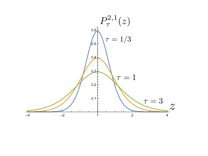
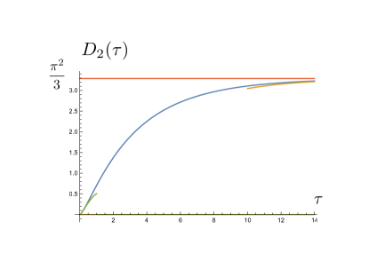
hence all odd moments of $z_{2,1}$ vanish. The PDF $P^{(2,1)}_{\tau}(z)$ is plotted in Fig. 2. Its behavior for large $|z|$ at fixed $\tau$ is

$$P^{2,1}_{\tau}(z)\simeq\frac{1}{\sqrt{4\pi\tau}}e^{-\frac{(|z|+\tau)^{2}}{4\tau}}(1+\frac{2\tau}{|z|}+\frac{2\tau^{2}}{z^{2}}+O(|z|^{-3})$$ (53)

hence for large argument is becomes equal to the free diffusion kernel with unit drift. Around $z=0$ it is analytic and behaves as

$$P^{2,1}_{\tau}(z)=\frac{1}{4}+\frac{e^{-\tau/4}}{\sqrt{\pi}\sqrt{\tau}\left(2\text{erf}\left(\frac{\sqrt{\tau}}{2}\right)+2\right)}-\frac{z^{2}}{16}\left(1+\frac{e^{-\tau/2}\left(\sqrt{\pi}e^{\tau/4}(5\tau+2)\left(\text{erf}\left(\frac{\sqrt{\tau}}{2}\right)+1\right)+6\sqrt{\tau}\right)}{\pi\tau^{3/2}\left(\text{erf}\left(\frac{\sqrt{\tau}}{2}\right)+1\right)^{2}}\right)+O(z^{4})$$ (54)

In the limit of large $\tau$ and fixed $z$ it converges to a finite limit

$$P^{2,1}_{\tau}(z)=\frac{1}{4\cosh^{2}(\frac{z}{2})}+O(e^{-\tau/4}\tau^{-1/2})$$ (55)

which is simply the PDF of the difference of two uncorrelated Gumbel variables, as it should. Indeed (55) implies

$$\lim_{\tau\to+\infty}\langle e^{-bz_{2,1}}\rangle=\frac{\pi b}{\sin(\pi b)}=\Gamma(1+b)\Gamma(1-b)$$ (56)

One can study how that limit is reached. One has, at large $\tau\gg 1$

$$\phi_{\tau}(z)=1+e^{-z}-e^{-\frac{(z+\tau)^{2}}{4\tau}}\chi_{\tau}(z)\quad,\quad\chi_{\tau}(z)=\frac{2}{\sqrt{\pi\tau}}(1-\frac{2}{\tau}+\frac{12+z^{2}}{\tau^{2}}+O(1/\tau^{3}))$$ (57)

Inserting into (51), expanding the logarithm to first order in $\chi_{\tau}(z)$, writing the exponential as $e^{-\frac{\tau}{4}-\frac{z}{2}}\times e^{-\frac{z^{2}}{4\tau}}$ and expanding the last factor in powers of $1/\tau$, one obtains the large $\tau$ expansion

$$P^{2,1}_{\tau}(z)=\frac{1}{4\cosh^{2}(\frac{z}{2})}+\frac{2e^{-\frac{\tau}{4}}}{\sqrt{\pi\tau}}\bigg{(}\frac{1}{16}\frac{3-\cosh(z)}{\cosh^{3}(\frac{z}{2})}+\frac{-3z^{2}+\left(z^{2}+16\right)\cosh(z)-8z\sinh(z)-16}{64\cosh^{3}(\frac{z}{2})\tau}+O(\tau^{-2})\bigg{)}$$ (58)

Figure 2: Left: marginal PDF of $z=z_{2,1}=z_{2}-z_{1}$, the scaled distance traveled by the maximum, with $X(t_{2})-X(t_{1})\simeq\sqrt{\frac{t_{1}}{2\log N}}(\tau+z)$. It is plotted for $\tau=1/3,1,3$. Right: its second moment $\langle z_{2,1}^{2}\rangle=A_{2}(\tau)$, plotted versus $\tau$. The first three terms in the small $\tau$ asymptotics (64), and the first two terms in the large $\tau$ asymptotics (62) are also plotted, together with the limiting value $\pi^{2}/3$. Recall that $\pi^{2}/3-A_{2}(\tau)$, i.e. the curve reflected versus $\pi^{2}/3$ describes the two-time covariance of the maximum, see Eq. (71).

4.1.4 Moments of $z_{2}-z_{1}$

We recall that the odd moments of $z_{2,1}=z_{2}-z_{1}$ vanish. One can further obtain formulae for the the even moments of $z_{2,1}$ by integration by part (boundary terms vanish), as, with $n\geq 1$

$$\langle z_{2,1}^{2n}\rangle=A_{2n}(\tau)=2\int_{0}^{+\infty}dzz^{2n}\partial_{z}^{2}\log\phi_{\tau}(z)=4n(2n-1)\int_{0}^{+\infty}dzz^{2n-2}\log\phi_{\tau}(z)$$ (59)

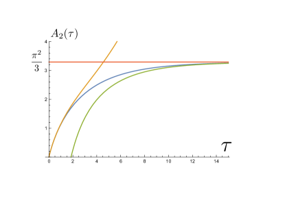
which are easy to evaluate numerically. The function $A_{2}(\tau)$ is plotted in Fig. 2. Using (56) one finds that at large time the moments tend to the moments of the difference of two uncorrelated Gumbel variables, namely

$$\lim_{\tau\to+\infty}\langle z_{2,1}^{2n}\rangle=A_{2n}(+\infty)=(-1)^{n+1}(2^{2n}-2)\pi^{2n}B_{2n}$$ (60)

where the $B_{k}$ are the Bernoulli numbers. The details asymptotics of $A_{2n}(\tau)$ at large $\tau$ is obtained as follows. From (57) one has

$$\log\phi_{\tau}(z)=\log(1+e^{-z})-e^{-\frac{(z+\tau)^{2}}{4\tau}}\frac{\chi_{\tau}(z)}{1+e^{-z}}+O(e^{-2\frac{(z+\tau)^{2}}{4\tau}})$$ (61)

and one performs similar manipulations as above. Using the last identity in (59), the integral on $z$ converges term by term in the expansion, leading to

$$\!\!\!\!\!\!A_{2}(\tau)=\frac{\pi^{2}}{3}-\frac{4\sqrt{\pi}e^{-\tau/4}}{\sqrt{\tau}}\left(1-\frac{8+\pi^{2}}{\tau}+\frac{12+\frac{3\pi^{2}}{2}+\frac{5\pi^{4}}{32}}{\tau^{2}}-\frac{120+15\pi^{2}+\frac{25\pi^{4}}{16}+\frac{61\pi^{6}}{384}}{\tau^{3}}+O(\tau^{-4})\right)$$ (62)

$$\!\!\!\!\!\!A_{4}(\tau)=\frac{7\pi^{4}}{15}-\frac{24\pi^{5/2}e^{-\tau/4}}{\sqrt{\tau}}\left(1-\frac{2+\frac{5\pi^{2}}{4}}{\tau}+\frac{12+\frac{15\pi^{2}}{2}+\frac{61\pi^{4}}{32}}{\tau^{2}}-\frac{120+75\pi^{2}+\frac{305\pi^{4}}{16}+\frac{1385\pi^{6}}{384}}{\tau^{3}}+O(\tau^{-4})\right)$$

At short time difference $\tau\ll 1$ the variable $z_{21}$ is of order $\sqrt{\tau}$. Defining the $O(1)$ random variable $w$ such that $z_{21}=w\sqrt{\tau}$ one finds that its PDF $p_{\tau}(w)$ admits a small $\tau$ expansion

$$p_{\tau}(w)=\frac{e^{-\frac{w^{2}}{4}}}{2\sqrt{\pi}}-\frac{\sqrt{\tau}\left(\sqrt{\pi}e^{-\frac{w^{2}}{4}}w\,\text{erf}\left(\frac{w}{2}\right)+\pi\left(\text{erf}\left(\frac{w}{2}\right)^{2}-1\right)+2e^{-\frac{w^{2}}{2}}\right)}{4\pi}+O\left(\tau\right)$$ (63)

So not surprisingly $z_{2,1}$ undergoes free diffusion at short time, but there are corrections as $\tau$ increases. The short time expansion of the lowest moments and cumulants, as well as of the kurtosis, reads

$$\langle z_{2,1}^{2}\rangle=\langle z_{2,1}^{2}\rangle^{c}=A_{2}(\tau)=2\tau-\frac{4}{3}\sqrt{\frac{2}{\pi}}\tau^{3/2}+0.217996\tau^{2}-0.0129398\tau^{5/2}+O(\tau^{3})$$ (64)

$$\langle z_{2,1}^{4}\rangle=A_{4}(\tau)=12\tau^{2}-\frac{72}{5}\sqrt{\frac{2}{\pi}}\tau^{5/2}+O(\tau^{3})~{},~{}\langle z_{2,1}^{4}\rangle^{c}=\frac{8}{5}\sqrt{\frac{2}{\pi}}\tau^{5/2}+O(\tau)~{},~{}{\rm Ku}=\frac{2}{5}\sqrt{\frac{2}{\pi}}\sqrt{\tau}+O(\tau)$$

$$\langle z_{2,1}^{6}\rangle=A_{6}(\tau)=120\tau^{3}-\frac{1380}{7}\sqrt{\frac{2}{\pi}}\tau^{7/2}+O(\tau^{4})$$

The small and large $\tau$ asymptotics are compared with the numerical calculation of $A_{2}(\tau)$ in Fig. 2.

4.1.5 Covariance of $X(t_{1})$ and $X(t_{2})$

Let us translate some of these results in the original variables. Let us recall the relations

$$X(t_{1})=X_{1}\simeq\sqrt{2t_{1}}(\sqrt{\log N}+\frac{z_{1}}{2\sqrt{\log N}})$$ (65)

$$X(t_{2})=X_{2}\simeq\sqrt{2t_{1}}(\sqrt{\log N}+\frac{\tau+z_{2}}{2\sqrt{\log N}})$$ (66)

Hence one has

$$X_{2}-X_{1}\simeq\sqrt{\frac{t_{1}}{2\log N}}(\tau+z_{2,1})\quad,\quad\tau=\frac{t_{2}-t_{1}}{t_{1}}\log N=O(1)$$ (67)

The results of the previous subsection thus imply for $\tau=O(1)$ and $p\geq 1$

$$\langle X_{2}-X_{1}\rangle\simeq\sqrt{\frac{t_{1}}{2\log N}}\,\tau,\quad,\quad\langle\left(X_{2}-X_{1}-\langle X_{2}-X_{1}\rangle\right)^{2p+1}\rangle=o((\frac{t_{1}}{2\log N})^{2p+1})$$ (68)

$${\rm Var}X_{1}={\rm Var}X_{2}\simeq\frac{t_{1}}{2\log N}\frac{\pi^{2}}{6}\quad,\quad{\rm Var}(X_{2}-X_{1})\simeq\frac{t_{1}}{2\log N}A_{2}(\tau)$$ (69)

$${\rm Cov}(X_{1},X_{2})=\frac{1}{2}({\rm Var}(X_{1})+{\rm Var}(X_{2})-{\rm Var}(X_{2}-X_{1}))$$ (70)

$$=\frac{t_{1}}{4\log N}(\frac{\pi^{2}}{3}-A_{2}(\tau))\quad,\quad A_{2}(\tau)=4\int_{0}^{+\infty}dz\log\phi_{\tau}(z)$$ (71)

where we have used the values for the first two moments of the Gumbel distribution, $\langle z_{1}^{2}\rangle=\langle z_{2}^{2}\rangle=\frac{\pi^{2}}{6}+\gamma_{E}^{2}$ and $\langle z_{1}\rangle=\langle z_{2}\rangle=\gamma_{E}$. The covariance is illustrated in Fig. 2. Using the asymptotics (62), we see that at large time difference $\tau\gg 1$ the covariance of the maximum at two different times decay as

$${\rm Cov}(X(t_{1}),X(t_{2}))\simeq\frac{t_{1}}{4\log N}\frac{4\sqrt{\pi}e^{-\tau/4}}{\sqrt{\tau}}$$ (72)

As discussed in the previous section, the large time decay is exponential since the particle which is the rightmost at time $t_{1}$ undergoes symmetric diffusion, while the front of the other particles advances, with an effective unit drift, on the time scales $\tau=O(1)$.

4.1.6 Correlations between $X(t_{1})$ and $X(t_{2})-X(t_{1})$

There are correlations between the variable $z_{1}$ and $z_{2,1}$. For instance from (48) one obtains

$$\langle z_{1}e^{-bz_{2,1}}\rangle-\langle z_{1}\rangle\langle e^{-bz_{2,1}}\rangle=-\int dze^{-bz}\partial_{z}\left((1+\frac{\phi_{\tau}^{\prime}(z)}{\phi_{\tau}(z)})\log\phi_{\tau}(z)\right)$$ (73)

The lowest cross moment is trivial

$$\langle z_{1}z_{2,1}\rangle=-\frac{1}{2}\langle z_{2,1}^{2}\rangle$$ (74)

The first non trivial cross cumulant is

$$\langle z_{1}z_{2,1}^{2}\rangle^{c}=\langle z_{1}z_{2,1}^{2}\rangle-\langle z_{1}\rangle\langle z_{2,1}^{2}\rangle=-\int dzz^{2}\partial_{z}\left((1+\frac{\phi_{\tau}^{\prime}(z)}{\phi_{\tau}(z)})\log\phi_{\tau}(z)\right)$$ (75)

which upon rescaling yields the corresponding cross cumulant for the maximum $X(t_{1})$ and its variation $X(t_{2})-X(t_{1})$.

4.1.7 Conditional probability of $z_{1}$ given $z_{2}-z_{1}$

It is also interesting to compute the PDF of $z_{1}$ conditioned on a given value of $z_{2,1}=z$, which turns out to have a simple form. One finds

$$q_{\tau}(z_{1}|z_{2,1}=z)=\frac{\partial_{z_{1}}\partial_{z_{2}}e^{-e^{-z_{1}}\phi_{\tau}(z_{2,1})}|_{z_{2,1}=z}}{\partial_{z}^{2}\log\phi_{\tau}(z)}=\phi_{\tau}(z)(B_{\tau}(z)e^{-z_{1}}+\phi_{\tau}(z)(1-B_{\tau}(z))e^{-2z_{1}}))e^{-e^{-z_{1}}\phi_{\tau}(z)}$$ (76)

with $B_{\tau}=\phi_{\tau}(\phi_{\tau}^{\prime}+\phi_{\tau}^{\prime\prime})/(\phi_{\tau}\phi_{\tau}^{\prime\prime}-(\phi^{\prime}_{\tau})^{2})$. Upon the deterministic shift

$$z_{1}=\tilde{z}_{1}+\log\phi_{\tau}(z)$$ (77)

we see that $\tilde{z}_{1}$ has the same distribution that the one of a random variable which (i) with probability $B_{\tau}(z)$ is Gumbel (ii) with probability $1-B_{\tau}(z)$ has the PDF of the second maximum $e^{-2\tilde{z}_{1}}e^{-e^{-\tilde{z}_{1}}}$. Note that $0<B_{\tau}(z)<1$ is an even function of $z$ which reaches its strictly positive $\tau$-dependent minimum at $z=0$, and with $B_{\tau}(\pm\infty)=1$.

4.2   Three time correlations

For three times we will again consider $z_{1}$, $z_{2,1}=z_{2}-z_{1}$ and $z_{3,2}=z_{3}-z_{2}$ as the random variables of interest. Note that we use the notation $z_{21}$ and $z_{32}$ for the corresponding arguments of functions, or for real integration variables. We use the same notation for $z_{1},z_{2},z_{3}$ as random variables and function arguments.

Anticipating a bit, in the next section, Section 5, we will obtain the simplest form for the three time function $\Phi$. As noted in (37), once again the dependence in $z_{1}$ can be singled out as

$$\Phi(z_{1},z_{2},z_{3};\tau_{3,2},\tau_{2,1})=e^{-z_{1}}\phi_{\tau_{2,1},\tau_{3,2}}(z_{2,1},z_{3,2})$$ (78)

a property which extends to any number of time $n$. For $n=3$ one has the tedious but explicit formula

$$\phi_{\tau_{2,1},\tau_{3,2}}(z_{21},z_{32})=\int dy\,G(z_{32}+z_{21}-y,\tau_{3,2})\phi_{\tau_{2,1}}(\min(z_{21},y))$$ (79)

$$=\frac{1}{2}\int\frac{dy}{\sqrt{4\pi\tau_{32}}}e^{-\frac{(z_{32}+z_{21}-y+\tau_{3,2})^{2}}{4\tau_{3,2}}}\left(\text{erf}\left(\frac{\tau_{2,1}+\min(z_{21},y)}{2\sqrt{\tau_{2,1}}}\right)+e^{-\min(z_{21},y)}\text{erfc}\left(\frac{\min(z_{21},y)-\tau_{2,1}}{2\sqrt{\tau_{2,1}}}\right)+1\right)$$

Although we could not find perform this integral in closed form, it can be easily evaluated numerically. Let us now put this result to use.

One can generalize the manipulations in the previous section (see Appendix C) and obtain again the exponential moments as

$$\langle e^{-sz_{1}-bz_{2,1}-cz_{3,2}}\rangle = \Gamma(1+s)\int dz_{32}dz_{21}e^{-sz_{1}-bz_{21}-cz_{32}}$$

$$\times \partial_{z_{32}}(\partial_{z_{21}}-\partial_{z_{32}})\left((1+\frac{\partial_{z_{21}}\phi_{\tau_{2,1},\tau_{3,2}}(z_{21},z_{32})}{\phi_{\tau_{21},\tau_{32}}(z_{21},z_{32})})\phi_{\tau_{2,1},\tau_{3,2}}(z_{21},z_{32})^{-s}\right)$$

where now $z_{21}$ and $z_{32}$ denote two real integration variables. Hence the joint PDF $P_{\tau_{2,1},\tau_{3,2}}(z_{21},z_{32})$ of the random variables $z_{2,1}=z_{2}-z_{1}$ and $z_{3,2}=z_{3}-z_{2}$ is obtained as

$$P_{\tau_{2,1},\tau_{3,2}}(z_{21},z_{32})=\partial_{z_{32}}(\partial_{z_{21}}-\partial_{z_{32}})\partial_{z_{21}}\log\phi_{\tau_{2,1},\tau_{3,2}}(z_{21},z_{32})$$ (81)

where $\phi_{\tau_{2,1},\tau_{3,2}}(z_{21},z_{32})$ is given explicitly in (79). Upon rescaling and shifting, (81) gives the joint PDF of the variations $X(t_{3})-X(t_{2})$ and $X(t_{2})-X(t_{1})$.

From (81) one can evaluate the corresponding joint moments through a double integral. The lowest non trivial such moments are of third order, i.e. $\langle z_{2,1}^{2}z_{3,2}\rangle$ and $\langle z_{2,1}z_{3,2}^{2}\rangle$. Indeed the order two correlation is simply related to two time moments

$$\langle z_{21}z_{32}\rangle=\langle z_{21}z_{32}\rangle_{c}=\frac{1}{2}(A(\tau_{31})-A(\tau_{21})-A(\tau_{32}))$$ (82)

5   Multi-time joint CDF for the maximum, from the heat equation

We now give another calculation of the multi-time joint CDF for the maximum, using the diffusion equation. It is slightly less controlled technically, but quite intuitive physically.

Let us start with the one-time CDF. For a single particle $x(t)$ undergoing free diffusion, the CDF, which we denote here for convenience $P_{<}(x,t)={\rm Prob}(x(t)<x)$, satisfies

$$\partial_{t}P_{<}=\frac{1}{2}\partial_{x}^{2}P_{<}$$ (83)

with $P_{<}(-\infty,t)=0$ and $P_{<}(+\infty,t)=1$. Here the initial condition $P_{<}(x,t=0)=\theta(x)$, although one can consider more general ones. Writing $P_{<}(x,t)=e^{-f(x,t)}$, the field $f(x,t)$ satisfies

$$\partial_{t}f=\frac{1}{2}\partial_{x}^{2}f-\frac{1}{2}(\partial_{x}f)^{2}$$ (84)

Considering now $N$ identical copies, the CDF of the maximum is given by ${\rm Prob}(X(t)<x)=P_{<}(x,t)^{N}=e^{-Nf(x,t)}=e^{-F(x,t)}$ where we defined $F(x,t)=Nf(x,t)$. Hence the field $F(x,t)$ satisfies

$$\partial_{t}F=\frac{1}{2}\partial_{x}^{2}F-\frac{1}{2N}(\partial_{x}F)^{2}$$ (85)

with $F(-\infty,t)=+\infty$ and $F(+\infty,t)=0$.

Let us now use diffusive scaling, i.e. we define $F(x,t)=\tilde{F}(y,t)$ with $y=x/\sqrt{2t}$. This leads to

$$2t\partial_{t}\tilde{F}=y\partial_{y}\tilde{F}+\frac{1}{2}\partial_{y}^{2}\tilde{F}-\frac{1}{2N}(\partial_{y}\tilde{F})^{2}$$ (86)

To anticipate the known result for $N$ large, we now make the further change of variable

$$\tilde{F}(y,t)=\hat{F}(z,t)\quad,\quad y=\sqrt{\log N}(1+\frac{z+c_{N}}{2\log N})\quad,\quad dy=\frac{dz}{2\sqrt{\log N}}$$ (87)

It gives

$$\frac{t}{\log N}\partial_{t}\hat{F}=\partial_{z}\hat{F}+\partial_{z}^{2}\hat{F}+\frac{z+c_{N}}{2\log N}\partial_{z}\hat{F}-\frac{1}{N}(\partial_{z}\hat{F})^{2}$$ (88)

which, until now, is exact for any $N$.

Let us now consider time $t=O(1)$ and large $N\gg 1$. If we are looking for typical events, i.e. $\hat{F}=O(1)$, and the equation formally becomes stationary

$$\partial_{z}\hat{F}+\partial_{z}^{2}\hat{F}\simeq 0$$ (89)

Hence one sees that the Gumbel distribution, which corresponds to $\hat{F}(z)=e^{-z}$ is indeed a stationary distribution. Note that studying the finite $N$ corrections, and convergence to stationarity [33], would require to examine the various regimes in $z$ and their matching (88), but we do not need it here.

It turns out that it is relatively simple to obtain also the multi-time joint CDF from (88), i.e. the dynamics of the maximum. For this one needs to rescale the time, more precisely rescale the relative time from a fixed reference time. To this aim we fix some time $t=t_{1}$ and consider times very close to $t_{1}$, $t-t_{1}=t_{1}\frac{\tau}{\log N}$. Denoting for convenience $\hat{F}(z,t_{1}(1+\frac{\tau}{\log N}))\to\hat{F}(z,\tau)$, the l.h.s of (88) becomes

$$\frac{t}{\log N}\partial_{t}\hat{F}\simeq\frac{t_{1}}{\log N}\partial_{t}\hat{F}=\partial_{\tau}\hat{F}$$ (90)

Thus dropping the terms which are subdominant at large $N$ in the region $z=O(1)$, $\hat{F}=O(1)$, we obtain

$$\partial_{\tau}\hat{F}=\partial_{z}\hat{F}+\partial_{z}^{2}\hat{F}$$ (91)

which is precisely the diffusion with negative unit drift encountered in the previous sections, of associated Green’s function $G(z,\tau)$ in (25).

Let us now apply this method to solve the two time problem $n=2$. The main point is that one can use the same representation (with $t_{2}>t_{1}$)

$${\rm Prob}(X(t_{1})<x_{1},X(t_{2})<x_{2})={\rm Prob}(x(t_{1})<x_{1},x(t_{2})<x_{2})^{N}=e^{-F(x_{2},t_{2};x_{1},t_{1})}$$ (92)

The single particle joint CDF, $Q_{t_{1},t_{2}}(x_{1},x_{2})={\rm Prob}(x(t_{1})<x_{1},x(t_{2})<x_{2})$, satisfies the same heat equation (83) as a function of $x_{2}$ and $t_{2}$, but with ”initial” condition $Q_{t_{1},t_{1}}(x_{1},x_{2})=P_{<}(\min(x_{1},x_{2}),t_{1})$. Hence $F(x_{2},t_{2};x_{1},t_{1})$ satisfies the same equation (85) as a function of $x_{2}$ and $t_{2}$, but with initial condition $F(x_{2},t_{1};x_{1},t_{1})=F(\min(x_{1},x_{2}),t_{1})$, and where $F(x,t)$ is the function studied above. In the large $N$ limit and in the variables $z_{1},z_{2},\tau$ one thus finds that $F(x_{2},t_{2};x_{1},t_{1})=\hat{F}(z_{2},\tau;z_{1})$ satisfies the negative unit drift diffusion equation (91) with initial condition

$$\hat{F}(z_{2},\tau=0;z_{1})=e^{-\min(z_{1},z_{2})}$$ (93)

This implies that

$$\hat{F}(z_{2},\tau;z_{1}) = \int_{-\infty}^{z_{1}}dy_{2}e^{-y_{2}}G(z_{2}-y_{2},\tau)+e^{-z_{1}}\int^{+\infty}_{z_{1}}dy_{2}G(z_{2}-y_{2},\tau)$$

$$= e^{-z_{1}}\left(\int_{-\infty}^{0}dy\,e^{-y}G(z_{2,1}-y,\tau)+\int^{+\infty}_{0}dy\,G(z_{2,1}-y,\tau)\right)$$

Remarkably, although the calculations are quite different, this gives exactly the same result as the other method, i.e. one finds by explicit calculation of the integrals in (5)

$$\hat{F}(z_{2},\tau;z_{1})=\Phi(z_{1},z_{2};\tau)=e^{-z_{1}}\phi_{\tau}(z_{2,1})\quad,\quad\phi_{\tau}(z)=\frac{1}{2}\left(\text{erf}\left(\frac{\tau+z}{2\sqrt{\tau}}\right)+e^{-z}\text{erfc}\left(\frac{z-\tau}{2\sqrt{\tau}}\right)+1\right)$$ (95)

This method can be iterated to obtain the result for $n=3$. One must again solve the negative unit drift diffusion equation (91) in the variables $z_{3}$ and $\tau_{3,2}$ with the ”initial” condition

$$\hat{F}(z_{3},\tau_{3,2};z_{2},\tau_{2,1}|z_{1})|_{\tau_{3,2}=0}=\hat{F}(\min(z_{2},z_{3}),\tau_{2,1};z_{1})$$ (96)

This gives

$$\hat{F}(z_{3},\tau_{3,2};z_{2},\tau_{2,1};z_{1})=\int dy_{3}G(z_{3}-y_{3},\tau_{3,2})\hat{F}(\min(z_{2},y_{3}),\tau_{2,1};z_{1})$$ (97)

Expanding into various integrals we obtain an expression which, remarkably again, although being apparently quite different, numerically coincides with the one obtained by the first method. Indeed we have checked numerically that

$$\hat{F}(z_{3},\tau_{3,2};z_{2},\tau_{2,1};z_{1})=\Phi(z_{1},z_{2},z_{3};\tau_{2,1},\tau_{3,2})=e^{-z_{1}}\phi_{\tau_{21},\tau_{32}}(z_{2,1},z_{3,2})$$ (98)

where $\Phi$ and $\phi$ are defined in (32) and (37).

Hence this second method gives a recursive way to construct the multi-time functions $\Phi$. Specifically we obtain the recursion, for any $n\geq 2$

$$\Phi(z_{1},\dots,z_{n};\tau_{2,1},\dots,\tau_{n,n-1})=\int dy\,G(z_{n}-y,\tau_{n,n-1})\Phi(z_{1},\dots,z_{n-2},\min(z_{n-1},y);\tau_{2,1},\dots,\tau_{n-1,n-2})$$ (99)

Equivalently, for the functions $\phi$ defined in (37) the recursion reads

$$\phi_{\tau_{2,1},\dots,\tau_{n,n-1}}(z_{2,1},\dots,z_{n,n-1})=\int dy\,G(z_{n,1}-y,\tau_{n,n-1})\phi_{\tau_{2,1},\dots,\tau_{n-1,n-2}}(z_{2,1},\dots,z_{n-1,n-2},\min(z_{n,n-1},y))$$ (100)

where $z_{n,1}=z_{2,1}+z_{3,1}+\dots+z_{n,n-1}$. This recursive construction was used above in Section (4.2).

6   Multi-time observables for outliers

In this section we study some multi-time observables for the outliers in the case of $N$ independent Brownian motions all starting from the origin. In the text we focus on the maximum $X^{(1)}(t)$ and second maximum $X^{(2)}(t)$ and obtain their joint two-time distribution. This is achieved by studying the two-time counting statistics with several intervals. In the Appendix E it is indicated how to extend these results to a secondary maxima of any rank, and to any number of times.

6.1   Two-time distribution of maximum and second maximum

In this section for convenience we will adopt slightly different notations from the rest of the paper, so we denote $t$ and $t^{\prime}$ the two different times, use $1$ and $2$ for first and second maximum, and prime quantities denote the quantities at time $t^{\prime}>t$. To study large $N$ we perform again the change of variable

$$NP_{>,t}(X_{i})=e^{-z_{i}}\quad,\quad NP_{>,t^{\prime}}(X_{i}^{\prime})=e^{-z_{i}^{\prime}}\quad,\quad t^{\prime}-t=t\frac{\tau}{\log N}$$ (101)

and for the problem at hand this leads to the change of variable (which we use interchangeably for the random process as well as for the real variables)

$$X^{(1)}(t)\equiv X_{1}\simeq\sqrt{2t}(\sqrt{\log N}+\frac{z_{1}+c_{N}}{2\sqrt{\log N}})$$ (102)

$$X^{(2)}(t)\equiv X_{2}\simeq\sqrt{2t}(\sqrt{\log N}+\frac{z_{2}+c_{N}}{2\sqrt{\log N}})$$ (103)

$$X^{(1)}(t^{\prime})\equiv X^{\prime}_{1}\simeq\sqrt{2t^{\prime}}(\sqrt{\log N}+\frac{z^{\prime}_{1}+c_{N}}{2\sqrt{\log N}})$$ (104)

$$X^{(2)}(t^{\prime})\equiv X^{\prime}_{2}\simeq\sqrt{2t^{\prime}}(\sqrt{\log N}+\frac{z^{\prime}_{2}+c_{N}}{2\sqrt{\log N}})$$ (105)

In these variables our main result is that for $\tau=O(1)$ the joint PDF $q(z_{1},z_{2},z^{\prime}_{1},z^{\prime}_{2};\tau)$ of the random variables $z_{1},z_{2},z^{\prime}_{1},z^{\prime}_{2}$ reads, for $z_{1}>z_{2}$, $z^{\prime}_{1}>z^{\prime}_{2}$,

$$q(z_{1},z_{2},z^{\prime}_{1},z^{\prime}_{2};\tau)=\partial_{z_{1}}\partial_{z^{\prime}_{1}}\partial_{z_{2}}\partial_{z^{\prime}_{2}}\bigg{(}(\Phi(z_{1},z^{\prime}_{2};\tau)\Phi(z_{2},z^{\prime}_{1};\tau)-\Phi(z_{1},z^{\prime}_{1};\tau))e^{-\Phi(z_{2},z^{\prime}_{2};\tau)}\bigg{)}$$ (106)

$$=\partial_{z_{1}}\partial_{z^{\prime}_{1}}\partial_{z_{2}}\partial_{z^{\prime}_{2}}\bigg{(}\left(e^{-z_{1}-z_{2}}\phi_{\tau}(z^{\prime}_{2}-z_{1})\phi_{\tau}(z^{\prime}_{1}-z_{2})-e^{-z_{1}}\phi_{\tau}(z^{\prime}_{1}-z_{1})\right)e^{-e^{-z_{2}}\phi_{\tau}(z^{\prime}_{2}-z_{2})}\bigg{)}$$ (107)

and is zero otherwise. This formula is completely explicit if one uses the expression of $\phi_{\tau}(z)$ given in (40).

We obtain this result by two different methods. The first one is direct but tedious and given in the Appendix D. The second one uses the counting statistics, which is interesting in it’s own sake and which we now describe. Note that this method also yields the two-time joint CDF of the second maximum, see formula (138).

6.2   Two-time counting statistics

Let us generalize the considerations about counting statistics of Section 2.3. Given $X_{1},X_{2},X^{\prime}_{1},X^{\prime}_{2}$ with $X_{1}>X_{2}$ and $X^{\prime}_{1}>X^{\prime}_{2}$, we again split the line into three disjoint intervals (a) $x>X_{1}$, (b) $X_{2}<x<X_{1}$ and (c) $x<X_{2}$ at time $t$, and into three disjoint intervals (a’) $x^{\prime}>X^{\prime}_{1}$, (b’) $X^{\prime}_{2}<x^{\prime}<X^{\prime}_{1}$ and (c’) $x^{\prime}<X^{\prime}_{2}$ at time $t^{\prime}$. Each particle has some probability of being in one of these intervals at $t$ and another one at $t^{\prime}$. We denote these probabilities as follows, e.g.

$$P_{aa^{\prime}}=P(x>X_{1},x^{\prime}>X^{\prime}_{1})=\langle\theta_{x>X_{1}}\theta_{x^{\prime}>X^{\prime}_{1}}\rangle\quad,\quad P_{ab^{\prime}}=P(x>X_{1},X^{\prime}_{2}<x^{\prime}<X^{\prime}_{1})$$ (108)

and so on, where we recall that $\langle\dots\rangle$ denote expectation values. Since the events are mutually exclusive one has, for each particle

$$P_{aa^{\prime}}+P_{ab^{\prime}}+P_{ac^{\prime}}+P_{ba^{\prime}}+P_{bb^{\prime}}+P_{bc^{\prime}}+P_{ca^{\prime}}+P_{cb^{\prime}}+P_{cc^{\prime}}=1$$ (109)

Raising to the power $N$ and expanding we can read off the joint probabilities that there are $\{n_{i,i^{\prime}}\}=\{n_{aa^{\prime}},n_{ab^{\prime}},\dots,n_{cc^{\prime}}\}$ particles which are respectively in the interval $i=a,b,c$ at $t$, and in the interval $i^{\prime}=a^{\prime},b^{\prime},c^{\prime}$ at $t^{\prime}$. It is simply the multinomial distribution

$$P(\{n_{ii^{\prime}}\})=\frac{N!}{\prod_{i=a,b,c}\prod_{i^{\prime}=a^{\prime},b^{\prime},c^{\prime}}n_{ii^{\prime}}!}\prod_{i=a,b,c}\prod_{i^{\prime}=a^{\prime},b^{\prime},c^{\prime}}P_{ii^{\prime}}^{n_{ii^{\prime}}}$$ (110)

In the large $N$ limit and at the edge, all the occupation numbers $n_{ii^{\prime}}=O(1)$, except $n_{cc^{\prime}}$ which is a macroscopic number, $n_{cc^{\prime}}\simeq N$, and one has the asymptotics, e.g. from (23) for $n=2$

$$P_{cc^{\prime}}^{n_{cc^{\prime}}}\simeq P(x<X_{1},x^{\prime}<X_{1}^{\prime})^{N}\simeq e^{-\Phi(z_{1},z_{1}^{\prime};\tau)}$$ (111)

where $\Phi$ is defined in (29), and its explicit expression is given in (39) and (40), or also in (238). The multinomial coefficient in (110) provides one power of $N$ for each of the remaining $P_{ii^{\prime}}$. To evaluate these probabilities at large $N$ one first recall that

$$NP_{aa^{\prime}}=NP(x>X_{1},x^{\prime}>X_{1}^{\prime})\simeq g(z_{1},z_{1}^{\prime};\tau)=e^{-z_{1}}+e^{-z_{1}^{\prime}}-\Phi(z_{1},z_{1}^{\prime};\tau)$$ (112)

where the function $g$ is defined in (33) and its explicit expression is given in (236).Next one expresses all the other probabilities in terms of this one, and of the single time probabilities. For instance one has

$$NP_{ab^{\prime}}=NP(x>X_{1},X^{\prime}_{2}<x^{\prime}<X^{\prime}_{1})=N\langle\theta_{x>X_{1}}(\theta_{x^{\prime}>X^{\prime}_{2}}-\theta_{x^{\prime}>X^{\prime}_{1}})\rangle\simeq g(z_{1},z_{2}^{\prime};\tau)-g(z_{1},z_{1}^{\prime};\tau)$$

$$NP_{ac^{\prime}}=NP(x>X_{1},x^{\prime}<X^{\prime}_{2})=N\langle\theta_{x>X_{1}}(1-\theta_{x^{\prime}>X^{\prime}_{2}})\rangle\simeq e^{-z_{1}}-g(z_{1},z_{2}^{\prime};\tau)$$ (113)

and so on. This leads to the following multiple independent Poisson distribution

$${\rm Prob}(n_{aa^{\prime}},n_{ab^{\prime}},n_{ac^{\prime}},n_{ba^{\prime}},n_{bb^{\prime}},n_{bc^{\prime}},n_{ca^{\prime}},n_{cb^{\prime}})=\frac{\lambda_{aa^{\prime}}^{n_{aa^{\prime}}}\,\lambda_{ab^{\prime}}^{n_{ab^{\prime}}}\,\lambda_{ac^{\prime}}^{n_{ac^{\prime}}}\lambda_{ba^{\prime}}^{n_{ba^{\prime}}}\lambda_{bb^{\prime}}^{n_{bb^{\prime}}}\,\lambda_{bc^{\prime}}^{n_{bc^{\prime}}}\lambda_{ca^{\prime}}^{n_{ca^{\prime}}}\,\lambda_{cb^{\prime}}^{n_{cb^{\prime}}}}{n_{aa^{\prime}}!n_{ab^{\prime}}!n_{ac^{\prime}}!n_{ba^{\prime}}!n_{bb^{\prime}}!n_{bc^{\prime}}!n_{ca^{\prime}}!n_{cb^{\prime}}!}e^{-\Phi(z_{2},z^{\prime}_{2},\tau)}$$ (114)

where the mean parameters, i.e. such that $\langle n_{ii^{\prime}}\rangle=\lambda_{ii^{\prime}}$, are given by

$$\lambda_{aa^{\prime}}=g(z_{1},z^{\prime}_{1};\tau)\quad,\quad\lambda_{ab^{\prime}}=g(z_{1},z^{\prime}_{2};\tau)-g(z_{1},z^{\prime}_{1};\tau)\quad,\quad\lambda_{ac^{\prime}}=e^{-z_{1}}-g(z_{1},z^{\prime}_{2};\tau)$$ (115)

$$\lambda_{ba^{\prime}}=g(z_{2},z^{\prime}_{1};\tau)-g(z_{1},z^{\prime}_{1};\tau)\quad,\quad\lambda_{bb^{\prime}}=g(z_{2},z^{\prime}_{2};\tau)-g(z_{1},z^{\prime}_{2};\tau)-g(z_{2},z^{\prime}_{1};\tau)+g(z_{1},z^{\prime}_{1};\tau)$$

$$\lambda_{bc^{\prime}}=e^{-z_{2}}-e^{-z_{1}}-g(z_{2},z_{2}^{\prime};\tau)+g(z_{1},z_{2}^{\prime};\tau)\quad,\quad\lambda_{ca^{\prime}}=e^{-z^{\prime}_{1}}-g(z_{2},z^{\prime}_{1};\tau)$$

$$\lambda_{cb^{\prime}}=e^{-z_{2}^{\prime}}-e^{-z_{1}^{\prime}}-g(z_{2},z_{2}^{\prime};\tau)+g(z_{2},z_{1}^{\prime};\tau)$$

By summing over the $\{n_{ii^{\prime}}\}$ one can check that this distribution is correctly normalized to unity. That is, the sum of all the $\lambda_{ii^{\prime}}$ equals exactly $\Phi(z_{2},z^{\prime}_{2};\tau)$ (using the second relation in (112)).

One can also check that the one time result (18) is recovered. Indeed one has $n_{a}=n_{aa^{\prime}}+n_{ab^{\prime}}+n_{ac^{\prime}}$ is the sum of three independent Poisson variables, and the same for $n_{b}=n_{ba^{\prime}}+n_{bb^{\prime}}+n_{bc^{\prime}}$, independent of $n_{a}$. The mean parameters simply add up and one can check that

$$\lambda_{a}=\lambda_{aa^{\prime}}+\lambda_{ab^{\prime}}+\lambda_{ac^{\prime}}=e^{-z_{1}}$$ (116)

$$\lambda_{b}=\lambda_{ba^{\prime}}+\lambda_{bb^{\prime}}+\lambda_{bc^{\prime}}=e^{-z_{2}}-e^{-z_{1}}$$ (117)

in agreement with (18). The same check can be performed for $\lambda_{a^{\prime}}$ and $\lambda_{b^{\prime}}$ with $z_{1},z_{2}$ replaced by $z^{\prime}_{1},z^{\prime}_{2}$.

From the general result (114) the probability of various events can be computed. For instance one obtains the joint ”CDF” of the maximum and second maximum at two times. Indeed one can check that the event where one has simultaneously

$$X^{(1)}(t)>X_{1},X^{(2)}(t)<X_{2},X^{(1)}(t^{\prime})>X^{\prime}_{1},X^{(2)}(t^{\prime})<X^{\prime}_{2}$$ (118)

is equivalent to the event

$$n_{aa^{\prime}}=1\,\,\text{and}\,\,n_{ab^{\prime}}=n_{ac^{\prime}}=n_{ba^{\prime}}=n_{bb^{\prime}}=n_{bc^{\prime}}=n_{ca^{\prime}}=n_{cb^{\prime}}=0$$ (119)

$$\text{OR}\,\,\,n_{ac^{\prime}}=n_{ca^{\prime}}=1\,\,\text{and}\,\,n_{aa^{\prime}}=n_{ab^{\prime}}=n_{ba^{\prime}}=n_{bb^{\prime}}=n_{bc^{\prime}}=n_{cb^{\prime}}=0$$

Thus from (114) we obtain

$${\rm Prob}(X^{(1)}(t)>X_{1},X^{(2)}(t)<X_{2},X^{(1)}(t^{\prime})>X^{\prime}_{1},X^{(2)}(t^{\prime})<X^{\prime}_{2})$$ (120)

$$\simeq(\lambda_{aa^{\prime}}+\lambda_{ac^{\prime}}\lambda_{ca^{\prime}})e^{-\Phi(z_{2},z^{\prime}_{2};\tau)}$$

$$=\left(g(z_{1},z^{\prime}_{1};\tau)+(e^{-z_{1}}-g(z_{1},z^{\prime}_{2};\tau))(e^{-z^{\prime}_{1}}-g(z_{2},z^{\prime}_{1};\tau))\right)e^{-\Phi(z_{2},z^{\prime}_{2};\tau)}$$

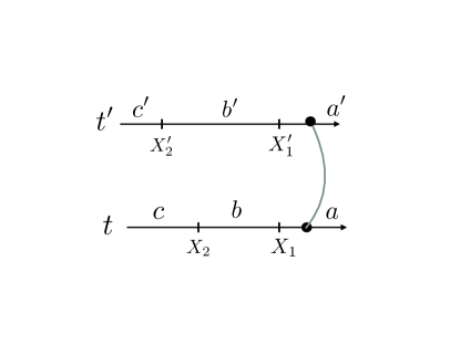
Note that the first term $\lambda_{aa}$ correspond to an event where the same particle is rightmost both at $t$ and $t^{\prime}$, while the second one $\lambda_{ac^{\prime}}\lambda_{ca^{\prime}}$ corresponds to an event where the righmost particle has changed, and in both cases the middle interval ($b$ and $b^{\prime}$) has remained empty. This is illustrated in Fig. 3.

Using the second relation in (112) the r.h.s of (120) can be rewritten as

$$\left(e^{-z_{1}}+e^{-z^{\prime}_{1}}-\Phi(z_{1},z^{\prime}_{1};\tau)+(\Phi(z_{1},z^{\prime}_{2};\tau)-e^{-z^{\prime}_{2}})(\Phi(z_{2},z^{\prime}_{1};\tau)-e^{-z_{2}}))\right)e^{-\Phi(z_{2},z^{\prime}_{2};\tau)}$$ (121)

Now taking four derivatives we obtain the joint PDF of the max and second max at two times, $q(z_{1},z_{2},z^{\prime}_{1},z^{\prime}_{2})$ in the variables $z_{i},z^{\prime}_{i}$,

$$q(z_{1},z_{2},z^{\prime}_{1},z^{\prime}_{2};\tau)=\partial_{z_{1}}\partial_{z^{\prime}_{1}}\partial_{z_{2}}\partial_{z^{\prime}_{2}}\text{Eq. \eqref{equiv12}}=\partial_{z_{1}}\partial_{z^{\prime}_{1}}\partial_{z_{2}}\partial_{z^{\prime}_{2}}\bigg{(}(\Phi(z_{1},z^{\prime}_{2};\tau)\Phi(z_{2},z^{\prime}_{1};\tau)-\Phi(z_{1},z^{\prime}_{1};\tau))e^{-\Phi(z_{2},z^{\prime}_{2};\tau)}\bigg{)}$$ (122)

as we see that the contributions of the additional exponentials vanish. This is the result (106) announced above. This derivation is different, but equivalent to the one given in the Appendix D.

Figure 3: Illustration of the two cases in (119) which occur in the calculation of the two time maximum and second maximum CDF in (120). Top: first case. Left: the rightmost particle at $t$ remains so at $t^{\prime}$. Right: the values of the occupation numbers defined in the text, corresponding to this event. Since they are independent Poisson distributed, see Eq. (114), this case leads to the term $\lambda_{aa^{\prime}}$ in (120). Bottom: second case. Left: the rightmost particle at $t$ is different from the rightmost at $t^{\prime}$. Since by definition of the CDF in (120) the middle interval is always empty (in both cases), these particles come from $c,c^{\prime}$ as illustrated. Right: the values of the occupation numbers corresponding to this event. This case leads to the term $\lambda_{ac^{\prime}}\lambda_{ca^{\prime}}$ in (120).

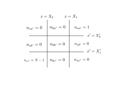
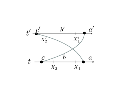
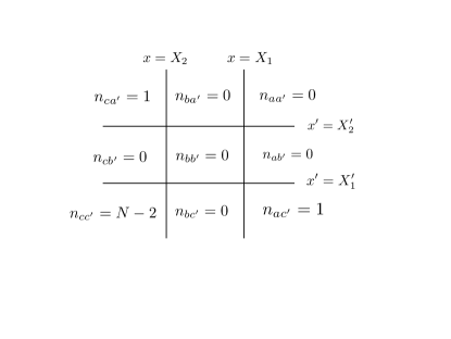
Another observable of interest, related to the two-time maximum, is the joint PDF of $n_{X_{1}}$ and $n^{\prime}_{X^{\prime}_{1}}$, where $n_{X}$ is the number of particules with $x_{i}(t)>X$ and $n^{\prime}_{X^{\prime}}$ is the number of particules with $x^{\prime}_{i}(t)>X^{\prime}$. One has

$$n_{X_{1}}=n_{aa^{\prime}}+n_{ab^{\prime}}+n_{ac^{\prime}}=n_{aa^{\prime}}+m$$ (123)

$$n^{\prime}_{X_{1}}=n_{aa^{\prime}}+n_{ba^{\prime}}+n_{ca^{\prime}}=n_{aa^{\prime}}+m^{\prime}$$ (124)

where $m$, $m^{\prime}$ are two independent Poisson variables, independent of $n_{aa^{\prime}}$, and of mean $\lambda=\lambda_{ab^{\prime}}+\lambda_{ac^{\prime}}$ and $\lambda^{\prime}=\lambda_{ba^{\prime}}+\lambda_{ca^{\prime}}$, respectively. The couple $n_{X_{1}},n^{\prime}_{X^{\prime}_{1}}$ thus obeys a bivariate Poisson distribution. Note that bivariate Poisson distributions also appear in the two-time counting statistics in the bulk, as discussed in [28]. Its distribution is

$${\rm Prob}(n_{X_{1}}=n_{1},n^{\prime}_{X^{\prime}_{1}}=n^{\prime}_{1}) = \sum_{n_{aa}=0}^{\min(n_{1},n^{\prime}_{1})}\frac{\lambda^{n_{1}-n_{aa}}}{(n_{1}-n_{aa})!}\frac{(\lambda^{\prime})^{n^{\prime}_{1}-n_{aa}}}{(n^{\prime}_{1}-n_{aa})!}\frac{\lambda_{aa}^{n_{aa}}}{n_{aa}!}e^{-\lambda-\lambda^{\prime}-\lambda_{aa}}$$ (125)

$$= \frac{(-1)^{n_{1}}}{n_{1}!}\frac{1}{n^{\prime}_{1}!}\lambda_{aa}^{n_{1}}(\lambda^{\prime})^{n_{1}^{\prime}-n_{1}}U(-n_{1},1-n_{1}+n^{\prime}_{1},-\frac{\lambda\lambda^{\prime}}{\lambda_{aa}})e^{-\lambda-\lambda^{\prime}-\lambda_{aa}}$$ (126)

where $U$ is the confluent hypergeometric function and

$$\lambda=e^{-z_{1}}-g(z_{1},z^{\prime}_{1};\tau)\quad,\quad\lambda^{\prime}=e^{-z^{\prime}_{1}}-g(z_{1},z^{\prime}_{1};\tau)\quad,\quad\lambda_{aa}=g(z_{1},z^{\prime}_{1};\tau)$$ (127)

with $\lambda+\lambda^{\prime}+\lambda_{aa}=\Phi(z_{1},z^{\prime}_{1};\tau)=e^{-z_{1}}\phi_{\tau}(z_{1}^{\prime}-z_{1})$. The characteristic function is

$$\langle e^{u_{1}n_{X_{1}}+u^{\prime}_{1}n_{X^{\prime}_{1}}}\rangle=e^{\lambda_{aa}(e^{u_{1}+u^{\prime}_{1}}-1)+\lambda(e^{u_{1}}-1)+\lambda^{\prime}(e^{u^{\prime}_{1}}-1)}$$ (128)

One obtains in particular the two time covariance of the number of particles

$${\rm Cov}(n_{X_{1}},n^{\prime}_{X^{\prime}_{1}})=\lambda_{aa}=g(z_{1},z^{\prime}_{1};\tau)=e^{-z_{1}}+e^{-z^{\prime}_{1}}-\Phi(z_{1},z^{\prime}_{1};\tau)$$ (129)

where we recall the asymptotics of the function $g$ (see Appendix B)

$$g(z_{1},z^{\prime}_{1};\tau)\simeq e^{-\max(z_{1},z^{\prime}_{1})}\quad,\quad\tau\to 0$$ (130)

$$g(z_{1},z^{\prime}_{1};\tau)=e^{-z_{1}}e^{-(z^{\prime}_{1}-z_{1}+\tau)^{2}/(4\tau)}\chi_{\tau}(z^{\prime}_{1}-z_{1})\quad,\quad\tau\to+\infty$$ (131)

where the large $\tau$ behavior of $\chi_{\tau}(z)$ is given in (57).

One can further study the joint PDF of $n_{X_{1}},n_{X_{2}},n^{\prime}_{X^{\prime}_{1}},n^{\prime}_{X^{\prime}_{2}}$. It is a multivariate Poisson distribution, which can be obtained from (114), with in addition to (123)

$$n_{X_{2}}=n_{X_{1}}+n_{ba^{\prime}}+n_{bb^{\prime}}+n_{bc^{\prime}}$$ (132)

$$n^{\prime}_{X_{2}}=n^{\prime}_{X^{\prime}_{1}}+n_{ab^{\prime}}+n_{bb^{\prime}}+n_{cb^{\prime}}$$ (133)

Its characteristic function can be easily written as above, but we will not pursue this here. One can simply give the two-time covariance of the number of particles in $[X_{2},X_{1}]$ at $t$ and in $[X^{\prime}_{2},X^{\prime}_{1}]$ at $t^{\prime}$, obtained as

$${\rm Cov}\left((n_{X_{2}}-n_{X_{1}})(n^{\prime}_{X^{\prime}_{2}}-n^{\prime}_{X^{\prime}_{1}})\right) \simeq {\rm Var}\left(n_{bb^{\prime}}\right)=\lambda_{bb^{\prime}}$$ (134)

$$= g(z_{2},z^{\prime}_{2};\tau)-g(z_{1},z^{\prime}_{2};\tau)-g(z_{2},z^{\prime}_{1};\tau)+g(z_{1},z^{\prime}_{1};\tau)$$ (135)

using (115).

Subcase with only two disjoint intervals, and two-time joint CDF of the second maximum. A subcase of the above result (114) is obtained by taking $X_{1},X^{\prime}_{1}\to+\infty$. One can then denote $X_{2}=X$ and $X^{\prime}_{2}=X^{\prime}$. This amounts to divide the line into two disjoint intervals (b) $x>X$, (c) $x<X$ at time $t$, and into two disjoint intervals (b) $x>X$, (c) $x<X$ at time $t^{\prime}$. In the large $N$ limit, denoting $z,z^{\prime}$ the rescaled coordinates, one obtains the PDF

$${\rm Prob}(n_{bb^{\prime}},n_{bc^{\prime}},n_{cb^{\prime}})=\frac{\lambda_{bb^{\prime}}^{n_{bb^{\prime}}}\,\lambda_{bc^{\prime}}^{n_{bc^{\prime}}}\lambda_{cb^{\prime}}^{n_{cb^{\prime}}}}{n_{bb^{\prime}}!n_{bc^{\prime}}!n_{cb^{\prime}}!}e^{-\Phi(z,z^{\prime},\tau)}$$ (136)

with

$$\lambda_{bb^{\prime}}=g(z,z^{\prime};\tau)\quad,\quad\lambda_{bc^{\prime}}=e^{-z}-g(z,z^{\prime};\tau)\quad,\quad\lambda_{cb^{\prime}}=e^{-z^{\prime}}-g(z,z^{\prime};\tau)$$ (137)

e.g. from (115) taking $z_{1},z^{\prime}_{1}\to+\infty$, since the $g$ function vanishes for any positive infinite argument (the other $\lambda_{ii^{\prime}}$ vanish and the corresponding $n_{ii^{\prime}}$ are frozen to $0$). Note that the counting statistics discussed above for $n_{aa}$, $m$ and $m^{\prime}$ in (123) is also recovered setting $(z,z^{\prime})=(z_{1},z^{\prime}_{1})$, $bb^{\prime}=aa^{\prime}$, $\lambda_{bc^{\prime}}=\lambda$ and $\lambda_{cb^{\prime}}=\lambda^{\prime}$.

The two-interval counting statistics (136), (137) allows to obtain some two-time distributions. First, of course, the two time joint CDF of the maximum is recovered as ${\rm Prob}(n_{bb^{\prime}}=0,n_{bc^{\prime}}=0,n_{cb^{\prime}}=0)$, setting $(z,z^{\prime})=(z_{1},z^{\prime}_{1})$. The two time joint CDF of the second maximum can also be obtained. Recall that in Section (2.3) we noted that for a single time the event $X^{(2)}(t)<X$ is equivalent to $n_{X}=0,1$. Here one has $n_{X}=n_{bb^{\prime}}+n_{bc^{\prime}}$ and $n^{\prime}_{X^{\prime}}=n_{bb^{\prime}}+n_{cb^{\prime}}$. Hence the event $X^{(2)}(t)<X$ and $X^{(2)}(t^{\prime})<X^{\prime}$ corresponds to $n_{X}=0,1$ and $n^{\prime}_{X^{\prime}}=0,1$, which corresponds to the union of events $(n_{bb^{\prime}},n_{bc^{\prime}},n_{cb^{\prime}})\in\{(0,0,0),(1,0,0),(0,1,0),(0,0,1),(0,1,1)\}$. This leads to the two time joint CDF of the second maximum

$${\rm Prob}(X^{(2)}(t)<X,X^{(2)}(t^{\prime})<X^{\prime})=1+\lambda_{bb^{\prime}}+\lambda_{bc^{\prime}}+\lambda_{cb^{\prime}}+\lambda_{bc^{\prime}}\lambda_{cb^{\prime}}$$ (138)

$$=\left(1+e^{-z}+e^{-z^{\prime}}-g(z,z^{\prime};\tau)+(e^{-z}-g(z,z^{\prime};\tau))(e^{-z^{\prime}}-g(z,z^{\prime};\tau))\right)e^{-\Phi(z,z^{\prime};\tau)}$$

$$=\left(1+\Phi(z,z^{\prime};\tau)+(\Phi(z,z^{\prime};\tau)-e^{-z^{\prime}})(\Phi(z,z^{\prime};\tau)-e^{-z})\right)e^{-\Phi(z,z^{\prime};\tau)}$$

Note that one can also find the two-time joint PDF of the second maximum from (120), as

$$q(z_{2},z^{\prime}_{2};\tau)=\int_{z_{2}}^{+\infty}dz_{1}\int_{z^{\prime}_{2}}^{+\infty}dz^{\prime}_{1}\partial_{z_{1}}\partial_{z^{\prime}_{1}}{\cal Q}(z_{1},z_{2},z^{\prime}_{1},z^{\prime}_{2})={\cal Q}(z_{2},z_{2},z^{\prime}_{2},z^{\prime}_{2})$$ (139)

$${\cal Q}(z_{1},z_{2},z^{\prime}_{1},z^{\prime}_{2})=\partial_{z_{2}}\partial_{z^{\prime}_{2}}\text{Eq. \eqref{equiv12}}$$ (140)

since the boundary terms at infinity do not contribute as the function $g$ vanish when any $z$ argument goes to $+\infty$. (beware that $z_{1}=z_{2}$ and $z^{\prime}_{1}=z^{\prime}_{2}$ should be taken only after taking the two derivatives $\partial_{z_{2}}\partial_{z^{\prime}_{2}}$). We have checked that this calculation gives the same result as taking $\partial_{z_{2}}\partial_{z^{\prime}_{2}}$ on the CDF (138).

The above calculation can be extended to obtain the two time joint CDF of the $k$-th maximum for any $k$. One must simply enumerate all the values of the triplet $(n_{bb^{\prime}},n_{bc^{\prime}},n_{cb^{\prime}})$ such that $n_{X}\in\{0,1,\dots,k-1\}$ and $n^{\prime}_{X^{\prime}}\in\{0,1,\dots,k-1\}$. A similar method yields the joint PDF of second maximum at $t$ and main maximum at $t^{\prime}$, or any other combination.

Finally, all the calculations in this Section can be extended to any number of times, any rank order and any number of intervals, although it quickly becomes tedious. This is sketched in Appendix E where we give explicit formula e.g. for the joint PDF of the two-time three first maxima, and the three time first two maxima.

7   Continuous time observables and rescaled process

7.1   Probability that the maximum remains below some curve for $t\in[t_{1},t_{2}]$

The multi-time joint PDF formula (23) is asking for a ”path integral” generalization. Given again the maximum process $X(t)=X_{N}(t)=\max_{i=1,\dots,N}x_{i}(t)$, an interesting observable in that respect, which we study in this subsection, is

$${\rm Prob}(X(t)<M(t)~{},~{}\forall t\in[t_{1},t_{2}])$$ (141)

upon proper rescaling of $X,M$ and $t_{2}-t_{1}$.

Let us make the following preliminary observations. Consider $n=2$ and the factorized form (39). Considering $z_{1}$ and $z_{2}$ as random variables whose CDF is $Q_{<<}$ in (42), the factorization implies that for any real $a,z$

$${\rm Prob}(\max(z_{1},z_{2}-a)<z)=e^{-e^{-z}\phi_{\tau}(a)}$$ (142)

Hence the random variable $\max(z_{1},z_{2}-a)$ for fixed $a$ is itself a Gumbel random variable, but shifted by $\log\phi_{\tau}(a)$ (a deterministic quantity). The equation (142) gives another nice interpretation to the function $\phi_{\tau}(a)$. Recall from Section 4.1.7 that the factorized form (39) does not imply that the PDF of $z_{1}$ conditioned to a given value of $z_{2,1}$ is Gumbel (its precise form is a bit different, see (76)).

For the original maximum process, the property (142) implies that the random variable $\max(X(t_{1}),X(t_{2})-M)$, when properly scaled (and where $M$ and $t_{2}-t_{1}$ are properly scaled) is also a shifted Gumbel random variable.

Clearly the property (142) extends to any number of times and for any $n\geq 2$

$$\max(z_{1},z_{2}-a_{2},\dots,z_{n}-a_{n})\quad\text{equal in law to}\quad G+\log\phi_{\tau_{2,1},\dots,\tau_{n,n-1}}(a_{2},a_{3,2},\dots,a_{n,n-1})$$ (143)

where $G$ is a Gumbel random variable.

To take the continuum limit one must consider the rescaled process. For this one must fix one time $t_{1}$, and defines the rescaled maximum process (or extremal process) $z(\tau)$ (a function of the rescaled time $\tau$, which lives in the vicinity of time $t_{1}$) by the equivalence at large $N$

$$X(t)\simeq\sqrt{2t\log N}(1+\frac{z(\tau)+c_{N}}{2\log N})\quad,\quad t-t_{1}=t_{1}\frac{\tau}{\log N}$$ (144)

or, more properly as the process

$$z(\tau)=\lim_{N\to+\infty}\left((2\log N)\left(\frac{X(t)}{\sqrt{2t\log N}}|_{t=t_{1}(1+\frac{\tau}{\log N})}-1\right)-c_{N}\right)$$ (145)

Such limits (and more general max stable processes) were considered rigorously in the statistics and probability literature, starting with the seminal work [15]. The one-time distribution of the process $z(\tau)$ is the Gumbel distribution. In the previous part of the paper we have studied the $n$ time CDF’s, $e^{-\Phi}$, of the process $z(\tau)$.

Let us return to the observable (141) and choose to scale

$$M(t)=X_{1}+\sqrt{\frac{t_{1}}{2\log N}}(m(\tau)+\tau)\quad,\quad X_{1}=\sqrt{2t_{1}\log N}(1+\frac{z_{1}+c_{N}}{2\log N})\quad,\quad\tau=\frac{t-t_{1}}{t_{1}}\log N$$ (146)

where $m(\tau)$ is any function with $m(0)=0$. Then one has at large $N$

$${\rm Prob}(X(t)<M(t)~{},~{}\forall t\in[t_{1},t_{2}])\simeq{\rm Prob}(z(\tau)<z_{1}+m(\tau)~{},~{}\forall\tau\in[0,\tau_{2,1}])$$ (147)

Now we can guess the continuum limit from Eq. (24). Indeed $\Phi$ is the expectation of $(1-\prod_{i=1}^{n}\theta_{y_{i}<z_{i}})$ over a Brownian with diffusion coefficient $D=2$ and drift $-1$, started at $y_{1}$ which is distributed with $e^{-y_{1}}$. The conjecture is thus

$${\rm Prob}(z(\tau)<z_{1}+m(\tau)~{},~{}\forall\tau\in[0,\tau_{2,1}])=e^{-\Psi(z_{1};\tau_{2,1};m(\tau))}$$ (148)

with

$$\Psi(z_{1};\tau_{2,1};m(\tau))=\int dye^{-y_{1}}\left(1-\theta(z_{1}-y_{1}){\rm Prob}(y_{1}+\sqrt{2}B(\tau)-\tau<z_{1}+m(\tau)~{},~{}\forall\tau\in[0,\tau_{2,1}])\right)$$ (149)

where $B(\tau)$ is a standard Brownian. So it is expressed in terms of the probability that the above mentioned Brownian does not hit the moving point $z_{1}+m(\tau)$. One sees that, shifting $y_{1}\to y_{1}+z_{1}$, one has

$$\Psi(z_{1},\tau_{2,1};m(\tau))=e^{-z_{1}}\Psi(\tau_{2,1};m(\tau))$$ (150)

$$\Psi(\tau_{2,1};m(\tau))=\int dye^{-y_{1}}\left(1-\theta(-y_{1}){\rm Prob}(y_{1}+\sqrt{2}B(\tau)-\tau<m(\tau)~{},~{}\forall\tau\in[0,\tau_{2,1}])\right)$$ (151)

Hence we can rewrite (148) as

$${\rm Prob}(z(\tau)-m(\tau)<z_{1}~{},~{}\forall\tau\in[0,\tau_{2,1}])=e^{-e^{-z_{1}}\Psi(\tau_{2,1};m(\tau))}$$ (152)

which implies that the random variable

$$\max_{\tau\in[0,\tau_{2,1}]}(z(\tau)-m(\tau))\quad\text{equal in law to}\quad G+\log\Psi(\tau_{2,1};m(\tau))$$ (153)

where $G$ is a Gumbel random variable. This is the continuum limit of (143). A scaled version can then be deduced for $X(t)-M(t)$.

One can derive this formula in the case where $m(\tau)=(w-1)\tau$ is a linear function of $\tau$. This is done in Appendix (F.2). In that case we have, with $y_{1}<0$

$${\rm Prob}(y_{1}+\sqrt{2}B(\tau)-\tau<(w-1)\tau~{},~{}\forall\tau\in[0,\tau_{2,1}])={\rm Prob}({\sf T}^{-w}_{-y_{1}}>\tau_{2,1})$$ (154)

where ${\sf T}^{-w}_{z}$ is the first passage time at level $z>0$ for a Brownian starting at the origin with drift $-w$ and diffusion coefficient $D=2$ (see Appendix F.1). This leads to

$${\rm Prob}(z(\tau)-(w-1)\tau<z_{1}~{},~{}\forall\tau\in[0,\tau_{2,1}])=e^{-e^{-z_{1}}\Psi_{w}(\tau_{2,1})}$$ (155)

with (changing variable to $y=-y_{1}$)

$$\Psi_{w}(\tau)=\int dye^{y}(1-\theta(y){\rm Prob}({\sf T}^{-w}_{y}>\tau))$$ (156)

This function can be computed explicitly for any $w$, the result is given in (309) in Appendix (F.2). Here we only display the result for $w=1$, i.e. for $m(\tau)=0$, which reads

$$\Psi_{1}(\tau)=\frac{1}{2}(\tau+2)\text{erfc}\left(\frac{\sqrt{\tau}}{2}\right)-\tau-\frac{e^{-\tau/4}\sqrt{\tau}}{\sqrt{\pi}}$$ (157)

which implies that $\max_{\tau\in[0,\tau_{2,1}]}z(\tau)$ is a Gumbel variable shifted by $\log\Psi_{1}(\tau_{2,1})$.

7.2   Running maximum and arrival time of first particle: one-time distributions

Let us first consider a single standard Brownian $x(t)$, with $r(t)=\max_{0\leq t^{\prime}\leq t}x(t^{\prime})$ its running maximum, and the CDF for $R_{1}>0$

$${\rm Prob}(r(t_{1})<R_{1})={\rm Prob}(T_{R_{1}}>t_{1})={\cal P}_{1}$$ (158)

where $T_{R}$ is the first passage time of the standard Brownian at level $R\geq 0$. It is given by (see Appendix F.1)

$${\cal P}_{1}={\rm Prob}(T_{R_{1}}>t_{1})=\int_{-\infty}^{R_{1}}dx_{1}(\frac{e^{-\frac{x_{1}^{2}}{2t_{1}}}}{\sqrt{2\pi t_{1}}}-\frac{e^{-\frac{(x_{1}-2R_{1})^{2}}{2t_{1}}}}{\sqrt{2\pi t_{1}}})$$ (159)

which is the probability that the Brownian with an absorbing wall at $R_{1}$ has survived up to $t_{1}$.

Let us now consider the running maximum $R(t)$ for $N$ identical standard Brownian motions starting from the origin

$$R(t)=\max_{0\leq t^{\prime}\leq t}X(t)=\max_{i}r_{i}(t)\quad,\quad r_{i}(t)=\max_{0\leq t^{\prime}\leq t}x_{i}(t^{\prime})$$ (160)

Let us first study the one-time CDF of the running maximum (which is a standard calculation but which sets the stage for the multi-time generalization given below). It is given by

$${\rm Prob}(R(t_{1})<R_{1})={\rm Prob}(r(t_{1})<R_{1})^{N}={\rm Prob}(T_{R_{1}}>t_{1})^{N}={\rm Prob}(T^{\rm min}_{R_{1}}>t_{1})$$ (161)

where the last term is equal to the probability that the minimum of the first passage times $T^{\rm min}_{R_{1}}=\min_{i}T^{i}_{R_{1}}$ at $R_{1}$ of $N$ identical copies is larger than $t_{1}$. This is also the arrival time at $R_{1}$ of the first particle, an important quantity.

At large $N$, we will scale $R_{1}$ as usual as $R_{1}=\sqrt{2t_{1}\log N}(1+\frac{z_{1}+c_{N}}{2\log N})$ so that $1-{\cal P}_{1}=O(1/N)$ and

$${\rm Prob}(R(t_{1})<R_{1})={\rm Prob}(T_{R_{1}}>t_{1})^{N}\simeq e^{-N(1-{\cal P}_{1})}$$ (162)

Let us now estimate, from (159), using similar manipulations as in Appendix A

$$N(1-{\cal P}_{1})=N\int dx_{1}\frac{e^{-\frac{x_{1}^{2}}{2t_{1}}}}{\sqrt{2\pi t_{1}}}\left(1-\theta(R_{1}-x_{1})\left(1-e^{-\frac{2R_{1}(R_{1}-x_{1})}{t_{1}}}\right)\right)$$ (163)

$$\simeq\int dy_{1}e^{-y_{1}}(1-\theta(z_{1}-y_{1})(1-e^{-2(z_{1}-y_{1})}))$$

$$=e^{-z_{1}}\int dye^{y}(1-\theta(y)(1-e^{-2y}))=e^{-z_{1}}(\int_{y>0}e^{y}+\int_{y<0}e^{-y})=2e^{-z_{1}}$$ (164)

where we have changed variables denoting $x_{1}=\sqrt{2t_{1}\log N}(1+\frac{y_{1}+c_{N}}{2\log N})$, followed by $y_{1}=z_{1}-y$. Note that the term $e^{-y_{1}}-e^{2z_{1}-y_{1}}$ upon expanding the middle line can be interpreted as the stationary measure of the diffusion with negative drift in presence of a hard wall at $z_{1}$. At the end, not surprisingly, at large $N$ the running maximum has a Gumbel distribution

$${\rm Prob}(R(t_{1})<R_{1})\simeq e^{-2e^{-z_{1}}}\simeq{\rm Prob}(X(t_{1})<R_{1})^{2}$$ (165)

with, however, a shift as compared to the instantaneous maximum, i.e. $z_{1}=G+\log 2$.

Since one can read (161) both ways (i.e. for the running maximum or for the arrival time of the first particle), the above result also implies that

$${\rm Prob}(T^{\rm min}_{R_{1}}>t_{1})\simeq e^{-2e^{-z_{1}}}$$ (166)

where the arrival time of the first particle (see Appendix (F.3) for details)

$$T^{\rm\min}_{R_{1}}=t_{1}=\frac{R_{1}^{2}}{2\log N}(1-\frac{z_{1}+c_{N}}{\log N}))$$ (167)

where from (166) $z_{1}=G+\log 2$ and $G$ is Gumbel distributed.

7.3   Running maximum: two-time distribution

.

We can now ask about the two-time joint CDF of the running maximum, at two given times, $t_{2}>t_{1}$

$${\rm Prob}(R(t_{1})<R_{1},R(t_{2})<R_{2})={\rm Prob}(r(t_{1})<R_{1},r(t_{2})<R_{2})^{N}={\rm Prob}(T_{R_{1}}>t_{1},T_{R_{2}}>t_{2})^{N}$$ (168)

with $R_{2}>R_{1}$, which now involves the two-time joint ”CDF” of the first passage times of a single Brownian at $R_{1}$ and $R_{2}$. The latter is given by

$${\cal P}={\rm Prob}(T_{R_{1}}>t_{1},T_{R_{2}}>t_{2})=\int_{-\infty}^{R_{1}}dx_{1}\int_{-\infty}^{R_{2}}dx_{2}(\frac{e^{-\frac{x_{1}^{2}}{2t_{1}}}}{\sqrt{2\pi t_{1}}}-\frac{e^{-\frac{(x_{1}-2R_{1})^{2}}{2t_{1}}}}{\sqrt{2\pi t_{1}}})(\frac{e^{-\frac{(x_{2}-x_{1})^{2}}{2(t_{2}-t_{1})}}}{\sqrt{2\pi(t_{2}-t_{1})}}-\frac{e^{-\frac{(x_{2}+x_{1}-2R_{2})^{2}}{2(t_{2}-t_{1})}}}{\sqrt{2\pi(t_{2}-t_{1})}})$$ (169)

which is the probability that the Brownian with an absorbing wall at $R_{1}$ for $t\in[0,t_{1}]$ and an absorbing wall at $R_{2}$ for $t\in[t_{1},t_{2}]$ has survived up to $t_{2}$.

Note that for $N=1$, i.e. for a single Brownian $x(t)$, the two time PDF of $R(t_{1})=R_{1}$ and $R(t_{2})=R_{2}$ was obtained in [29] (their Eq. (6)). This PDF vanishes for $R_{2}<R_{1}$ since the running maximum can only increase with time, but there is however a $\delta(R_{2}-R_{1})$ component in the PDF. Its weight corresponds to the probability that $x(t)$ reaches $R(t_{1})$ at some time before $t_{1}$, but never crosses again the level $R(t_{1})$ for $t\in]t_{1},t_{2}]$, so that $R(t_{2})=R(t_{1})$. As we will see below there is a similar feature for $N>1$.

In the large $N$ limit we will scale as usual

$$R_{i}=\sqrt{2t_{i}\log N}(1+\frac{z_{i}+c_{N}}{2\log N})\quad,\quad t_{2}-t_{1}=t_{1}\frac{\tau}{\log N}$$ (170)

and insert in (169). The calculation is sketched in the Appendix F.4. One finds that at large $N$ the two time CDF of the running maximum takes the form, for $R_{1}\leq R_{2}$, which corresponds to $z_{2,1}=z_{2}-z_{1}\geq-\tau$,

$${\rm Prob}(R(t_{1})<R_{1},R(t_{2})<R_{2})\simeq e^{-\Gamma(z_{1},z_{2};\tau)}=e^{-e^{-z_{1}}\gamma_{\tau}(z_{21})}$$ (171)

where for $z\geq-\tau$

$$\gamma_{\tau}(z)=\int dy_{1}\int dy_{2}\,e^{y_{1}}\frac{e^{-\frac{(z-y_{2,1}+\tau)^{2}}{4\tau}}}{\sqrt{4\pi\tau}}(1-\theta(y_{1})\theta(y_{2})(1-e^{-2y_{1}})(1-e^{-\frac{(z+\tau+y_{1})y_{2}}{\tau}}))$$ (172)

a generalization of (164). It turns out that this integral can be computed explicitly (see Appendix F.4) and one finds

$$\gamma_{\tau}(z)=2\text{erf}\left(\frac{\tau+z}{2\sqrt{\tau}}\right)+e^{-z}\text{erfc}\left(\frac{z-\tau}{2\sqrt{\tau}}\right)+e^{2\tau+z}\text{erfc}\left(\frac{3\tau+z}{2\sqrt{\tau}}\right)\quad,\quad z\geq-\tau$$ (173)

Since the running maximum always increases, for $R_{2}\leq R_{1}$ one has

$${\rm Prob}(R(t_{1})<R_{1},R(t_{2})<R_{2})={\rm Prob}(R(t_{2})<R_{2})\simeq e^{-2e^{-z_{2}}}$$ (174)

The boundary case $R_{2}=R_{1}$ corresponds to $z_{1}=z_{2}+\tau$, i.e. $z_{2,1}=-\tau$. Then we see that (174) is consistent with the boundary value $\gamma_{\tau}(z=-\tau)=2e^{\tau}$ which one obtains from (173). Thus one can extend (171) to any $z_{2,1}$ if one defines

$$\gamma_{\tau}(z)=2e^{-z}\quad\text{for}\quad z\leq-\tau$$ (175)

One can check that that $\gamma_{\tau}(z)$ is a decreasing function of $z$, with $\gamma_{\tau}(z)>\phi_{\tau}(z)$, which is consistent with the fact that the running maximum is always larger than the instantaneous maximum.

Let us study the asymptotic behaviors of $\gamma_{\tau}(z)$. The large $z$ behavior is

$$\gamma_{\tau}(z)=2+e^{-\frac{(z+\tau)^{2}}{4\tau}}\frac{16\tau^{5/2}}{\sqrt{\pi}z^{3}}(1-\frac{3\tau}{z}+\frac{2\tau(5\tau-6)}{z^{2}}+O(z^{-3}))\quad,\quad z\to+\infty$$ (176)

The limit $\gamma_{\tau}(+\infty)=2$ is consistent with the one time result (165). The large $\tau$ limit is

$$\gamma_{\tau}(z)=2(1+e^{-z})-e^{-\frac{\tau}{4}-\frac{z}{2}}\frac{16}{3\sqrt{\pi\tau}}(1-\frac{80+3z(4+3z)}{36\tau}+O(\tau^{-2}))\quad,\quad\tau\to+\infty$$ (177)

The asymptotic value $2(1+e^{-z})$ yields $e^{-e^{-z_{1}}\gamma_{\tau}(z_{21})}\to e^{-2e^{-z_{1}}}e^{-2e^{-z_{2}}}$, i.e. $R(t_{1})$ and $R(t_{2})$ become statistically independent and one recovers the product of the one-time distributions.

Consider now $z_{1}$ and $z_{2,1}=z_{2}-z_{1}$, i.e the scaled positions of the running maximum from (170), as random variables. Their exponential moments can be computed as in (249), replacing $\phi_{\tau}(z)$ by $\gamma_{\tau}(z)$. Similarly on has $1/\gamma_{\tau}(z)^{a+b}\to 2^{-(a+b)}$ as as $z\to+\infty$. Hence (48), as well as (50), hold with the replacement $\phi_{\tau}(z)$ by $\gamma_{\tau}(z)$. One notes from (175) that the combination which appears in these formula

$$1+\frac{\gamma_{\tau}^{\prime}(z)}{\gamma_{\tau}(z)}=0\quad\text{for}\quad z<-\tau$$ (178)

vanishes for $z<-\tau$, and converges to $1$ exponentially fast as $z\to+\infty$. However this combination vanishes discontinuously at $z=-\tau$. Indeed one finds

$$1+\frac{\gamma_{\tau}^{\prime}(z)}{\gamma_{\tau}(z)}|_{z=-\tau^{+}}={\rm Erfc}(\sqrt{\tau})$$ (179)

Hence the marginal PDF of $z=z_{2,1}=z_{2}-z_{1}$, which we denote by $\tilde{P}^{(2,1)}_{\tau}(z)$, now acquires a delta function part and is given by, for $z\geq-\tau$

$$\tilde{P}^{(2,1)}_{\tau}(z)=q_{\tau}\delta(z+\tau)+\partial_{z}^{2}\log\gamma_{\tau}(z)\quad,\quad q_{\tau}={\rm Erfc}(\sqrt{\tau})\quad,\quad z\geq-\tau$$ (180)

and vanishes for $z<-\tau$. The second term is smooth: it has a finite value $1-{\rm Erfc}(\sqrt{\tau})^{2}$ at $z=-\tau$, with positive first derivative, so $\tilde{P}^{(2,1)}_{\tau}(z)$ has a maximum for some $\tau$-dependent value of $z$. As explained above for $N=1$, the weight of the delta part in in (180) corresponds to the probability $q_{\tau}$ that $R(t_{2})=R(t_{1})$. Specifically it corresponds to events such that the running maximum $R(t_{1})$ was achieved by one particle at some time before $t_{1}$ and that all particles have remained below that level for $t\in[t_{1},t_{2}]$. Note that when $\tau\to 0$ the delta part in (180) dominate the smooth part. Finally the CDF of $z_{2,1}$ is given by

$${\rm Prob}(z_{2,1}<z)=1+\partial_{z}\log\phi_{\tau}(z)$$ (181)

and exhibits a jump $q_{\tau}$ at $z=-\tau$.

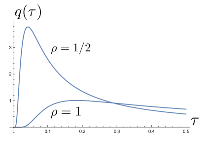
The PDF in (180) is plotted in Fig. 4 and has the following asymptotic behaviors. For fixed $\tau$ and $z\to+\infty$ it decays as

$$\tilde{P}^{(2,1)}_{\tau}(z)=e^{-\frac{(z+\tau)^{2}}{4\tau}}\frac{2\sqrt{\tau}}{z\sqrt{\pi}}\left(1-\frac{\tau}{z}+\frac{\tau(5\tau-2)}{z^{2}}+O(z^{-3})\right)\quad,\quad z\to+\infty$$ (182)

while for fixed $z$ and $\tau\to+\infty$ it behaves as

$$\tilde{P}^{2,1}_{\tau}(z)=\frac{1}{4\cosh^{2}(\frac{z}{2})}+\frac{e^{-\tau}}{\sqrt{\pi\tau}}\delta(z+\tau)+\frac{e^{-\frac{\tau}{4}}}{\sqrt{\pi\tau}}\left(\frac{3-\cosh(z)}{6\cosh^{3}(\frac{z}{2})}+O(\frac{1}{\tau})\right)\quad,\quad\tau\to+\infty$$ (183)

which should be compared with the result (58) for the instantaneous maximum. Hence at large $\tau$, $z_{2,1}$ is distributed again as the difference of two Gumbel random variables, the even moments have exactly the same limit as in (60), and the odd ones tend to zero.

Figure 4: Left: marginal PDF of $z=z_{2,1}=z_{2}-z_{1}$, the scaled distance traveled by the running maximum, with $R(t_{2})-R(t_{1})\simeq\sqrt{\frac{t_{1}}{2\log N}}(\tau+z)$. It is plotted for $\tau=1/2,1,2$ and vanishes discontinuously for $z<-\tau$. In addition there is a delta function at $z=-\tau$, not shown, of amplitude $q_{\tau}={\rm Erfc}(\sqrt{\tau})\approx 0.32,0.16,0.05$, corresponding to the event $R(t_{2})=R(t_{1})$, see (180). Right: its second moment $\langle z_{2,1}^{2}\rangle=D_{2}(\tau)$, plotted versus $\tau$. The first two terms in the small $\tau$ asymptotics (7.3), and the first three terms in the large $\tau$ asymptotics (186) are also plotted, together with the limiting value $\pi^{2}/3$. Convergence to the asymptotics is slower than for $A_{2}(\tau)$. Recall that $\pi^{2}/3-D_{2}(\tau)$, i.e. the curve reflected versus $\pi^{2}/3$ describes the two-time covariance of the running maximum, see Eq. (193).

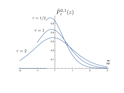
The integer moments of the random variable $z_{2,1}$ are obtained as, for $k\geq 1$

$$\langle z_{2,1}^{k}\rangle=D_{k}(\tau)=\int_{-\tau}^{+\infty}dzz^{k}P^{2,1}_{\tau}(z)=q_{\tau}(-\tau)^{k}+\int_{-\tau}^{+\infty}dzz^{k}\partial_{z}^{2}\log\gamma_{\tau}(z)$$ (184)

The function $D_{2}(\tau)$ is plotted in Fig. 4 using that formula. An alternative expression can be obtained upon integration by parts

$$\langle z_{2,1}^{k}\rangle=D_{k}(\tau)=(1-k)(-\tau)^{k}+k(k-1)\int_{-\tau}^{+\infty}dzz^{k-2}\log(\frac{\gamma_{\tau}(z)}{2})$$ (185)

where we have used (179) and $\gamma_{\tau}(-\tau)=2e^{\tau}$, $\gamma_{\tau}(+\infty)=2$ and that $\gamma^{\prime}_{\tau}(z)/\gamma_{\tau}(z)$ decays exponentially fast at $z\to+\infty$. For $k=1$ this implies that the first moment vanishes, $\langle z_{2,1}\rangle=0$, as it should since $\langle z_{1}\rangle=\langle z_{2}\rangle=\log 2+\gamma_{E}$ from the one-time result (165).

To obtain the large time asymptotics of the moments we use (183) (to a higher order, not shown). Inserting into (184) the last term of (183) leads to a convergent integral on $z\in]-\infty,+\infty[$. The term $q_{\tau}(-\tau)^{k}\simeq(-\tau)^{k}e^{-\tau}/\sqrt{\pi\tau}$ is subdominant as compared to the leading decay $\sim e^{-\tau/4}$. One finds $\langle z_{2,1}\rangle=D_{1}(\tau)=0$ and

$$\langle z_{2,1}^{2}\rangle=D_{2}(\tau)=\frac{\pi^{2}}{3}-\frac{16\sqrt{\pi}e^{-\tau/4}}{3\sqrt{\tau}}\left(1-\frac{\frac{20}{9}+\frac{\pi^{2}}{4}}{\tau}+\frac{\frac{364}{27}+\frac{5\pi^{2}}{3}+\frac{5\pi^{4}}{32}}{\tau^{2}}+O(\frac{1}{\tau^{3}})\right)$$ (186)

$$\langle z_{2,1}^{3}\rangle=D_{3}(\tau)=\frac{16\pi^{5/2}e^{-\tau/4}}{3\tau^{3/2}}(1-\frac{5}{12\tau}\left(16+3\pi^{2}\right)+\frac{\frac{1820}{27}+\frac{125\pi^{2}}{9}+\frac{61\pi^{4}}{32}}{\tau^{2}}+O(\frac{1}{\tau^{3}}))$$ (187)

$$\langle z_{2,1}^{4}\rangle=D_{4}(\tau)=\frac{7\pi^{4}}{15}-\frac{32\pi^{5/2}e^{-\tau/4}}{\sqrt{\tau}}\left(1-\frac{5}{36\tau}\left(16+9\pi^{2}\right)+\frac{\frac{364}{27}+\frac{25\pi^{2}}{3}+\frac{61\pi^{4}}{32}}{\tau^{2}}+O(\frac{1}{\tau^{3}})\right)$$ (188)

Note that the third moment of $z_{2}-z_{1}$, which is also the third cumulant vanishes at large $\tau$, as all the odd moments, and its leading order is one order lower than the corrections to the even moments.

Let us study now the close time asymptotics. At short time difference $\tau\ll 1$, we can scale

$$z_{2,1}=-\tau+w\sqrt{\tau}\quad,\quad w\geq 0$$ (189)

where $w$ is a $O(1)$ positive random variable. This is a bit different from the case of the instantaneous maximum. Upon this scaling we find that the PDF $p_{\tau}(w)$ of the random variable $w$ admits the following small $\tau$ expansion

$$p_{\tau}(w)=\left(1-\frac{2\sqrt{\tau}}{\sqrt{\pi}}(1-\frac{\tau}{3}+O(\tau^{2}))\right)\delta(w)+\sqrt{\tau}\,\text{erfc}\left(\frac{w}{2}\right)$$ (190)

$$+\tau^{3/2}\left(\frac{e^{-\frac{w^{2}}{4}}w\left(5\text{erfc}\left(\frac{w}{2}\right)-1\right)}{\sqrt{\pi}}+\frac{1}{2}\text{erfc}\left(\frac{w}{2}\right)\left(-\left(3w^{2}+2\right)\text{erfc}\left(\frac{w}{2}\right)+w^{2}+2\right)-\frac{4e^{-\frac{w^{2}}{2}}}{\pi}\right)+O(\tau^{5/2})$$

which is normalized to unity order by order in $\tau$. Since $\langle z_{2,1}\rangle=0$, one must have $\langle w\rangle=\int_{0}^{+\infty}dw\,w\,p_{\tau}(w)=\sqrt{\tau}$, which is indeed satisfied by (190) to the order displayed. Note that in the small $\tau$ limit $z_{2,1}$ has an intermittent behavior, it is equal to $-\tau$ with probability $1-O(\sqrt{\tau})$ (which corresponds to the event $R(t_{2})=R(t_{1})$) and is of order $O(\sqrt{\tau})$ with probability $O(\sqrt{\tau})$ (which corresponds to the event $R(t_{2})>R(t_{1})$).

From (190) one finds the small $\tau$ expansion of the moments of $z_{2,1}$ of lowest order, as well as the skewness $Sk$

$$\langle z_{2,1}^{2}\rangle=\langle z_{21}^{2}\rangle^{c}=D_{2}(\tau)=\tau\langle w^{2}\rangle-\tau^{2}=\tau\langle w^{2}\rangle^{c}=\frac{8}{3\sqrt{\pi}}\tau^{3/2}-\tau^{2}+\frac{8\left(4\sqrt{2}-5\right)}{15\sqrt{\pi}}\tau^{5/2}+O(\tau^{7/2})$$

$$\langle z_{2,1}^{3}\rangle=\langle z_{21}^{3}\rangle^{c}=D_{3}(\tau)=\tau^{3/2}\langle w^{3}\rangle-3\tau^{2}\langle w^{2}\rangle+2\tau^{3}=\tau^{3/2}\langle w^{3}\rangle^{c}$$ (191)

$$~{}~{}~{}~{}~{}~{}~{}~{}~{}~{}~{}~{}~{}~{}~{}~{}~{}~{}~{}~{}~{}~{}~{}~{}~{}~{}~{}~{}~{}~{}=3\tau^{2}-\frac{8\tau^{5/2}}{\sqrt{\pi}}+\frac{8\tau^{3}}{\pi}-\frac{8\left(4\sqrt{2}-5\right)\tau^{7/2}}{5\sqrt{\pi}}+O(\tau^{4})$$

$$Sk=\frac{D_{3}(\tau)}{D_{2}(\tau)^{3/2}}=\frac{9\sqrt{3}\pi^{3/4}}{16\sqrt{2}\tau^{1/4}}\bigg{(}1+\frac{(27\pi-64)\sqrt{\tau}}{24\sqrt{\pi}}+\left(-\frac{3}{2}-\frac{6\sqrt{2}}{5}+\frac{8}{3\pi}+\frac{135\pi}{128}\right)\tau+O(\tau^{3/2})\bigg{)}$$

The large and small $\tau$ asymptotics are shown in Fig. (4). As compared to $A_{2}(\tau)$, one needs larger values of $\tau$ (respectively smaller) to approximate the function by the first few terms of the series.

Finally, let us recall that in the original variables for the running maximum $R(t_{i})=R_{i}$, from (170) one has

$$R_{2}-R_{1}\simeq\sqrt{\frac{t_{1}}{2\log N}}(\tau+z_{2,1})\quad,\quad\tau=\frac{t_{2}-t_{1}}{t_{1}}\log N=O(1)$$ (192)

The one time distributions of $z_{1}$ and $z_{2}$ are shifted Gumbel, hence their variance are the same as for the instantaneous maximum, i.e. one has ${\rm Var}R_{1}={\rm Var}R_{2}\simeq\frac{t_{1}}{2\log N}\frac{\pi^{2}}{6}$. This leads to the two time covariance of the running maximum

$${\rm Cov}(R(t_{1}),R(t_{2}))\simeq\frac{t_{1}}{4\log N}(\frac{\pi^{2}}{3}-D_{2}(\tau))\simeq_{\tau\to+\infty}\frac{t_{1}}{4\log N}\frac{16\sqrt{\pi}e^{-\tau/4}}{3\sqrt{\tau}}$$ (193)

which can be compared to (72)

7.4   Arrival time of the first particle: two-time distribution

Consider now, for fixed $R_{2}>R_{1}$, the joint distribution of $T^{\rm min}_{R_{1}}$ and $T^{\rm min}_{R_{1}}$, the arrival times of the first particle respectively at $x=R_{1}$ et $x=R_{2}$. We can introduce again the rescaled variables $z_{1}$ and $z_{2}$ as

$$T^{\rm\min}_{R_{1}}=t_{1}=\frac{R_{1}^{2}}{2\log N}(1-\frac{z_{1}+c_{N}}{\log N}))$$ (194)

$$T^{\rm\min}_{R_{2}}=t_{2}=\frac{R_{2}^{2}}{2\log N}(1-\frac{z_{2}+c_{N}}{\log N}))$$ (195)

Clearly if $R_{2}$ and $R_{1}$ are sufficiently separated $z_{1}$ and $z_{2}$ (seen as random variables) will be two independent Gumbel variables, each with the one-time CDF (166). To see how close $R_{2}$ and $R_{1}$ must be so that non-trivial correlations exist we look at the ratio

$$\frac{t_{2}-t_{1}}{t_{1}}=\frac{R_{2}^{2}-R_{1}^{2}}{R_{1}^{2}}-\frac{z_{2}-z_{1}}{\log N}\frac{R_{2}^{2}}{R_{1}^{2}}+O(\frac{1}{(\log N)^{2}})$$ (196)

Since we want this ratio to be of order $1/\log N$ we need to choose

$$\frac{R_{2}-R_{1}}{R_{1}}=\frac{\rho}{2\log N}$$ (197)

where $\rho=O(1)$ is a fixed number. Hence we can approximate $\frac{R_{2}^{2}-R_{1}^{2}}{R_{1}^{2}}\simeq\frac{2(R_{2}-R_{1})}{R_{1}}$ in the first term in the r.h.s. of (196), and $R_{2}/R_{1}\simeq 1$ in the second term there, and our usual variable $\tau$ becomes

$$\tau=\frac{t_{2}-t_{1}}{t_{1}}\log N\simeq\rho-z_{2,1}$$ (198)

but we have to remember that $\tau$ it is now fluctuating. Hence the variable $\tau$ is related to the variable $z_{2,1}$ of the previous section. Note in particular that since $\tau>0$, one must have $z_{2,1}<\rho$.

We can now use the results of the previous section and obtain from (171), the joint ”CDF” of the first particules arrival times $T^{\rm min}_{R_{1}}$, $T^{\rm min}_{R_{2}}$, for fixed dimensionless distance $\rho>0$ defined in (197)

$${\rm Prob}(T^{\rm min}_{R_{1}}>t_{1},T^{\rm min}_{R_{2}}>t_{2}) = {\rm Prob}(R(t_{1})<R_{1},R(t_{2})<R_{2})$$ (199)

$$\simeq Q_{<<}(z_{1},z_{2})=e^{-e^{-z_{1}}\sigma_{\rho}(z_{2,1})}\quad,\quad\sigma_{\rho}(z)=\gamma_{\tau=\rho-z}(z)$$ (200)

where $Q_{<<}(z_{1},z_{2})$ is the CDF in the rescaled variables. For large $\rho$, using (177), one finds $Q_{<<}(z_{1},z_{2})\to e^{-2e^{-z_{1}}-2e^{-z_{2}}}$ which corresponds to two independent shifted Gumbel random variables, as expected.

In fact it is more convenient to eliminate $z_{2}$ and use $z_{1}$ and $\tau$ as the basic random variables. It means that we write

$$T^{\rm\min}_{R_{1}}=t_{1}=\frac{R_{1}^{2}}{2\log N}(1-\frac{z_{1}+c_{N}}{\log N})\quad,\quad\frac{T^{\rm\min}_{R_{2}}-T^{\rm\min}_{R_{1}}}{T^{\rm\min}_{R_{1}}}\simeq\frac{T^{\rm\min}_{R_{2}}-T^{\rm\min}_{R_{1}}}{(R_{1}^{2}/2\log N)}=\frac{\tau}{\log N}$$ (201)

hence $\tau$ has the interpretation of the (rescaled) delay time between detecting a first particle at $R_{1}$ and detecting a first particle at $R_{2}$ (which, of course, may not be the same particle). Note that in the second equation in (201), $T^{\rm\min}_{R_{1}}$ in the denominator can be approximated by its leading order value $R_{1}^{2}/2\log N$, to the same order at large $N$.

The random variables $z_{1}$ and $\tau>0$ defined in (201) are distributed with the joint PDF (using the change of variable (245) with $\partial_{z_{21}}=-\partial_{\tau}$)

$$q(z_{1},\tau)=-\partial_{\tau}(\partial_{z_{1}}+\partial_{\tau})e^{-e^{-z_{1}}\Sigma_{\rho}(\tau)}\quad,\quad\Sigma_{\rho}(\tau)=\gamma_{\tau}(\rho-\tau)\quad,\quad\rho>0\quad,\quad\tau>0$$ (202)

where the function $\Sigma_{\rho}(\tau)$ has the explicit form, from (173)

$$\Sigma_{\rho}(\tau)=2\text{erf}\left(\frac{\rho}{2\sqrt{\tau}}\right)+e^{\tau-\rho}\text{erfc}\left(\frac{\rho-2\tau}{2\sqrt{\tau}}\right)+e^{\rho+\tau}\text{erfc}\left(\frac{\rho+2\tau}{2\sqrt{\tau}}\right)$$ (203)

It obeys the identity $\Sigma_{\rho}(\tau)-\Sigma^{\prime}_{\rho}(\tau)=2\,\text{erf}\left(\frac{\rho}{2\sqrt{\tau}}\right)$. We recall that the parameter $\rho$ is defined in (197) and is proportional to the spatial separation of the two points $R_{1},R_{2}$ where the arrival times are measured.

Below we will need the small and large $\tau$ asymptotics of $\Sigma_{\rho}(\tau)$, which we now study. For $\tau\to 0$ at fixed $\rho$ one finds

$$\Sigma_{\rho}(\tau)=2+\frac{16\tau^{5/2}}{\sqrt{\pi}\rho^{3}}\left(1-\frac{12\tau}{\rho^{2}}+\frac{4\left(\rho^{2}+45\right)\tau^{2}}{\rho^{4}}+O\left(\tau^{3}\right)\right)\exp\left(-\frac{\rho^{2}}{4\tau}\right)$$ (204)

so that, for $\tau\to 0$ at fixed $\rho$ one has $\frac{\Sigma^{\prime}_{\rho}(\tau)}{\Sigma_{\rho}(\tau)}\to 0$ exponentially fast. To study large $\tau$ at fixed $\rho$ it is more convenient to write $\Sigma_{\rho}(\tau)$ in the equivalent form

$$\Sigma_{\rho}(\tau)=2e^{\tau-\rho}+2\text{erf}\left(\frac{\rho}{2\sqrt{\tau}}\right)+e^{\tau+\rho}\text{erfc}\left(\frac{2\tau+\rho}{2\sqrt{\tau}}\right)-e^{\tau-\rho}\text{erfc}\left(\frac{2\tau-\rho}{2\sqrt{\tau}}\right)$$ (205)

From it one obtains the large $\tau$ asymptotics

$$\Sigma_{\rho}(\tau)=2e^{\tau-\rho}+\frac{2\rho}{\sqrt{\pi\tau}}\left(1-\frac{\rho^{2}+6}{12\tau}+\frac{\rho^{4}+20\rho^{2}+120}{160\tau^{2}}+O(\tau^{-3})\right)$$ (206)

In that limit the following combination, useful below, vanishes as

$$1-\frac{\Sigma^{\prime}_{\rho}(\tau)}{\Sigma_{\rho}(\tau)}=e^{\rho-\tau}\,\text{erf}\left(\frac{\rho}{2\sqrt{\tau}}\right)+O(e^{-2\tau})=e^{\rho-\tau}\,\frac{\rho}{\sqrt{\pi\tau}}\left(1-\frac{\rho^{2}}{12\tau}+\frac{\rho^{4}}{160\tau^{2}}+O(\tau^{-3})\right)$$ (207)

Figure 5: Left: PDF $q(\tau)$ of the scaled time delay $\tau$ between the arrival of the first particles at $R_{1}$ and at $R_{2}$, with $\frac{T^{\rm\min}_{R_{2}}-T^{\rm\min}_{R_{1}}}{T^{\rm\min}_{R_{1}}}\simeq\frac{\tau}{\log N}$, for some values of the parameter $\rho$, with $\frac{R_{2}-R_{1}}{R_{1}}=\frac{\rho}{2\log N}$. Right: its second cumulant $\langle\tau^{2}\rangle_{c}=C_{2}(\rho)$, plotted versus $\rho$. The small $\rho$ asymptotics and the the limiting value $\pi^{2}/3$ at large $\rho$ are also shown.

Let us now turn to the exponential moments and to the marginal PDF of the delay time $\tau$. One finds, by a similar calculation as in (249),

$$\langle e^{-sz_{1}-b\tau}\rangle=-\Gamma(1+s)\int_{0}^{+\infty}d\tau e^{-b\tau}\partial_{\tau}\left((1-\frac{\Sigma^{\prime}_{\rho}(\tau)}{\Sigma_{\rho}(\tau)})\frac{1}{\Sigma_{\rho}(\tau)^{s}}\right)$$ (208)

For $b=0$, the integrand is a total derivative with boundary values $0$ at $\tau=+\infty$ and $2^{-s}$ at $\tau=0$ (from the above asymptotics), and one recovers the one time result, $\langle e^{-sz_{1}}\rangle=\Gamma(1+s)2^{-s}$. Inserting $s=0$ one finds the PDF $q(\tau)$ and the ”CDF” of the (scaled) delay time, i.e. the random variable $\tau$

$$q(\tau)=-\partial_{\tau}(1-\frac{\Sigma^{\prime}_{\rho}(\tau)}{\Sigma_{\rho}(\tau)})=\partial_{\tau}^{2}\log\Sigma_{\rho}(\tau)\quad,\quad{\rm Prob}(\tau>t)=1-\partial_{\tau}\log\Sigma_{\rho}(\tau)$$ (209)

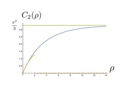
This PDF is plotted in Fig. 5. The PDF $q(\tau)$ vanishes exponentially fast for $\tau\to 0$,

$$q(\tau)=\frac{\rho e^{-\frac{\rho^{2}}{4\tau}}}{2\sqrt{\pi}\tau^{3/2}}\left(1+\frac{4\tau^{2}}{\rho^{2}}-\frac{8\tau^{3}}{\rho^{4}}+\frac{16\left(\rho^{2}+3\right)\tau^{4}}{\rho^{6}}+O\left(\tau^{5}\right)\right)$$ (210)

It is easy to see that the leading behavior is exactly the PDF of the first passage time of a single (symmetric standard) Brownian (using the definitions (197) and (198) of $\rho$ and $\tau$). This is because for small $\tau$ the rightmost particle at $t_{1}$ is also the rightmost particle at $t_{2}$. The PDF $q(\tau)$ exhibits a maximum for some value of $\tau$, and then decreases exponentially at large $\tau$ as

$$q(\tau)=\frac{\rho}{\sqrt{\pi\tau}}e^{\rho-\tau}\left(1+\frac{6-\rho^{2}}{12\tau}+\frac{\rho^{2}\left(\rho^{2}-20\right)}{160\tau^{2}}+O(\tau^{-3})\right)+O(e^{-2\tau})$$ (211)

Using integration by parts and the above asymptotics one finds that the average scaled delay time is simply

$$M_{1}(\rho)=\langle\tau\rangle=\int_{0}^{+\infty}d\tau\,\tau\,q(\tau)=-\int_{0}^{+\infty}d\tau\,\tau\,\partial_{\tau}(1-\frac{\Sigma^{\prime}_{\rho}(\tau)}{\Sigma_{\rho}(\tau)})=\rho$$ (212)

which in the original variables means

$$\langle\frac{T^{\rm\min}_{R_{2}}-T^{\rm\min}_{R_{1}}}{T^{\rm\min}_{R_{1}}}\rangle\simeq 2\frac{R_{2}-R_{1}}{R_{1}}$$ (213)

Similarly one finds by integration by parts, the second moment and the second cumulant

$$M_{2}(\rho)=\langle\tau^{2}\rangle=\int_{0}^{+\infty}d\tau\,\tau^{2}\,q(\tau)=2\int_{0}^{+\infty}d\tau\,\log(\frac{\Sigma_{\rho}(\tau)}{2e^{\tau-\rho}})\quad,\quad C_{2}(\rho)=\langle\tau^{2}\rangle_{c}=M_{2}(\rho)-\rho^{2}$$ (214)

As one can see in Fig. 5 the second cumulant reaches a finite value at large $\rho$, again equal to $C_{2}(+\infty)=\pi^{2}/3$. At small $\rho$ it is well approximated by $C_{2}(\rho)\simeq\rho-0.181\rho^{2}$.

To understand the large $\rho$ limit, one can decompose $\tau$ into its average $\langle\tau\rangle=\rho$ and its fluctuating part $\delta$, $\tau=\rho+\delta$, and one finds that for large $\rho$ at fixed $\delta$

$$\Sigma_{\rho}(\tau=\rho+\delta)=2+2e^{\delta}-e^{-\frac{\rho}{4}+\frac{\delta}{4}}\frac{16}{3\sqrt{\pi\rho}}(1+O(\rho^{-1}))$$ (215)

which leads to

$$q(\tau=\rho+\delta)=\frac{1}{4\cosh^{2}(\delta/2)}+\frac{\left(e^{\delta}\left(22-9e^{\delta}\right)-1\right)e^{\frac{\delta-\rho}{4}}}{6\sqrt{\pi\rho}\left(e^{\delta}+1\right)^{3}}(1+O(\rho^{-1}))$$ (216)

The leading term is again the PDF of the difference between two independent Gumbel random variables that we encountered several times previously. The correction term correctly integrates to zero for $\delta\in]-\infty,+\infty[$, with also zero first moment. The second moment gives

$$C_{2}(\rho)=\frac{\pi^{2}}{3}-\frac{\gamma}{6\sqrt{\pi\rho}}e^{-\frac{\rho}{4}+\frac{\delta}{4}}(1+O(\rho^{-1}))\quad,\quad\rho\to+\infty$$ (217)

with $\gamma\approx 142.172$. We see that the second cumulant $\langle\tau^{2}\rangle_{c}$, which is infinite for the first passage time of a symmetric Brownian, here is finite and dominated at large $\rho$ by the $O(1)$ vicinity of $\tau=\rho$.

Finally, using similar methods as in this and the previous sections, one can obtain a formula for the multi-time CDF of the running maximum and of the arrival time of the first particle, ${\rm Prob}(R(t_{1})<R_{1},\dots,R(t_{n})<R_{n})={\rm Prob}(T^{\rm min}_{R_{1}}>t_{1},\dots,T^{\rm min}_{R_{n}}>t_{n})$ , for $n\geq 3$ times. It is given in Appendix F.5.

8   Conclusion

In this paper, using simple methods of statistical physics, we have studied the dynamics of a cloud of a large number of independent identical Brownian particles near its edge in one dimension. We have focused on the few rightmost particles, i.e. with the largest positions (the outliers). To probe their dynamics we have computed the joint distribution of the maximum position at a set of different times, and extended it to the maximum and second maximum, and eventually to any finite rank, although the formula quickly become complicated. For the maximum itself we have obtained distributions which appeared before in some form in probability theory and statistics. We have found a physically appealing derivation using the diffusion equation which naturally leads to a recursive construction of these distributions. For the outliers, a useful tool was the counting statistics, which, for independent particles, leads to multivariate Poisson distributions. In a second part we have studied other properties of the rescaled maximum process, such as the probability that it remains below some space-time curve. We have studied the multi-time statistics of the running maximum of the cloud, that is the maximum of all positions up to time $t$. Since the running maximum is intimately related to the first passage time, we have also obtained the statistics of the ”arrival times of the first particle”, at several locations. In particular we obtained an explicit formula for the distribution of delay time between the first detection of a particle at two different neighboring locations.

We believe that the above result will be of interest for numerics or experiments probing the behavior of a cloud of diffusing particles. We have restricted here to the case of identical particles all starting from the origin, but the study can be extended to more general initial conditions, e.g. as considered in [28], or to non-identical particles. It would be of great interest to extend these results to diffusion in presence of a random environment, e.g. as discussed in the introduction. The method based on the diffusion equation may provide a route in that direction.

There are possible applications to a number of other problems. One is single-file diffusion, i.e. Brownian motions which do not interact except that they reflect on each others at each collision [30, 31, 28]. It amounts to considering the ordered set of positions in our problem, $x_{i}(t)\to x^{(i)}(t)$, and the present results immediately apply to the dynamics at the edge. This would describe the dynamics of a gas at very high temperature with hard core repulsion.

Another example is related to the random energy model (REM). Consider a portfolio with $N$ stocks, each performing independent Black-Scholes geometric Brownian motions, of total value $Z=\sum_{i}e^{x_{i}(t)}$, where $x_{i}(t)$ are the positions of the particles in our Brownian cloud model. One can scale $t=\tilde{t}\log N$ and retain the results of the present paper since it is just a uniform rescaling of the $t_{i}$’s. The rescaled time plays the role of an inverse temperature $\beta=\sqrt{\tilde{t}}$. It is well known [32] that (minus) the intensive free energy $f=\frac{1}{\log N\sqrt{\tilde{t}}}\log Z(\tilde{t})$ exhibits a REM freezing transition from a high temperature phase for $\tilde{t}<2$ with $f=\frac{1}{\sqrt{\tilde{t}}}+\frac{\sqrt{\tilde{t}}}{2}$, towards a glass phase for $\tilde{t}>2$, with $f=\sqrt{2}$. In the zero temperature limit $\tilde{t}\to+\infty$ one has $f=\max_{i}x_{i}(t)/(\sqrt{t\log N})$ and the free energy of the REM identifies with the maximum of $N$ Gaussian random variables (properly scaled), while the extensive free energy $F=f\log N$ has $O(1)$ Gumbel distributed fluctuations. The multi-time distribution of the maximum discussed in this paper thus describes the time evolution of the portfolio at large $\tilde{t}$, with correlations existing in small time windows. It would be interesting to compute the analog of the multi-time distributions studied here, but for finite $\tilde{t}$, i.e. in the finite temperature regime for the REM.

Aknowledgments. I thank S. N. Majumdar and G. Schehr for attracting my attention to the problem of multi-time correlations of extremes

Appendix

Appendix A Derivation of the multitime joint CDF

Here we provide a simple derivation of the result (23), (24) in the text. Since the walkers are independent one has

$${\rm Prob}(X(t_{1})<X_{1},\dots,X(t_{n})<X_{n})={\rm Prob}(x(t_{1})<X_{1},\dots,x(t_{n})<X_{n})^{N}=e^{N\log{\rm Prob}(x(t_{1})<X_{1},\dots,x(t_{n})<X_{n})}$$ (218)

Now one has, from normalization

$${\rm Prob}(x(t_{1})<X_{1},\dots,x(t_{n})<X_{n})=\int_{x_{1}<X_{1}}\dots\int_{x_{n}<X_{n}}p_{t_{1}}(x_{1})p_{t_{2}-t_{1}}(x_{2}-x_{1})\dots p_{t_{n}-t_{n-1}}(x_{n}-x_{n-1})$$

$$=1-I(X_{1},\dots,X_{n};t_{1},\dots t_{n})$$ (219)

$$\!\!\!\!\!\!I(X_{1},\dots,X_{n};t_{1},\dots t_{n})=\int dx_{1}\dots dx_{n}(1-\prod_{i=1}^{n}\theta(x_{i}<X_{i}))p_{t_{1}}(x_{1})p_{t_{2}-t_{1}}(x_{2}-x_{1})\dots p_{t_{n}-t_{n-1}}(x_{n}-x_{n-1})$$

Hence one has

$${\rm Prob}(X(t_{1})<X_{1},\dots,X(t_{n})<X_{n})=e^{N\log(1-I(X_{1},\dots,X_{n};t_{1},\dots t_{n}))}$$ (220)

Until now this is exact for any $N$. Let us now consider $N\gg 1$.

For large $N$ the probability remains of order unity when $I(X_{1},\dots,X_{n};t_{1},\dots t_{n}))=O(1/N)$. The change of variable from $X_{j}$ to $z_{j}$ and from $t_{j}$ to $\tau_{j}$ will produce exactly the correct factor. Let us recall that

$$t_{j}=t_{1}(1+\frac{\tau_{j,1}}{\log N})$$ (221)

with the notation $\tau_{i,j}=\tau_{i}-\tau_{j}$ and $\tau_{1}=0$. In the expression for $I(X_{1},\dots,X_{n};t_{1},\dots t_{n})$ one also performs the change of variables

$$X_{j}=\sqrt{2t_{j}}\sqrt{\log N}(1+\frac{z_{j}+c_{N}}{2\log N})\simeq\sqrt{2t_{1}}\sqrt{\log N}(1+\frac{z_{j}+\tau_{j,1}+c_{N}}{2\log N})$$ (222)

$$x_{j}=\sqrt{2t_{j}}\sqrt{\log N}(1+\frac{y_{j}+c_{N}}{2\log N})\simeq\sqrt{2t_{1}}\sqrt{\log N}(1+\frac{y_{j}+\tau_{j,1}+c_{N}}{2\log N})$$ (223)

Hence we have

$$dx_{j}=\frac{\sqrt{2t_{j}}}{2\sqrt{\log N}}dy_{j}\simeq\frac{\sqrt{2t_{1}}}{2\sqrt{\log N}}dy_{j}$$ (224)

Consider now, for $j=1,\dots,n-1$

$$p_{t_{j+1}-t_{j}}(x_{j+1}-x_{j}) = \frac{1}{\sqrt{2\pi(t_{j+1}-t_{j})}}e^{-\frac{(x_{j+1}-x_{j})^{2}}{2(t_{j+1}-t_{j})}}\simeq\frac{1}{\sqrt{2\pi t_{1}\frac{\tau_{j+1,j}}{\log N}}}e^{-\frac{(\frac{\sqrt{2t_{1}}}{2\sqrt{\log N}}(y_{j+1}+\tau_{j+1,1}-(y_{j}+\tau_{j,1})))^{2}}{\frac{\tau_{j+1,j}}{\log N}}}$$ (225)

$$= \frac{\sqrt{\log N}}{\sqrt{2\pi t_{1}\tau_{j+1,j}}}e^{-\frac{(y_{j+1}-y_{j}+\tau_{j+1,j})^{2}}{4\tau_{j+1,j}}}=\frac{\sqrt{2\log N}}{\sqrt{t_{1}}}G(y_{j+1,j},\tau_{j+1,j})$$

Hence

$$dx_{j+1}p_{t_{j+1}-t_{j}}(x_{j+1}-x_{j})\simeq dy_{j+1}G(y_{j+1,j},\tau_{j+1,j})$$ (226)

Finally from (5)

$$Np_{t_{1}}(x_{1})dx_{1}=e^{-y_{1}}dy_{1}$$ (227)

putting all the factors together we obtain

$$I(X_{1},\dots,X_{n};t_{1},\dots t_{n})\simeq\frac{1}{N}\int_{y_{1},\dots,y_{n}}(1-\prod_{i=1}^{n}\theta_{y_{i}<z_{i}})e^{-y_{1}}G(y_{2,1},\tau_{2,1})\dots G(y_{n,n-1},\tau_{n,n-1})$$ (228)

leading to the result (24) in the text.

Appendix B Calculations of some integrals

In this Appendix we compute the functions $g(z_{1},z_{2};\tau)$, $\Phi(z_{1},z_{2};\tau)$ and $\phi_{\tau}(z)$ defined in the text, show a symmetry property, and discuss their limit as $\tau\to 0$.

From its definition in (33) one has

$$g(z_{1},z_{2};\tau_{2,1})=\int_{z_{1}<y_{1},z_{2}<y_{2}}e^{-y_{1}}G(y_{2,1},\tau)=e^{-z_{1}}I(z_{2,1},\tau)$$ (229)

in terms of the integral

$$I(z,\tau)=\int_{y_{1}>0,y_{2}>0}e^{-y_{1}}G(y_{2,1}+z,\tau)$$ (230)

where we recall that $z_{2,1}=z_{2}-z_{1}$ and $y_{2,1}=y_{2}-y_{1}$ and the last equality in (229) is obtained by the shift of integration variables $y_{i}\to y_{i}+z_{i}$. One first recall that for any $b>0$

$$\int\frac{dk}{2\pi}\frac{e^{-k^{2}\tau-ikx}}{ik+b}=\int\frac{dk}{2\pi}e^{-k^{2}\tau-ik(y+x)-by}=\int_{y>0}\frac{1}{\sqrt{4\pi\tau}}e^{-\frac{(x+y)^{2}}{4\tau}-by}=\frac{1}{2}e^{b^{2}\tau+bx}{\rm erfc}(\frac{x+2b\tau}{2\sqrt{\tau}})$$ (231)

Hence one has

$$I(z,\tau) = \int\frac{dk}{2\pi}e^{-k^{2}\tau-ik(z+\tau)}\int_{y_{1}>0,y_{2}>0}e^{-y_{1}-iky_{2,1}}$$ (232)

$$= \int\frac{dk}{2\pi}e^{-k^{2}\tau-ik(z+\tau)}\frac{1}{1-ik}\frac{1}{ik+0^{+}}=g_{\tau}(z+\tau)$$ (233)

where we have defined

$$g_{\tau}(a) := \int\frac{dk}{2\pi}e^{-k^{2}\tau-ika}\frac{1}{1-ik}\frac{1}{ik+0^{+}}=\int\frac{dk}{2\pi}e^{-k^{2}\tau-ika}(\frac{1}{1-ik}+\frac{1}{ik+0^{+}})$$ (234)

$$= \frac{1}{2}e^{\tau-a}{\rm erfc}(\frac{2\tau-a}{2\sqrt{\tau}})+\frac{1}{2}{\rm erfc}(\frac{a}{2\sqrt{\tau}})$$ (235)

We finally obtain

$$g(z_{1},z_{2};\tau)=e^{-z_{1}}g_{\tau}(z_{2,1}+\tau)=\frac{1}{2}\left(e^{-z_{1}}{\rm erfc}(\frac{z_{2}-z_{1}+\tau}{2\sqrt{\tau}})+e^{-z_{2}}{\rm erfc}(\frac{z_{1}-z_{2}+\tau}{2\sqrt{\tau}})\right)$$ (236)

Let us also recall the definitions of the functions $\Phi$ and $\phi_{\tau}$, from (31) and (39)

$$\Phi(z_{1},z_{2};\tau)=e^{-z_{1}}+e^{-z_{2}}-g(z_{1},z_{2};\tau)=e^{-z_{1}}\phi_{\tau}(z_{2,1})$$ (237)

This leads to

$$\Phi(z_{1},z_{2};\tau)=\frac{1}{2}\left(e^{-z_{1}}{\rm erfc}(\frac{z_{1}-z_{2}-\tau}{2\sqrt{\tau}})+e^{-z_{2}}{\rm erfc}(\frac{z_{2}-z_{1}-\tau}{2\sqrt{\tau}})\right)$$ (238)

where we used that ${\rm erfc}(x)+{\rm erfc}(-x)=2$, since one has ${\rm erfc}(x)=1-{\rm erf}(x)$ and ${\rm erf}(-x)=-{\rm erf}(x)$. From this one obtains the explicit form (40) for $\phi_{\tau}(z)$ given in the text. It can also be obtained by noting that

$$\phi_{\tau}(z)=1+e^{-z}-g_{\tau}(z+\tau)$$ (239)

and using (235).

Symmetry property. The function $g_{\tau}(z)$ obeys an interesting identity. Consider the form (233). From it, it is immediate to see that $\partial_{\tau}g_{\tau}(z+\tau)=\frac{-1}{\sqrt{4\pi\tau}}e^{-\frac{(z+\tau)^{2}}{4\tau}}$. Taking into account the boundary conditions, we obtain

$$g_{\tau}(z+\tau)=\int_{\tau}^{\infty}\frac{dt}{\sqrt{4\pi t}}e^{-\frac{(t+z)^{2}}{4t}}$$ (240)

On this expression, using that $\frac{(t+z)^{2}}{4t}-\frac{(t-z)^{2}}{4t}=z$ we obtain

$$g_{\tau}(-z+\tau)=\int_{\tau}^{\infty}\frac{dt}{\sqrt{4\pi t}}e^{-\frac{(t-z)^{2}}{4t}}=e^{z}\int_{\tau}^{\infty}\frac{dt}{\sqrt{4\pi t}}e^{-\frac{(t+z)^{2}}{4t}}=e^{z}g_{\tau}(z+\tau)$$ (241)

From this we have

$$\phi_{\tau}(-z)=1+e^{z}-g_{\tau}(-z+\tau)=1+e^{z}-e^{z}g_{\tau}(z+\tau)=e^{z}(1+e^{-z}-g_{\tau}(z+\tau))=e^{z}\phi_{\tau}(z)$$ (242)

which is the symmetry property (41) discussed in the text. Note that this symmetry is equivalent to the fact that $\Phi(z_{1},z_{2};\tau)$ is symmetric in $z_{1},z_{2}$ as can be seen on its explicit form (238).

Limit $\tau\to 0$. For small time difference $\tau\to 0$ one has

$$\lim_{\tau\to 0}g_{\tau}(z+\tau)=\int_{0}^{\infty}\frac{dt}{\sqrt{4\pi t}}e^{-\frac{(t+z)^{2}}{4t}}=e^{-z}\theta(z)+\theta(-z)$$ (243)

Hence

$$\lim_{\tau\to 0}\phi_{\tau}(z)=\theta(z)+e^{-z}\theta(-z)\quad,\quad\lim_{\tau\to 0}\Phi(z_{1},z_{2},\tau)=e^{-\min(z_{1},z_{2})}$$ (244)

as it should since for $\tau\to 0$, $X(t_{2})\to X(t_{1})$.

Appendix C Some details of calculations for $n=2$

Let us compute the exponential moments associated to the joint CDF (42) in the text. For the calculations we consider $z_{1}$ and $z_{21}=z_{2}-z_{1}$ as independent real variables. The derivatives should be replaced as follows

$$\partial_{z_{1}}\to\partial_{z_{1}}-\partial_{z_{21}}\quad,\quad\partial_{z_{2}}\to\partial_{z_{21}}$$ (245)

Let us consider the expectation value of exponentials (note that we abusively denote by the same letter the random variable and a real integration variable)

$$\langle e^{-az_{1}-bz_{2}}\rangle=\int dz_{1}dz_{2}e^{-az_{1}-bz_{2}}\partial_{z_{1}}\partial_{z_{2}}Q_{<<}(z_{1},z_{2})$$ (246)

$$=\int dz_{21}e^{-bz_{21}}\partial_{z_{21}}\int dz_{1}e^{-(a+b)z_{1}}(\partial_{z_{1}}-\partial_{z_{21}})\,e^{-e^{-z_{1}}\phi_{\tau}(z_{21})}$$ (247)

$$=\int dz_{21}e^{-bz_{21}}\partial_{z_{21}}(\phi_{\tau}(z_{21})+\phi_{\tau}^{\prime}(z_{21}))\int dz_{1}e^{-(a+b+1)z_{1}}\,e^{-e^{-z_{1}}\phi_{\tau}(z_{21})}$$ (248)

$$=\Gamma(1+a+b)\int dze^{-bz}\partial_{z}\left((1+\frac{\phi_{\tau}^{\prime}(z)}{\phi_{\tau}(z)})\frac{1}{\phi_{\tau}(z)^{a+b}}\right)$$ (249)

where we have set $z_{21}=z$ and performed the integration over $z_{1}$ using that $\int dz_{1}e^{-Az_{1}}e^{-pe^{-z_{1}}}=p^{-A}\Gamma[A]$. This is equivalent to (48) in the text, with $a+b=s$.

Let us examine the asymptotic behavior of the terms which appear in the integral (249). One has, using (43)

$$\!\!\!\!\!\!\!\!\!1+\frac{\phi_{\tau}^{\prime}(z)}{\phi_{\tau}(z)}=1+\frac{-e^{-z}+\psi^{\prime}_{\tau}(z)}{e^{-z}+\psi_{\tau}(z)}=\frac{\psi_{\tau}(z)+\psi^{\prime}_{\tau}(z)}{e^{-z}+\psi_{\tau}(z)}\simeq e^{z}\psi^{\prime}_{\tau}(z)=-e^{-z}e^{-\frac{(z+\tau)^{2}}{4\tau}}(\frac{\tau^{1/2}}{z\sqrt{\pi}}+O(z^{-2}))~{},~{}z\to-\infty$$

$$\!\!\!\!\!\!\!\!\!1+\frac{\phi_{\tau}^{\prime}(z)}{\phi_{\tau}(z)}\simeq 1+\psi^{\prime}_{\tau}(z)=1-e^{-\frac{(z+\tau)^{2}}{4\tau}}(\frac{\tau^{1/2}}{z\sqrt{\pi}}+O(z^{-2}))\quad,\quad z\to+\infty$$ (250)

and

$$\frac{1}{\phi_{\tau}(z)^{a+b}}\simeq e^{(a+b)z}\quad,\quad z\to-\infty\quad,\quad\frac{1}{\phi_{\tau}(z)^{a+b}}\simeq 1\quad,\quad z\to+\infty$$ (251)

Using these asymptotics, one checks that setting $b=0$ in (249) the integrand is a total derivative and one obtains

$$\langle e^{-az_{1}}\rangle=\Gamma(1+a)\int dz\partial_{z}\left((1+\frac{\phi_{\tau}^{\prime}(z)}{\phi_{\tau}(z)})\frac{1}{\phi_{\tau}(z)^{a}}\right)=\Gamma(1+a)$$ (252)

as required since the PDF of $z_{1}$ is the Gumbel distribution. Similarly, setting $a=0$ one obtains

$$\langle e^{-bz_{2}}\rangle=\Gamma(1+b)I_{b}\quad,\quad I_{b}=\int dze^{-bz}\partial_{z}\left((1+\frac{\phi_{\tau}^{\prime}(z)}{\phi_{\tau}(z)})\frac{1}{\phi_{\tau}(z)^{b}}\right)$$ (253)

In fact one can show that $I_{b}=1$, which leads to $\langle e^{-bz_{2}}\rangle=\Gamma(1+b)$ as required since the PDF of $z_{2}$ is also the Gumbel distribution. This is indeed a consequence of the symmetry (41) which also implies

$$\frac{e^{-bz}}{\phi_{\tau}(z)^{b}}(1+\frac{\phi_{\tau}^{\prime}}{\phi_{\tau}}(z))=-\frac{\phi_{\tau}^{\prime}}{\phi_{\tau}}(-z)\frac{1}{\phi_{\tau}(-z)^{b}}$$ (254)

Hence for $b>0$ integrating by part, using the symmetry and changing $z\to-z$

$$I_{b}=b\int dze^{-bz}(1+\frac{\phi_{\tau}^{\prime}(z)}{\phi_{\tau}(z)})\frac{1}{\phi_{\tau}(z)^{b}}=-b\int dz\frac{\phi_{\tau}^{\prime}}{\phi_{\tau}}(z)\frac{1}{\phi_{\tau}(z)^{b}}=[\frac{1}{\phi_{\tau}(z)^{b}}]_{-\infty}^{+\infty}=1$$ (255)

One can further simplify the expression of the exponential moments. Indeed for $b>0$, using the above asymptotics one see that one can integrate by part and get

$$\langle e^{-az_{1}-bz_{2}}\rangle=b\,\Gamma(1+a+b)\int dze^{-bz}(1+\frac{\phi_{\tau}^{\prime}(z)}{\phi_{\tau}(z)})\frac{1}{\phi_{\tau}(z)^{a+b}}$$ (256)

For $a,b>0$ one can perform another integration by part and obtain

$$\langle e^{-az_{1}-bz_{2}}\rangle=\frac{ab}{a+b}\,\Gamma(1+a+b)\int dz\frac{e^{-bz}}{\phi_{\tau}(z)^{a+b}}$$ (257)

Although this closed expression is easy to integrate numerically, it is tricky to obtain the moments from it, and we refer to the discussion in the text.

Finally, for 3 times one performs the change $\partial_{z_{1}}\to\partial_{z_{1}}-\partial_{z_{21}}$, $\partial_{z_{2}}\to\partial_{z_{21}}-\partial_{z_{32}}$, $\partial_{z_{3}}\to\partial_{z_{32}}$ which leads to (4.2) and (81).

Appendix D Multi-time order statistics: combinatorics

To display more conveniently the combinatorics associated to the multi-time order statistics, it is useful to consider the case where each particle $i=1,\dots,N$ is described by a distinct one time PDF, which in this Appendix we denote as $p_{i}(x)$, and a CDF $P_{i}(x<X)$, and a two time CDF denoted $P_{i}(x<X,x^{\prime}<X^{\prime})$. For two-time we denote with prime the quantities at time $t^{\prime}>t$.

As a warmup let us recall the PDF and CDF of the maximum at one time

$$q(X_{1})=\sum_{i}p_{i}(X_{1})\prod_{j\neq i}P_{j}(x<X_{1})=\partial_{X_{1}}Q(X_{1})\quad,\quad Q(X_{1})=\prod_{\ell}P_{\ell}(x<X_{1})$$ (258)

and the joint PDF of the maximum and the second maximum at one time

$$q(X_{1},X_{2})=\theta_{X_{2}<X_{1}}\sum_{i\neq j}p_{i}(X_{1})p_{j}(X_{2})\prod_{k\neq i,j}P_{k}(x<X_{2})$$ (259)

It can also be retrieved from a joint ”CDF”, since for $X_{2}<X_{1}$ one has

$${\rm Prob}(X^{(1)}(t)>X_{1},X^{(2)}(t)<X_{2})=\sum_{i}P_{i}(x>X_{1})\prod_{k\neq i}P_{k}(x<X_{2})$$ (260)

and taking $-\partial_{X_{1}}\partial_{X_{2}}$ it recovers the above expression for $q(X_{1},X_{2})$. It turns out that a generalization of this ”CDF” is convenient to obtain the two-time distribution for the maximum and second maximum.

As a first exercise, let us now write the PDF of the maximum at two times, and in a second stage check consistency with the result given in the text for the CDF. There are two possibilities, either particle $i$ is the rightmost for both times, of it is the rightmost only at the first time, but at the second time particle $j$ has become the rightmost. This leads to the expression of the joint PDF

$$q(X_{1},X^{\prime}_{1}) = \sum_{i}p_{i}(X_{1},X^{\prime}_{1})\prod_{k\neq i}P_{k}(x<X_{1},x^{\prime}<X^{\prime}_{1})$$

$$+ \sum_{i\neq j}P_{i}(X_{1},x^{\prime}<X^{\prime}_{1})P_{j}(x<X_{1},X^{\prime}_{1})\prod_{k\neq i,j}P_{k}(x<X_{1},x^{\prime}<X^{\prime}_{1})$$

$$= \partial_{X_{1}}\partial_{X^{\prime}_{1}}Q(X_{1},X^{\prime}_{1})\quad,\quad Q(X_{1},X^{\prime}_{1})=\prod_{\ell}P_{\ell}(x<X_{1},x^{\prime}<X^{\prime}_{1})$$ (262)

Let us now consider the case of identical particles ($p_{i}=p$ independent of $i$ and so on) and estimate (D) at large $N$, introducing the associated variables $z_{1}$, $z^{\prime}_{1}$ and $\tau_{2,1}=\tau$ as before. The two terms in (D) have factors $N$ and $N(N-1)\simeq N^{2}$ respectively. One uses the limits

$$NP(x>X_{1},x^{\prime}>X_{1}^{\prime})\simeq g(z_{1},z_{1}^{\prime};\tau)=e^{-z_{1}}+e^{-z_{1}^{\prime}}-\Phi(z_{1},z_{1}^{\prime};\tau)$$ (263)

$$P(x<X_{1},x^{\prime}<X_{1}^{\prime})^{N}\simeq e^{-\Phi(z_{1},z_{1}^{\prime};\tau)}$$ (264)

where $g$ and $\Phi$ are defined in (33) and given explicitly in (236), (238). By two differentiation of the first line, this leads to

$$Np(X_{1},X^{\prime}_{1})dX_{1}dX^{\prime}_{1}\simeq-\partial_{z_{1}}\partial_{z^{\prime}_{1}}\Phi(z_{1},z^{\prime}_{1};\tau)dz_{1}dz^{\prime}_{1}$$ (265)

To evaluate the mixed PDF/CDF $p(X_{1},x^{\prime}<X^{\prime}_{1})$ we first differentiate the first line of (263) w.r.t. $X_{1}$ which gives

$$Np(X_{1},x^{\prime}>X^{\prime}_{1})dX_{1}\simeq-\partial_{z_{1}}g(z_{1},z^{\prime}_{1};\tau)dz_{1}$$ (266)

which can be rewritten as

$$N(p(X_{1})-p(X_{1},x^{\prime}<X^{\prime}_{1}))dX_{1}=-\partial_{z_{1}}g(z_{1},z^{\prime}_{1};\tau)dz_{1}$$ (267)

Hence using that $Np(X_{1})dX_{1}\simeq e^{-z_{1}}dz_{1}$ one obtains

$$Np(X_{1},x^{\prime}<X^{\prime}_{1})dX_{1}=e^{z_{1}}+\partial_{z_{1}}g(z_{1},z^{\prime}_{1};\tau)=-\partial_{z_{1}}\Phi(z_{1},z^{\prime}_{1};\tau)dz_{1}$$ (268)

Putting all together we obtain from (263) the joint PDF of the maximum at two times

$$q(X_{1},X^{\prime}_{1})dX_{1}dX^{\prime}_{1}\simeq\left(-\partial_{z_{1}}\partial_{z^{\prime}_{1}}\Phi(z_{1},z^{\prime}_{1};\tau)+\partial_{z_{1}}\Phi(z_{1},z^{\prime}_{1},;\tau)\partial_{z^{\prime}_{1}}\Phi(z_{1},z^{\prime}_{1};\tau)\right)e^{-\Phi(z_{1},z_{1}^{\prime};\tau)}dz_{1}dz^{\prime}_{1}$$ (269)

$$=\partial_{z_{1}}\partial_{z^{\prime}_{1}}e^{-\Phi(z_{1},z_{1}^{\prime};\tau)}dz_{1}dz^{\prime}_{1}$$ (270)

in agreement with the result in the text for the joint CDF. This is an equivalent derivation to the one given in Appendix (A) in the case of $n=2$.

Figure 6: Interpretation of the different terms in (275) in the order in which they appear, left to right and top to bottom. Only the maximum and second maximum are shown at each time. In the second diagram the particle which realizes the maximum at $t$ also realizes the maximum at $t^{\prime}$, but the particle which realizes the second maximum at $t$ is neither maximum nor second maximum at $t^{\prime}$, and so on.

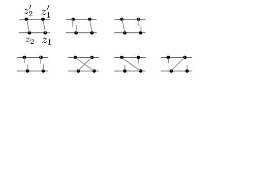
We can now turn to the joint PDF $q(X_{1},X_{2},X^{\prime}_{1},X^{\prime}_{2})$ of (i) the maximum (variable $X_{1}$) and second maximum ($X_{2}$) at time $t$ (ii) the maximum (variable $X^{\prime}_{1}$) and second maximum ($X^{\prime}_{2}$) at time $t^{\prime}$. There are several possible cases, depending on which particle realizes the maximum or second maximum at each of the two times. We can indicate them schematically as

$$(X_{1},X^{\prime}_{1},X_{2},X^{\prime}_{2})=(i,i,j,j)\quad,\quad j\neq i$$ (271)

$$(X_{1},X^{\prime}_{1},X_{2},X^{\prime}_{2})=(i,i,j,j^{\prime})\quad,\quad j\neq i,j\neq j^{\prime},j^{\prime}\neq i$$ (272)

$$(X_{1},X^{\prime}_{1},X_{2},X^{\prime}_{2})=(i,i^{\prime},j,j)\quad,\quad i\neq j,i^{\prime}\neq i,j\neq i^{\prime}$$ (273)

$$(X_{1},X^{\prime}_{1},X_{2},X^{\prime}_{2})=(i,i^{\prime},j,j^{\prime})\quad,\quad i\neq i^{\prime},j\neq j^{\prime},i\neq j,i^{\prime}\neq j^{\prime}$$ (274)

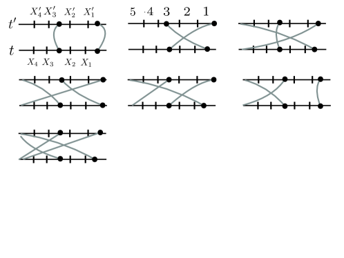
Note that in the last case $i=j^{\prime}$ is possible and so is $i^{\prime}=j$ and so is both at the same time. So in total there are seven terms which read (the terms are illustrated in Fig. 6)

$$q(X_{1},X_{2},X^{\prime}_{1},X^{\prime}_{2})=\sum_{i\neq j}p_{i}(X_{1},X^{\prime}_{1})p_{j}(X_{2},X^{\prime}_{2})\prod_{r\neq i,j}P_{r}(x<X_{2},x^{\prime}<X^{\prime}_{2})$$ (275)

$$+\sum_{i\neq j,i\neq j^{\prime},j\neq j^{\prime}}p_{i}(X_{1},X^{\prime}_{1})p_{j}(X_{2},x^{\prime}<X^{\prime}_{2})p_{j^{\prime}}(x<X_{2},X^{\prime}_{2})\prod_{r\neq i,j,j^{\prime}}P_{r}(x<X_{2},x^{\prime}<X^{\prime}_{2})$$

$$+\sum_{i\neq i^{\prime},i\neq j,i^{\prime}\neq j}p_{i}(X_{1},x^{\prime}<X^{\prime}_{2})p_{i^{\prime}}(x<X_{2},X^{\prime}_{1})p_{j}(X_{2},X^{\prime}_{2})\prod_{r\neq i,i^{\prime},j}P_{r}(x<X_{2},x^{\prime}<X^{\prime}_{2})$$

$$+\sum_{i,j,i^{\prime},j^{\prime}\text{all distinct}}p_{i}(X_{1},x^{\prime}<X^{\prime}_{2})p_{i^{\prime}}(x<X_{2},X^{\prime}_{1})p_{j}(X_{2},x^{\prime}<X^{\prime}_{2})p_{j^{\prime}}(x<X_{2},X^{\prime}_{2})\prod_{r\neq i,i^{\prime},j,j^{\prime}}P_{r}(x<X_{2},x^{\prime}<X^{\prime}_{2})$$

$$+\sum_{i\neq j}p_{i}(X_{1},X^{\prime}_{2})p_{j}(X_{2},X^{\prime}_{1})\prod_{r\neq i,j}P_{r}(x<X_{2},x^{\prime}<X^{\prime}_{2})$$

$$+\sum_{i\neq i^{\prime},i\neq j,i^{\prime}\neq j}p_{i}(X_{1},X^{\prime}_{2})p_{i^{\prime}}(x<X_{2},X^{\prime}_{1})p_{j^{\prime}}(X_{2},x^{\prime}<X^{\prime}_{2})\prod_{r\neq i,j,j^{\prime}}P_{r}(x<X_{2},x^{\prime}<X^{\prime}_{2})$$

$$+\sum_{i\neq i^{\prime},i\neq j,i^{\prime}\neq j}p_{i}(X_{1},x^{\prime}<X^{\prime}_{2})p_{i^{\prime}}(X_{2},X^{\prime}_{1})p_{j^{\prime}}(x<X_{2},X_{2}^{\prime})\prod_{r\neq i,j,j^{\prime}}P_{r}(x<X_{2},x^{\prime}<X^{\prime}_{2})$$

We can now estimate each term in the large $N$ limit (for identical particles) introducing the variables $z_{1},z_{2},z^{\prime}_{1},z^{\prime}_{2}$, and using the same rules for the asymptotics of the various PDF, CDF and mixed PDF/CDF as explained above. One obtains, for each term of (275) in the same order (we abusively denote by the same letter $q$ the two joint PDF)

$$q(X_{1},X_{2},X^{\prime}_{1},X^{\prime}_{2})dX_{1}dX_{2}dX^{\prime}_{1}dX^{\prime}_{2}\simeq q(z_{1},z_{2},z^{\prime}_{1},z^{\prime}_{2})dz_{1}dz_{2}dz^{\prime}_{1}dz^{\prime}_{2}$$ (276)

$$q(z_{1},z_{2},z^{\prime}_{1},z^{\prime}_{2})=\bigg{(}\partial_{z_{1}}\partial_{z^{\prime}_{1}}\Phi(z_{1},z^{\prime}_{1})\partial_{z_{2}}\partial_{z^{\prime}_{2}}\Phi(z_{2},z^{\prime}_{2})-\partial_{z_{1}}\partial_{z^{\prime}_{1}}\Phi(z_{1},z^{\prime}_{1})\partial_{z_{2}}\Phi(z_{2},z^{\prime}_{2})\partial_{z^{\prime}_{2}}\Phi(z_{2},z^{\prime}_{2})$$ (277)

$$-\partial_{z_{1}}\Phi(z_{1},z^{\prime}_{2})\partial_{z^{\prime}_{1}}\Phi(z_{2},z^{\prime}_{1})\partial_{z_{2}}\partial_{z^{\prime}_{2}}\Phi(z_{2},z^{\prime}_{2})+\partial_{z_{1}}\Phi(z_{1},z^{\prime}_{2})\partial_{z^{\prime}_{1}}\Phi(z_{2},z^{\prime}_{1})\partial_{z_{2}}\Phi(z_{2},z^{\prime}_{2})\partial_{z^{\prime}_{2}}\Phi(z_{2},z^{\prime}_{2})$$

$$+\partial_{z_{1}}\partial_{z^{\prime}_{2}}\Phi(z_{1},z^{\prime}_{2})\partial_{z_{2}}\partial_{z^{\prime}_{1}}\Phi(z_{2},z^{\prime}_{1})-\partial_{z_{1}}\partial_{z^{\prime}_{2}}\Phi(z_{1},z^{\prime}_{2})\partial_{z^{\prime}_{1}}\Phi(z_{2},z^{\prime}_{1})\partial_{z_{2}}\Phi(z_{2},z^{\prime}_{2})$$

$$-\partial_{z_{1}}\Phi(z_{1},z^{\prime}_{2})\partial_{z_{2}}\partial_{z^{\prime}_{1}}\Phi(z_{2},z^{\prime}_{1})\partial_{z^{\prime}_{2}}\Phi(z_{2},z^{\prime}_{2})\bigg{)}e^{\Phi(z_{2},z^{\prime}_{2})}$$

where for clarity we have made the time argument implicit, i.e. $\Phi(z,z^{\prime})\equiv\Phi(z,z^{\prime},\tau)$. Recall that each term gives the respective probabilities of how the particle realizing the maximum and second maximum change from time $t$ to time $t^{\prime}$. For instance the first term corresponds to events where both the rightmost particle and the second rightmost at $t$ have remained so at $t^{\prime}$, and so on.

It turns out that the rather bulky expression (276),(277) is a total derivative, i.e. one can check that, for $z_{1}>z_{2}$, $z^{\prime}_{1}>z^{\prime}_{2}$,

$$q(z_{1},z_{2},z^{\prime}_{1},z^{\prime}_{2})=\partial_{z_{1}}\partial_{z^{\prime}_{1}}\partial_{z_{2}}\partial_{z^{\prime}_{2}}(-\Phi(z_{1},z^{\prime}_{1})+\Phi(z_{1},z^{\prime}_{2})\Phi(z_{2},z^{\prime}_{1}))e^{\Phi(z_{2},z^{\prime}_{2})}$$ (278)

which is the result (106) displayed in the text, where it is also derived by a different method using counting statistics.

Appendix E Multi-time, multi-space counting statistics

One can generalize the arguments in Section 6.2. Let us illustrate for $n=3$ times and an arbitrary number of points $k$, $k^{\prime}$ and $k^{\prime\prime}$. Here we denote $t^{\prime}-t=t\frac{\tau}{\log N}$ and $t^{\prime\prime}-t^{\prime}=t\frac{\tau^{\prime}}{\log N}$, with $\tau,\tau^{\prime}=O(1)$. Consider the three sequences of points $\{X_{j}\}_{j=1,\dots,k}$, $\{X^{\prime}_{j^{\prime}}\}_{j^{\prime}=1,\dots,k^{\prime}}$, $\{X^{\prime\prime}_{j^{\prime\prime}}\}_{j^{\prime\prime}=1,\dots,k^{\prime\prime}}$, each being in decreasing order. For each time the real axis is the union of $k+1$ (and then $k^{\prime}+1$ and $k^{\prime\prime}+1$) contiguous intervals, e.g. at time $t$ these are $[X_{j},X_{j-1}]$, $j=1,k+1$ with by convention $X_{0}=+\infty$ and $X_{k+1}=-\infty$, and similarly for $t^{\prime}$ and $t^{\prime\prime}$. Let $n_{j,j^{\prime},j^{\prime\prime}}$, for $j=1,\dots,k+1$, $j^{\prime}=1,\dots,k^{\prime}+1$, $j^{\prime\prime}=1,\dots,k^{\prime\prime}+1$, be the numbers of particles which are in $[X_{j},X_{j-1}]$ at $t$ and in $[X^{\prime}_{j^{\prime}},X^{\prime}_{j^{\prime}-1}]$ at $t^{\prime}$ and in $[X^{\prime\prime}_{j^{\prime\prime}},X^{\prime\prime}_{j^{\prime\prime}-1}]$ at $t^{\prime\prime}$. The set of these numbers obey a multinomial distribution. In the large $N$ limit, in the (multi-time) edge regime, defined such that the corresponding variables $z_{j},z^{\prime}_{j^{\prime}},z^{\prime\prime}_{j^{\prime\prime}}$ are all of order $O(1)$, all of these numbers are of order $O(1)$ with the exception of $n_{k+1,k^{\prime}+1,k^{\prime\prime}+1}\simeq N$. Then this reduced set of numbers are independent Poisson variables, each with mean parameter $\lambda_{j,j^{\prime},j^{\prime\prime}}$. These parameters can be related to the functions defined in this paper as follows

$$\lambda_{j,j^{\prime},j^{\prime\prime}}=\langle(\theta_{x>X_{j}}-\theta_{x>X_{j-1}})(\theta_{x^{\prime}>X^{\prime}_{j^{\prime}}}-\theta_{x^{\prime}>X^{\prime}_{j^{\prime}-1}})(\theta_{x^{\prime\prime}>X^{\prime\prime\prime}_{j^{\prime\prime}}}-\theta_{x^{\prime\prime}>X^{\prime\prime\prime}_{j^{\prime\prime}-1}})\rangle$$ (279)

$$\simeq\sum_{\ell=0,1}\sum_{\ell^{\prime}=0,1}\sum_{\ell^{\prime\prime}=0,1}(-1)^{\ell+\ell^{\prime}+\ell^{\prime\prime}}g_{3}(z_{j-\ell},z^{\prime}_{j^{\prime}-\ell^{\prime}},z^{\prime\prime}_{j^{\prime\prime}-\ell^{\prime\prime}};\tau,\tau^{\prime})$$ (280)

where $g_{3}$ was defined in (34). We recall the convention $z_{0}=z^{\prime}_{0}=z^{\prime\prime}_{0}=+\infty$ and $z_{k+1}=z^{\prime}_{k^{\prime}+1}=z^{\prime\prime}_{k^{\prime\prime}+1}=-\infty$. As mentionned in Section 3, $g_{3}$ vanishes when any of the $z$ argument is taken to $+\infty$, and reduces to $g_{2}=g$ when any of the $z$ argument is taken to $-\infty$, more precisely one has $g_{3}(-\infty,z^{\prime},z^{\prime\prime},\tau,\tau^{\prime})=g(z^{\prime},z^{\prime\prime},\tau^{\prime})$, $g_{3}(z,-\infty,z^{\prime\prime},\tau,\tau^{\prime})=g(z,z^{\prime\prime},\tau+\tau^{\prime})$, $g_{3}(z,z^{\prime},-\infty,\tau,\tau^{\prime})=g(z,z^{\prime},\tau)$, and similarly for $g_{2}=g$ which reduces to $g_{1}(z)=e^{-z}$. One can check that the sum of all the $\lambda_{j,j^{\prime},j^{\prime\prime}}$ (over all indices, not including $(j,j^{\prime},j^{\prime\prime})=(k+1,k^{\prime}+1,k^{\prime\prime}+1)$) equals $\Phi(z_{k},z^{\prime}_{k^{\prime}},z^{\prime\prime}_{k^{\prime\prime}};\tau,\tau^{\prime})$, yielding the normalization factor $e^{-\Phi(z_{k},z^{\prime}_{k^{\prime}},z^{\prime\prime}_{k^{\prime\prime}};\tau,\tau^{\prime})}$ for the multiple independent Poisson distribution of the $n_{j,j^{\prime},j^{\prime\prime}}$.

Two times, three first maxima. Let us first return to the case of $2$ times. The probability that the maximum is in $[X_{1},+\infty[$ and the second maximum is in $]-\infty,X_{2}]$ at $t$, and the maximum is in $[X^{\prime}_{1},+\infty[$ and the second maximum is in $]-\infty,X^{\prime}_{2}]$ at $t^{\prime}$ was given in (120), and reads, translated in the present notations

$$(\lambda_{11}+\lambda_{13}\lambda_{31})e^{-\Phi(z_{2},z^{\prime}_{2};\tau)}$$ (281)

which is a sum over the two permutations of 2 elements. Upon taking the derivatives $\partial_{z_{1}}\partial_{z_{2}}\partial_{z^{\prime}_{1}}\partial_{z^{\prime}_{2}}$ yields the two time joint PDF of the maximum and second maximum.

Figure 7: Interpretation of the different terms in (283) in the order in which they appear, left to right and top to bottom. Only the maximum and second maximum and their trajectories are shown at each time.

This can be generalized. For instance consider $n=2$ and $k=k^{\prime}=4$ and the following joint probability

$${\cal P}={\rm Prob}(X^{(1)}(t)>X_{1},X^{(2)}(t)\in[X_{3},X_{2}],X^{(3)}(t)<X_{4},X^{(1)}(t^{\prime})>X^{\prime}_{1},X^{(2)}(t^{\prime})\in[X^{\prime}_{3},X^{\prime}_{2}],X^{(3)}(t^{\prime})<X^{\prime}_{4})$$ (282)

From ${\cal P}$ one can obtain by differentiation the two time joint PDF of the maximum, second maximum and third maximum. The various cases are shown in Fig. (7) and one obtains

$${\cal P}\simeq(\lambda_{11}\lambda_{33}+\lambda_{13}\lambda_{31}+\lambda_{15}\lambda_{51}\lambda_{33}+\lambda_{13}\lambda_{35}\lambda_{51}+\lambda_{15}\lambda_{53}\lambda_{31}+\lambda_{11}\lambda_{35}\lambda_{53}+\lambda_{15}\lambda_{51}\lambda_{35}\lambda_{53})e^{-\Phi(z_{3},z^{\prime}_{3},\tau)}$$ (283)

which, apart from the last term, is a sum over the six permutations of three elements. Note that the intervals $[X_{2},X_{1}]$ and $[X_{4},X_{3}]$ remain empty. The two time 3-order statistics PDF is obtained as (in the $z$ variables)

$$q(z_{1},z_{2},z_{3},z^{\prime}_{1},z^{\prime}_{2},z^{\prime}_{3})=\partial_{z_{1}}\partial_{z_{2}}\partial_{z_{3}}\partial_{z^{\prime}_{1}}\partial_{z^{\prime}_{2}}\partial_{z^{\prime}_{3}}{\cal P}$$ (284)

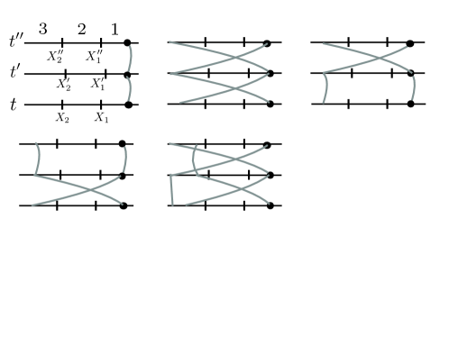
Three times, two first maxima. One can also obtain the three time joint PDF of the maximum and second maximum. From Fig. 8 we see that, for $z_{1}>z_{2}$, $z^{\prime}_{1}>z^{\prime}_{2}$, $z^{\prime\prime}_{1}>z^{\prime\prime}_{2}$,

$$q(z_{1},z_{2},z^{\prime}_{1},z^{\prime}_{2},z^{\prime\prime}_{1},z^{\prime\prime}_{2})=$$ (285)

$$\partial_{z_{1}}\partial_{z_{2}}\partial_{z^{\prime}_{1}}\partial_{z^{\prime}_{2}}\partial_{z^{\prime\prime}_{1}}\partial_{z^{\prime\prime}_{2}}\big{(}(\lambda_{111}+\lambda_{131}\lambda_{313}+\lambda_{113}\lambda_{331}+\lambda_{133}\lambda_{311}+\lambda_{133}\lambda_{331}\lambda_{313})e^{-\Phi(z_{2},z^{\prime}_{2},z^{\prime\prime}_{2};\tau,\tau^{\prime})}\big{)}$$

which has $2!^{2}$ terms (two successive permutations of 2 elements). To be specific we give

$$\lambda_{111}=g_{3}(z_{1},z^{\prime}_{1},z^{\prime\prime}_{1};\tau,\tau^{\prime})$$ (286)

$$\lambda_{113}=g(z_{1},z^{\prime}_{1},\tau)-g_{3}(z_{1},z^{\prime}_{1},z^{\prime\prime}_{2};\tau,\tau^{\prime})$$ (287)

$$\lambda_{331}=e^{-z^{\prime\prime}_{1}}-g_{2}(z_{2},z^{\prime\prime}_{1};\tau+\tau^{\prime})-g(z^{\prime}_{2},z^{\prime\prime}_{1},\tau^{\prime})+g_{3}(z_{2},z^{\prime}_{2},z^{\prime\prime}_{1};\tau,\tau^{\prime})$$ (288)

$$\lambda_{133}=e^{-z_{1}}-g(z_{1},z^{\prime}_{2};\tau)-g(z_{1},z^{\prime\prime}_{2};\tau+\tau^{\prime})+g_{3}(z_{1},z^{\prime}_{2},z^{\prime\prime}_{2};\tau,\tau^{\prime})$$ (289)

$$\lambda_{311}=g(z^{\prime}_{1},z^{\prime\prime}_{1},\tau^{\prime})-g_{3}(z_{2},z^{\prime}_{1},z^{\prime\prime}_{1};\tau,\tau^{\prime})$$ (290)

$$\lambda_{131}=g(z_{1},z^{\prime\prime}_{1},\tau+\tau^{\prime})-g_{3}(z_{1},z^{\prime}_{2},z^{\prime\prime}_{1};\tau,\tau^{\prime})$$ (291)

$$\lambda_{313}=e^{-z^{\prime}_{1}}-g(z_{2},z^{\prime}_{1};\tau)-g(z^{\prime}_{1},z^{\prime\prime}_{2};\tau^{\prime})+g_{3}(z_{2},z^{\prime}_{1},z^{\prime\prime}_{2};\tau,\tau^{\prime})$$ (292)

Figure 8: Interpretation of the different terms in (285) in the order in which they appear, left to right and top to bottom. Only the maximum and its trajectory is shown at each time.

Appendix F Continuum time observables: calculations

F.1   First passage time

Let us recall the following. Let $B(t)$ the standard Brownian motion (i.e. with $B(0)=0$) and $W(t)=\sqrt{D}B(t)+\mu$ a Brownian with drift $\mu$ and diffusion coefficient $D$. Let us denote $T^{\mu,D}_{z}$ the first passage time of $W(t)$ at level $z$. For $z>0$ the PDF of $T=T_{z}^{\mu,D}$ is

$$p_{z}(T)=\frac{z}{\sqrt{2\pi D}T^{3/2}}e^{-\frac{(z-\mu T)^{2}}{2DT}}+\delta_{+\infty}(T)(1-e^{2\mu z/D})\theta(-\mu)$$ (293)

One has upon integration

$${\rm Prob}(T_{z}^{\mu,D}>t)=\frac{1}{2}({\rm erfc}(\frac{\mu t-z}{\sqrt{2Dt}})-e^{2\mu z/D}{\rm erfc}(\frac{\mu t+z}{\sqrt{2Dt}}))$$ (294)

For $\mu=0$ it simplifies into

$${\rm Prob}(T_{z}^{0,D}>t)={\rm erf}(\frac{z}{\sqrt{2Dt}})$$ (295)

Eq. (294) is also the probability that a Brownian survives up to time $t$ in presence of an absorbing wall at $x=z$ and can thus also be obtained from the image method. Indeed one has, denoting $x$ the position of the Brownian at time $t$,

$${\rm Prob}(T_{z}^{\mu,D}>t)=\int_{-\infty}^{z}dx(\frac{e^{-(x-\mu t)^{2}/(2Dt)}}{\sqrt{2\pi Dt}}-e^{2\mu z/D}\frac{e^{-(x-2z-\mu t)^{2}/(2Dt)}}{\sqrt{2\pi Dt}})$$ (296)

which upon integration recovers (294).

F.2   Probability that the maximum remains below a straight line

Let us consider the following observable for the maximum process $X(t)=X^{(1)}(t)$ of $N$ standard Brownian motions started at the origin

$${\rm Prob}(X(t)<X_{1}+v(t-t_{1})~{},~{}\forall t\in[t_{1},t_{2}])={\rm Prob}(x(t)<X_{1}+v(t-t_{1})~{},~{}\forall t\in[t_{1},t_{2}])^{N}$$ (297)

Now one has

$${\rm Prob}(x(t)<X_{1}+v(t-t_{1})~{},~{}\forall t\in[t_{1},t_{2}])=\int_{-\infty}^{X_{1}}dx_{1}\frac{e^{-x_{1}^{2}/(2t_{1})}}{\sqrt{2\pi t_{1}}}{\rm Prob}(T^{-v}_{X_{1}-x_{1}}>t_{2}-t_{1})$$ (298)

where here we must set $D=1$. Indeed, asking that a standard Brownian motion starting at $x_{1}$ at time $t_{1}$, remains below $X_{1}+v(t-t_{1})$ until $t_{2}$ is equivalent to asking that a standard drifted Brownian of drift $-v$ remains below $X_{1}$ until $t_{2}$, which is also equivalent to asking that the first passage time at level $X_{1}$ of a drifted Brownian of drift $-v$ started at $x_{1}$ at time $t_{1}$ is larger than $t_{2}-t_{1}$. Using (294) one obtains

$${\cal P}:={\rm Prob}(x(t)<X_{1}+v(t-t_{1})~{},~{}\forall t\in[t_{1},t_{2}])$$ (299)

$$=\int_{-\infty}^{X_{1}}dx_{1}\frac{e^{-x_{1}^{2}/(2t_{1})}}{\sqrt{2\pi t_{1}}}\frac{1}{2}\bigg{(}{\rm erfc}(\frac{-v(t_{2}-t_{1})-(X_{1}-x_{1})}{\sqrt{2(t_{2}-t_{1})}})-e^{-2(X_{1}-x_{1})v}{\rm erfc}(\frac{-v(t_{2}-t_{1})+(X_{1}-x_{1})}{\sqrt{2(t_{2}-t_{1})}}\bigg{)}$$

We will now scale $X$ near the edge, and scale the time window as well, i.e. choose

$$X_{1}=\sqrt{2t_{1}\log N}(1+\frac{z_{1}+c_{N}}{2\log N})\quad,\quad\frac{t_{2}-t_{1}}{t_{1}}=\frac{\tau_{2,1}}{\log N}$$ (300)

and we will need to scale the slope $v$ as

$$v=w\sqrt{\frac{\log N}{2t_{1}}}\quad,\quad w=O(1)$$ (301)

In that region ${\cal P}$ is close to unity, with $1-{\cal P}=O(1/N)$ and

$${\rm Prob}(X(t)<X_{1}+v(t-t_{1})~{},~{}\forall t\in[t_{1},t_{2}])={\cal P}^{N}\simeq e^{-N(1-{\cal P})}$$ (302)

Using that the edge coordinates satisfy

$$Np_{t_{1}}(x_{1})dx_{1}=e^{-y_{1}}dy_{1}\quad,\quad X_{1}-x_{1}=\frac{\sqrt{2t_{1}}}{2\sqrt{\log N}}(z_{1}-y_{1})$$ (303)

We can write

$$N(1-{\cal P})=N\int_{-\infty}^{+\infty}dx_{1}\frac{e^{-x_{1}^{2}/(2t_{1})}}{\sqrt{2\pi t_{1}}}$$ (304)

$$\times\bigg{(}1-\theta(X_{1}-x_{1})\frac{1}{2}\big{(}{\rm erfc}(\frac{-v(t_{2}-t_{1})-(X_{1}-x_{1})}{\sqrt{2(t_{2}-t_{1})}})-e^{-2(X_{1}-x_{1})v}{\rm erfc}(\frac{-v(t_{2}-t_{1})+(X_{1}-x_{1})}{\sqrt{2(t_{2}-t_{1})}}\big{)}\bigg{)}$$

$$\simeq\int dy_{1}e^{-y_{1}}(1-\theta(z_{1}-y_{1})\frac{1}{2}\big{(}{\rm erfc}(\frac{-w\tau_{2,1}-(z_{1}-y_{1})}{2\sqrt{\tau_{2,1}}})-e^{-(z_{1}-y_{1})w}{\rm erfc}(\frac{-w\tau_{2,1}+(z_{1}-y_{1})}{2\sqrt{\tau_{2,1}}})\big{)}\bigg{)}$$

$$=\int dye^{-y_{1}}(1-\theta(z_{1}-y_{1}){\rm Prob}({\sf T}^{-w}_{z_{1}-y_{1}}>\tau_{2,1}))=e^{-z_{1}}\int dye^{y}(1-\theta(y){\rm Prob}({\sf T}^{-w}_{y}>\tau_{2,1}))$$ (305)

where in the last line we have set $y_{1}=z_{1}-y$ and where ${\sf T}^{-w}_{z}=T^{-w,D=2}_{z}$ is the first passage time for a Brownian with drift $-w$ and diffusion coefficient $D=2$, with

$${\rm Prob}({\sf T}^{-w}_{y}>\tau)=\frac{1}{2}\big{(}{\rm erfc}(\frac{-w\tau-y}{2\sqrt{\tau}})-e^{-yw}{\rm erfc}(\frac{-w\tau+y}{2\sqrt{\tau}})\big{)}\bigg{)}$$ (306)

In summary we find that

$${\rm Prob}(X(t)<X_{1}+v(t-t_{1})~{},~{}\forall t\in[t_{1},t_{2}])~{}\simeq~{}e^{-e^{-z_{1}}\Psi_{w}(\tau_{2,1})}$$ (307)

where

$$\Psi_{w}(\tau)=\int dye^{y}(1-\theta(y){\rm Prob}({\sf T}^{-w}_{y}>\tau))=1-\int_{y>0}dy\,e^{y}\,{\rm Prob}({\sf T}^{-w}_{y}<\tau)$$ (308)

An explicit calculation and one finds, for $w\neq 1$

$$\Psi_{w}(\tau)=\frac{2-w}{1-w}\left(-\frac{1}{2}e^{\tau-\tau w}\text{erfc}\left(\frac{1}{2}\sqrt{\tau}(w-2)\right)+\left(\frac{1}{w-2}+\frac{1}{2}\right)\text{erfc}\left(\frac{\sqrt{\tau}w}{2}\right)+1\right)$$ (309)

with $\Psi_{w}(0)=1$. For $w=1$ it gives (157) in the text, and for $w=0$ one has

$$\Psi_{0}(\tau)=e^{\tau}\left(\text{erfc}\left(\sqrt{\tau}\right)-2\right)+2$$ (310)

Now under the rescaling described here and the definition of $z(\tau)$ in the text one finds that

$${\rm Prob}(X(t)<X_{1}+v(t-t_{1})~{},~{}\forall t\in[t_{1},t_{2}])\simeq{\rm Prob}(z(\tau)+\tau<z_{1}+w\tau)$$ (311)

which shows the result (156) conjectured in the text.

F.3   Running maximum and arrival time of the first particle: one time

Here we derive the one-time distributions by a more detailed calculation. For the standard Brownian motion, we see from (295) that Eq. (158) becomes

$${\rm Prob}(r(t_{1})<R_{1})={\rm Prob}(T_{R_{1}}>t_{1})={\cal P}_{1}={\rm erf}(\frac{R_{1}}{\sqrt{2t_{1}}})$$ (312)

This can be either interpreted as the CDF for the running maximum at fixed $t_{1}$ or for the ”CDF” of the first passage time at fixed $R_{1}$. Similarly for $N$ Brownian one has

$${\rm Prob}(R(t_{1})<R_{1})={\rm Prob}(T^{\min}_{R_{1}}>t_{1})$$ (313)

can be interpreted either as the CDF of $R(t_{1})=\max_{i}r_{i}(t_{1})$ at fixed $t_{1}$, or the ”CDF” of the arrival time of the first particle, $T^{\min}_{R_{1}}=\min_{i}T^{(i)}_{R_{1}}$ at fixed $R_{1}$. At large $N$ (313) is estimated as

$$\simeq e^{-N(1-{\cal P}_{1})}=e^{-N(1-{\rm erf}(\frac{R_{1}}{\sqrt{2t_{1}}}))}\simeq e^{-N\frac{\sqrt{2t_{1}}}{\sqrt{\pi}R_{1}}e^{-\frac{R_{1}^{2}}{2t_{1}}}}=e^{-e^{-z}}$$ (314)

where

$$\frac{R_{1}^{2}}{2t_{1}}=\log N+z-\log\frac{\sqrt{\pi}R_{1}}{\sqrt{2t_{1}}}\simeq\log N+z+c^{\prime}_{N}\quad,\quad c^{\prime}_{N}=-\frac{1}{2}\log(\pi\log N)=c_{N}+\log 2$$ (315)

If we are interested in the running maximum at fixed $t_{1}$ we obtain from this estimate

$$R(t_{1})=R_{1}=\sqrt{2t_{1}\log N}(1+\frac{z_{1}+c_{N}}{2\log N}))\quad,\quad z_{1}=z+\log 2$$ (316)

in agreement with the text, where $z$ is Gumbel distributed (by definition from (314)), and the shift of $\log 2$ agrees with the one obtained in (165). On the other hand, if one is interested in the arrival time of the first particle one obtains, from the same estimate

$$T^{\rm\min}_{R_{1}}=t_{1}=\frac{R_{1}^{2}}{2\log N}(1-\frac{z+c^{\prime}_{N}}{\log N}))$$ (317)

where $z$ is Gumbel distributed. One may ask why is the arrival time of the first particle also distributed with (minus) Gumbel, since the distribution of the first passage time is very different from a Gaussian, see (293). To see that immediately one can consider that $\min_{i}T^{(i)}_{R}=1/(\max_{i}U_{i})$ where $U=1/T_{R}$ has a distribution with an exponential tail which clearly belongs to Gumbel class.

F.4   Running maximum and arrival time of the first particle: two time

We give here more details of the calculation of the two-time joint CDF of the running maximum depicted in the text. Let us start from the exact expression for ${\cal P}$ in (169). In the large $N$ limit, with the scaling (170), using similar estimates as in Appendix A, we obtain

$$N(1-{\cal P})=N\int dx_{1}\int dx_{2}\bigg{(}\frac{e^{-\frac{x_{1}^{2}}{2t_{1}}}}{\sqrt{2\pi t_{1}}}\frac{e^{-\frac{(x_{2}-x_{1})^{2}}{2(t_{2}-t_{1})}}}{\sqrt{2\pi(t_{2}-t_{1})}}$$ (318)

$$\times\bigg{(}1-\theta(R_{1}-x_{1})\theta(R_{2}-x_{2})(1-e^{-\frac{2R_{1}(R_{1}-x_{1})}{t_{1}}})(1-e^{-\frac{2(R_{2}-x_{1})(R_{2}-x_{2})}{t_{2}-t_{1}}})\bigg{)}$$

$$\simeq\int dy_{1}\int dy_{2}\frac{e^{-\frac{(y_{2}-y_{1}+\tau)^{2}}{4\tau}}}{\sqrt{4\pi\tau}}(e^{-y_{1}}-\theta(z_{1}-y_{1})\theta(z_{2}-y_{2})(e^{-y_{1}}-e^{-(2z_{1}-y_{1})})(1-e^{-\frac{(z_{2}+\tau-y_{1})(z_{2}-y_{2})}{\tau}})$$

where we have changed variables denoting $x_{i}=\sqrt{2t_{i}\log N}(1+\frac{y_{i}+c_{N}}{2\log N})$. As for the functions $\Phi$ we can give some interpretation to this formula in terms of the Brownian motion with unit negative drift and diffusion coefficient $D=2$, with however an important difference. The factor $(e^{-y_{1}}-e^{-(2z_{1}-y_{1})})\theta(z_{1}-y_{1})$ is the stationary measure in the presence of an absorbing wall at $z_{1}$. The other factor can be written as

$$\theta(z_{2}-y_{2})\left(\frac{e^{-\frac{(y_{2}-y_{1}+\tau)^{2}}{4\tau}}}{\sqrt{4\pi\tau}}-\frac{e^{-\frac{(y_{2}-(2(z_{2}+\tau)-y_{1})+\tau)^{2}}{4\tau}}}{\sqrt{4\pi\tau}}\right)$$ (319)

which vanishes at $y_{2}=z_{2}$ but is not exactly the propagator in presence of a fixed absorbing wall, since the wall is effectively moving. Performing the change of variable $y_{1}\to z_{1}-y_{1}$ and $y_{2}\to z_{2}-y_{2}$ in the last line of (318) one obtains

$${\rm Prob}(R(t_{1})<R_{1},R(t_{2})<R_{2})\simeq e^{-N(1-{\cal P})}\simeq e^{-e^{-z_{1}}\gamma_{\tau}(z_{21})}$$ (320)

with the function $\gamma_{\tau}(z)$ displayed in (172) in the text. To obtain the explicit expression (173) one splits the integral into $y_{1}>0$ and $y_{1}<0$ and use that $\int_{y_{1}<0}\int dy_{2}e^{y_{1}}G(z-y_{2,1},\tau)=1$. The part $y_{1}>0,y_{2}<0$ is found to equal $\phi_{\tau}(z)-1$. The remaining part $y_{1}>0,y_{2}>0$, which is positive, can be integrated explicitly.

F.5   Multi-time CDF for the running maximum

The two-time calculation of the previous section can easily be extended to any number of times $n$. Here we just give the result. One finds, under the scaling (170) and $t_{j}-t_{j-1}=t_{1}\tau_{j,j-1}/\log N$

$${\rm Prob}(R(t_{1})<R_{1},\dots,R(t_{n})<R_{n})={\rm Prob}(T^{\rm min}_{R_{1}}>t_{1},\dots,T^{\rm min}_{R_{n}}>t_{n})\simeq e^{-\Gamma(z_{1},\dots,z_{n};\tau_{2,1},\dots,\tau_{n,n-1})}$$ (321)

where

$$\Gamma(z_{1},\dots,z_{n};\tau_{2,1},\dots,\tau_{n,n-1})=\int dy_{1}\int dy_{2}\dots dy_{n}\,e^{-y_{1}}G(y_{2,1},\tau_{2,1})\dots G(y_{n,n-1},\tau_{n,n-1})$$ (322)

$$\times(1-\prod_{i=1}^{n}\theta(z_{i}-y_{i})(1-e^{-2(z_{1}-y_{1})})(1-e^{-\frac{(z_{2}+\tau-y_{1})(z_{2}-y_{2})}{\tau}})\dots(1-e^{-\frac{(z_{n}+\tau_{n,n-1}-y_{n})(z_{n}-y_{n})}{\tau_{n,n-1}}})$$

Similarly, the result (321), (322) can be read as a result for the multi-time joint ”CDF” of the arrival times $T^{\rm min}_{R_{i}}$ of the first particle at $R_{i}$, which allows to obtain the joint distribution of $z_{1}$, and of the scaled delay times $\tau_{2,1},\dots,\tau_{n,n-1}$, defined as in (201) in the text.

References

- [1] B.V. Gnedenko, Sur la distribution limite du terme maximum d’une série aléatoire. Ann. Math. 44, 423-453, (1943).
- [2] E.J. Gumbel, Statistics of Extremes, Dover, (1958).
- [3] J. Galambos, The Asymptotic Theory of Extreme Order Statistics, R.E. Krieger Publishing. Co., Malabar, Florida (1987).
- [4] H.N. Nagaraja, H.A. David, Order statistics, (third ed.), Wiley, New Jersey (2003).
- [5] G. Barraquand, I. Corwin, Random-walk in beta-distributed random environment, arXiv:1503.04117, Probab. Theory Rel. Fields, 167(3):1057-1116, (2017).
- [6] P. Le Doussal, T. Thiery, Diffusion in time-dependent random media and the Kardar-Parisi-Zhang equation, arXiv:1705.05159, Phys. Rev. E 96, 010102 (2017).
- [7] G. Barraquand and M. Rychnovsky. Large deviations for sticky Brownian motions. arXiv:1905.10280, (2019).
- [8] G. Barraquand, P. Le Doussal, Moderate deviations for diffusion in time dependent random media, arXiv:1912.11085, J. Phys. A: Math. Theor. 53.21: 215002, (2020).
- [9] J. B. Hass, A. N. Carroll-Godfrey, E. I. Corwin, I. Z. Corwin, Anomalous Fluctuations of Extremes in Many-Particle Diffusion, arXiv:2205.02265, Phys. Rev. E 107, L02210 (2023).
- [10] A. Krajenbrink, P. Le Doussal, The crossover from the Macroscopic Fluctuation Theory to the Kardar-Parisi-Zhang equation controls the large deviations beyond Einstein’s diffusion, arXiv:2204.04720, Phys. Rev. E, 107(1):014137 (2023).
- [11] D. Brockington and J. Warren, At the edge of a cloud of Brownian particles. arXiv:2208.11952.
- [12] S. Das, H. Drillick, and S. Parekh, KPZ equation limit of sticky Brownian motion. arXiv:2304.14279.
- [13] J. B. Hass, I. Corwin, E. I. Corwin, First Passage Time for Many Particle Diffusion in Space-Time Random Environments, arXiv:2308.01267.
- [14] E. Corwin and I. Corwin, private communication. See also [9] for numerical tests.
- [15] B. M. Brown, S. I. Resnick, Extreme Values of Independent Stochastic Processes, Journal of Applied Probability, Vol. 14, No. 4, 732-739 (1977).
- [16] L. De Haan, S.I. Resnick, Limit theory for multivariate sample extremes, Zeitschrift fur Wahrscheinlichkeitstheorie und verwandte Gebiete, 40(4), 317-337 (1977).
- [17] J. Husler, R.D. Reiss, maxima of normal random vectors: between independence and complete dependence. Statist. Probab. Letters 7 283-286 (1989).
- [18] G. Hooghiemstra, J. Husler, A note on maxima of bivariate random vectors, Statistics and Probability Letters 31.1, 1-6 (1996).
- [19] see e.g. Section 10.5, p 416 in M. Falk, J. Husler, R-D Reiss, Laws of small numbers: extreme and rare events, Third edition, Birkhauser, Basel (2010).
- [20] L. de Haan, A spectral representation for max-stable processes, The Annals of Probability, 12(4):1194-1204,(1984).
- [21] R. Huser, A. C. Davison, Composite likelihood estimation for the Brown-Resnick process, Biometrika, 100(2), 511-518, (2013).
- [22] E. Bouyé, Multivariate extremes at work for portfolio risk measurement, (2002): 125-144.
- [23] Z. Kabluchko, Extremes of space-time Gaussian processes, Stoch. Proc. Appl. 119, 3962-3980, (2009). Z. Kabluchko, M. Schlather, L de Haan, Stationary max-stable fields associated to negative definite functions, Ann. Probab. 37, 2042-2065, (2009).
- [24] S. Engelke, A. Malinowski, Z. Kabluchko, M. Schlather, Estimation of Husler-Reiss distributions and Brown-Resnick processes, Journal of the Royal Statistical Society Series B: Statistical Methodology, 77(1), 239-265, (2015).
- [25] E. Hashorva, Z. Peng, Z. Weng, Higher-order expansions of distributions of maxima in a Husler-Reiss model. Methodology and Computing in Applied Probability, 18, 181-196, (2016).
- [26] L. Tang, S. Zheng, Z. Tan, Limit theorem on the pointwise maxima of minimum of vector-valued Gaussian processes, Statistics and Probability Letters, 176, 109137, (2021).
- [27] S. N. Majumdar and G. Schehr, in preparation.
- [28] D. S. Dean, S. N. Majumdar and G. Schehr, Effusion of stochastic processes on a line, arXiv:2303.08961, J. Stat. Mech. 063208 (2023).
- [29] O. Bénichou, P.L. Krapivsky, C. Mejia-Monasterio, G. Oshanin, Temporal correlations of the running maximum of a Brownian trajectory, Phys. Rev. Lett., 117(8), 080601 (2016).
- [30] A. L. Hodgkin and R. D. Keynes, J. Physiol. 128, 61 (1955).
- [31] see P. L. Krapivsky, K. Mallick, T. Sadhu, Large deviations in single-file diffusion, Phys. Rev. Lett. 113 078101 (2014) and references therein.
- [32] B. Derrida, Random-energy model: An exactly solvable model of disordered systems, Phys. Rev. B, 24(5), 2613, (1981).
- [33] e.g. for the initial condition considered for and for . Also would be an equally good stationary condition, corresponding to a translation in . This is not surprising since here some details of the initial condition have been erased.