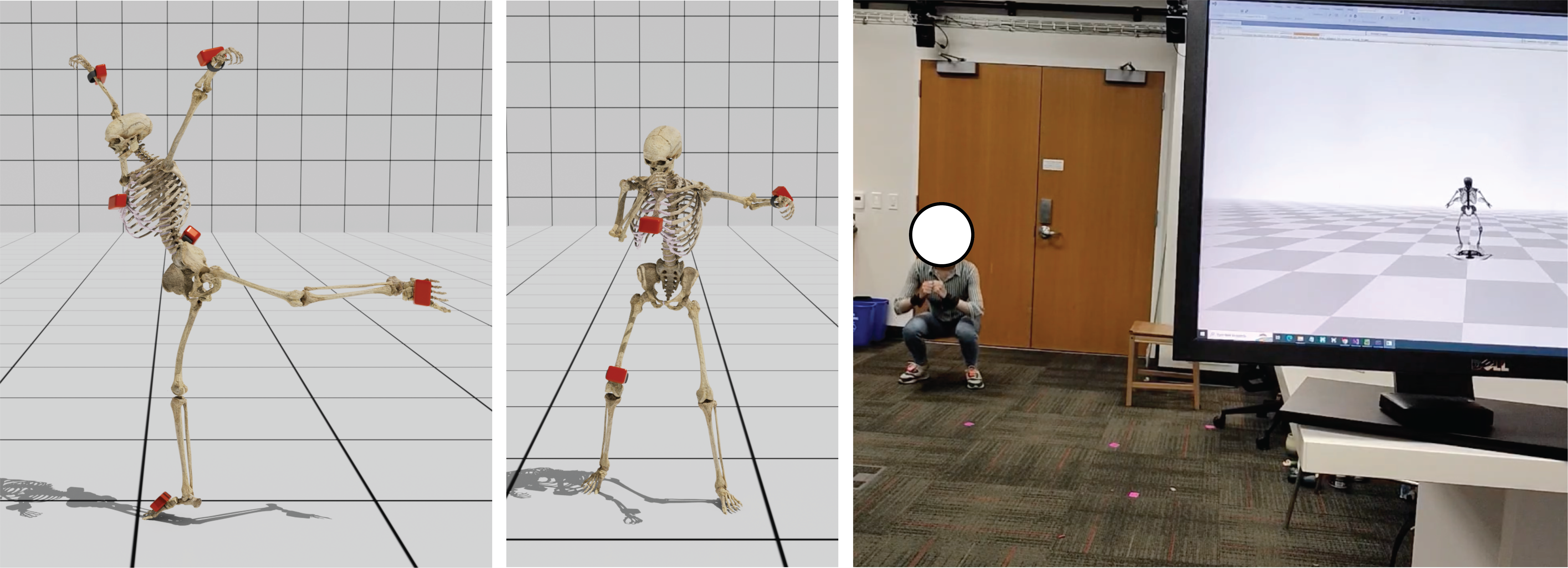
Figure 1. (Left) Human motion reconstructions with sparse and arbitrary IMU configurations. (Right) Live demo where user is wearing 3 IMUs.

Diffusion Inertial Poser: Human Motion Reconstruction from Arbitrary Sparse IMU Configurations

Abstract.

Motion capture from a limited number of inertial measurement units (IMUs) has important applications in health, human performance, and virtual reality. Real-world limitations and application-specific goals dictate different IMU configurations (i.e., number of IMUs and chosen attachment body segments), trading off accuracy and practicality. Although recent works were successful in accurately reconstructing whole-body motion from six IMUs, these systems only work with a specific IMU configuration. Here we propose a single diffusion generative model, Diffusion Inertial Poser (DiffIP), which reconstructs human motion in real-time from arbitrary IMU configurations. We show that DiffIP has the benefit of flexibility with respect to the IMU configuration while being as accurate as the state-of-the-art for the commonly used six IMU configuration. Our system enables selecting an optimal configuration for different applications without retraining the model. For example, when only four IMUs are available, DiffIP found that the configuration that minimizes errors in joint kinematics instruments the thighs and forearms. However, global translation reconstruction is better when instrumenting the feet instead of the thighs. Although our approach is agnostic to the underlying model, we built DiffIP based on physiologically realistic musculoskeletal models to enable use in biomedical research and health applications.

1. Introduction

Portable and minimally intrusive tools for estimating human motion have important applications in health and human performance as they allow continuous monitoring of the motions of the body and the forces in the musculoskeletal system (Uhlrich et al., 2022; Lee and Lee, 2022). Mobile sensing technologies also have applications in virtual and augmented reality, and video games (Schepers et al., 2018; Schreiner et al., 2021). Compared to video-based motion capture, inertial measurement units (IMUs) have the advantage of being egocentric, not suffering from occlusion or poor lighting, and offering an infinite measurement volume. Having no restrictions in the location where motion data can be collected brings an important advantage for the use of this technology in health interventions where continuous monitoring is required.

When instrumenting the body with a dense IMU configuration (e.g., 17 sensors), the accuracy of IMU-based motion capture comes close to the gold standard marker-based optical motion capture (¡5deg root-mean-square deviation in joint angles) (Wouda et al., 2018). A dense IMU configuration gives an estimate of all segments in the kinematic tree because the inverse kinematics problem is fully determined, except for the root translation. However, sparse IMU configurations make data collection easier and more ecological since users are hampered by fewer sensors attached to their body. When shifting towards sparse sensor configurations, the inverse kinematics problem becomes underdetermined and optimization or data-driven methods are required (Von Marcard et al., 2017).

Recent work focused on reconstructing human motion from six IMUs by relying on motion priors (Yi et al., 2021, 2022; Jiang et al., 2022; Huang et al., 2018). A limitation of this prior work is the assumption of exactly six IMUs attached to specific body segments. However, different applications might benefit from more or less IMUs in different configurations.

Here we propose a single diffusion generative model, Diffusion Inertial Poser (DiffIP), that reconstructs human motion in real-time from ad-hoc IMU configurations. An IMU configuration is defined by the number of IMUs and the set of body segments they are attached to. The location choice within the body segment does not affect the estimated segment orientation due to the rigid body assumption. Therefore, we assume that IMUs are attached at segment-specific locations where we opted for as distal as possible for the upper and lower limbs to maximize the signal-to-noise ratio for measured linear accelerations.

Our diffusion model produces motion sequences in a representation that matches IMU measurements: global body segment orientations and global linear accelerations of segment-specific sites. We utilize editability of diffusion models to (1) deploy our model autoregressively in order to use past predictions and (2) make the predicted motion comply with the measurements of the used IMUs. The use of a generative diffusion model improves robustness for reconstruction of body parts that are not instrumented with IMUs.

There are many health and biomedical research applications that could leverage motion reconstruction systems based on sparse IMU configurations. To enable these applications, we used physiologically realistic OpenSim musculoskeletal models (Seth et al., 2018), which have been tested in hundreds of biomechanical studies ((Uhlrich et al., 2023)), rather than models more commonly used in computer graphics (Loper et al., 2015). In addition to having physiologically-realistic joint definitions, OpenSim models of the musculoskeletal system provide information such as muscle-tendon lengths, which can be used for computation of muscle forces, and energy consumption as in (Dembia et al., 2021; Arnold et al., 2006).

We create a dataset specific to OpenSim models by combining three existing marker-based motion capture datasets (Joo et al., 2015; Szczesna et al., 2021; Trumble et al., 2017). We synthesize the dataset, that contains a total of 13.2 hours of motion, using AddBiomechanics (Werling et al., 2022) and make it publicly available.

We show that DiffIP has the benefit of flexibility with respect to the IMU configuration while being as accurate as prior works for the commonly used six-IMU configuration. In the case that only two IMUs can be attached to the lower limbs, we found that instrumenting the feet reduces root drift, whereas instrumenting thighs gives slightly better joint orientations. Although using fewer than six IMUs reduces reconstruction accuracy, the generated motion is human-like thanks to the generative nature of our framework. DiffIP runs at 20Hz making it useful for health and performance interventions such as guidance of rehabilitation exercises or training using biofeedback (Uhlrich et al., 2023).

2. Related Work

We first summarize how Inertial Measurement Units (IMUs) work. Next, we review work that reconstructs motion from IMUs and work that uses diffusion models (Sohl-Dickstein et al., 2015) to reconstruct whole-body motion from sparse measurements.

2.1. Inertial Measurement Units

An IMU measures 3D linear acceleration, 3D angular velocity, and the direction of the magnetic North. These measurements are noisy and expressed in the local IMU frame, but several algorithms exist to fuse measured signals into an estimate of the 3D IMU orientation and 3D IMU linear acceleration expressed in a calibrated reference frame. Commercially available IMU systems come with a proprietary sensor fusion algorithm providing orientation and acceleration that are directly used in downstream applications (e.g.,(Roetenberg et al., 2009)). It is important to note that linear accelerations remain noisy.

2.2. Motion Capture using sparse IMUs

Early work performs motion reconstruction by performing database search using four (Tautges et al., 2011) and five accelerometers (Slyper and Hodgins, 2008). In recent years, there have been several works focusing on reconstructing whole-body motion from six IMU sensors placed on the wrists (2), on the shanks just below the knee (2), on the pelvis, and on the head. The work reviewed here all use the SMPL body model as kinematic tree (Loper et al., 2015).

(Von Marcard et al., 2017) developed a system, Sparse Inertial Poser for offline joint angle reconstruction from this six IMU configuration, by optimizing a sequence of poses to match measured signals. They did not use a human motion prior.

Deep Inertial Poser (Huang et al., 2018) introduced the use of a prior: a bi-directional RNN architecture is trained using an extensive dataset to reconstruct joint angles based on a history of IMU measurements. To achieve enough training data, IMU measurements were synthesized from the AMASS motion dataset (Mahmood et al., 2019). Although the architecture is bi-directional only a small window of future measurements are required and reconstruction can be done online with a small latency. The idea of training deep neural nets to predict motion online has been further refined by several works that also address root translation estimation.

Transpose (Yi et al., 2021) combines several RNNs and bi-directional RNNs to predict the full pose, including the root motion. They achieve high root motion quality by fusing predictions of foot velocities, root velocities and contact probabilities rather than directly predicting root motion.

An extension of this work, Physics Inertial Poser (PIP) (Yi et al., 2022), adds a physics layer to refine the joint orientations and root motion predictions. Based on joint orientations, root velocity and foot contact probability, the whole-body pose is optimized to comply with rigid body dynamics of the used SMPL skeleton where the external forces can result from contact between the feet and the ground if they are predicted to actually be in contact.

Transformer Inertial Poser (TIP) (Jiang et al., 2022), addresses root motion estimation by predicting stationary boundary points on feet, hands and pelvis and applies a geometric correction on the whole-body motion assuming that predicted stationary points need to be static. Both PIP and TIP achieve good results in terms of both joint orientations (mean absolute joint errors 8-15 degrees) and significantly reduce root drift error compared to (Yi et al., 2021).

To the best of our knowledge, only one prior work explores pose reconstruction (without root translation) from a sparser IMU configuration. IMUPoser (Mollyn et al., 2023) uses an LSTM to predict motion from a limited set of IMU configurations including up to three sensors embedded in a phone, watch, and earbuds.

PIP, TIP and IMUPoser all predict motion with a small enough latency (¡100ms) that we can assume these to run online.

Finally, although we did not add another sensor to our system, it is worth mentioning that several systems complement sparse inertial measurements with another sensory modality to improve reconstruction. Examples are: lidar (Ren et al., 2023), third-person video (Malleson et al., 2017) and depth camera (Zheng et al., 2018).

2.3. Diffusion for human motion generation

Our choice for a diffusion model to perform the task of motion reconstruction is motivated by the recent success of diffusion models as conditional motion generative systems. Text-to-motion generative systems that rely on diffusion (Tevet et al., 2023; Kim et al., 2022; Zhang et al., 2022) have been shown to improve expressiveness and robustness compared to prior works (Ahuja and Morency, 2019; Petrovich et al., 2022) based on variational autoencoders (Kingma and Welling, 2013). Conditioning diffusion models for motion generation on different things than text enables interesting applications, including motion reconstruction from sparse inputs. For example, (Li et al., 2023) reconstruct full-body motion by conditioning a diffusion model on the orientation and position of the head, and (Du et al., 2023) reconstruct full-body motion conditioned on the orientation and position of the head and hands. From the viewpoint of reconstructing whole body motion, these predictions are severely underconstrained, but the use of a generative model leads to realistic reconstructions that align well with underlying ground truth. An important difference between (Li et al., 2023; Du et al., 2023) and our work is their direct access to position as input, whereas we start from noisy linear acceleration signals as input.

All previously discussed work based on diffusion models are conditioned on the sensor measurement and thus not flexible to structural changes in that condition (e.g., if we want to condition on the foot motion rather than the hand motion). To address this we take inspiration from (Tseng et al., 2023; Tevet et al., 2023) who rely on editability as a more flexible approach to control part of the features of a generated motion.

3. Diffusion Inertial Poser

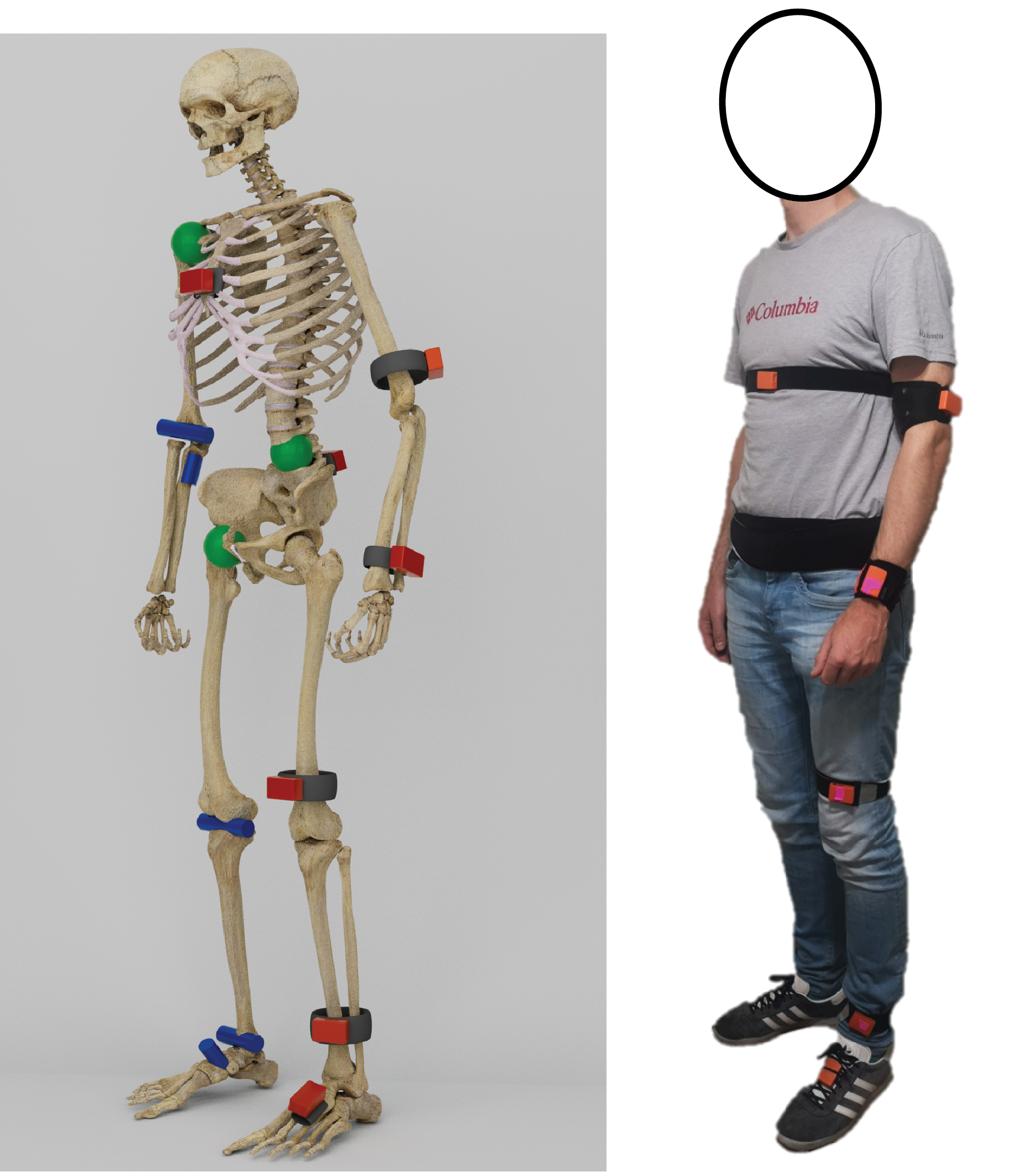
Figure 2. (Left) Our kinematic model with IMUs. Our model includes 10 hinge joints shown in blue and 5 ball-and-socket joints shown in green, resulting in 31 degrees of freedom. IMU location canditates are shown in orange. (Right) User instrumented with IMUs.

We present Diffusion Inertial Poser (DiffIP), a framework capable of reconstructing whole-body human motion in real-time based on sparse IMUs in arbitrary configurations. We first introduce our skeleton model and assumptions on IMU configurations. Then, we explain our diffusion model and how we use it to reconstruct motion. Finally, we discuss the synthesis of our dataset.

3.1. Skeleton model and IMU instrumentation

We used the Lai musculoskeletal model (Lai et al., 2017) from OpenSim. This model comprises 31 degrees of freedom (pelvis [6], hip [3], knee [1], ankle [1], subtalar [1], lumbar [3], shoulder [3], and elbow [2]). The translational and orientation offsets between different joints are physiologically realistic. For example, the knee joint rotation axis translates and rotates as a function of the knee angle.

We assume IMUs to be attached at specific locations for every instrumented body segment (Fig. 2). These attachment points should be respected at inference as they are used to synthesize the training data (Section 3.4). For the upper and lower limbs we opted to attach the sensors in positions as distal as possible without hampering joint motion. As location within a body segment does not influence the orientation estimate of a body, we choose this placement to maximize the signal-to-noise ratio for the measured linear acceleration. The pelvis IMU is attached between the left and right posterior superior iliac spine as this location typically provides an articulation between sensor and body segment with few soft tissue artifacts. The torso IMU is attached at the sternum for the same reason.

3.2. Diffusion Model

3.2.1. Features

Our diffusion model generates sequences of N=61 feature vectors. The feature vector is chosen to represent whole-body pose and IMU information in a compact manner:

(1) $$\bm{x}=(\bm{R},\mathbf{a},\Delta\bm{p},h).$$

$\bm{R}\in\mathbb{R}^{16\times 6}$ are the orientations of the body segments, parameterized by 6-DOF representation of the rotation matrix (Zhou et al., 2019). The orientations for the 12 body segments that are potentially instrumented also represent IMU orientation estimates as there is no relative orientation between IMU and body segment after calibration. $\bm{a}\in\mathbb{R}^{12\times 3}$ are the linear accelerations of the IMU locations on all the potentially instrumented body segments. To complete our whole-body motion representation we have $\Delta\bm{p}$, the 2D change in root position, and $h$ the root height. The full feature matrix is $\bm{x}\in\mathbb{R}^{61\times 135=61\times(16\times 6+12\times 3+2+1)}$.

For the heel and toe of each foot, our model additionally predicts a contact probability $\bm{b}\in\mathbb{R}^{61\times 4}$ that will be used to regularize the generated motion (Section 3.2.3).

3.2.2. Diffusion Framework

Figure 3. DiffIP transformer network. Architecture of the denoiser $\bm{f}_{\theta}(\mathbf{x}_{t},t,c)$ that predicts the sample ($\hat{\bm{x}}_{0}$) and a contact label ($\hat{\bm{b}}_{0}$) given the noised sample $\bm{x}_{t}$, denoising step $t$ and the condition $c$. We use the transformer encoder architecture from (Vaswani et al., 2017) and concatenate a step embedding and condition embedding to the input embedding.

Our diffusion framework is similar to (Tevet et al., 2023; Tseng et al., 2023). Diffusion is modeled as a Markov noising process with latents $\{\bm{x}_{t}\}_{t=0:T}$, where $T=1000$ is the number of diffusion steps. The forward noising process is defined as:

(2) $$q(\bm{x}_{t}|\bm{x})\sim\mathcal{N}(\sqrt{\overline{\alpha}_{t}}\bm{x},(1-\overline{\alpha}_{t})\bm{I})$$

where $\overline{\alpha}_{t}\in[0,1]$ are constants which follow a monotonically decreasing (cosine) schedule for increasing $t$, such that $\bm{x}_{T}\sim\mathcal{N}(0,\bm{I})$. We learn an approximation of the reverse diffusion process, i.e., the denoising process, by training a transformer neural network $\bm{f}_{\theta}$ (Fig. 3), with parameters $\theta$, which takes a noised version $\bm{x}_{t}$ of the ground truth motion $\bm{x}$, the noise step $t$ and condition $c$ and generates a denoised version $\hat{\bm{x}}_{0}$ that aims to match $\bm{x}$:

(3) $$\bm{f}_{\theta}(\bm{x}_{t},t,c)=\hat{\bm{x}}_{0}\approx\bm{x}.$$

We facilitate reconstruction of ground truth motion $\bm{x}$, by providing the height of the subject performing the motion as a condition input $c$ to the network. The intuition to add height as condition is that height is associated with body segment lengths, which mathematically underlie the relation between body orientations and body accelerations and, body orientations and root motion.

3.2.3. Training procedure and losses

For training $\bm{f}_{\theta}$ we follow DDPM (Ho et al., 2020) by sampling a diffusion step from a uniform distribution $U\in[0,T]$, randomly sampling a motion sequence from our training dataset, noising this motion $\bm{x}$ to $\bm{x}_{t}$, predicting $\hat{\bm{x}}_{0}$ and performing gradient descent on our loss $\mathcal{L}$

(4) $$\mathop{\mathbb{E}}_{\bm{x},t}\mathcal{L}(\hat{\bm{x}}_{0},\bm{x}).$$

Similar to (Tseng et al., 2023), our loss is composed of a simple loss (Ho et al., 2020; Tevet et al., 2023) and several auxilary losses:

(5) $$\mathcal{L}=\mathcal{L}_{\rm simple}+\mathcal{L}_{\rm vel}+\mathcal{L}_{\rm FK}+\mathcal{L}_{\rm drift}+\mathcal{L}_{\rm contact}+\mathcal{L}_{\rm slide}$$

with

(6) $$\mathcal{L}_{\rm simple} =\sum_{i=1}^{N}||\hat{\bm{x}}_{0}^{(i)}-\bm{x}^{(i)}||^{2},$$

(7) $$\mathcal{L}_{\rm vel} =\sum_{i=1}^{N-1}||(\hat{\bm{R}}_{0}^{(i+1)}-\hat{\bm{R}}_{0}^{(i)})-(\bm{R}^{(i+1)}-\bm{R}^{(i)})||^{2},$$

(8) $$\mathcal{L}_{\rm FK} =\sum_{i=1}^{N}||{\rm FK}(\hat{\bm{R}}_{0}^{(i)})-{\rm FK}(\bm{R}^{(i)})||^{2},$$

(9) $$\mathcal{L}_{\rm drift} =\sum_{i=1}^{N}||\hat{\bm{p}}_{0}^{(i)}-\bm{p}^{(i)}||^{2}\;\;{\rm where}\;\;\bm{p}^{(i)}=\sum_{j=1}^{i}\Delta\bm{p}^{(j)},$$

(10) $$\mathcal{L}_{\rm contact} =\sum_{i=1}^{N}||\hat{\bm{b}}_{0}^{(i)}-\bm{b}^{(i)}||^{2},$$

(11) $$\mathcal{L}_{\rm slide} =\sum_{i=1}^{N-1}||\hat{\bm{b}}_{0}^{(i)}\cdot[{\rm FK}_{\rm foot}(\hat{\bm{R}}_{0}^{(i+1)})-{\rm FK}_{\rm foot}(\hat{\bm{R}}_{0}^{(i)})+\bm{\Delta p}_{0}^{(i)}]||^{2}.$$

$\mathcal{L}_{\rm vel}$ encourages smooth motion (Petrovich et al., 2021). $\mathcal{L}_{\rm FK}$ is a kinematic loss to encourage realistic joint positions (Shi et al., 2020), with ${\rm FK}$ a function parametrized by the subject-specific skeleton joint offsets that maps body segment orientations to joint locations relative to the root. Compared to prior work we explicitly add $\mathcal{L}_{\rm drift}$, which penalizes drift by accumulating the absolute root translation error across frames. $\mathcal{L}_{\rm drift}$ is required because we choose to predict $\Delta\bm{p}$, rather than $\bm{p}$; a design choice to improve performance when generative motion models are used autoregressively (Rempe et al., 2021). $\mathcal{L}_{\rm contact}$ is an auxilary loss to predict a reliable contact probability $\hat{\bm{b}}$ that is fed to $\mathcal{L}_{\rm slide}$. $\mathcal{L}_{\rm slide}$ encourages the model to generate motion where foot motion is consistent with foot contact prediction (i.e., minimizing foot velocity when in contact) (Tseng et al., 2023).

3.3. Inference

During inference we run a denoising process to go from a standard Gaussian noise sample, $\bm{x}_{T}$, to a final denoised prediction, $\hat{\bm{x}}_{0,{\rm final}}$ (Algorithm 1). Editing can be leveraged to enforce consistency with a partially known motion, $\bm{x}^{\rm known}$, or to enforce temporal consistency between multiple generated sequences. To edit a motion sequence, we rely on a mask $\bm{m}^{61\times 135}$ that indicates which features and frames from $\bm{x}^{\rm known}$ need to be respected in the predicted motion.

Given : $c,\bm{m},\bm{x}^{\rm known}$

$\bm{x}_{T}\sim\mathcal{N}(\bm{0},\bm{I})$

for t=999…2 do

       predict $\hat{\bm{x}}_{0}=p_{\theta}(\bm{x}_{t},t,c)$

       if editing then

             $\hat{\bm{x}}_{0}=\bm{m}\odot\bm{x}^{\rm known}+(1-\bm{m})\odot\hat{\bm{x}}_{0}$

       noise $\bm{x}_{t-1}\sim\mathcal{N}(\sqrt{\overline{\alpha}_{t}}\bm{\hat{\bm{x}}_{0}},(1-\overline{\alpha}_{t})\bm{I})$

end for

predict $\hat{\bm{x}}_{0,\rm final}=p_{\theta}(\bm{x}_{1},1,c)$

ALGORITHM 1 Inferencing DiffIP

During online motion reconstruction we stream IMU measurements at 20Hz. Every 50ms we get access to a new partially known $\bm{x}^{(N)}$ and can rely on our previous prediction and acquired IMU measurements for $\bm{x}^{(1:N-1)}$. We concatenate these along the time dimension to form $\bm{x}^{\rm known}$ and apply the editing procedure to predict the unmeasured part of $\bm{x}^{(N)}$ using a mask: $\bm{m}=[\bm{1}^{(N-1)\times 135};\bm{m}_{\rm IMU}]$, with $\bm{m}_{\rm IMU}$ a vector of 0s and 1s, with 1s for the features that correspond to the IMU measurements. Every frame thus requires a denoising process. To enable this at 20Hz we reduce the number of denoising steps to five. It has been shown that generative diffusion models can be deployed more efficiently by performing fewer denoising steps without significant loss in performance (Du et al., 2023). We confirm that such reduction is applicable to our case (Section 4.3).

3.4. Data

Since no large dataset of motion synthesized with OpenSim models exists, we created one from existing marker-based optical motion capture datasets. We synthesized motions and associated musculoskeletal models scaled to subject anthropometry. To this end, we used AddBiomechanics, a new tool that automates the estimation of joint kinematics from marker data (Werling et al., 2022). We used marker-based optical motion capture data from three existing datasets (Joo et al., 2015; Szczesna et al., 2021; Trumble et al., 2017) to synthesize motions. The aggregated dataset comprises data from 339 subjects and 3350 trials. We synthesized IMU signals for each trial in our dataset given the scaled skeleton model and the generalized coordinates. IMU orientations were generated as the global orientations of the bodies. IMU linear accelerations were derived by double differentation of the IMU positions that were obtained by a forward kinematic pass. Linear accelerations are averaged at the original sampling rate using a moving average sliding window of 166ms (e.g., 11 frames at 60Hz) (Jiang et al., 2022). Finally, all timeseries are resampled at 20Hz. Ground-truth contact labels were annotated by applying a velocity threshold (0.3m/s) for each of the four potential contact points (heels and toes).

4. Evaluations

We run several experiments and evaluations to quantify reconstruction performance for different IMU configurations, analyze sim-to-real transfer and compare DiffIP to TIP (Jiang et al., 2022). Next, we show that DiffIP, which is a generative model, performs better than a regressive model that allows motion reconstruction from arbitrary configurations as well. Finally, we have a live demonstration.

4.0.1. Evaluation Datasets

We use the TotalCapture dataset with real IMU data (Trumble et al., 2017) to evaluate sim-to-real transfer and compare DiffIP to TIP. We omitted 3 of 43 trials in TotalCapture because marker data was poorly labeled. Next, we use one hour of motion data across 334 trials as a test split from our original synthetic dataset to evaluate performance. We choose this test split rather than TotalCapture to evaluate our DiffIP beyond sim-to-real transfer as it contains a wider variety of motions. In contrast to prior works, we do not use DIP-IMU, or DanceDB as no marker data is available for these datasets and we therefore cannot reconstruct ground truth for our OpenSim skeleton.

4.0.2. Metrics

We adopt the same evaluation metrics as TIP:

• Mean Joint Orientation Error, MJOE [^∘]: Magnitude of the axis-angle representation of the rotation difference between ground-truth and reconstructed joint angle.

• Mean Joint Position Error, MJPE [$cm$]: Difference (Euclidean norm) of the joint Cartesian position relative to the root between ground-truth and reconstructed joint positions.

• Root Translation Error, RTE [$m$]: Difference (Euclidean norm) of the root position between ground-truth and reconstructed motion at 2s and 10s into the motion.

All metrics are averaged over time, trials and joints. We omit reporting root and joint position jitter. Although this is a common measure in prior work (Jiang et al., 2022; Yi et al., 2022, 2021), we find this measure not very representative. Calculating jerk by finite differencing a signal at 20Hz is spurious and our ground truth motion, that we synthesized using AddBiomechanics (Section 3.4), has higher jitter values than predicted motion in prior work.

Unless specified otherwise, metrics result from comparing ground truth and predicted motion using five denoising steps. We focus on results for the cases of instrumenting the body with six, four or three IMUs. We report and discuss results for the configurations depicted in Table 1 as these predict motions with the lowest errors for either the pose or the root translation. More extensive testing across configurations is presented in the Appendix.

Table 1. Selected configurations for which we tested DiffIP.

$\rm pelvis$

$\rm thigh_{R}$

$\rm shank_{R}$

$\rm foot_{R}$

$\rm thigh_{L}$

$\rm shank_{L}$

$\rm foot_{L}$

$\rm torso$

$\rm upperarm_{R}$

$\rm forearm_{R}$

$\rm upperarm_{L}$

$\rm forearm_{L}$

DiffIP-6A

X

X

X

X

X

X

DiffIP-6C

X

X

X

X

X

X

DiffIP-4A

X

X

X

X

DiffIP-4C

X

X

X

X

DiffIP-3A

X

X

X

DiffIP-3D

X

X

X

4.1. Optimal configuration given a number of IMUs

From evaluations on the test split we find the optimal IMU configuration given a specific number of IMUs (Table 1 and Table 2). In the case of using six IMUs, it is best to have one on the torso and one on the pelvis. For the remaining four IMUs or when only using four IMUs, it is best to attach two to the forearms and two to the lower limbs. Attaching the lower limb IMUs to the feet leads to lower root translation errors but gives slightly worse joint pose estimation compared to attaching them to the thighs. Foot acceleration gives useful information concerning contact, explaining why their presence reduces foot sliding and root translation error. This finding is consistent throughout experiments and during live demonstration.

The increase in joint orientation and position errors when attaching the IMUs to the feet rather than the thighs is small and only obvious in specific motions. Our video shows an example of a subject sitting down where DiffIP-6C outperforms DiffIP-6A: the thigh IMUs guide the prediction to remain in a seated position whereas the feet IMUs do not provide this guidance.

When instrumenting with three sensors it is optimal to attach them asymmetrically and cover the kinematic chain: right foot, pelvis and left forearm or left foot, pelvis, and right forearm.

As expected, all error metrics increase when using fewer IMUs. When using three sensors our MJOE metric is lower than the one reported in (Mollyn et al., 2023), the only other system we are aware of that is reconstructing motion from three IMUs. However, it is hard to compare the two systems as different test sets are used and their sensors might be less accurate as they use IMUs embedded in phones, earbuds and watches.

Table 2. Evaluation of motion reconstruction performance across selected IMU configurations.

Test split
	MJOE [∘]	MJPE [cm]	RTE2s [m]	RTE10s [m]
DiffIP-6A	14.7	7.5	$\mathbf{0.15}$	$\mathbf{0.36}$
DiffIP-6C	$\mathbf{13.6}$	$\mathbf{7.1}$	0.16	0.57
DiffIP-4A	16.0	9.2	$\mathbf{0.17}$	$\mathbf{0.45}$
DiffIP-4C	$\mathbf{16.0}$	$\mathbf{8.8}$	0.20	0.70
DiffIP-3A	22.2	13.3	$\mathbf{0.17}$	$\mathbf{0.53}$
DiffIP-3D	$\mathbf{19.2}$	$\mathbf{11.6}$	0.20	0.79

4.2. Sim-to-real transfer and comparison to TIP

We compare performance for our six IMU sensor configurations to TIP (Jiang et al., 2022) in Table 3. TIP is, concurrent with PIP, the state-of-the-art for the six IMU configuration. Due to the differences in the OpenSim skeleton and SMPL skeleton used in (Jiang et al., 2022), we need to establish joint correspondence when calculating MJOE and MJPE. For each joint in OpenSim, we found the closest corresponding joint in SMPL. Joints on the limbs can be exactly mapped between skeletons, but SMPL has many more joints proximal to the root which are not all included in the metric calculation. Although the mapping for these proximal joints is not exact between skeletons, we found that proximal joints nevertheless have low position error compared to joints on the limbs, as the error increases when progressing along the kinematic tree. We ran evaluations on the full-length of trials (rather than a randomly selected 10s window for each trial, as done in prior work).

In terms of MJOE and MJPE we found DiffIP is on par with TIP. The root translation error for DiffIP is higher. Where TIP reduces root drift by exploiting the stable-boundary-points predictions, we do not perform any correction and leave this for future work to be incorporated. Error metrics on the TotalCapture real IMU dataset are lower than on the test split in most configurations. This results from the test split containing more motion variation.

Table 3. Evaluation on TotalCapture with real IMU data and comparison to TIP. Boldfaced are the lowest errors in a comparison between TIP and DiffIP.

TotalCapture real IMU
	MJOE [∘]	MJPE [cm]	RTE2s [m]	RTE10s [m]
TIP	$\bm{12.1}$	6.8	0.13	$\bm{0.23}$
DiffIP-6A	13.6	6.3	$\bm{0.08}$	0.35
DiffIP-6C	13.4	$\bm{6.2}$	0.09	0.55
DiffIP-4A	14.7	7.8	0.08	0.37
DiffIP-4C	14.6	7.6	0.09	0.81
DiffIP-3A	19.7	11.9	0.09	0.50
DiffIP-3D	18.6	10.8	0.09	0.82

4.3. Effect of reducing the number of denoising steps

For DiffIP to run online we reduce the denoising process to the last five denoising steps. Similar to (Du et al., 2023), we ablate the number of sampling steps that we use during inference to understand the effect on motion reconstruction (Table 4). We test DiffIP with a subset of denoising steps during inference on the test split data. We find that beyond five denoising steps, predictions do not improve on our chosen metrics. High quality predictions of DiffIP with a only five denoising steps is possible due to the strong guidance that is provided by editing during inference, as we edit based on all but the last frame and for that last frame we have partially known features (i.e., measurements).

Table 4. Evaluation of decreasing numbers of denoising steps.

Test split
	#steps	MJOE [∘]	MJPE [cm]	RTE2s [m]	RTE10s [m]
DiffIP-6A	1000	14.7	7.5	0.15	0.36
DiffIP-6A	100	14.7	7.5	0.15	0.36
DiffIP-6A	10	14.6	7.5	0.15	0.34
DiffIP-6A	5	14.7	7.5	0.15	0.36
DiffIP-6A	1	22.8	16.1	0.29	1.0

4.4. Diffusion model vs regressive model

We compare performance of DiffIP, which is a generative model against a regression model using a conditional transformer (c-trans). We chose the same transformer architecture for c-trans as for DiffIP and concatenate a mask that represents the IMU configuration to the input features. During training we randomly sample across IMU configurations and mask out the non-measured parts of the feature vector for the final frame. The first 60 frames are assumed given as input during training, where we dropout 80% of the non-measured features to avoid overfitting (Jiang et al., 2022; Srivastava et al., 2014). As we will deploy this transformer in an online autoregressive fashion we only care about predicting the last frame. At inference, we shift the latest prediction into the history at every new frame.

DiffIP performs better than c-trans across different IMU configurations (Table 5). From analyzing c-trans predictions we found that for some trials it is on par with DiffIP while it fails in other cases. We attribute robustness of DiffIP to its generative nature.

Table 5. Evaluation of a conditional transformer fulfilling the task of DiffIP.

TotalCapture real IMU
	MJOE [∘]	MJPE [cm]	RTE2s [m]	RTE10s [m]
c-trans-6A	19.1	11.8	0.24	1.15
c-trans-4A	22.5	14.7	0.27	1.47
c-trans-3A	25.9	18.1	0.32	1.58

4.5. Live demonstration

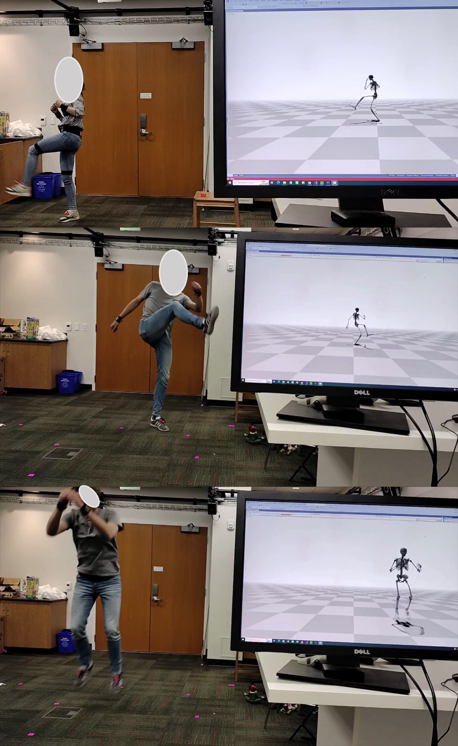
Figure 4. DiffIP used by different subjects wearing XSens IMUs. There is about 150ms delay between real motion and visualization. Upper. Configuration IMU-3A: the reconstruction of the legs is good while arm motion is inpainted by the diffusion model. Middle. Configuration IMU-4A: performing a soccer kick. Lower. Configuration IMU-4A: performing a jump.

We test our system live with different IMU configurations: DiffIP-6A, DiffIP-4A and DiffIP-3A. We use XSens IMU sensors and stream processed (MTw Awinda) orientation and linear acceleration at 60Hz. We apply a moving average filter with current frame and five past and five future frames on the acceleration and downsample both signals to 20Hz to match our synthetic training data. We cover a variety of motions including walking, jogging, jumping, squatting and kicking (Fig. 4). Our live demo results can be observed in the supplementary video. Reconstruction quality degrades when using fewer IMUs, but uninstrumented limbs are predicted to do realistic motion as is expected with the use of a generative model. In the videos there is latency between the real and visualized motion. We ran our algorithm with five denoising steps, which takes about 25ms to evaluate. The total latency is the result from (1) XSens to system communication and run-time of our own algorithm (2) moving average filter (83ms) and (3) our algorithm ($\sim$25ms). The latency of the motion reconstruction algorithm is slightly more than TIP (90ms) (Jiang et al., 2022), and significantly more than PIP (16ms) (Yi et al., 2022).

5. Conclusion

This paper presents DiffIP, a single pretrained generative model that can reconstruct whole-body human motion from arbitrary IMU configurations in real-time. The use of a generative model provides robustness in motion prediction against sparsity and noisy sensor measurements. Our evaluations show state-of-the-art performance for previously used IMU configuration including six sensors and little degradation in performance when using less sensors. DiffIP has applications in health and human performance where users can select a configuration that suits their goal best.

Future work could address some of the current limitations of DiffIP. The latency of DiffIP ($\sim$110ms) can form a limitation for applications that require shorter latencies such as visual illusion (¡50ms according to (Stauffert et al., 2020)) or control of an assistive device (e.g., 40-60ms to assist balance with an exoskeleton according to (Beck et al., 2023)). Root drift and foot sliding could be improved by incorporating physics (Yi et al., 2022) or heuristics (Jiang et al., 2022). Extending the dataset for OpenSim models could help with reconstructing more extreme motions that were currently not predicted accurately by DiffIP (e.g., lunges and cart wheel). Finally, an extension of the system that allows estimation of joint torques (Yuan et al., 2022) and muscle forces could lead to a breakthrough system for biomechanists and users interested in health and performance.

References

- (1)
- Ahuja and Morency (2019) Chaitanya Ahuja and Louis-Philippe Morency. 2019. Language2Pose: Natural Language Grounded Pose Forecasting. 2019 International Conference on 3D Vision (3DV) (2019), 719–728.
- Arnold et al. (2006) Allison S. Arnold, May Q. Liu, Michael H. Schwartz, Sylvia Õunpuu, and Scott L. Delp. 2006. The role of estimating muscle-tendon lengths and velocities of the hamstrings in the evaluation and treatment of crouch gait. Gait and Posture 23, 3 (2006), 273–281. https://doi.org/10.1016/j.gaitpost.2005.03.003
- Beck et al. (2023) Owen N Beck, Max K Shepherd, Rish Rastogi, Giovanni Martino, Lena H Ting, and Gregory S Sawicki. 2023. Exoskeletons need to react faster than physiological responses to improve standing balance. Science robotics 8, 75 (2023), eadf1080.
- Dembia et al. (2021) Christopher L. Dembia, Nicholas A. Bianco, Antoine Falisse, Jennifer L. Hicks, and Scott L. Delp. 2021. OpenSim Moco: Musculoskeletal optimal control. PLOS Computational Biology 16, 12 (12 2021), 1–21. https://doi.org/10.1371/journal.pcbi.1008493
- Du et al. (2023) Yuming Du, Robin Kips, Albert Pumarola, Sebastian Starke, Ali Thabet, and Artsiom Sanakoyeu. 2023. Avatars Grow Legs: Generating Smooth Human Motion from Sparse Tracking Inputs with Diffusion Model. In CVPR.
- Ho et al. (2020) Jonathan Ho, Ajay Jain, and Pieter Abbeel. 2020. Denoising Diffusion Probabilistic Models. arXiv preprint arxiv:2006.11239 (2020).
- Huang et al. (2018) Yinghao Huang, Manuel Kaufmann, Emre Aksan, Michael J. Black, Otmar Hilliges, and Gerard Pons-Moll. 2018. Deep Inertial Poser: Learning to Reconstruct Human Pose from Sparse Inertial Measurements in Real Time. ACM Transactions on Graphics, (Proc. SIGGRAPH Asia) 37 (Nov. 2018), 185:1–185:15. https://doi.org/10.1145/3272127.3275108 Two first authors contributed equally.
- Jiang et al. (2022) Yifeng Jiang, Yuting Ye, Deepak Gopinath, Jungdam Won, Alexander W. Winkler, and C. Karen Liu. 2022. Transformer Inertial Poser: Real-Time Human Motion Reconstruction from Sparse IMUs with Simultaneous Terrain Generation. In SIGGRAPH Asia 2022 Conference Papers (Daegu, Republic of Korea) (SA ’22). Association for Computing Machinery, New York, NY, USA, Article 3, 9 pages. https://doi.org/10.1145/3550469.3555428
- Joo et al. (2015) Hanbyul Joo, Hao Liu, Lei Tan, Lin Gui, Bart Nabbe, Iain Matthews, Takeo Kanade, Shohei Nobuhara, and Yaser Sheikh. 2015. Panoptic Studio: A Massively Multiview System for Social Motion Capture. In The IEEE International Conference on Computer Vision (ICCV).
- Kim et al. (2022) Jihoon Kim, Jiseob Kim, and Sungjoon Choi. 2022. Flame: Free-form language-based motion synthesis and editing. arXiv preprint arXiv:2209.00349 (2022).
- Kingma and Welling (2013) Diederik P Kingma and Max Welling. 2013. Auto-encoding variational bayes. arXiv preprint arXiv:1312.6114 (2013).
- Lai et al. (2017) Adrian KM Lai, Allison S Arnold, and James M Wakeling. 2017. Why are antagonist muscles co-activated in my simulation? A musculoskeletal model for analysing human locomotor tasks. Annals of biomedical engineering 45 (2017), 2762–2774.
- Lee and Lee (2022) Chang June Lee and Jung Keun Lee. 2022. Inertial motion capture-based wearable systems for estimation of joint kinetics: A systematic review. Sensors 22, 7 (2022), 2507.
- Li et al. (2023) Jiaman Li, C. Karen Liu, and Jiajun Wu. 2023. Ego-Body Pose Estimation via Ego-Head Pose Estimation. arXiv:2212.04636 [cs.CV]
- Loper et al. (2015) Matthew Loper, Naureen Mahmood, Javier Romero, Gerard Pons-Moll, and Michael J. Black. 2015. SMPL: A Skinned Multi-Person Linear Model. ACM Trans. Graph. 34, 6, Article 248 (nov 2015), 16 pages. https://doi.org/10.1145/2816795.2818013
- Mahmood et al. (2019) Naureen Mahmood, Nima Ghorbani, Nikolaus F. Troje, Gerard Pons-Moll, and Michael J. Black. 2019. AMASS: Archive of Motion Capture as Surface Shapes. In International Conference on Computer Vision. 5442–5451.
- Malleson et al. (2017) Charles Malleson, Andrew Gilbert, Matthew Trumble, John Collomosse, Adrian Hilton, and Marco Volino. 2017. Real-Time Full-Body Motion Capture from Video and IMUs. In 2017 International Conference on 3D Vision (3DV). 449–457. https://doi.org/10.1109/3DV.2017.00058
- Mollyn et al. (2023) Vimal Mollyn, Riku Arakawa, Mayank Goel, Chris Harrison, and Karan Ahuja. 2023. IMUPoser: Full-Body Pose Estimation Using IMUs in Phones, Watches, and Earbuds. In Proceedings of the 2023 CHI Conference on Human Factors in Computing Systems (Hamburg, Germany) (CHI ’23). Association for Computing Machinery, New York, NY, USA, Article 529, 12 pages. https://doi.org/10.1145/3544548.3581392
- Petrovich et al. (2021) Mathis Petrovich, Michael J. Black, and Gül Varol. 2021. Action-Conditioned 3D Human Motion Synthesis with Transformer VAE. In International Conference on Computer Vision (ICCV).
- Petrovich et al. (2022) Mathis Petrovich, Michael J. Black, and Gül Varol. 2022. TEMOS: Generating diverse human motions from textual descriptions. In European Conference on Computer Vision (ECCV).
- Rempe et al. (2021) Davis Rempe, Tolga Birdal, Aaron Hertzmann, Jimei Yang, Srinath Sridhar, and Leonidas J. Guibas. 2021. HuMoR: 3D Human Motion Model for Robust Pose Estimation. In International Conference on Computer Vision (ICCV).
- Ren et al. (2023) Yiming Ren, Chengfeng Zhao, Yannan He, Peishan Cong, Han Liang, Jingyi Yu, Lan Xu, and Yuexin Ma. 2023. LiDAR-aid Inertial Poser: Large-scale Human Motion Capture by Sparse Inertial and LiDAR Sensors. IEEE Transactions on Visualization and Computer Graphics 29, 5 (2023), 2337–2347. https://doi.org/10.1109/TVCG.2023.3247088
- Roetenberg et al. (2009) Daniel Roetenberg, Henk Luinge, Per Slycke, et al. 2009. Xsens MVN: Full 6DOF human motion tracking using miniature inertial sensors. Xsens Motion Technologies BV, Tech. Rep 1 (2009), 1–7.
- Schepers et al. (2018) Martin Schepers, Matteo Giuberti, Giovanni Bellusci, et al. 2018. Xsens MVN: Consistent tracking of human motion using inertial sensing. Xsens Technol 1, 8 (2018).
- Schreiner et al. (2021) Paul Schreiner, Maksym Perepichka, Hayden Lewis, Sune Darkner, Paul G. Kry, Kenny Erleben, and Victor B. Zordan. 2021. Global Position Prediction for Interactive Motion Capture. Proc. ACM Comput. Graph. Interact. Tech. 4, 3, Article 39 (sep 2021), 16 pages. https://doi.org/10.1145/3479985
- Seth et al. (2018) Ajay Seth, Jennifer L Hicks, Thomas K Uchida, Ayman Habib, Christopher L Dembia, James J Dunne, Carmichael F Ong, Matthew S DeMers, Apoorva Rajagopal, Matthew Millard, et al. 2018. OpenSim: Simulating musculoskeletal dynamics and neuromuscular control to study human and animal movement. PLoS computational biology 14, 7 (2018), e1006223.
- Shi et al. (2020) Mingyi Shi, Kfir Aberman, Andreas Aristidou, Taku Komura, Dani Lischinski, Daniel Cohen-Or, and Baoquan Chen. 2020. MotioNet: 3D Human Motion Reconstruction from Monocular Video with Skeleton Consistency. ACM Trans. Graph. 40, 1, Article 1 (sep 2020), 15 pages. https://doi.org/10.1145/3407659
- Slyper and Hodgins (2008) Ronit Slyper and Jessica K. Hodgins. 2008. Action Capture with Accelerometers (SCA ’08). Eurographics Association, Goslar, DEU, 193–199.
- Sohl-Dickstein et al. (2015) Jascha Sohl-Dickstein, Eric Weiss, Niru Maheswaranathan, and Surya Ganguli. 2015. Deep Unsupervised Learning using Nonequilibrium Thermodynamics. In Proceedings of the 32nd International Conference on Machine Learning (Proceedings of Machine Learning Research, Vol. 37), Francis Bach and David Blei (Eds.). PMLR, Lille, France, 2256–2265. https://proceedings.mlr.press/v37/sohl-dickstein15.html
- Srivastava et al. (2014) Nitish Srivastava, Geoffrey Hinton, Alex Krizhevsky, Ilya Sutskever, and Ruslan Salakhutdinov. 2014. Dropout: a simple way to prevent neural networks from overfitting. The journal of machine learning research 15, 1 (2014), 1929–1958.
- Stauffert et al. (2020) Jan-Philipp Stauffert, Florian Niebling, and Marc Erich Latoschik. 2020. Latency and cybersickness: Impact, causes, and measures. A review. Frontiers in Virtual Reality 1 (2020), 582204.
- Szcz\kesna et al. (2021) Agnieszka Szcz\kesna, Monika Błaszczyszyn, and Magdalena Pawlyta. 2021. Optical motion capture dataset of selected techniques in beginner and advanced Kyokushin karate athletes. Scientific Data 8, 1 (2021), 13.
- Tautges et al. (2011) Jochen Tautges, Arno Zinke, Björn Krüger, Jan Baumann, Andreas Weber, Thomas Helten, Meinard Müller, Hans-Peter Seidel, and Bernd Eberhardt. 2011. Motion Reconstruction Using Sparse Accelerometer Data. 30, 3, Article 18 (may 2011), 12 pages. https://doi.org/10.1145/1966394.1966397
- Tevet et al. (2023) Guy Tevet, Sigal Raab, Brian Gordon, Yoni Shafir, Daniel Cohen-or, and Amit Haim Bermano. 2023. Human Motion Diffusion Model. In The Eleventh International Conference on Learning Representations. https://openreview.net/forum?id=SJ1kSyO2jwu
- Trumble et al. (2017) Matt Trumble, Andrew Gilbert, Charles Malleson, Adrian Hilton, and John Collomosse. 2017. Total Capture: 3D Human Pose Estimation Fusing Video and Inertial Sensors. In 2017 British Machine Vision Conference (BMVC).
- Tseng et al. (2023) Jonathan Tseng, Rodrigo Castellon, and C. Karen Liu. 2023. EDGE: Editable Dance Generation From Music. arXiv:2211.10658 [cs.SD]
- Uhlrich et al. (2022) Scott D Uhlrich, Antoine Falisse, Łukasz Kidziński, Julie Muccini, Michael Ko, Akshay S Chaudhari, Jennifer L Hicks, and Scott L Delp. 2022. OpenCap: 3D human movement dynamics from smartphone videos. bioRxiv (2022), 2022–07.
- Uhlrich et al. (2023) Scott D. Uhlrich, Thomas K. Uchida, Marissa R. Lee, and Scott L. Delp. 2023. Ten steps to becoming a musculoskeletal simulation expert: A half-century of progress and outlook for the future. Journal of Biomechanics 154 (2023), 111623. https://doi.org/10.1016/j.jbiomech.2023.111623
- Vaswani et al. (2017) Ashish Vaswani, Noam Shazeer, Niki Parmar, Jakob Uszkoreit, Llion Jones, Aidan N. Gomez, Łukasz Kaiser, and Illia Polosukhin. 2017. Attention is All You Need. In Proceedings of the 31st International Conference on Neural Information Processing Systems (Long Beach, California, USA) (NIPS’17). Curran Associates Inc., Red Hook, NY, USA, 6000–6010.
- Von Marcard et al. (2017) Timo Von Marcard, Bodo Rosenhahn, Michael J Black, and Gerard Pons-Moll. 2017. Sparse inertial poser: Automatic 3d human pose estimation from sparse imus. In Computer graphics forum, Vol. 36. Wiley Online Library, 349–360.
- Werling et al. (2022) Keenon Werling, Michael Raitor, Jon Stingel, Jennifer L Hicks, Steve Collins, Scott Delp, and C Karen Liu. 2022. Rapid bilevel optimization to concurrently solve musculoskeletal scaling, marker registration, and inverse kinematic problems for human motion reconstruction. bioRxiv (2022), 2022–08.
- Wouda et al. (2018) Frank J. Wouda, Matteo Giuberti, Giovanni Bellusci, Erik Maartens, Jasper Reenalda, Bert-Jan F. Van Beijnum, and Peter H. Veltink. 2018. On the Validity of Different Motion Capture Technologies for the Analysis of Running. In 2018 7th IEEE International Conference on Biomedical Robotics and Biomechatronics (Biorob). 1175–1180. https://doi.org/10.1109/BIOROB.2018.8487210
- Yi et al. (2022) Xinyu Yi, Yuxiao Zhou, Marc Habermann, Soshi Shimada, Vladislav Golyanik, Christian Theobalt, and Feng Xu. 2022. Physical Inertial Poser (PIP): Physics-aware Real-time Human Motion Tracking from Sparse Inertial Sensors. In IEEE/CVF Conference on Computer Vision and Pattern Recognition (CVPR).
- Yi et al. (2021) Xinyu Yi, Yuxiao Zhou, and Feng Xu. 2021. TransPose: Real-Time 3D Human Translation and Pose Estimation with Six Inertial Sensors. ACM Trans. Graph. 40, 4, Article 86 (jul 2021), 13 pages. https://doi.org/10.1145/3450626.3459786
- Yuan et al. (2022) Ye Yuan, Jiaming Song, Umar Iqbal, Arash Vahdat, and Jan Kautz. 2022. PhysDiff: Physics-Guided Human Motion Diffusion Model. arXiv preprint arXiv:2212.02500 (2022).
- Zhang et al. (2022) Mingyuan Zhang, Zhongang Cai, Liang Pan, Fangzhou Hong, Xinying Guo, Lei Yang, and Ziwei Liu. 2022. MotionDiffuse: Text-Driven Human Motion Generation with Diffusion Model. arXiv preprint arXiv:2208.15001 (2022).
- Zheng et al. (2018) Zerong Zheng, Tao Yu, Hao Li, Kaiwen Guo, Qionghai Dai, Lu Fang, and Yebin Liu. 2018. HybridFusion: Real-Time Performance Capture Using a Single Depth Sensor and Sparse IMUs. In Proceedings of the European Conference on Computer Vision (ECCV).
- Zhou et al. (2019) Yi Zhou, Connelly Barnes, Jingwan Lu, Jimei Yang, and Hao Li. 2019. On the Continuity of Rotation Representations in Neural Networks. In 2019 IEEE/CVF Conference on Computer Vision and Pattern Recognition (CVPR). 5738–5746. https://doi.org/10.1109/CVPR.2019.00589