Communication-Efficient Decentralized Federated Learning via One-Bit Compressive Sensing

Abstract

Decentralized federated learning (DFL) has gained popularity due to its practicality across various applications. Compared to the centralized version, training a shared model among a large number of nodes in DFL is more challenging, as there is no central server to coordinate the training process. Especially when distributed nodes suffer from limitations in communication or computational resources, DFL will experience extremely inefficient and unstable training. Motivated by these challenges, in this paper, we develop a novel algorithm based on the framework of the inexact alternating direction method (iADM). On one hand, our goal is to train a shared model with a sparsity constraint. This constraint enables us to leverage one-bit compressive sensing (1BCS), allowing transmission of one-bit information among neighbour nodes. On the other hand, communication between neighbour nodes occurs only at certain steps, reducing the number of communication rounds. Therefore, the algorithm exhibits notable communication efficiency. Additionally, as each node selects only a subset of neighbours to participate in the training, the algorithm is robust against stragglers. Additionally, complex items are computed only once for several consecutive steps and subproblems are solved inexactly using closed-form solutions, resulting in high computational efficiency. Finally, numerical experiments showcase the algorithm’s effectiveness in both communication and computation.

I Introduction

Federated learning (FL [1, 2]), a recent cutting-edge technology in machine learning, has found diverse applications such as vehicular communications [3, 4, 5, 6], digital health [7], and mobile edge computing [8, 9]. Despite its promising potential, FL still faces many challenges [10, 11, 12], including communication and computation inefficiency, the impact of stragglers, and privacy. In contrast to the popular centralized FL where a central server is involved to coordinate the training across all nodes, DFL aims to train a shared model by achieving consensus among neighbour nodes. Specifically, given $m$ nodes ${{\mathcal{V}}:=\{1,2,\cdots,m\}}$, each node $i{\in{\mathcal{V}}}$ has a loss function ${f_{i}(\cdot):=f_{i}(\cdot;{\mathcal{D}}_{i})}$ associated with private data ${\mathcal{D}}_{i}$, where ${f_{i}:{\mathbb{R}}^{n}{\to}{\mathbb{R}}}$ is continuous and bounded from below. Moreover, each node $i$ can only exchange messages with its neighbour nodes ${j\in{\mathcal{M}}_{i}}$, where ${{\mathcal{M}}_{i}}$ is a subset of ${\mathcal{V}}$ consisting of nodes that connect with node $i$. Overall, we have an undirected graph ${{\mathcal{G}}:=({\mathcal{V}},{\mathcal{E}})}$, where ${{\mathcal{V}}}$ is the set of vertexes and ${{\mathcal{E}}:=\{(i,j):j\in{\mathcal{M}}_{i},i\in{\mathcal{V}}\}}$ is the set of edges. The task is to train a shared parameter $\mathbf{w}^{*}$ by solving the following optimization problem,

$$\begin{array}[]{l}\min_{\mathbf{w}}~{}f(\mathbf{w}):=\sum_{i\in{\mathcal{V}}}f_{i}(\mathbf{w}),~{}~{}{\rm s.t.}~{}\mathbf{w}\in\Omega,\end{array}$$ (2)

where $\Omega$ is a sparsity constraint defined by

$$\Omega:=\{\mathbf{w}\in{\mathbb{R}}^{n}:\|\mathbf{w}\|_{0}\leq s\}.$$

Here, $\|\mathbf{w}\|_{0}$ is the zero norm of $\mathbf{w}$ counting its number of non-zero entries and $s\ll n$ is a given sparsity level. The purpose of incorporating a sparsity constraint in problem (2) is to leverage the technique of 1BCS, which is capable of reducing the communication cost significantly. More details are provided in Section II-A. In the setting of DFL, problem (2) can be rewritten as

$$\begin{array}[]{rll}\min_{{\mathbf{W}}}&{}&\sum_{i\in{\mathcal{V}}}f_{i}(\mathbf{w}_{i}),\\ {\rm s.t.}&&\mathbf{w}_{i}\in\Omega,~{}i\in{\mathcal{V}},~{}~{}\mathbf{w}_{i}=\mathbf{w}_{j},~{}(i,j)\in{\mathcal{E}},\end{array}$$ (5)

where ${{\mathbf{W}}:=(\mathbf{w}_{1},\mathbf{w}_{2},\cdots,\mathbf{w}_{m})\in{\mathbb{R}}^{n\times m}}$. We point out that if graph ${\mathcal{G}}$ is connected, then ${\mathbf{w}_{1}=\mathbf{w}_{2}=\cdots=\mathbf{w}_{m}}$ and thus problems (2) and (5) are equivalent to each other. Therefore, hereafter we always assume the connection of graph ${\mathcal{G}}$.

I-A Prior arts

There is an impressive body of work in designing algorithmic frameworks to address DFL. For instance, a decentralized parallel stochastic gradient descent (D-PSGD) was introduced and studied in [13]. In this approach, each node updates its parameters based on the average of parameters of its neighbours using the SGD scheme. Subsequently, various compressed versions of D-PSGD have been proposed [14, 15, 16]. The fundamental idea behind these algorithms is to compress the exchanged parameters to lessen the transmitted content. Moreover, in the algorithm proposed by [17], local nodes adopted a Bayesian-like approach through the introduction of a belief over the model parameter space. The DFL based on the interplanetary file system [18] relaxed synchronization after each round. In [19], a robust decentralized SGD approach tackled the challenge of unreliable communications by updating model parameters with partially received messages and optimizing mixing weights. Recently, GossipFL [20] enforced nodes to communicate with only one of their neighbour nodes by exchanging sparsified parameters, enhancing communication efficiency significantly. Additional algorithms can be found in [21, 22, 23, 24, 25, 26].

We emphasize that various aforementioned algorithms, such as those discussed in [14, 15, 16, 20], benefit from the techniques of compression to improve the communication efficiency. They compress an original message using a compression operator and then share the compressed message with the others. Consequently, it is common to impose assumptions on the compression operator to restrict the gap between the compressed and original messages [14, 15, 16]. In contrast, this paper aims to compress the original message but transmit the sign of the compressed message. Upon receiving the transmitted one-bit signal, a node exploits the 1BCS technique to recover the original message. Despite incurring some additional computational cost, this approach exhibits the potential to reduce the communication cost, preserve training accuracy, and relax assumptions on the compression operator.

I-B Our contribution

The main contribution of this paper lies in the development of a novel DFL algorithm, which is built upon the iADM and possesses the following advantageous properties.

• Communication efficiency. Due to the integration of a sparsity constraint in the learning model, we harness the 1BCS technique to exchange one-bit signals when two neighbour nodes communicate with each other. Consequently, the transmitted content is significantly lessened. To the best of our knowledge, we have not come across similar efforts to incorporate 1BCS into DFL. Simultaneously, each node communicates with its neighbours only at specific steps rather than every step to update its parameters, thereby greatly reducing the number of communication rounds.

• Computationally efficiency. It results from two factors. Every node solves subproblems of iADM without much computational endeavours using closed-form solutions. Complex elements, such as gradients, are computed at designated steps and remain unchanged during other steps.

• Robustness against stragglers. Each node can selectively pick partial neighbour nodes to collect signals to update its parameters, so neighbours who suffer from unreliable and imperfect communication links can be paid less attention.

• Desirable numerical performance. Numerical experiments have demonstrated that the 1BCS technique enables effective communication and thus allows the proposed algorithm to achieve desirable training accuracy, highlighting its great potential in dealing with the challenges of imperfect and unreliable communication environments.

I-C Organization

This paper is organized as follows. In the next subsection, we present all notations used throughout the paper. In Section II, we develop the algorithm and highlight its several advantageous properties. In Section III, we conduct some numerical experiments to demonstrate the performance of the proposed algorithm. Concluding remarks are given in the last section.

I-D Notations

We denote ${\mathbb{R}}^{n}$ the $n$-dimensional Euclidean space and let $\|\cdot\|$ be the Euclidean norm, that is, ${\|\mathbf{w}\|^{2}{:=}\sum_{i=1}^{n}x_{i}^{2}}$. The sign function is given by ${{\rm sign}(t)=1}$ if ${t>0}$ and ${-1}$ otherwise. Then the $n$-dimensional cases are defined elementwisely, that is, ${{\rm sign}(\mathbf{w})=({\rm sign}(w_{1}),{\rm sign}(w_{2}),\cdots,{\rm sign}(w_{n}))^{\top}}$ for any ${\mathbf{w}\in{\mathbb{R}}^{n}}$, where ${\top}$ stands for the transpose. Finally, the projection of point $\mathbf{w}$ onto $\Omega$ is defined by

$$\begin{array}[]{rcll}\mathbb{P}_{\Omega}(\mathbf{w})\in{\rm argmin}_{\mathbf{z}\in\Omega}~{}\|\mathbf{z}-\mathbf{w}\|^{2},\end{array}$$

which keeps the first $s$ largest (in absolute) entries in $\Omega$ and sets the remaining entries to be zero.

II DFL via Inexact ADMM

for every node $i\in{\mathcal{V}}=\{1,2,\cdots,m\}$ do

       Initialize $\mathbf{w}_{i}^{0}=0$, an integer $\kappa_{i}>0$, three real number $\gamma_{i}>0,\sigma_{i}>0$ and $\mu_{i}>0$, and a matrix $\boldsymbol{\Phi}_{i}\in{\mathbb{R}}^{d_{i}\times n}$.

      Share $\gamma_{i},\sigma_{i},$ and $\boldsymbol{\Phi}_{i}$ with neighbours nodes ${\mathcal{M}}_{i}$ through certain agreements.

for $k=0,1,2,\cdots$ do

      

      for every node $i\in{\mathcal{V}}=\{1,2,\cdots,m\}$ do

            

            if $k\in{\mathcal{K}}_{i}:=\{0,\kappa_{i},2\kappa_{i},3\kappa_{i},\cdots\}$ then

                   Node $i$ randomly selects a subset ${\mathcal{M}}_{i}^{k+1}\subseteq{\mathcal{M}}_{i}$ and sends request to neighbour nodes in ${\mathcal{M}}_{i}^{k+1}$.

                  Node $i$ employs Algorithm 2 to recover $\mathbf{z}_{j}^{k+1}$ by $\mathbf{z}_{j}^{k+1}=\texttt{1BCS}(\mathbf{w}_{j}^{k},\boldsymbol{\Phi}_{i},\gamma_{j})$ for every node $j\in{\mathcal{M}}_{i}^{k+1}$.

                  Node $i$ computes

$$\begin{array}[]{lll}\sigma_{i}^{k+1}:=\sum_{j\in{\mathcal{M}}_{i}^{k+1}}\sigma_{ij},~{}~{}\widetilde{\mathbf{v}}_{i}^{k+1}:=\sum_{j\in{\mathcal{M}}_{i}^{k+1}}\sigma_{ij}\mathbf{z}_{j}^{k+1},~{}~{}\mathbf{v}_{i}^{k+1}:=\widetilde{\mathbf{v}}_{i}^{k+1}-\nabla f_{i}\ ({\widetilde{\mathbf{v}}_{i}^{k+1}}/{\sigma_{i}^{k+1}}).\end{array}$$ (8)

            else if $k\notin{\mathcal{K}}_{i}$ then

                   Node $i$ keeps ${\mathbf{v}}_{i}^{k+1}={\mathbf{v}}_{i}^{k}$ and $\sigma_{i}^{k+1}=\sigma_{i}^{k}$.

            

            Node $i$ updates its parameter by $\mathbf{w}_{i}^{k+1}=\mathbb{P}_{\Omega}((\mu_{i}\mathbf{w}^{k}_{i}+{\mathbf{v}}_{i}^{k+1})/(\mu_{i}+\sigma_{i}^{k+1})).$

      

Algorithm 1 CEDFed: Efficient DFL

To address problem (5), we aim to deal with its personalized version as follows,

$$\begin{array}[]{rll}\min_{{\mathbf{W}}}&{}&\sum_{i\in{\mathcal{V}}}(f_{i}(\mathbf{w}_{i})+\sum_{j\in{\mathcal{M}}_{i}}\frac{\sigma_{i}}{2}\|\mathbf{w}_{i}-\mathbf{w}_{j}\|^{2}),\\ {\rm s.t.}&&\mathbf{w}_{i}\in\Omega,~{}i\in{\mathcal{V}},\end{array}$$ (11)

where $\sigma_{i}>0,i\in{\mathcal{V}}$. Then we adopt the iADM to solve the above problem, where main steps update $\mathbf{w}_{i}^{k+1}$ for each $i\in{\mathcal{V}}$ by solving the following problem inexactly,

$$\begin{array}[]{rcll}{\min}_{\mathbf{w}_{i}\in\Omega}~{}f_{i}(\mathbf{w}_{i})+\sum_{j\in{\mathcal{M}}_{i}}\frac{\sigma_{i}+\sigma_{j}}{2}\|\mathbf{w}_{i}-\mathbf{w}_{j}^{k}\|^{2}.\end{array}$$

To accelerate the computation, we solve it as follows. Let

$$\begin{array}[]{lll}&&\overline{\mathbf{w}}_{i}^{k}~{}~{}~{}:=\frac{\sum_{j\in{\mathcal{M}}_{i}}\sigma_{ij}\mathbf{w}^{k}_{j}}{\sum_{j\in{\mathcal{M}}_{i}}\sigma_{ij}},\\ &&\widetilde{\mathbf{w}}_{i}^{k+1}:=\frac{\mu_{i}\mathbf{w}^{k}_{i}+\sum_{j\in{\mathcal{M}}_{i}}\sigma_{ij}\mathbf{w}^{k}_{j}-\nabla f_{i}(\overline{\mathbf{w}}_{i}^{k})}{\mu_{i}+\sum_{j\in{\mathcal{M}}_{i}}\sigma_{ij}},\end{array}$$

where $\sigma_{ij}:=\sigma_{i}+\sigma_{j}$. Then we update $\mathbf{w}_{i}^{k+1}$ by

$$~{}\begin{array}[]{rcll}\mathbf{w}_{i}^{k+1}&=&{\rm argmin}_{\mathbf{w}_{i}\in\Omega}\langle\nabla f_{i}(\overline{\mathbf{w}}_{i}^{k}),\mathbf{w}_{i}-\overline{\mathbf{w}}_{i}^{k}\rangle+\frac{\mu_{i}}{2}\left\|\mathbf{w}_{i}-\mathbf{w}^{k}_{i}\right\|^{2}\\ &&\hskip 105.27519pt+\sum_{j\in{\mathcal{M}}_{i}}\frac{\sigma_{ij}}{2}\left\|\mathbf{w}_{i}-\mathbf{w}^{k}_{j}\right\|^{2}\\ &=&{\rm argmin}_{\mathbf{w}_{i}\in\Omega}\|\mathbf{w}_{i}-\widetilde{\mathbf{w}}_{i}^{k+1}\|^{2}=\mathbb{P}_{\Omega}(\widetilde{\mathbf{w}}_{i}^{k+1}).\end{array}$$

Finally, to fit the algorithm into the setting of DFL, we propose CEDFed in Algorithm 1.

II-A One-bit compressive sensing

To ensure the great efficiency of communication among neighbour nodes, our aim is to exchange information in the form of 1-bit data. However, recovering accurate information (i.e., the trained local parameter) from 1-bit observations is quite challenging without additional information. To break through this limitation, we leverage the technique of 1BCS, which involves two phases.

• Phase I: Encoding. Suppose each node ${i\in{\mathcal{V}}}$ has a encoding matrix ${\boldsymbol{\Phi}_{i}\in{\mathbb{R}}^{d_{i}\times n}}$, where ${d_{i}>0}$. This coding matrix is only accessible to node $i$’s neighbours ${{\mathcal{M}}_{i}}$ through certain agreements. When a parameter ${\mathbf{w}_{j}\in\Omega}$ is trained at node ${j\in{\mathcal{M}}_{i}}$, node $j$ encodes it as presented in Algorithm 2, where $\gamma_{j}>0$ (e.g. $100$ or $10^{4}$) and $\odot$ is the Hadamard product. We point out Step 2 in Algorithm 2 aims to rescale $\mathbf{w}_{j}$ so that ${\bf x}_{j}$ does not have tiny magnitudes of non-zero entries. It is recognized that small values in the magnitude of $\mathbf{w}_{j}$ can cause failures of many algorithms to recover $\mathbf{w}_{j}$.

• Phase II: Decoding. After receiving 1-bit signal ${\bf c}_{j}$ and length $\|\mathbf{w}_{j}\|$, node $i$ tries to decode $\mathbf{w}_{j}$ presented in Algorithm 2. This is the well-known 1BCS [27]. The decoding process can be accomplished using a gradient projection subspace pursuit (GPSP) algorithm proposed in [28]. It has been shown in [29, 28] that solution $\mathbf{w}_{j}$ can be decoded successfully with high probability if $\boldsymbol{\Phi}_{i}$ is a randomly generated Gaussian matrix and $d_{i}$ exceeds a certain threshold. Moreover, both theoretical and numerical results have demonstrated that the sparser (i.e., the smaller $s$) solution $\mathbf{w}_{j}$, the easier the problem to be solved. This explains why we introduce a sparsity constraint in (2).

$--$ encoding by node $j$ $--$

• Compute $\|\mathbf{w}_{j}\|$.

• Let ${\bf x}_{j}={\rm sign}(\mathbf{w}_{j})\odot\log_{\gamma_{j}}(1+|\mathbf{w}_{j}|)$

• Compress ${\bf x}_{j}$ by ${{\bf c}_{j}:={\rm sign}(\boldsymbol{\Phi}_{i}({\bf x}_{j}/\|{\bf x}_{j}\|))}$.

• Send $(\|\mathbf{w}_{j}\|,{\bf c}_{j})$ to node $i$.

$--$ decoding by node $i$ $--$

• Find a solution $\mathbf{v}_{j}$ to

  $${\bf c}_{j}={\rm sign}(\boldsymbol{\Phi}_{i}\mathbf{v}),~{}~{}\|\mathbf{v}\|_{0}\leq s.$$ (15)

• Compute $\mathbf{v}_{j}={\rm sign}(\mathbf{v}_{j})\odot(\gamma_{j}^{|\mathbf{v}_{j}|}-1)$.

• Let $\mathbf{z}_{j}=(\|\mathbf{w}_{j}\|/\|\mathbf{v}_{j}\|)\mathbf{v}_{j}$ be an estimator to $\mathbf{w}_{j}$.

Algorithm 2 $\mathbf{z}_{j}=\texttt{1BCS}(\mathbf{w}_{j},\boldsymbol{\Phi}_{i},\gamma_{j})$

II-B Communication efficiency

Communication efficiency results from two factors. Firstly, communication among neighbours ${\mathcal{M}}_{i}$ only occurs when ${k\in{\mathcal{K}}_{i}=\{0,\kappa_{i},2\kappa_{i},\cdots\}}$, meaning it does not happen at every step. Therefore, a larger $\kappa_{i}$ allows node $i$ more steps to update its local parameters, leading to an improved communication efficiency. Such a scheme has been extensively employed in literature [30, 31, 32, 33, 34, 35, 36]. Most importantly, as shown in Algorithm 2, only 1-bit signal ${{\bf c}_{j}\in{\mathbb{R}}^{d_{i}}}$ and a positive scalar are transmitted among neighbour nodes, significantly enhancing communication efficiency. Moreover, if we take ${d_{i}<n}$, then the signal is a compressed version of ${\mathbf{w}_{j}\in{\mathbb{R}}^{n}}$, further reducing communication costs. Taking ${d_{i}=n=10^{4}}$ as an example, transmitting a dense vector ${\mathbf{w}\in{\mathbb{R}}^{n}}$ with double-precision floating entries directly between two neighbours would need ${64\times 10^{4}}$ bits. In contrast, Algorithm 2 only transmits ${(64+10^{4})}$-bit content.

II-C Computational efficiency

The decoding process in Algorithm 2 for node $i$ may incur some computational cost, but it only occurs at step ${k\in{\mathcal{K}}_{i}}$. From [28], the decoding complexity is about ${O(c_{1}(c_{2}d_{i}n+d_{i}s^{2}+s^{3}))}$, where $c_{1}$ and $c_{2}$ are two small integers. In general, ${s^{2}\leq\min\{d_{i}^{2},n\}}$, thereby the complexity reducing to ${O(c_{1}c_{2}d_{i}n)}$. If we generate sparse $\Phi_{i}$ with $\alpha$ (e.g. ${0.05}$) percent of entries to be non-zeros for each ${i\in{\mathcal{V}}}$, then the complexity is further reduced to ${O(\alpha c_{1}c_{2}d_{i}n)}$. Moreover, as the communication only occurs at ${k\in{\mathcal{K}}_{i}}$, complex items ${\mathbf{v}}_{i}^{k+1}$ in (8) only need to be computed once for consecutive $\kappa_{i}$ iterations. While the computation for $\mathbf{w}_{i}^{k+1}$ is quite cheap, with computational complexity about $O(n|{\mathcal{M}}_{i}^{k+1}|+s\log(s))$.

II-D Partial device participation and partial synchronization

Each node $i$ only selects a subset of neighbour nodes, ${{\mathcal{M}}_{i}^{k+1}\subseteq{\mathcal{M}}_{i}}$, for the training at every step, enabling node $i$ to deal with the straggler’s effect. According to [34], this can be done as follows: By setting a threshold $t_{i}\in[1,|{\mathcal{M}}_{i}|)$, node $i$ collects the transmitted signals from the first $t_{i}$ responded neighbour nodes (to form ${\mathcal{M}}_{i}^{k+1}$). After gathering $t_{i}$ signals, node $i$ stops waiting for the remaining responses. In other words, the rest nodes are deemed as stragglers in this iteration. In practical applications, a neighbour node $j$ with unreliable and imperfect communication links can be treated as a straggler, indicating that node $i$ should not pick it, i.e., ${j\notin{\mathcal{M}}_{i}^{k+1}}$. Note that such a strategy is known for partial device participation in centralized FL [37, 38, 39].

Moreover, one can observe that Algorithm 1 enables node $i$ to keep using $\mathbf{z}_{j}^{k+1}$ for nodes ${j\notin{\mathcal{M}}_{i}^{k+1}}$ as these parameters are previously stored at node $i$. Therefore, node $i$ only needs to wait for signals from nodes ${{\mathcal{M}}_{i}^{k+1}}$ to synchronize.

III Numerical Experiments

In this section, we conduct some numerical experiments to demonstrate the performance of CEDFed. All numerical experiments are implemented through MATLAB (R2020b) on a laptop with 32GB memory and 2.3Ghz CPU.

III-A Testing example

We consider a linear regression problem with every node $i$ having an objective function ${f_{i}(\mathbf{w})=\frac{1}{2m_{i}}\|{\bf A}_{i}\mathbf{w}-\mathbf{b}_{i}\|^{2}}$, where ${{\bf A}_{i}\in{\mathbb{R}}^{m_{i}\times n}}$ is a random Gaussian matrix and ${\mathbf{b}_{i}\in{\mathbb{R}}^{m_{i}}}$ for ${i\in{\mathcal{V}}}$. To evaluate the effectiveness of CEDFed, we assume there is a ‘ground truth’ solution ${\mathbf{w}^{*}\in{\mathbb{R}}^{n}}$ with $s$ non-zeros entries. Then ${{\mathbf{b}}_{i}:={\bf A}_{i}\mathbf{w}^{*}+0.5{\boldsymbol{\epsilon}}_{i}}$, where ${\boldsymbol{\epsilon}}_{i}$ is the noise. Here, all entries of ${\bf A}_{i}$ and ${\boldsymbol{\epsilon}}_{i}$ are identically and independently distributed from a standard normal distribution, and non-zero entries of $\mathbf{w}^{*}$ are uniformly generated from ${[0.5,2]\cup[-2,-0.5]}$. For simplicity, we fix ${m=32}$, ${n=1000}$, ${s=10}$, and generate each ${m_{i}\in[250,750],i\in{\mathcal{V}}}$. We would like to highlight that we have also employed CEDFed to deal with classification problems through solving logistic regression. However, due to space constraints, we have not included these similar results in the paper.

III-B Implementations

The setup for CEDFed in Algorithm 1 is given as follows. We first randomly generate a graph and obtain ${\{{\mathcal{M}}_{i}:i\in{\mathcal{V}}\}}$. Now for each node ${i\in{\mathcal{V}}}$, randomly select subset ${{\mathcal{M}}_{i}^{k+1}}$ such that ${|{\mathcal{M}}_{i}^{k+1}|=r|{\mathcal{M}}_{i}|}$, where ${r\in(0,1]}$ is the participation rate, generate ${\boldsymbol{\Phi}_{i}\in{\mathbb{R}}^{d_{i}\times n}}$ the same as that of ${\bf A}_{i}$, initialize parameters as follows: ${d_{i}=n}$, ${\gamma_{i}=5}$, ${\sigma_{i}=\lambda_{\max}({\bf A}_{i}^{\top}{\bf A}_{i})/(30(5r+1)d_{i})}$, ${\mu_{i}=(0.1+r/2)\sigma_{i}}$, where $\lambda_{\max}({\bf A})$ stands for the largest eigenvalue of ${\bf A}$, and ${\kappa_{i}}$ is randomly chosen from ${[5,15]}$, Finally, we terminate the algorithm if the sequence satisfies ${{\rm std}\{f^{k-2},f^{k-1},f^{k}\}<10^{-7}}$, where ‘std’ stands for the standard deviation and ${f^{k}:=\frac{1}{m}\sum_{i\in{\mathcal{V}}}f_{i}({\mathbb{P}}_{\Omega}(\frac{1}{m}\sum_{i\in{\mathcal{V}}}\mathbf{w}_{i}^{k}))}$.

III-C Numerical results

To assess the impact of 1BCS in Algorithm 2, we compare CEDFed using this technique with CEDFed under perfect communication (i.e., replacing ${\mathbf{z}_{j}^{k+1}=\texttt{1BCS}(\mathbf{w}_{j}^{k},\boldsymbol{\Phi}_{i},\gamma_{j})}$ by ${\mathbf{z}_{j}^{k+1}=\mathbf{w}_{j}^{k}}$ for every ${j\in{\mathcal{M}}_{i}^{k+1}}$). We denote these two algorithms as 1BCS and Perf. It can be observed from Fig. 1 that all the lines converge to the same value and there is minimal difference between the performance of 1BCS and Perf for each rate $r$. This indicates that using 1BCS in CEDFed results in insignificant loss of compressed information. Therefore, as depicted in Fig. 2, all methods recover the ‘ground truth’ solution with desirable accuracy. Due to the slight difference between ${\mathbf{z}_{j}^{k+1}}$ recovered by Algorithm 2 and true message $\mathbf{w}_{j}^{k}$, 1BCS requires more iterations to converge compared to Perf. Consequently, it consumes more computational time (in seconds), as shown in Table I.

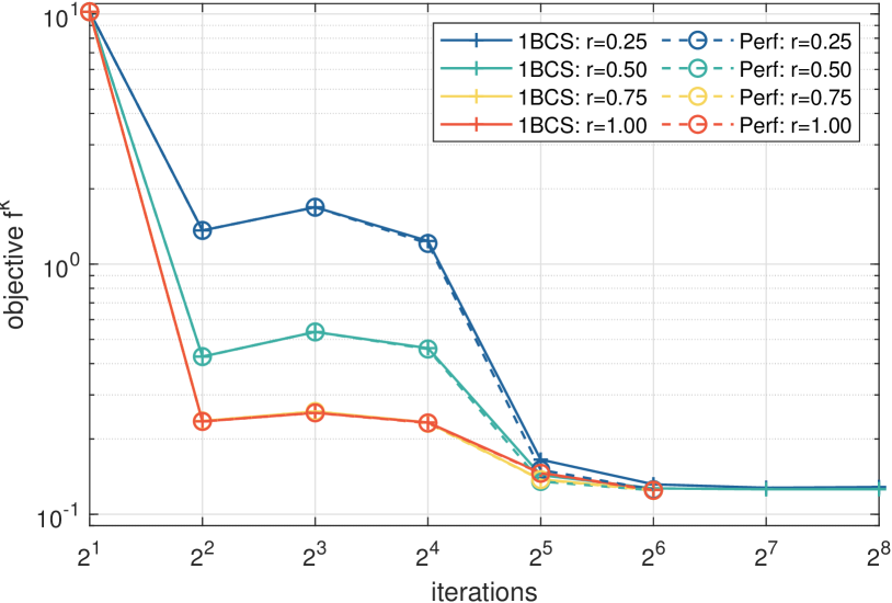
Figure 1: Convergence performance.

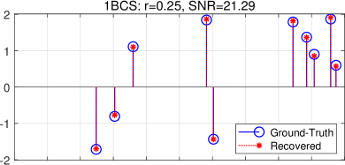
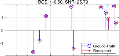
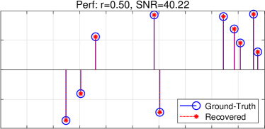
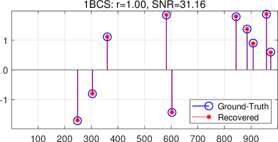
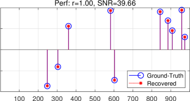
Figure 2: Recovery results.

TABLE I: Numerical comparison.

	$r=0.25$			$r=0.50$			$r=0.75$			$r=1.00$
	1BCS	Perf		1BCS	Perf		1BCS	Perf		1BCS	Perf
SNR	21.29	37.78		25.79	40.22		30.16	39.81		31.16	39.66
Time	18.36	0.798		24.26	0.645		13.11	0.658		16.58	0.786
Iter.	215	59		160	38		60	39		59	55

IV Conclusion

The proposed algorithm integrates three main innovations. The usage of 1BCS enables efficient communication, calculating complex items at specific steps reduces the computational complexity, and selecting partial neighbour nodes to take part in the training eliminates the stragglers’ effect and confronts the challenges of imperfect communication links. Therefore, the algorithm showcases significant potential of solving some practical applications, such as resource allocation, deserving future research. Additionally, exploring its convergence properties and comparing it with other leading algorithms are also promising topics for investigation.

References

- [1] J. Konečnỳ, B. McMahan, and D. Ramage, “Federated optimization: Distributed optimization beyond the datacenter,” arXiv preprint arXiv:1511.03575, 2015.
- [2] J. Konečnỳ, H. B. McMahan, D. Ramage, and P. Richtárik, “Federated optimization: Distributed machine learning for on-device intelligence,” arXiv preprint arXiv:1610.02527, 2016.
- [3] S. Samarakoon, M. Bennis, W. Saad, and M. Debbah, “Distributed federated learning for ultra-reliable low-latency vehicular communications,” IEEE Trans. Commun., vol. 68, no. 2, pp. 1146–1159, 2019.
- [4] S. R. Pokhrel, “Federated learning meets blockchain at 6g edge: A drone-assisted networking for disaster response,” in ACM MobiCom, 2020, pp. 49–54.
- [5] A. M. Elbir, B. Soner, and S. Coleri, “Federated learning in vehicular networks,” arXiv preprint arXiv:2006.01412, 2020.
- [6] J. Posner, L. Tseng, M. Aloqaily, and Y. Jararweh, “Federated learning in vehicular networks: opportunities and solutions,” IEEE Netw., vol. 35, no. 2, pp. 152–159, 2021.
- [7] N. Rieke, J. Hancox, W. Li, F. Milletari, H. R. Roth, S. Albarqouni, S. Bakas, M. N. Galtier, B. A. Landman, K. Maier-Hein et al., “The future of digital health with federated learning,” NPJ Digit. Med., vol. 3, no. 1, pp. 1–7, 2020.
- [8] Y. Mao, C. You, J. Zhang, K. Huang, and K. B. Letaief, “A survey on mobile edge computing: The communication perspective,” IEEE Commun. Surv. Tutor., vol. 19, no. 4, pp. 2322–2358, 2017.
- [9] S. Zhou and G. Y. Li, “Communication-efficient ADMM-based federated learning,” arXiv preprint arXiv:2110.15318, 2021.
- [10] P. Kairouz, H. B. McMahan, B. Avent, A. Bellet, M. Bennis, A. N. Bhagoji, K. Bonawitz, Z. Charles, G. Cormode, R. Cummings et al., “Advances and open problems in federated learning,” Found. Trends Mach. Learn., vol. 14, no. 1-2, pp. 1–210, 2019.
- [11] T. Li, A. K. Sahu, A. Talwalkar, and V. Smith, “Federated learning: Challenges, methods, and future directions,” IEEE Signal Process. Mag., vol. 37, no. 3, pp. 50–60, 2020.
- [12] Z. Qin, G. Y. Li, and H. Ye, “Federated learning and wireless communications,” IEEE Wirel. Commun., 2021.
- [13] X. Lian, C. Zhang, H. Zhang, C.-J. Hsieh, W. Zhang, and J. Liu, “Can decentralized algorithms outperform centralized algorithms? a case study for decentralized parallel stochastic gradient descent,” Adv. Neural Inf. Process., vol. 30, 2017.
- [14] H. Tang, S. Gan, C. Zhang, T. Zhang, and J. Liu, “Communication compression for decentralized training,” Adv. Neural Inf. Process., vol. 31, 2018.
- [15] A. Koloskova, S. Stich, and M. Jaggi, “Decentralized stochastic optimization and gossip algorithms with compressed communication,” in ICML, 2019, pp. 3478–3487.
- [16] A. Koloskova, T. Lin, S. U. Stich, and M. Jaggi, “Decentralized deep learning with arbitrary communication compression,” in ICLR, 2020.
- [17] A. Lalitha, S. Shekhar, T. Javidi, and F. Koushanfar, “Fully decentralized federated learning,” in NeurIPS, vol. 2, 2018.
- [18] C. Pappas, D. Chatzopoulos, S. Lalis, and M. Vavalis, “Ipls: A framework for decentralized federated learning,” in 2021 IFIP Netw. Conf. IEEE, 2021, pp. 1–6.
- [19] H. Ye, L. Liang, and G. Y. Li, “Decentralized federated learning with unreliable communications,” IEEE J. Sel. Top. Signal Process., vol. 16, no. 3, pp. 487–500, 2022.
- [20] Z. Tang, S. Shi, B. Li, and X. Chu, “Gossipfl: A decentralized federated learning framework with sparsified and adaptive communication,” IEEE Trans. Parallel Distrib. Syst., vol. 34, no. 3, pp. 909–922, 2022.
- [21] J. Wang, A. K. Sahu, Z. Yang, G. Joshi, and S. Kar, “MATCHA: Speeding up decentralized SGD via matching decomposition sampling,” in 2019 Sixth Indian Cont. Conf. IEEE, 2019, pp. 299–300.
- [22] I. Hegedűs, G. Danner, and M. Jelasity, “Gossip learning as a decentralized alternative to federated learning,” in Int. Fed. Conf. Dist. Comput. Tech. Springer, 2019, pp. 74–90.
- [23] C. Li, G. Li, and P. K. Varshney, “Decentralized federated learning via mutual knowledge transfer,” IEEE Internet Things J., vol. 9, no. 2, pp. 1136–1147, 2021.
- [24] I. Hegedűs, G. Danner, and M. Jelasity, “Decentralized learning works: An empirical comparison of gossip learning and federated learning,” J. Parallel Distrib. Comput., vol. 148, pp. 109–124, 2021.
- [25] W. Liu, L. Chen, and W. Zhang, “Decentralized federated learning: Balancing communication and computing costs,” IEEE Trans. Signal Inf. Process. Netw., vol. 8, pp. 131–143, 2022.
- [26] S. Kalra, J. Wen, J. C. Cresswell, M. Volkovs, and H. Tizhoosh, “Decentralized federated learning through proxy model sharing,” Nat. Commun., vol. 14, no. 1, p. 2899, 2023.
- [27] P. T. Boufounos and R. G. Baraniuk, “1-bit compressive sensing,” in 42nd Annu. Conf. Inf. Sci. Syst. IEEE, 2008, pp. 16–21.
- [28] S. Zhou, Z. Luo, N. Xiu, and G. Y. Li, “Computing one-bit compressive sensing via double-sparsity constrained optimization,” IEEE Trans. Signal Process., vol. 70, pp. 1593–1608, 2022.
- [29] L. Jacques, J. N. Laska, P. T. Boufounos, and R. G. Baraniuk, “Robust 1-bit compressive sensing via binary stable embeddings of sparse vectors,” IEEE Trans. Inf. Theory, vol. 59, no. 4, pp. 2082–2102, 2013.
- [30] S. Zheng, Q. Meng, T. Wang, W. Chen, N. Yu, Z.-M. Ma, and T.-Y. Liu, “Asynchronous stochastic gradient descent with delay compensation,” in ICML, vol. 7, 2017, p. 4120–4129.
- [31] H. Yu, S. Yang, and S. Zhu, “Parallel restarted SGD with faster convergence and less communication: Demystifying why model averaging works for deep learning,” AAAI, vol. 33, no. 1, pp. 5693–5700, 2019.
- [32] J. Wang and G. Joshi, “Cooperative SGD: A unified framework for the design and analysis of local-update SGD algorithms,” J. Mach. Learn. Res., vol. 22, no. 213, pp. 1–50, 2021.
- [33] B. McMahan, E. Moore, D. Ramage, S. Hampson, and B. A. y Arcas, “Communication-efficient learning of deep networks from decentralized data,” in Artif. Intel. Stat. PMLR, 2017, pp. 1273–1282.
- [34] X. Li, K. Huang, W. Yang, S. Wang, and Z. Zhang, “On the convergence of FedAvg on non-iid data,” in ICLR, 2020.
- [35] T. Li, A. K. Sahu, M. Zaheer, M. Sanjabi, A. Talwalkar, and V. Smith, “Federated optimization in heterogeneous networks,” MLSys, vol. 2, pp. 429–450, 2020.
- [36] S. Zhou and G. Y. Li, “FedGiA: An efficient hybrid algorithm for federated learning,” IEEE Trans. Signal Process., vol. 71, pp. 1493–1508, 2023.
- [37] Y. Li, T.-H. Chang, and C.-Y. Chi, “Secure federated averaging algorithm with differential privacy,” in 2020 IEEE 30th Int. Workshop Mach. Learn. Signal Process. IEEE, 2020, pp. 1–6.
- [38] S. Zhou and G. Y. Li, “Federated learning via inexact ADMM,” IEEE Trans. Pattern Anal. Mach. Intell., vol. 45, pp. 9699–9708, 2023.
- [39] Y. Li, S. Wang, T.-H. Chang, and C.-Y. Chi, “Federated stochastic primal-dual learning with differential privacy,” arXiv preprint arXiv:2204.12284, 2022.