The nuclear liquid-gas transition in QCD

Abstract

We estimate the nuclear saturation density and the binding energy in a nuclear liquid from precision data on the coupling of the four-quark scattering vertex in the vector channel, computed within functional QCD. We show that this coupling is directly related to the density-density potential and the latter is used for the estimates. In a first qualitative computation we find a saturation density of 0.2 fm^-3 and an upper bound for the binding energy of 21.5 MeV, in agreement with the empirical values of 0.16 fm^-3 and 16 MeV, respectively. We also use the scattering vertex for constructing an emergent low-energy effective theory for the liquid gas transition from QCD correlation function, whose coupling parameters can be determined within QCD. As a first consistency check of this construction we estimate the in-medium reduction of the nucleon pole mass.

I Introduction

One of the few experimentally accessible aspects of the low-temperature phase structure of strongly interacting matter is the liquid-gas transition in symmetric nuclear matter [1]. It is a first-order phase transition at which nucleons pile up into a nuclear liquid, and nuclei can be thought of as droplets of this liquid. The binding energy in the infinite nuclear liquid is known to be $16\text{\,}\mathrm{MeV}$ at the saturation density $n_{b}=n_{b}^{\text{(sat)}}\simeq 0.16{\;\text{fm}^{-3}}$ at vanishing temperature. In the nuclear experiment finite-size effects are crucial but some signatures have been confirmed; see [2] for a summary of measured observables.

This phenomenon is less understood from first principles theory, i.e., quantum chromodynamics (QCD), as it combines a couple of challenging problems of strongly correlated low-energy QCD. The understanding of the liquid-gas transition necessitates the determination of the nucleon pole mass $m_{b}$ and the excitation energy per nucleon $E/A$ as a function of the baryon density $n_{b}$. The minimum location and the depth of $E/A$ give the saturation density $n_{b}^{\text{(sat)}}$ and the binding energy $\epsilon_{b}$, respectively. The determination of the nucleon mass in the vacuum has been achieved from Dyson-Schwinger (DSE)–Bethe-Salpeter (BSE)–Faddeev equations; see [3] for a recent review. This result has been reproduced within lattice-QCD simulations; see [4] for a review. As for the other two observables, the saturation density $n_{b}^{\text{(sat)}}$, and the binding energy $\epsilon_{b}$, the energy density functional has not been derived yet from first principles QCD except in special regimes; see e.g. [5, 6] for lattice-QCD approaches to nuclear matter at strong coupling.

As long as the baryon density is close to the saturation density, the protocol of ab initio calculations of QCD within a derivative expansion ought to be valid. In this way the nuclear equation of state (EOS) has been estimated for symmetric and asymmetric nuclear matter; see [7] for a review of pioneering works. The chiral approach continues up to next-to-next-to-next-leading order (N³LO) including many-body interactions [8], which has been applied to constrain properties of neutron stars [9]. Although the chiral effective theory has predictive power near the saturation density, the validity region is limited below the baryon density $1.2$-$1.5\,n_{b}^{\text{(sat)}}$. Thus, it is desirable to complement our understanding of the liquid-gas transition of nuclear matter with microscopic descriptions with a more direct connection to QCD. In this direction a hybrid method using two complementary approaches has been discussed; see [10].

In the present work we demonstrate that the four-quark scattering amplitude $\lambda_{\omega}(\vec{p})$ in the density channel sets the relevant scale for the liquid-gas transition. This scattering amplitude has been computed in a first principles functional renormalisation group approach to QCD [11, 12, 13], The amplitude $\lambda_{\omega}(\vec{p})$ or its Fourier transform in position space exhibits a repulsive short-distance part for $r\to 0$ and an attractive long-distance part for $r\to\infty$. We translate $\lambda_{\omega}(\vec{p})$ into a potential energy of density correlations, and the stable point leads to a direct estimate of the saturation density as well as the binding energy. Interestingly, $n_{b}^{\text{(sat)}}$ and $\epsilon_{b}$ deduced from the potential energy turn out to be compatible with the empirical values.

The first principles QCD correlation functions in [11, 14, 12, 13, 15] can also be used to compute the emergent low-energy effective theory of baryons, mesons, and quarks along the lines set up in [16]. This low-energy effective theory of QCD governs the dynamics of the liquid-gas transition of nuclear matter, and unlike conventional model studies its parameters are fixed by the QCD results in [11, 12, 13]. For instance, $\lambda_{\omega}$ has been a fitting parameter in phenomenological approaches such as quantum hadrodynamics (QHD) by Serot and Walecka [17]. The covariantly extended formalism of relativistic mean-field nuclear calculations still needs this parameter $\lambda_{\omega}$, which is usually inferred from the intrinsic property of the $\omega$ meson. In contradistinction, in the present work we utilise the momentum dependence of $\lambda_{\omega}(\vec{p})$ computed in QCD. This momentum dependence encodes rich physics, which is not fully taken into account in simple mean-field calculations. We note that this momentum dependence is reminiscent of the effective nuclear potential, such as the Skyrme interaction and the Gogny interaction, that is density-dependent, for a recent review, see [18]. This can be understood from the correspondence between the density and the Fermi momentum, or that between the characteristic inter-particle distance at a certain density and the momentum scale. In this sense first principles data on $\lambda_{\omega}(\vec{p})$ sheds light on the density-dependent phenomenological potential in nuclear physics.

II The nuclear liquid from density-density correlations

In this section we put forward an approach for computing the binding energy $\epsilon_{{b}}$ in a nuclear liquid at the saturation density $n_{b}^{\text{(sat)}}$ from quark and baryon correlation functions in first principles QCD. These observables are encoded in the static potential between nucleons or the density-density potential $V_{b}(r)$ in the liquid at a distance $r$, and its estimate from QCD correlation functions is presented in Figure 1. In particular, the density is obtained from the location $d_{b}$ of the minimum of the potential, as $d_{b}$ is related to the distance between nucleons in the nuclear liquid. The depth of the potential at $d_{b}$ offers an estimate for the binding energy $\epsilon_{{b}}$.

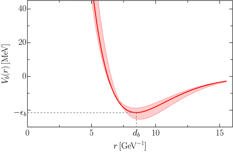
Figure 1: Static density-density potential $V_{b}(r)$ 12 as a function of distance $r$ in the nuclear liquid, computed from QCD correlation functions in [13]. We identify the position of the minimum of the potential, $d_{b}$, with a typical length scale for the distance between nucleons in the nuclear liquid, and the depth of the minimum with the binding energy $\epsilon_{{b}}$. These are found to be $d_{b}\approx$8.5(3)\text{\,}\mathrm{G}\mathrm{eV}^{-1}$$ and $\epsilon_{b}\approx$21(5)\text{\,}\mathrm{M}\mathrm{e}\mathrm{V}$$.

II.1 Density-density potential in the nuclear liquid

We proceed with extracting the density-density potential $V_{b}(r)$ in the nuclear liquid from density-density correlations in first principles QCD: the static baryon density $n_{b}(\vec{x})$ with $\partial_{t}n_{b}(x)=0$ describes a number of nucleons in ${\cal N}_{x}$,

$$\int_{\vec{x}\in{\cal N}_{x}}n_{b}(x)\,,$$ (1)

where ${\cal N}_{x}$ is some infinitesimal neighbourhood of $\vec{x}$. In the present spatially homogeneous situation, 1 is directly related to the average density, the first density moment, computed by a $\mu_{b}$-derivative of the grand potential $\Omega$ in QCD,

$$n_{b}=\frac{1}{{\cal V}_{4}}\int_{x}\langle\hat{n}_{b}(x)\rangle=-\frac{1}{{\cal V}_{4}}\frac{\partial\Omega}{\partial\mu_{{b}}}\,,$$ (2)

where we have divided out the space-time volume ${\cal V}_{4}$. The grand potential $\Omega$ is nothing but the effective action $\Gamma_{\textrm{QCD}}$ of QCD, evaluated on the equations of motion (EoM), i.e.,

$$\Omega=\left.\Gamma_{\textrm{QCD}}\right|_{\textrm{EoM}}\,.$$ (3)

For $\mu_{b}<\mu_{b}^{\textrm{os}}$, the density is vanishing. Here, $\mu_{b}^{\textrm{os}}$ is the onset chemical potential. For larger baryon chemical potentials, $\mu_{b}>\mu_{b}^{\textrm{os}}$, the density is non-vanishing. At the onset chemical potential for symmetric nuclear matter, the density jumps to the saturation density

$$n_{b}^{\text{(sat)}}=n_{b}(\mu_{{b}}^{\text{(os)}})\neq 0\,,$$ (4)

at the first order nuclear liquid-gas transition. In the present work we estimate the size of $n_{b}^{\text{(sat)}}$ from $V_{b}(r)$, but in Section III we also discuss its derivation from effective field theory considerations.

The two-body potential $V_{b}(r)$ is the second static moment of local density fluctuations in position space and is given by

$$\int_{x,y}\langle\hat{n}_{b}(x)\hat{n}_{b}(y)\rangle_{\mathrm{c}}=\frac{\partial^{2}\Omega}{\partial\mu_{{b}}^{2}}\,,$$ (5)

where the subscript c indicates that the second derivative of the grand potential w.r.t. the baryon chemical potential provides the connected part of the density-density correlation,

$$\langle\hat{n}_{b}(x)\hat{n}_{b}(y)\rangle_{\mathrm{c}}=\langle\hat{n}_{b}(\vec{x})\hat{n}_{b}(\vec{y})\rangle-n_{b}(\vec{x})n_{b}(\vec{y})\,.$$ (6)

The integrand 6 of 5 comprises both observables under investigation: $n_{b}^{\text{(sat)}}$ and $\epsilon_{b}$.

It is left to compute the density correlation 5 from correlation functions in first principles QCD. While 5 is the integrated correlation, we are interested in the local one, 6,

$$\langle\hat{n}_{b}(x)\hat{n}_{b}(y)\rangle_{c}=\frac{\delta^{2}\Gamma_{\textrm{QCD}}}{\delta\mu_{b}(x)\delta\mu_{b}(y)}\,,$$ (7)

evaluated for a static situation. Note that in contrast to 5, the derivatives in 7 are functional derivatives, which compensate for the two spacetime integrations in 5 by giving rise to delta distributions.

The respective term in the QCD effective action, formulated in terms of the baryon density, is given by

$$\Gamma_{n_{b}n_{b}}=-\int_{x,y}n_{b}(x)\,\lambda_{n_{b}n_{b}}(x-y)\,n_{b}(y)\,,$$ (8)

with the interaction strength $\lambda_{n_{b}n_{b}}(x-y)$. We emphasise that 8 strictly holds in a density functional approach to QCD, where the baryon or quark density has been introduced as a dynamical variable. This is tantamount to introducing a dynamical field for the vector mode $\omega_{0}$ via dynamical hadronisation as discussed in [16].

The static equal time part of 8 is obtained for $\partial_{t}n_{b}(t,\vec{x})=0$. Inserting such a static density distribution into 8 leads us to

$$\frac{1}{T}\Gamma_{n_{b}n_{b}}=-\int_{\vec{x},\vec{y}}n_{b}(\vec{x})V_{b}(r)n_{b}(\vec{y})\,,$$ (9)

where the potential $V_{b}(r)$ is nothing but the dressing factor of the density-density term and $r$ is the distance between the density locations,

$$\qquad r=\|\vec{x}-\vec{y}\|\,.$$ (10)

In 9 we have divided out the time extent $T$ with the space-time volume ${\cal V}_{4}=T\,{\cal V}_{3}$, where ${\cal V}_{3}$ is the spatial volume. The density-density potential $V_{b}(r)$ in 9 is simply given by the static part of the coupling $\lambda_{n_{b}n_{b}}$,

$$V_{b}(r)=\int_{-T/2}^{T/2}dt\,\lambda_{n_{b}n_{b}}(t,r)\,.$$ (11)

The potential $V_{b}(r)$ in 11 can be obtained as Fourier transform from momentum dependent data for $\lambda_{n_{b}n_{b}}(p)$ via

$$V_{b}(r)\simeq\int\frac{\textrm{d}^{3}p}{(2\pi)^{3}}V_{b}(\vec{p})\,e^{\text{i}\vec{p}(\vec{x}-\vec{y})}\,,$$ (12a)

where we identify

$$V_{b}(\vec{p})=\lambda_{n_{b}n_{b}}(p_{0}=0,\vec{p})\,.$$ (12b)

In Figure 1, we display our estimate for the potential $V_{b}(r)$ 12 of static density-density correlations obtained from fundamental QCD correlation functions in [13]. The distance $r=d_{b}$ of its minimum is the distance of “cells” in the gas or fluid and hence is directly related to the density. In turn, its depth $-V_{b}(d_{b})$ provides an estimate for the binding energy.

II.2 Density-density correlations from QCD

In the present work we utilise QCD correlation functions from [13], computed in terms of quark, gluons and mesons, and hence we rewrite 8 as a correlation of the quark-density with $n_{q}=3n_{b}$,

$$\Gamma_{n_{b}n_{b}}=-\frac{1}{9}\int_{x,y}n_{q}(x)\,\lambda_{n_{b}n_{b}}(x-y)\,n_{q}(y)\,.$$ (13)

Hence, the coupling strength of the quark density is a ninth of that of the baryon density. The density operator $n_{q}$ is proportional to the quark bilinear $\bar{q}\gamma_{0}q$, but also features the wave function $Z_{q}(p)$ of the quark,

$$n_{q}\propto Z_{q}\bar{q}\gamma_{0}q\,.$$ (14)

The wave function is the “dressing” of the full kinetic term of the QCD effective action and reads

$$\Gamma_{q,\textrm{kin}}=\int_{p}Z_{q}(p)\bar{q}(p)\bigg{[}\text{i}p\hskip 0.42677pt\hbox to0.0pt{\hss/}\hskip 0.42677pt-\gamma_{0}\mu_{q}+M_{q}(p)\bigg{]}q(-p)\,,$$ (15)

where we have dropped a further splitting of the tensor structure in the presence of the chemical potential, which singles out the rest frame. The wave function $Z_{q}(p)$ absorbs the RG-scaling of the quark fields, leaving us with an RG-invariant mass function $M_{q}(p)$. More generally, all fields in the effective action have to be accompanied by their respective wave functions $Z^{1/2}(p)$, leaving us with RG-invariant dressings such as $M_{q}$.

The baryon density-density contribution to the effective action 13 in momentum space takes the form

$$\Gamma_{n_{b}n_{b}}=-\frac{1}{9}\int_{p}n_{q}(-p)\,\lambda_{n_{b}n_{b}}(p)\,n_{q}(p)\,.$$ (16)

Taking into account 14, in the lowest order approximation the density in momentum space $n_{q}(p)$ takes the form

$$n_{q}(p)\simeq\int_{l}Z^{1/2}_{q}(l-p)Z^{1/2}_{q}(p)\bar{q}(l-p)\gamma_{0}q(p)\,.$$ (17)

Equation 17 holds in the mean field or Gaußian approximation, and its corrections contain higher order terms of the density quark bilinear and further higher order terms in the quarks and anti-quarks. This complete relation has been exhaustively studied at the example of the scalar-pseudoscalar channel: in [13] and other works, the scalar-pseudoscalar channel has been treated within dynamical hadronisation, and the emergent scalar $\sigma$-mode and pions $\bm{\pi}^{T}=(\pi_{1},\pi_{2},\pi_{3})$ have been introduced. To the lowest order, this amounts to identifying e.g. $\sigma(x)\propto\bar{q}(x)q(x)$ by the equations of motion of $\sigma$. However, at the full quantum level higher order terms in the bilinear $\bar{q}(x)q(x)$ (and others) enter via the full effective potential $V_{\textrm{eff}}((\sigma^{2}+\bm{\pi}^{2})/2)$. These terms are relevant for the non-trivial pion dynamics in the infrared that generates chiral perturbation theory.

In contradistinction to the important dynamics in the pseudoscalar channel, it has been shown in [16], that the identification 17 holds true for $\mu_{q}\leq\mu^{\textrm{(os)}}_{q}$. Note that the analysis in [16] was done in terms of $\omega_{0}$, the zero component of the vector iso-scalar channel field $\omega_{\mu}$. In the following we assume the approximation 17 to also hold for chemical potentials $\mu_{q}\gtrsim\mu^{\textrm{(os)}}_{q}$ close the onset chemical potential.

In conclusion, we can directly use the results in [13] for the density channel of the four-quark scattering terms,

$$\Gamma_{n_{q}n_{q}}\simeq \,-\frac{1}{4}\int_{p}\lambda_{\omega}(p_{1},p_{2},p_{3})$$

$$\hskip 28.45274pt\times\left[\bar{q}(p_{1})\gamma_{0}q(p_{2})\right]\left[\bar{q}(p_{3})\gamma_{0}q(p_{4})\right]\,,$$ (18)

with $p=(p_{1},p_{2},p_{3})$ and $p_{4}=-(p_{1}+p_{2}+p_{3})$. In 18, $\lambda_{\omega}$ is a combination of couplings $\lambda^{(V\pm A)}$ to vector–axial-vector four-quark operators as used in [11] and [13],

$$\lambda_{\omega}=\lambda^{(V+A)}+\lambda^{(V-A)}\,.$$ (19)

In [13], the vertex dressing $\lambda_{\omega}(p_{1},p_{2},p_{3})$ has been evaluated at the momentum $p$ for the anti-quarks and $-p$ for the quarks,

$$\lambda_{\omega}(p)=\lambda_{\omega}(p,-p,p)\,.$$ (20)

This is precisely the momentum configuration of the quark number current $n_{q}$ 14, that couples to the chemical potential in 15. Hence, within a qualitative estimate we identify the RG-invariant coupling $\lambda_{n_{b}n_{b}}(p)$ with the coupling in the vector channel (up to a factor 9/4),

$$\lambda_{n_{b}n_{b}}(p)\approx\frac{9}{4}\bar{\lambda}_{\omega}(p)\,,\qquad\bar{\lambda}_{\omega}(p)=\frac{\lambda_{\omega}(p)}{Z_{q}(p)^{2}}\,,$$ (21)

as the RG-invariant coupling between two density operators 15. In 21 we have also introduced the RG-invariant vector coupling $\bar{\lambda}_{\omega}$, deduced from the vertex dressing $\lambda_{\omega}$ and the quark wave function $Z_{q}$. We emphasise that the vertex dressing $\lambda_{\omega}$ of the four-quark correlation function is not an RG-invariant quantity.

These preparations allow us to compute $V_{b}(r)$ as the Fourier transform of the RG-invariant four-quark scattering coupling 12. The latter momentum space potential is displayed in Figure 2, where we exploited that the data of [13] is obtained in the vacuum, and hence

$$\lambda_{\omega}(p_{0}=0,\vec{p})=\lambda_{\omega}(p^{2}=\vec{p}^{\,2})\,,$$ (22)

where $p^{2}=p_{0}^{2}+\vec{p}^{\,2}$ in our convention. The Fourier transform of the momentum space potential leads to Figure 1. Hence, the error estimates in Figures 2 and 1 are that of $\lambda_{\omega}$ in [13], translated to the respective quantities here.

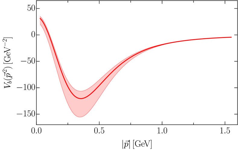
Figure 2: Static density-density potential in momentum space, see 12 and 21, using the $\bar{\lambda}_{\omega}$-data of [13]. A fit of $\bar{\lambda}_{\omega}$ is provided in Table 1 in Appendix A. In the argument of $V_{b}(\vec{p}^{\,2})$ we made apparent that since the input data is obtained in the vacuum, no rest frame is singled out. The value of the potential in the minimum, 53, is used for an estimate of the nucleon mass in the liquid, see 54.

II.3 The nuclear liquid

We are now in the position to provide estimates for the onset density as well as the nucleon binding energy from first principles QCD. A last step concerns the total error estimate. Apart from the errors already mentioned there is a further one originating in the translation of the two-flavor scales to the physical case. In both cases the system is tuned to a pion mass $m_{\pi}\approx$140\text{\,}\mathrm{MeV}$$. The off-shell dynamics of the strange quark influences the momentum dependence of $\lambda_{\omega}$, as it does the size and momentum-dependence of the light constituent quark mass

$$M_{l}=M_{l}(0)\,,$$ (23)

see e.g. [15]. This leads to a rescaling factor

$$\gamma\approx\frac{M_{l}^{(2+1)}}{M_{l}^{(2)}}=0.92\,,$$ (24)

for momenta and $1/\gamma$ for distances of some observables, leaving us with roughly a further 10% error. Our combined conservative error estimate sums up to 25%, where a further 5% span was added.

The effective nucleon potential $V_{b}$ in 12, depicted in Figure 1, clearly displays a minimum at a distance $d_{b}$ with

$$d_{b}=$8.5(21)\text{\,}\mathrm{G}\mathrm{eV}^{-1}$\approx$1.67(42)\text{\,}\mathrm{f}\mathrm{m}$\,,$$ (25)

with the 25% error estimate. This allows us to provide an upper bound for the onset density: we estimate it by a cubic lattice density $n_{b}\sim 1/d_{b}^{3}$, which rather is the density of a solid state system. We obtain

$$n^{\text{(sat)}}_{b}=$0.21(16)\text{\,}\textrm{fm}^{-3}$\,,$$ (26)

where we used Gaußian error propagation of the error on $d_{b}$ in 25. This QCD-based estimate is in good agreement with the measured nuclear density of $n^{\textrm{exp}}_{b}=$0.16\text{\,}\;\text{fm}^{-3}$$. The potential $V_{b}$ also allows for an estimate or rather upper bound of the nucleon binding energy by the depth of the potential. This leads us to

$$\epsilon_{b}\lesssim$21(5)\text{\,}\mathrm{M}\mathrm{e}\mathrm{V}$\,.$$ (27)

This bound is in good agreement with the experimentally established literature value for the nuclear binding energy of $\epsilon^{\textrm{exp}}_{b}=$16\text{\,}\mathrm{MeV}$$ per nucleon.

In summary, the values of the estimates 26 and 27 are very promising and support the validity of the current first principles approach. However, the large errors have to be systematically reduced in future applications, and we envisage work in two obvious directions: First, the density can be extracted from the full form of density-density potential $V_{b}$, a corresponding fit is provided in Appendix A. Second, the estimates can be improved by a direct computation of the nucleon-nucleon potential, which can be done in terms of the functional renormalisation group approach with emergent hadrons and is described in Section III. However, both extensions are beyond the scope of the present work.

III The nuclear liquid from emergent hadrons

The results in Section II for the saturation density and the binding energy in a nuclear liquid have been derived from the density-density term in the QCD effective action 9, whose coupling was inferred from the four-quark scattering in the density channel of QCD. It is therefore suggestive to introduce the density mode and other emergent composites as dynamical degrees of freedom, hence facilitating the direct access to observables in low-energy QCD. This simple idea has been used very successfully since many decades within low-energy effective theories of QCD. If embedded directly in QCD, this finally allows for a direct computation of the nucleon-nucleon potential and hence gives a direct access to the physics of the liquid gas transition also beyond the few but crucial observables estimated here.

In the functional renormalisation group approach these low-energy effective theories of QCD and the respective composite degrees of freedom emerge dynamically within first principles QCD. This allows us to determine the couplings such as $\lambda_{\omega}$ in the low-energy effective theories from that of first principle QCD correlation functions.

III.1 Low-Energy effective theory with emergent vector mesons

So far this formulation has mostly been used for the scalar-pseudoscalar channel in QCD [19, 20, 11, 14, 12, 13, 15, 16] and the vector channel [12]; for reviews see [21, 22]. In [16] the general set-up with emergent composites has been described, including also baryons. For the four-quark interactions this amounts to a scale-dependent Hubbard-Stratonovich transformation whose scale-dependence generates also higher order terms and makes the transformation exact. For the present purpose this is done by rewriting the four-quark interaction term 18 in the density channel in terms of the density mode $\omega_{0}$. This leads us to

$$\Gamma_{n_{q}n_{q}}\simeq \Biggl{[}-\int_{p}\bar{q}(-p)\gamma_{0}\left(\frac{h_{\omega}(p)}{2}\omega_{0}\right)\,q(p)$$ (28)

$$+\frac{1}{2}\int_{p}\,Z_{\omega}(p)\,\omega_{0}(-p)\left[p^{2}+m_{\omega}^{2}\right]\,\omega_{0}(p)\Biggr{]}_{\omega_{0}=\omega_{0}^{\text{EoM}}}\,,$$

with the constant solution of the $\omega_{0}$-equation of motion,

$$\omega^{\text{EoM}}_{0}=\frac{1}{{\cal V}_{4}}\int_{p}\frac{1}{Z_{\omega}(p)}\frac{h_{\omega}}{2m_{\omega}^{2}}\bar{q}(-p)\gamma_{0}q(p)\,.$$ (29)

Here, ${\cal V}_{4}$ is the space-time volume and the four-quark coupling and the Yukawa coupling are related by

$$\bar{\lambda}_{\omega}=\frac{\bar{h}_{\omega}^{2}}{2m_{\omega}^{2}}\quad\text{with}\quad\bar{h}_{\omega}=\frac{h_{\omega}}{Z^{1/2}_{\omega}Z_{q}}\,.$$ (30)

In 30, $\bar{\lambda}_{\omega}$ is the RG-invariant coupling 21 in the density channel. Evidently, $\bar{h}_{\omega}$ is the RG-invariant vertex coupling between the density mode $\omega_{0}$ and the quarks derived from the vertex dressing $\lambda_{\omega}$, while $m_{\omega}$ is the mass scale of the density mode $\omega_{0}$.

We emphasise that $\omega_{0}$ specifically refers to the density mode. The $\omega$ vector meson is a subleading four quark tensor structure in the density channel and the temporal component is not a propagating mode with physical polarisation. This subtlety is the reason for the simple kinetic term in III.1 without a transversal structure as commonly used for vector mesons, see in particular [12, 23, 24] for a treatment within the fRG approach and recent developments.

If combining III.1 with the emergent fields in the sigma-pion channel with the respective scalar-pseudoscalar field $\phi=(\sigma,\bm{\pi})$ within the same approximation used here, we arrive at the following approximation for the matter part of the effective action of QCD for low momenta,

$$\Gamma_{\textrm{mat}}= \,\int_{p}Z_{q}(p)\bar{q}(p)\,\Biggl{[}i\,p\hskip 0.42677pt\hbox to0.0pt{\hss/}\hskip 0.42677pt-\gamma_{0}\bar{\mu}_{q}+\frac{h_{\phi}(\rho)}{Z_{q}(p)}\tau\cdot\phi\Biggr{]}\,q(-p)$$

$$+\int_{p}Z_{\phi}(p)\,\phi(p)\,p^{2}\,\phi(-p)+\int_{x}V_{\textrm{eff}}(\rho)$$

$$+\frac{1}{2}\int_{p}\,Z_{\omega}(p)\omega_{0}(-p)\left[p^{2}+m_{\omega}^{2}\right]\,\omega_{0}(p)+\cdots\,,$$ (31)

where $\rho=\tfrac{1}{2}(\sigma^{2}+\bm{\pi}^{2})$ and $\tau\cdot\phi=\tfrac{1}{2}(\sigma+\bm{\sigma}\bm{\pi})$ with the scalar-pseudoscalar field $\phi=(\sigma,\bm{\pi})$. The dots stand for higher order terms, and the shifted chemical potential $\bar{\mu}_{q}$ is given by

$$\bar{\mu}_{q}=\mu_{q}+\frac{h_{\omega}}{2Z_{q}}\omega_{0}\,.$$ (32)

If 31 is evaluated on the equations of motion for $\phi$ and $\omega_{0}$, the effective action $\Gamma_{\textrm{mat}}$ reduces to the kinetic term of the quarks and four-quark scattering terms in the scalar-pseudoscalar and vector channels. The coupling $\bar{\lambda}_{\omega}$ of the latter is given by 30, the coupling $\bar{\lambda}_{\phi}$ of the former by

$$\bar{\lambda}_{\phi}=\frac{\bar{h}_{\phi}^{2}}{2m_{\phi}^{2}}\quad\text{with}\quad\bar{\lambda}_{\phi}=\frac{\lambda_{\phi}}{Z^{2}_{q}},\quad\bar{h}_{\phi}=\frac{h_{\phi}}{Z_{\phi}^{1/2}Z_{q}}\,,$$ (33)

see e.g. [11, 14, 12, 13, 15, 16]. In analogy to 30, the RG-invariant coupling $\bar{h}_{\phi}$ is derived from the vertex dressing $h_{\phi}(\rho)$. The dynamical $\sigma$ and $\bm{\pi}$ fields come with a full effective potential $V_{\textrm{eff}}(\rho)$ that includes all order self-scatterings of these fields.

In turn, it has been shown in [16] that no such potential is generated for sufficiently small $\omega_{0}$ due to the property that is often called the “Silver Blaze” after Sherlock Holmes (see [25]) for sufficiently small $\omega_{0}$ and chemical potentials. This connection is apparent in the first line of 31, where $\omega_{0}$ enters as a shift of the quark chemical potential, see 32. Hence, an $\omega_{0}$-derivative of $\Gamma_{\textrm{mat}}$ can be written in terms of a $\bar{\mu}_{q}$-derivative and the $\omega_{0}$-derivative of the kinetic term of the $\omega_{0}$. This leads us to the following equation of motion for a constant $\omega_{0}$,

$$\left.\frac{\partial\Gamma_{\textrm{mat}}}{\partial\bar{\omega}_{0}}\right|_{\omega_{0}=\omega_{0}^{\textrm{EoM}}}=\frac{\bar{h}_{\omega}}{2}\frac{\partial\Gamma_{\textrm{mat}}}{\partial\mu_{q}}+m_{\omega}^{2}Z^{1/2}_{\omega}\omega^{\textrm{EoM}}_{0}=0\,,$$ (34)

where we have used that the $\bar{\mu}_{q}$-derivative is simply a $\mu_{q}$-derivative. This makes apparent, that the first term on the right hand side is nothing but (minus) the quark density 2, multiplied by $h_{\omega}/2Z_{q}$. Hence, the constant solution of the equation of motion is

$$Z^{1/2}_{\omega}\omega_{0}^{\textrm{\tiny{EoM}}}=\frac{\bar{h}_{\omega}}{2m_{\omega}^{2}}n_{q}\,.$$ (35)

On the equations of motion, 35 vanishes for chemical potentials smaller than the onset chemical potential $\mu_{q}^{\text{(on)}}$. To make the lack of $\omega_{0}$-dependences below onset more apparent, we rewrite the effective action in terms of the shifted and renormalisation group invariant field $\bar{\omega}_{0}$ with

$$\bar{\omega}_{0}=Z_{\omega}^{1/2}\omega_{0}+\frac{2}{\bar{h}_{\omega}}\mu_{q}\,,$$ (36)

where both terms are separately RG-invariant. With 36 we readily obtain

$$\Gamma_{\textrm{mat}}[Z_{\omega}^{1/2}\omega_{0};\mu_{q}]=\Gamma_{\textrm{mat}}[\bar{\omega}_{0};0]-\frac{2m_{\omega}^{2}}{\bar{h}_{\omega}}\bar{\omega}_{0}\mu_{q}+\frac{2m_{\omega}^{2}}{\bar{h}_{\omega}^{2}}\mu_{q}^{2}\,,$$ (37)

where we have only kept the $\bar{\omega}_{0}$- and $\mu_{q}$-arguments of $\Gamma_{\textrm{mat}}$ explicit. In $\Gamma_{\textrm{mat}}[\bar{\omega}_{0};0]$, the field $\bar{\omega}_{0}$ has taken the role of the chemical potential and hence there is no $\bar{\omega}_{0}$-dependence for

$$|\bar{\omega}_{0}|\leq\mu_{q}^{\text{(on)}}\,.$$ (38)

This concludes our proof of the absence of an effective potential for $\bar{\omega}_{0}$ with 38.

On the solution 34 of the EoM, the $\mu_{b}$-derivative of $\Gamma_{\textrm{mat}}$ only hits the explicit $\mu_{b}$-dependence on the right hand side of 37, and we arrive at

$$n_{q}=\frac{2m_{\omega}^{2}}{\bar{h}_{\omega}}\bar{\omega}_{0}^{\textrm{\tiny{EoM}}}-\frac{4m_{\omega}^{2}}{\bar{h}_{\omega}^{2}}\mu_{q}=\frac{2m_{\omega}^{2}}{\bar{h}_{\omega}}Z_{\omega}^{1/2}\omega_{0}^{\textrm{\tiny{EoM}}}\,,$$ (39)

which vanishes for $\omega^{\textrm{EoM}}_{0}=0$. For $\mu_{\textrm{q}}>\mu_{q}^{\text{(on)}}$, the baryon density is non-vanishing. The onset chemical potential is determined by the distance of the first singularity of $M_{q}(p)$ in the complex frequency plane from the Euclidean frequency axis for vanishing spatial momentum. Since the quark does not define an asymptotic state this singularity may in principle be complex. We evaluate the location of this singularity in Appendix C. Finally, we can feed back the solution 39 of the EoM into the shifted chemical potential defined in 32. This leads us to

$$\bar{\mu}_{q}^{\textrm{\tiny{EoM}}}=\mu_{q}+\frac{1}{2}\bar{\lambda}_{\omega}\,n_{q}\,.$$ (40)

On the equations of motion the shifted chemical potential only depends on the RG-invariant four-quark coupling $\bar{\lambda}_{\omega}$ and the quark number density.

III.2 The nuclear binding energy from emergent nucleons

If we reformulate the low-energy effective theory in terms of nucleons, the intricacies due to the complex nature of singularity in the quark propagator are softened by the fact that the nucleon defines an asymptotic state. The respective propagator shows a real pole at the nucleon pole mass, and the computation of the onset chemical potential, the corresponding saturation density and the binding energy as well as further observables is facilitated. Then, the matter part of the effective action is given by

$$\Gamma_{\textrm{mat}}\to\Gamma_{\textrm{mat}}+\Gamma_{\textrm{nuc}}\,,$$ (41)

with the nucleon term

$$\Gamma_{\textrm{nuc}}$$

$$\approx\int_{p}\,Z_{b}(p)\,\bar{b}(-p)\Biggl{[}i\,p\hskip 0.42677pt\hbox to0.0pt{\hss/}\hskip 0.42677pt+\gamma_{0}\left(\mu_{b}+\frac{h_{b\omega}}{2Z_{n}}\omega_{0}\right)+m_{b}\Biggr{]}b(p)\,,$$ (42)

where $b$ is a baryon field, representing nucleons here, and we have restricted ourselves a constant nucleon mass function $M_{b}(p)=M_{b}$. Note that in this approximation the Euclidean mass $M_{b}$ is identical with the pole mass $m_{b}$ of the nucleon, i.e., $M_{b}=m_{b}$. Moreover, we shall also use a constant wave function renormalisation $Z_{b}\equiv 1$.

It is left to determine the $b-\omega_{0}$ coupling $\bar{h}_{b\omega}$, which is fixed uniquely by the onset condition (that is the Silver Blaze property below the onset),

$$\bar{h}_{b\omega}=3\bar{h}_{\omega}\,,\qquad$$ (43)

as has been shown in [16]. Below the onset all correlation functions are given by

$$\Gamma^{(n)}_{\Phi_{i_{1}}\cdots\Phi_{i_{n}}}({p_{0}}_{1},...,{p_{0}}_{n};\mu_{q})=\Gamma^{(n)}_{\Phi_{i_{1}}\cdots\Phi_{i_{n}}}({\bar{p}}_{0}{}^{\ }_{1},...,{{\bar{p}_{0}}}{}^{\ }_{n};0)\,,$$ (44)

with

$${\bar{p}_{0}}{}^{\ }_{\Phi_{i}}={\bar{p}_{0}}{}^{\ }_{\Phi_{i}}+i\,\alpha_{\Phi_{i}}\mu_{q}\,.$$ (45)

Here, $3\alpha_{\Phi_{i}}$ is the baryon number of the respective field. For clarity, we briefly collect the $\alpha$’s relevant for the present work, quark/anti-quark: $\alpha_{q}=\pm 1$, mesons ($\phi,\omega_{0}$): $\alpha_{\textrm{mes}}=0$, and nucleon/anti-nucleon: $\alpha_{b}=\pm 3$. In the presence of the density mode, the quark chemical potential is shifted by $\omega_{0}$, see 32. Then, 45 depends on $\bar{\mu}_{q}$ instead of $\mu_{q}$. Specifically, for the baryon field we obtain

$$\bar{\mu}_{b}=3\left(\mu_{q}+\frac{\bar{h}_{\omega}}{2}Z_{\omega}^{1/2}\omega_{0}\right)\,,$$ (46)

leading to 43. In summary this amounts to

$$\left.\frac{\partial\Gamma_{\text{mat}}}{\partial\bar{\omega}_{0}}\right|_{\omega_{0}=\omega^{\textrm{\tiny{EoM}}}_{0}}=\frac{3\bar{h}_{\omega}}{2}\frac{\partial\Gamma_{\text{mat}}}{\partial{\mu}_{b}}+m_{\omega}^{2}Z^{1/2}_{\omega}\omega_{0}^{\text{EoM}}=0\,,$$ (47)

see also 34. The $\mu_{b}$-derivative of the effective action is (minus) the nucleon density,

$$n_{b}=-\frac{\partial\Gamma_{\text{mat}}}{\partial{\mu}_{b}}\,,$$ (48)

and we are led to

$$Z_{\omega}^{1/2}\omega^{\textrm{EoM}}_{0}=\frac{3h_{\omega}}{2m_{\omega}^{2}}n_{b}\quad\rightarrow\quad\bar{\mu}_{b}=\mu_{b}+2\lambda_{n_{b}n_{b}}n_{b}\,,$$ (49)

where we have used 21. This is the nucleon analogue of 40. As we emphasise there, $\bar{\mu}_{b}$ does not depend on dynamical hadronisation parameters $m_{\omega},h_{\omega}$ on the EoM. Instead, it only depends on the nucleon density as well as the fundamental four-nucleon scattering coupling $\lambda_{n_{b}n_{b}}$ in the density-channel.

We assume that off-shell fluctuations of the nucleon play no relevant role to describe the onset of nuclear matter. Moreover, the quark part of the density is subleading nature, and we drop it in the following. Then, the density fluctuations are given by

$$\Gamma_{\bar{\mu}_{b}}= \frac{1}{12\pi^{2}}\Biggl{[}{\bar{\mu}_{b}}\left(5m_{b}^{2}-2{\bar{\mu}_{b}}^{2}\right)\sqrt{{\bar{\mu}_{b}}^{2}-m_{b}^{2}}$$

$$+\frac{3}{2}m_{b}^{4}\log\left(\frac{\bar{\mu}_{b}-\sqrt{\bar{\mu}_{b}^{2}-m_{b}^{2}}}{\bar{\mu}_{b}+\sqrt{\bar{\mu}_{b}^{2}-m_{b}^{2}}}\right)\Biggr{]}\theta({\bar{\mu}_{b}}^{2}-m_{b}^{2})\,.$$ (50)

Differentiation with respect to the nucleon chemical potential yields a self-consistency equation for the nuclear density

$$n_{b}^{2}= \,\frac{4}{(3\pi^{2})^{2}}\left({\bar{\mu}_{b}}^{2}-m_{b}^{2}\right)^{3}$$ (51)

with the density-dependent $\bar{\mu}_{b}$ in 49. At the first order phase transition into the nuclear liquid, the effective nucleon mass is expected to jump to a screened, smaller value as a consequence of a jump of the chiral condensate $\sigma$ to a smaller but still finite value. We arrive at a self-consistency equation for the onset value of the chemical potential $\mu^{\ast}_{b}$ or the nucleon mass $m^{\ast}_{b}$ at saturation density,

$$\mu^{\ast}_{b}=\sqrt{\bigg{(}\frac{3\pi^{2}n^{\text{(sat)}}_{b}}{2}\bigg{)}^{\frac{2}{3}}+\left(m^{\ast}_{b}\right)^{2}}-2\lambda_{n_{b}n_{b}}^{\text{(sat)}}\,n_{b}^{\text{(sat)}}\,.$$ (52)

For the vector coupling $\lambda_{n_{b}n_{b}}^{\text{(sat)}}$ at saturation density we use the minimum of $V_{b}(\vec{p}{\,}^{2})$, depicted in Figure 2, which leads us to

$$\lambda_{n_{b}n_{b}}^{\text{(sat)}}\approx-$120\text{\,}\mathrm{G}\mathrm{e}\mathrm{V}^{-2}$\,,$$ (53)

related to the minimum in position space used to determine the saturation density 26. Moreover, with 27 we get $\mu^{\ast}_{b}=$918\text{\,}\mathrm{MeV}$$, which was obtained by using the vacuum nucleon mass $m_{b}=$939\text{\,}\mathrm{MeV}$$; see Appendix B. With this input the self-consistency equation can be solved numerically for $m_{b}^{\ast}$ as a function of $\mu^{\ast}_{b}$, which leads us to

$$m_{b}^{\ast}\approx 469\,\textrm{MeV}\,,$$ (54)

which shows $50\%$ reduction of the in-medium nucleon mass as compared to the vacuum mass. This estimate is consistent with the conventional calculations within the Dirac-Brueckner-Hartree-Fock theory; see [26] for the relativistic/non-relativistic definitions of the effective masses as functions of the Fermi momentum, [27] for astrophysical implications, [28] for finite-temperature extension, and references therein.

IV Conclusions

We have set-up a first principles approach for computing properties of the nuclear liquid-gas transition in QCD. This approach is based on the computation of the potentials of density correlations in QCD in terms of correlation functions in first principles QCD. Specifically we have related the potential of density-density correlations to the four-quark scattering coupling $\bar{\lambda}_{\omega}$ in the vector channel. From this potential we deduced estimates for the saturation density $n_{b}^{\text{(sat)}}$, see 26, and the binding energy $\epsilon_{b}$, see 27, in Section II, including a systematic error estimate of 25%.

In Section III we have set-up a QCD-assisted low energy effective action, using results in [16], whose vertex dressings and kinetic terms are directly related to correlation functions in first principles QCD. The key ingredient is again given by $\bar{\lambda}_{\omega}$. As a self-consistency check we have computed the nucleon mass in the nuclear liquid, which turned out to be about $50\%$ of the nucleon mass in the vacuum, see 54.

The qualitative results in the present work are very encouraging, and their systematic improvement towards quantitative precision is subject of current work. Updates of the onset baryon chemical potential, the saturation density, the nucleon mass in the liquid as well as other observables await further investigations in the near future.

Appendix A Fit for the four-quark scattering coupling $\bar{\lambda}_{\omega}(p)$ in the vector channel

	$a_{0}$	$a_{1}\left[\textrm{MeV}^{-2}\right]$	$a_{3}\left[\textrm{MeV}^{-2}\right]$	$b_{0}\left[\textrm{MeV}^{2}\right]$	$b_{1}$	$b_{2}\left[\textrm{MeV}^{-2}\right]$	$b_{3}\left[\textrm{MeV}^{-4}\right]$
$\bar{\lambda}_{\omega}$	$1$	$-1.01\cdot 10^{-4}$	$-7.45\cdot 10^{-12}$	$6.51\cdot 10^{5}$	$0.692$	$3.19\cdot 10^{-6}$	$9.18\cdot 10^{-12}$
$\bar{\lambda}_{\omega,\textrm{low}}$	$1$	$-1.76\cdot 10^{-4}$	$-5.98\cdot 10^{-12}$	$9.34\cdot 10^{5}$	$0.975$	$3.66\cdot 10^{-6}$	$1.63\cdot 10^{-11}$
$\bar{\lambda}_{\omega,\textrm{up}}$	$1$	$-0.88\cdot 10^{-4}$	$-5.87\cdot 10^{-12}$	$5.85\cdot 10^{5}$	$0.682$	$3.45\cdot 10^{-6}$	$7.56\cdot 10^{-12}$

Table 1: Fit parameters for the vector coupling $\bar{\lambda}_{\omega}(p)$ as prescribed by 55. Its nucleon analogue $\lambda_{n_{b}n_{b}}(p)=9/4\bar{\lambda}_{\omega}$, see 21, is shown in Figure 2. The upper and lower bounds for the vector coupling are inherited from the original QCD calculation [13].

In this Appendix we provide a quantitative Padé fit of the QCD data of the density channel dressing,

$$\bar{\lambda}_{\omega}(p)=\frac{a_{0}+a_{1}p^{2}+a_{2}p^{4}}{b_{0}+b_{1}p^{2}+b_{2}p^{4}+b_{3}p^{6}}\,.$$ (55)

from which the potential is obtained via 12 and 21. The fit is obtained from a least $\chi^{2}$ optimisation. The fit parameters $a_{i}$ and $b_{i}$ are listed in Table 1.

Appendix B Baryon pole mass

In this Appendix we infer bounds on the nucleon pole mass $m_{b}$ from the position of the first singularity in the complex momentum plane of the quark propagator. The present analysis is based on the QCD approach with emergent composites as set-up in [16], including the density mode $\omega_{0}$, see Section III.

We start by noting that the quark density operator is given by the expectation value of the quark number operator, and hence obeys

$$n_{q}(\mu)\propto\int\frac{d^{4}p}{(2\pi)^{4}}\,\text{tr}\,\gamma_{0}\,G_{q}(p)\,.$$ (56)

The frequency integral in 56 vanishes in the vacuum as $\text{tr}\,\gamma_{0}G_{q}$ is an odd function in frequency space. For small chemical potentials one can always absorb $\bar{\mu}_{q}$ in the frequency integral. However, if $\omega+i\bar{\mu}_{q}$ sweeps over the first singularity in the complex plane, the density starts rising.

The quark propagator has two branches, $G^{-}$ below the onset chemical potential and $G^{+}$ above the onset chemical potential, with $\bar{\mu}_{q}\gtrless\mu_{q}^{\textrm{(on)}}$. It reads

$$G^{\pm}_{q}(p,\mu_{q})=\frac{1}{Z^{\pm}_{q}(\bar{p})}\frac{-i\not{\bar{p}}+M^{\pm}_{q}(\bar{p})}{\bar{p}^{2}+M^{\pm}_{q}{}^{2}(\bar{p})}\,,$$ (57)

with

$$\bar{p}_{\mu}=p_{\mu}+\text{i}\delta_{\mu 0}\bar{\mu}_{q}\,,$$ (58)

and $\bar{\mu}_{q}$ in 32. While $Z^{+}_{q},M^{+}_{q}$ have a genuine $\mu_{q},\omega_{0}$-dependence, $Z^{-}_{q},M^{-}_{q}$ are that in the vacuum due to Silver blaze, and hence

$$G^{-}(p,\mu)=G^{-}(\bar{p},0)\,.$$ (59)

Both propagators carry singularities in the complex frequency plane with the positions $\omega_{\textrm{sing}}$ and we define

$$m^{\pm}_{\textrm{sing}}=\min\big{|}\textrm{Re}(\omega^{\pm}_{\textrm{sing}})\big{|}\,,$$ (60)

with

$$m^{+}_{\textrm{sing}}\leq\mu_{q}^{\textrm{(on)}}\leq m^{-}_{\textrm{sing}}\,.$$ (61)

The onset-chemical potential $\mu_{q}^{\textrm{(on)}}$ is nothing but the combination of the baryon pole mass $m_{b}$ and the binding energy $\epsilon_{b}$,

$$\mu_{q}^{\textrm{(on)}}=\frac{1}{3}\big{(}m_{b}-\epsilon_{b}\big{)}\,,$$ (62)

and in conclusion, $3m_{\text{sing}}^{\pm}+\epsilon_{b}$ are lower and upper estimates of the nucleon pole mass,

$$m^{+}_{\textrm{sing}}<\frac{1}{3}\big{(}m_{b}-\epsilon_{b}\big{)}<m^{-}_{\textrm{sing}}\,.$$ (63)

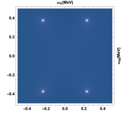
(a)

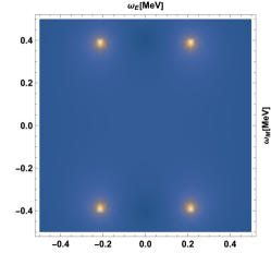
(b)

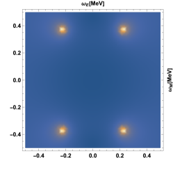
(c)

Figure 3: Padé continuation of $g_{s}$ 67 (left), $g_{s}/Z$ (middle) and $Mg_{s}$ (right) in the complex plane. The distance of the complex conjugate poles to the Euclidean axis yields an upper estimate of the nucleon pole mass with 63, while the deviation of the pole position in the displayed reconstructions yields an error estimate.

In Appendix C, we use numerical results for the Euclidean vacuum quark propagator in two-flavor QCD from [13] to determine the position of the first complex singularity $m^{-}_{\text{sing}}$ of the quark propagator in the below-onset-branch. Due to lack of data in the upper branch, we can only provide an upper estimate for the nucleon mass with 63.

To arrive at this estimate, we need to relate our result for to the two-flavor quark pole mass 69 to the corresponding 2+1-flavor QCD result used in 63. We do this by assuming that the ratio of the pole masses is the same as the ratio of the constituent light quark masses $M_{l}$,

$$\frac{m_{\text{sing}}^{\text{(2)}}}{M_{l}^{\text{(2)}}}=\frac{m_{\text{sing}}^{\text{(2+1)}}}{M^{\text{(2+1)}}}\,,$$ (64)

indicating the number of flavors of the results in the respective superscripts. The reconstruction of the two-flavor pole mass based on the Euclidean two-flavor data in [13] is detailed in Appendix C, its value being $377(9)\text{\,}\mathrm{MeV}$, see 68. The respective two-flavor constituent quark mass from [13] is given by $m_{\text{const}}^{\text{(2)}}=$418(42)\text{\,}\mathrm{MeV}$$, and the 2+1-flavor constituent mass from  [29] is given by $M_{l}^{\text{(2+1)}}=$350(35)\text{\,}\mathrm{MeV}$$. The assigned 10% error is the conservative estimate for the systematic errors in [13, 29]. Using 64 in 63 yields

$$m_{b}<3\,\text{Re}\Bigg{[}m_{\text{sing}}^{(2)}\frac{M_{l}^{\text{(2+1)}}}{M_{l}^{\text{(2)}}}\Bigg{]}+\epsilon_{b}\,,$$ (65)

which, inserting our Padé reconstruction result 68 as well as our estimate for the binding energy 27, leads us to our estimate for the nucleon mass

$$m_{b}<$967(97)\text{\,}\mathrm{MeV}$\,,$$ (66)

which is in good agreement with the experimental value of $m_{b}^{\text{exp}}=$938\text{\,}\mathrm{MeV}$$.

Appendix C Analytic continuation of the quark propagator

In this appendix, we extract the leading singularity of the quark propagator by fitting the corresponding Euclidean data with a rational function (Padé approximation). In general, if being short of numerical data for correlation functions for timelike momenta, one employs reconstruction methods for deducing the correlation functions for timelike momenta from the numerical data of the Euclidean one. This generically ill-conditioned problem has been studied for QCD correlation functions in [30, 31, 32, 33, 34, 35, 36, 37] and for the particular case of the quark in [38, 39, 40, 41], and is sustained by respective direct computations of timelike correlation functions within functional methods in [42, 43, 44, 45, 46, 47, 48, 49].

Typically, reconstruction methods suffer from considerable systematic errors for secondary or even higher order structures in the complex plane. This relates to the required exponential accuracy for the resolution of sub-leading decays for spacelike Euclidean momenta. In turn, the location (while not the shape) of the first complex structure (smallest distance to the Euclidean frequency axis) can be obtained from most reconstruction methods with a small systematic error.

Hence, to extract the baryon mass from the complex structure of the quark propagator, we use a simple Padé approximation for the scalar part of the quark propagator. Note, that Padé approximants face even more serious conceptual problems as a reconstruction method than some other approaches. In particular they cannot describe cuts, which typically are represented by accumulations of poles. However, these problems do not affect the location of the first singularity in the complex plane, which is the only information of relevance for the present task of deducing an upper bound on the nucleon pole mass.

The leading singularity of the quark propagator in the complex $p^{2}$-plane can be interpreted as a result of the quasiparticle nature of the quark. Hence, the position of the singularity should be linked to the quarks mass scale, encoded in the mass function $M_{q}$. In consequence, this singularity should be carried by the universal part of the quark propagator,

$$g(p)=\frac{1}{p^{2}+M_{q}^{2}(p)}\,.$$ (67)

The universal part $g$ only depends on the mass function $M_{q}(p)$. The momentum (and RG) scaling of the field, encoded in $Z_{q}$, has been removed, whose momentum dependence evidently should not introduce poles.

By constructing Padé approximants for the universal part $g$, we extract the leading singularity of the quark propagator. We complement this by Padé approximants for $g_{q}/Z_{q}$ and $g_{q}M_{q}$ to construct at error estimate for the position of the singularity. Furthermore, this allows to check that wave function $Z_{q}$ does not introduce additional poles.

In Figure 3, we present the Padé approximants of $g_{q}$, $g_{q}/Z_{q}$ and $g_{q}M_{q}$ in the complex plane. We clearly identify complex poles for all approximants, and extract the pole position $\omega_{\textrm{sing}}$ with

$$\omega_{\text{sing}}=377(9)\pm\text{i}\,22(1)\,\text{MeV}\,,$$ (68)

which leads to $m_{\textrm{sing}}$ in 60 with

$$m_{\text{sing}}=$377(9)\text{\,}\mathrm{M}\mathrm{e}\mathrm{V}$\,.$$ (69)

The corresponding constituent quark mass of the data [13] is $m_{\text{const}}=M_{q}(0)=$418\text{\,}\mathrm{MeV}$$. The Padé analysis only provides a reliable information about the location of the first singularities in the complex plane as already discussed. With rational approximants these singularities are always represented by poles. Still, assuming their actual existence as poles, the respective spectral representation of $g_{q}(p)$ reads

$$g_{q}(p)=\frac{R}{p^{2}+\omega_{\textrm{sing}}^{2}}+\frac{\bar{R}}{p^{2}+\bar{\omega}_{\textrm{sing}}^{2}}+\int_{0}^{\infty}\frac{\mathrm{d}\lambda}{\pi}\frac{\lambda\,\tilde{\rho}_{g}(\lambda)}{p^{2}+\lambda^{2}}\,,$$ (70)

where $\bar{R},\bar{\omega}_{\textrm{sing}}$ are the complex conjugates of $R,\omega_{\textrm{sing}}$ and $\tilde{\rho}_{g}(\lambda)$ carries the scattering tail of $g_{q}(p)$.

The result of 69 can be compared to the results of [49], where a direct calculation of the vacuum quark spectral function was put forward by using the spectral DSE approach. This approach also encompasses the scenarios with complex conjugate poles such as 70, for a detailed discussion see [49]. In the absence of complex conjugate poles, the spectral representation for the universal part 67

$$g(p)=\int_{0}^{\infty}\frac{\mathrm{d}\lambda}{\pi}\frac{\lambda\,\rho_{g}(\lambda)}{p^{2}+\lambda^{2}}\,,$$ (71a)

with the corresponding spectral function

$$\rho_{g}(\omega)=2\,\text{Im}\,g(-\text{i}\omega+0^{+})\,.$$ (71b)

In [49], it was observed that an analytic pole-tail split into distributional and continuous contributions describes the quark spectral function extremely well. Within this split, the universal spectral function can be parametrised as

$$\rho_{g}(\omega)=\frac{\pi}{m_{\text{sing}}}R\,\delta(\omega-m_{\text{sing}})+\tilde{\rho}_{g}(\omega)\,,$$ (72)

for $\omega\geq 0$, and $\rho_{g}(-\omega)=-\rho_{g}(\omega)$. In 72, $R$ denotes the positive residue of the pole at $m_{\text{sing}}$. $\tilde{\rho}_{g}$ captures continuous scattering contributions. We emphasise that $\rho_{g}$ is renormali sation group invariant as are both, $R$ and $\tilde{\rho}_{g}$, cannot be changed via a reparametrisation and hence carry direct physics information. Indeed, they determine the ratio of the constituent mass $m_{\textrm{sign}}$ and $m_{\textrm{const}}$. The universal spectral function obeys the sum rule

$$R+\int_{m_{\textrm{sign}}}^{\infty}\frac{\mathrm{d}\lambda}{\pi}\,\lambda\,\tilde{\rho}_{g}(\lambda)=1\,,$$ (73)

dictated by the decay behaviour $g(p^{2}\to\infty)\to 1/p^{2}$. The sum rule 73 also persists in the presence of cc poles with $R\to R+\bar{R}$. In either case, the value of $R>0$ is not bounded by unity as in the case of the pole contribution of physical spectral functions, as the scattering tail $\tilde{\rho}_{g}$ contains negative parts. For example, in the direct spectral computation in [49], the pole position $m^{\text{DSE}}_{\text{sing}}$ and residue $R^{\text{DSE}}$ of the light flavors was determined to be

$$m^{\text{DSE}}_{\text{sing}}\approx$485\text{\,}\mathrm{MeV}$\,,\qquad R^{\text{DSE}}\approx 2.25\,.$$ (74)

Note that the residue in 74 differs from those of the scalar and vector component in [49] of $1/Z_{q}$ resp. $M/(m_{\text{sing}}Z_{q})$.

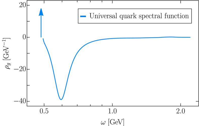
Figure 4: Universal quark spectral function as defined in 71 for light quark flavors in an isospin symmetric approximation from the spectral DSE results of [49]. The pole position is $m_{\text{sing}}\approx$485\text{\,}\mathrm{MeV}$$. The continuous tail contributes negatively to the mass function of the quark, resulting in a constituent quark mass of $M_{l}\approx$400\text{\,}\mathrm{MeV}$$.

The respective spectral function is depicted in Figure 4. Notably, the pole mass is larger than its corresponding constituent quark mass $M_{l}^{\text{DSE}}\approx$400\text{\,}\mathrm{MeV}$$, in contrast to the result in 69. The hierarchy of the masses found in [49] agrees with that obtained via vertex models widely used in bound state calculations with BSE-DSE systems: the real part of the leading complex singularity in the quark propagator is typically found to be considerably larger than the respective constituent mass [3, 50]. In turn, the Euclidean data that underlie the reconstruction leading to 69 are obtained in a qualitatively better approximation than that used in the direct realtime computation in [49].

Together this hints at a strong truncation dependence of the relation between quark constituent and pole mass which asks for a refined analysis. Such an analysis is beyond the scope of the present work and we only briefly discuss the underlying dynamics. For the sake of simplicity we restrict ourselves to the scenario with a spectral representation 73 and only comment on minor modifications in the general case 70 including also cc poles. With 67, 71a and 72, the constituent quark mass $m_{\text{const}}=M_{q}(0)$ and $m_{\text{sing}}$ are related by

$$m_{\textrm{sing}}^{2}={\cal C}m^{2}_{\text{const}}\,,$$ (75)

with

$${\cal C}={R+m_{\textrm{sing}}^{2}\int_{m_{\textrm{sign}}}^{\infty}\frac{\mathrm{d}\lambda}{\pi}\frac{\tilde{\rho}_{g}(\lambda)}{\lambda}}\,.$$ (76)

If cc poles are present, 76 is changed by

$$R\to\left(\frac{R}{\omega_{\textrm{sing}}^{2}}+\frac{\bar{R}}{\bar{\omega}_{\textrm{sing}}^{2}}\right)\,m_{\textrm{sing}}^{2}\,.$$ (77)

Equation 75 admits both, solutions with $M_{l}>m_{\text{sing}}$ and $M_{l}<m_{\text{sing}}$. In comparison to the sum rule 73, the spectral integral over $\tilde{\rho}_{g}$ in 75 carries an additional factor $1/\lambda^{2}$. Hence, the contributions of larger spectral values are suppressed. This is more clearly seen if rewriting the denominator in 75 with help of the sum rule 73,

$${\cal C}=1+\int_{m_{\textrm{sign}}}^{\infty}\frac{\mathrm{d}\lambda}{\pi}\,\lambda\,\tilde{\rho}_{g}(\lambda)\left[\frac{m_{\textrm{sing}}^{2}}{\lambda^{2}}-1\right]\,.$$ (78)

The integrand in 78 is counting the spectral weight of the scattering tail $\tilde{\rho}_{g}$, where the expression in the square bracket is an additional negative weight factor. For 70, the relation 78 has to be augmented with further but subleading terms proportional to $\textrm{Im}[\omega_{\textrm{sing}}^{2}]/m_{\textrm{sing}}^{2}$.

Equation 78 allows for a qualitative analysis of the required dynamics for the two cases. A simple scenario is provided by the spectral function computed in [49] and depicted in Figure 4. There, the weight of the scattering tail is concentrated at spectral values larger but close to the onset of the tail at $\lambda=m_{\textrm{sing}}$. Just above the onset, we have $\tilde{\rho}_{g}(\lambda\gtrsim m_{\textrm{sing}})\leq 0$ and hence the integral in 78 is positive, leading to ${\cal C}\approx 1.21$ and hence $M_{l}<m_{\text{sing}}$.

In turn, ${\cal C}<1$ is achieved for a scenario where the spectral function $\rho_{g}$ and hence also $\tilde{\rho}_{g}$ resembles more that of a physical particle. For the latter case the scattering tail $\tilde{\rho}_{g}>0$ and naturally we have ${\cal C}<1$ with $M_{l}>m_{\text{sing}}$. Translated to the present case with the quark spectral function, ${\cal C}<1$ is achieved for $\tilde{\rho}_{g}$ with a less pronounced or absent negative peak and more positive weight for larger spectral values. Such a scenario requires more genuine scatterings at large spectral values. The definite answer of whether or not these scatterings take place can only be answered in quantitatively reliable approximations that allow for momentum transfers in the vertices. In particular, within the truncation with constant vertex dressings used in [49] this specific question cannot be answered. In turn, while the truncation scheme used in [13, 29] is state-of-the-art, these computations are done in the Euclidean domain and the order of the constituent quark mass $M_{l}$ and $m_{\text{sing}}$ is obtained within a reconstruction of the pole position in the complex plane. Still, we consider the latter order as a strong hint for $m_{\text{sing}}<M_{l}$, but leave the decisive analysis to future work.

References

- Bertsch and Siemens [1983] G. Bertsch and P. j. Siemens, NUCLEAR FRAGMENTATION, Phys. Lett. B 126, 9 (1983).
- Chomaz [2002] P. Chomaz, The nuclear liquid gas phase transition and phase coexistence, AIP Conf. Proc. 610, 167 (2002), arXiv:nucl-ex/0410024 .
- Eichmann et al. [2016] G. Eichmann, H. Sanchis-Alepuz, R. Williams, R. Alkofer, and C. S. Fischer, Baryons as relativistic three-quark bound states, Prog. Part. Nucl. Phys. 91, 1 (2016), arXiv:1606.09602 [hep-ph] .
- Brambilla et al. [2014] N. Brambilla et al., QCD and Strongly Coupled Gauge Theories: Challenges and Perspectives, Eur. Phys. J. C 74, 2981 (2014), arXiv:1404.3723 [hep-ph] .
- de Forcrand and Fromm [2010] P. de Forcrand and M. Fromm, Nuclear Physics from lattice QCD at strong coupling, Phys. Rev. Lett. 104, 112005 (2010), arXiv:0907.1915 [hep-lat] .
- Kim et al. [2023] J. Kim, P. Pattanaik, and W. Unger, Nuclear liquid-gas transition in the strong coupling regime of lattice QCD, Phys. Rev. D 107, 094514 (2023), arXiv:2303.01467 [hep-lat] .
- Holt et al. [2013] J. W. Holt, N. Kaiser, and W. Weise, Nuclear chiral dynamics and thermodynamics, Prog. Part. Nucl. Phys. 73, 35 (2013), arXiv:1304.6350 [nucl-th] .
- Drischler et al. [2019] C. Drischler, K. Hebeler, and A. Schwenk, Chiral interactions up to next-to-next-to-next-to-leading order and nuclear saturation, Phys. Rev. Lett. 122, 042501 (2019), arXiv:1710.08220 [nucl-th] .
- Drischler et al. [2021] C. Drischler, S. Han, J. M. Lattimer, M. Prakash, S. Reddy, and T. Zhao, Limiting masses and radii of neutron stars and their implications, Phys. Rev. C 103, 045808 (2021), arXiv:2009.06441 [nucl-th] .
- Leonhardt et al. [2020] M. Leonhardt, M. Pospiech, B. Schallmo, J. Braun, C. Drischler, K. Hebeler, and A. Schwenk, Symmetric nuclear matter from the strong interaction, Phys. Rev. Lett. 125, 142502 (2020), arXiv:1907.05814 [nucl-th] .
- Mitter et al. [2015] M. Mitter, J. M. Pawlowski, and N. Strodthoff, Chiral symmetry breaking in continuum QCD, Phys. Rev. D91, 054035 (2015), arXiv:1411.7978 [hep-ph] .
- Rennecke [2015] F. Rennecke, Vacuum structure of vector mesons in QCD, Phys. Rev. D92, 076012 (2015), arXiv:1504.03585 [hep-ph] .
- Cyrol et al. [2018a] A. K. Cyrol, M. Mitter, J. M. Pawlowski, and N. Strodthoff, Nonperturbative quark, gluon, and meson correlators of unquenched QCD, Phys. Rev. D97, 054006 (2018a), arXiv:1706.06326 [hep-ph] .
- Braun et al. [2016] J. Braun, L. Fister, J. M. Pawlowski, and F. Rennecke, From Quarks and Gluons to Hadrons: Chiral Symmetry Breaking in Dynamical QCD, Phys. Rev. D94, 034016 (2016), arXiv:1412.1045 [hep-ph] .
- Fu et al. [2020] W.-j. Fu, J. M. Pawlowski, and F. Rennecke, QCD phase structure at finite temperature and density, Phys. Rev. D 101, 054032 (2020), arXiv:1909.02991 [hep-ph] .
- Fukushima et al. [2022] K. Fukushima, J. M. Pawlowski, and N. Strodthoff, Emergent hadrons and diquarks, Annals Phys. 446, 169106 (2022), arXiv:2103.01129 [hep-ph] .
- Serot and Walecka [1997] B. D. Serot and J. D. Walecka, Recent progress in quantum hadrodynamics, Int. J. Mod. Phys. E 6, 515 (1997), arXiv:nucl-th/9701058 .
- Shen et al. [2019] S. Shen, H. Liang, W. H. Long, J. Meng, and P. Ring, Towards an covariant density functional theory for nuclear structure, Prog. Part. Nucl. Phys. 109, 103713 (2019), arXiv:1904.04977 [nucl-th] .
- Gies and Wetterich [2004] H. Gies and C. Wetterich, Universality of spontaneous chiral symmetry breaking in gauge theories, Phys. Rev. D69, 025001 (2004), arXiv:hep-th/0209183 [hep-th] .
- Braun [2009] J. Braun, The QCD Phase Boundary from Quark-Gluon Dynamics, Eur. Phys. J. C 64, 459 (2009), arXiv:0810.1727 [hep-ph] .
- Dupuis et al. [2021] N. Dupuis, L. Canet, A. Eichhorn, W. Metzner, J. M. Pawlowski, M. Tissier, and N. Wschebor, The nonperturbative functional renormalization group and its applications, Phys. Rept. 910, 1 (2021), arXiv:2006.04853 [cond-mat.stat-mech] .
- Fu [2022] W.-j. Fu, QCD at finite temperature and density within the fRG approach: an overview, Commun. Theor. Phys. 74, 097304 (2022), arXiv:2205.00468 [hep-ph] .
- Jung et al. [2017] C. Jung, F. Rennecke, R.-A. Tripolt, L. von Smekal, and J. Wambach, In-Medium Spectral Functions of Vector- and Axial-Vector Mesons from the Functional Renormalization Group, Phys. Rev. D 95, 036020 (2017), arXiv:1610.08754 [hep-ph] .
- Jung and von Smekal [2019] C. Jung and L. von Smekal, Fluctuating vector mesons in analytically continued functional RG flow equations, Phys. Rev. D 100, 116009 (2019), arXiv:1909.13712 [hep-ph] .
- Cohen [2003] T. D. . Cohen, Functional integrals for QCD at nonzero chemical potential and zero density, Phys. Rev. Lett. 91, 222001 (2003), arXiv:hep-ph/0307089 [hep-ph] .
- van Dalen et al. [2005] E. N. E. van Dalen, C. Fuchs, and A. Faessler, Effective nucleon masses in symmetric and asymmetric nuclear matter, Phys. Rev. Lett. 95, 022302 (2005), arXiv:nucl-th/0502064 .
- Baldo et al. [2014] M. Baldo, G. F. Burgio, H. J. Schulze, and G. Taranto, Nucleon effective masses within the Brueckner-Hartree-Fock theory: Impact on stellar neutrino emission, Phys. Rev. C 89, 048801 (2014), arXiv:1404.7031 [nucl-th] .
- Shang et al. [2020] X. L. Shang, A. Li, Z. Q. Miao, G. F. Burgio, and H. J. Schulze, Nucleon effective mass in hot dense matter, Phys. Rev. C 101, 065801 (2020), arXiv:2001.03859 [nucl-th] .
- Gao et al. [2021] F. Gao, J. Papavassiliou, and J. M. Pawlowski, Fully coupled functional equations for the quark sector of QCD, Phys. Rev. D 103, 094013 (2021), arXiv:2102.13053 [hep-ph] .
- Haas et al. [2014] M. Haas, L. Fister, and J. M. Pawlowski, Gluon spectral functions and transport coefficients in Yang–Mills theory, Phys. Rev. D90, 091501 (2014), arXiv:1308.4960 [hep-ph] .
- Ilgenfritz et al. [2018] E.-M. Ilgenfritz, J. M. Pawlowski, A. Rothkopf, and A. Trunin, Finite temperature gluon spectral functions from lattice QCD, Eur. Phys. J. C78, 127 (2018), arXiv:1701.08610 [hep-lat] .
- Cyrol et al. [2018b] A. K. Cyrol, J. M. Pawlowski, A. Rothkopf, and N. Wink, Reconstructing the gluon, SciPost Phys. 5, 065 (2018b), arXiv:1804.00945 [hep-ph] .
- Dudal et al. [2019] D. Dudal, O. Oliveira, M. Roelfs, and P. Silva, Spectral representation of lattice gluon and ghost propagators at zero temperature, (2019), arXiv:1901.05348 [hep-lat] .
- Li et al. [2019] S. W. Li, P. Lowdon, O. Oliveira, and P. J. Silva, The generalised infrared structure of the gluon propagator, (2019), arXiv:1907.10073 [hep-th] .
- Hayashi and Kondo [2021] Y. Hayashi and K.-I. Kondo, Reconstructing confined particles with complex singularities, Phys. Rev. D 103, L111504 (2021), arXiv:2103.14322 [hep-th] .
- Horak et al. [2022a] J. Horak, J. M. Pawlowski, J. Rodríguez-Quintero, J. Turnwald, J. M. Urban, N. Wink, and S. Zafeiropoulos, Reconstructing QCD spectral functions with Gaussian processes, Phys. Rev. D 105, 036014 (2022a), arXiv:2107.13464 [hep-ph] .
- Horak et al. [2023] J. Horak, J. M. Pawlowski, J. Turnwald, J. M. Urban, N. Wink, and S. Zafeiropoulos, Nonperturbative strong coupling at timelike momenta, Phys. Rev. D 107, 076019 (2023), arXiv:2301.07785 [hep-ph] .
- Karsch and Kitazawa [2009] F. Karsch and M. Kitazawa, Quark propagator at finite temperature and finite momentum in quenched lattice QCD, Phys. Rev. D 80, 056001 (2009), arXiv:0906.3941 [hep-lat] .
- Mueller et al. [2010] J. A. Mueller, C. S. Fischer, and D. Nickel, Quark spectral properties above Tc from Dyson-Schwinger equations, Eur. Phys. J. C 70, 1037 (2010), arXiv:1009.3762 [hep-ph] .
- Qin and Rischke [2013] S.-x. Qin and D. H. Rischke, Quark Spectral Function and Deconfinement at Nonzero Temperature, Phys. Rev. D 88, 056007 (2013), arXiv:1304.6547 [nucl-th] .
- Fischer et al. [2018] C. S. Fischer, J. M. Pawlowski, A. Rothkopf, and C. A. Welzbacher, Bayesian analysis of quark spectral properties from the Dyson-Schwinger equation, Phys. Rev. D 98, 014009 (2018), arXiv:1705.03207 [hep-ph] .
- Kamikado et al. [2014] K. Kamikado, N. Strodthoff, L. von Smekal, and J. Wambach, Real-time correlation functions in the model from the functional renormalization group, Eur. Phys. J. C74, 2806 (2014), arXiv:1302.6199 [hep-ph] .
- Fischer and Huber [2020] C. S. Fischer and M. Q. Huber, Landau gauge Yang-Mills propagators in the complex momentum plane, Phys. Rev. D 102, 094005 (2020), arXiv:2007.11505 [hep-ph] .
- Pawlowski and Strodthoff [2015] J. M. Pawlowski and N. Strodthoff, Real time correlation functions and the functional renormalization group, Phys. Rev. D92, 094009 (2015), arXiv:1508.01160 [hep-ph] .
- Pawlowski et al. [2018] J. M. Pawlowski, N. Strodthoff, and N. Wink, Finite temperature spectral functions in the O(N)-model, Phys. Rev. D98, 074008 (2018), arXiv:1711.07444 [hep-th] .
- Horak et al. [2020] J. Horak, J. M. Pawlowski, and N. Wink, Spectral functions in the -theory from the spectral DSE, Phys. Rev. D 102, 125016 (2020), arXiv:2006.09778 [hep-th] .
- Horak et al. [2021] J. Horak, J. Papavassiliou, J. M. Pawlowski, and N. Wink, Ghost spectral function from the spectral Dyson-Schwinger equation, Phys. Rev. D 104, 10.1103/PhysRevD.104.074017 (2021), arXiv:2103.16175 [hep-th] .
- Horak et al. [2022b] J. Horak, J. M. Pawlowski, and N. Wink, On the complex structure of Yang-Mills theory, (2022b), arXiv:2202.09333 [hep-th] .
- Horak et al. [2022c] J. Horak, J. M. Pawlowski, and N. Wink, On the quark spectral function in QCD, (2022c), arXiv:2210.07597 [hep-ph] .
- Windisch [2017] A. Windisch, Analytic properties of the quark propagator from an effective infrared interaction model, Phys. Rev. C 95, 045204 (2017), arXiv:1612.06002 [hep-ph] .