Shape of my heart: Cardiac models through learned signed distance functions

Abstract

The efficient construction of an anatomical model is one of the major challenges of patient-specific in-silico models of the human heart. Current methods frequently rely on linear statistical models, allowing no advanced topological changes, or requiring medical image segmentation followed by a meshing pipeline, which strongly depends on image resolution, quality, and modality. These approaches are therefore limited in their transferability to other imaging domains. In this work, the cardiac shape is reconstructed by means of three-dimensional deep signed distance functions with Lipschitz regularity. For this purpose, the shapes of cardiac MRI reconstructions are learned from public databases to model the spatial relation of multiple chambers in Cartesian space. We demonstrate that this approach is also capable of reconstructing anatomical models from partial data, such as point clouds from a single ventricle, or modalities different from the trained MRI, such as electroanatomical mapping, and in addition, allows us to generate new anatomical shapes by randomly sampling latent vectors.

1 Introduction

Modern personalized precision medicine frequently targets patient-specific therapies with improved therapy outcomes, reduced intervention times, and thus lower costs. In the case of cardiac personalized treatment, this necessitates complex simulation models from patient data [1]. This future vision of personalized cardiac treatment heavily relies on generated 3D models, which should represent the anatomy of the corresponding patient.

Current methods to generate anatomical models usually require CT or MR images, which are segmented and subsequently meshed [2]. Yet, while automatic cardiac image segmentation is well-researched and constantly improving thanks to machine learning [3, 4, 5], it is limited to a specific image modality and resolution. Other modalities such as electroanatomical catheter mapping [6] are difficult to fit within standard frameworks, albeit they are very important for patient-specific modelling [7].

In this work, we propose the use of implicitly learned representations through signed distance functions (SDFs). We start from the DeepSDF method [8], which encodes SDF-based surfaces through a decoder-only neural network with a small-dimensional input latent code. As a matter of fact, the neural network is a cardiac shape atlas. Shape inference can be achieved from location measurements such as electro-anatomical mappings and is applicable to arbitrary resolutions. Additionally, interpolation in the latent space yields shape interpolation in the physical space, a useful feat to create novel shapes. Differently from the original DeepSDF method, here we take advantage of Lipschitz-regularized neural networks [9] so to avoid overfitting of the network and to enforce smooth interpolations between samples in the latent space. This method is especially efficient for learning on relatively small training sets as considered here.

We demonstrate that this Lipschitz-regularized DeepSDF architecture is suited for constructing cardiac models by learning from a database of $44$ publicly available, post-processed cardiac models. The resulting DeepSDF model is designed to encode bi-ventricular shapes and also infer new shapes from sparse point clouds, even if only partial domains are available (e.g., only endocardial measurements of a single chamber such as is often the case in electroanatomical mapping). In summary, our work will provide the following contributions to the field of anatomical cardiac modeling:

1. applying the DeepSDF methodology to the cardiac domain on the example of bi-ventricular models,

2. demonstrating superior robustness to noise in comparison to many state-of-the-art methods,

3. showing that interpolation and (limited) extrapolation of biventricular models in the latent space can generate meaningful novel bi-ventricular shapes,

4. reconstructing a bi-ventricular shape from in-vivo measurements of an electroanatomical mapping procedure.

2 Related Work

Here, we present an overview of shape reconstruction methods for both general shapes and cardiac-specific applications.

2.1 Methods for Shape Reconstruction

Surface reconstruction from point clouds is an intensively-researched topic and provides a variety of possible approaches [10]. Classical approaches assume no prior knowledge of the given point clouds, but in turn, require dense point clouds and are often sensitive to noise [11, 12, 13, 14, 15]. Modern deep-learning approaches try to overcome these limitations by learning prior information about shapes through a database of given meshes/shapes. In many cases, these methods rely on learned SDFs [8], occupancy fields [16], level sets [17] or implicit fields [18] which are subsequently discretized and meshed. Point2Mesh [19] uses an input point cloud to generate a shape prior, which is then used to reconstruct a mesh by shrinking an initial mesh to the point cloud.

In this context, the DeepSDF method is one of the most active fields of research. Such methods usually try to infer a multitude of shapes from at least partially dense point clouds in the presence of noise. However, this method is prone to overfitting the data, thus often requiring regularization both in the latent space, as well as in the neural network by imposing dropout rules [8]. In [9], Lipschitz-regularized linear layers are proposed, which are able to overcome some of these limitations and improve interpolation and extrapolation in latent space. Alternative forms of regularization are, for instance, based on the eikonal equation [20]. Other methods rely on local SDFs [21, 22, 23, 24], neural-pulls [25], or learned unsigned distance functions [26]. For further methods and comparisons, we refer the reader to [10].

Statistical Shape Models (SSMs) are classical methods for (cardiac) shape reconstruction, which are tailored to the whole heart [27, 28, 29, 30, 31, 32], the atria [33], or the ventricles [34, 35]. Only a few works have shown that these deep learning methods can be applied to the cardiac domain to reconstruct cardiac shapes from sparse point clouds or annotated imaging slices [36, 37]. Such methods also use a shape database that is usually restricted to the same shape across different patients to better reconstruct the shape of new patients. In [38], the authors use variational mesh autoencoders to reconstruct cardiac shapes from raw cine MRI images. Kong et al. [39] use a graph convolutional network to reconstruct cardiac shapes from CT and MT image data. In [40], the authors exploit convolutional neural networks to reconstruct left atrial shapes from point clouds. However, to the best of our knowledge, there is no method to directly infer bi-ventricular endo- and epicardial shapes using DeepSDF.

3 Method

In this section, we comment on the representation of cardiac shapes by learned SDFs and provide details about training and shape completion.

3.1 General Setting

We assume that each shape describing the heart is volumetrically represented as an SDF given by $f_{S}:\mathbb{R}^{3}\rightarrow\mathbb{R}$ mapping from spatial points $\mathbf{x}\in\mathbb{R}^{3}$ to their respective signed distances $s\in\mathbb{R}$. These signed distances encode the signed projection distance at a point $\mathbf{x}$ to the surface (negative values inside, positive values outside). In such a way, the cardiac surface is represented as the zero-level set of this SDF, i.e., $f_{S}^{-1}(0)$. A straightforward approach to learning such an SDF for arbitrary shapes involves representing the SDF by a neural network $S_{\theta}:\mathbb{R}^{3}\rightarrow\mathbb{R}$, in which case the SDF is fully defined by the network’s architecture and weights $\theta$. However, modeling surfaces solely through their neural network weights would necessitate a separate SDF and subsequent neural network for each individual surface, while also neglecting any similarities between the available training shapes. Following [8], we instead model all shapes using a single neural network and additionally provide this network with a $d$-dimensional latent representation $\mathbf{z}\in\mathbb{R}^{d}$ of the shape as an additional input, together with the aforementioned spatial coordinates, i.e. $S_{\theta}:\mathbb{R}^{3+d}\rightarrow\mathbb{R}$. Hence, we encode multiple shapes with the same network, but different latent codes.

In this paper, we want to apply this method to the case of bi-ventricular anatomical data. Bi-ventricular surfaces have limited curvature and fewer details than traditional computer graphics models but are in general challenging since they consist of left and right endocardial and epicardial surfaces ($4$ in total) that are closely connected. We propose to model each of these surfaces with a shared latent code and neural network by letting the DeepSDF simultaneously estimate a signed distance for each of the bi-ventricular surfaces $\mathbf{s}=(s_{1},s_{2},s_{3},s_{4})^{\top}\in\mathbb{R}^{4}$. In summary, the learned DeepSDF is given by the vector-valued function $\mathbf{S}_{\theta}:\mathbb{R}^{3+d}\rightarrow\mathbb{R}^{4}$.

3.2 Training and Network Architecture

The anatomical samples $X_{i}\coloneqq\left(\mathbf{x}_{k},\mathbf{s}_{k}\right)_{k=1}^{K_{i}}$ used for learning are $K_{i}$ pairs of spatial coordinates $\mathbf{x}_{k}$ with their sampled signed distance vector $\mathbf{s}_{k}$ for the $i$-th biventricular shape. The set of all $N$ available anatomical bi-ventricular samples is denoted as $X\coloneqq\left(X_{i}\right)_{i=1}^{N}$. To each anatomical shape $i$, we associate a coupled latent code representation $\mathbf{z}_{i}\in\mathbb{R}^{d}$ also learned from data. We denote the set of learned latent codes as $Z\coloneqq\left(\mathbf{z}_{i}\right)_{i=1}^{N}$. Our goal during training is to minimize the mismatch between the sampled signed distances and the ones estimated by the network through a simple quadratic loss term. Additionally, to restrict the latent codes $Z$, we follow [8] and assume a zero mean Gaussian prior distribution with covariance $\sigma^{2}I$ on the latent codes, which gives rise to the complete loss term

$$\mathcal{L}(\theta,Z)=\frac{1}{N}\sum_{i=1}^{N}\sum_{(\mathbf{x}_{k},\mathbf{s}_{k})\in X_{i}}\frac{1}{4K_{i}}\lVert\mathbf{S}_{\theta}(\mathbf{x}_{k},\mathbf{z}_{i})-\mathbf{s}_{k}\rVert^{2}+\frac{1}{\sigma^{2}}\|\mathbf{z}_{i}\|^{2}_{2}.$$

The parameter $\sigma$ is used to balance between reconstruction accuracy for the training shapes and regularity in the latent space, which is essential for shape completion as described in Section 3.3. See Section 4.2 for the choice of $\sigma$ in our model.

In [9], it was shown that learning $\mathcal{L}$ directly may result in overfitting and might provide poor interpolation properties for the latent space. To overcome these issues, a Lipschitz penalization on the network was proposed in order to better control the smoothness. For this purpose, the Lipschitz bound $L$ of the network is estimated by $L=\prod_{i=1}^{M}\|W_{i}\|_{p}$ for an $M$-layer deep network, where $W_{i}$ are the network weights of the $i$-th layer. We closely follow the implementation of [9] where the linear layers of our network are replaced with Lipschitz-normalized layers. For each layer an additional weight $c_{i}$ is introduced such that $\text{softplus}(c_{i})=\ln(1+e^{c_{i}})$ serves as an upper bound $\text{softplus}(c_{i})\geq\|W_{i}\|_{p}$ for the Lipschitz constant. The softplus function numerically prevents the occurrence of negative Lipschitz constraints during the optimization but since the $c_{i}$ are usually large constants one has $\text{softplus}(c_{i})\approx c_{i}$. Note that the norm $p=\infty$ is chosen out of computational convenience. Integrating this Lipschitz-regularization into our previous loss-functional $\mathcal{L}$ leads to our finally used cost-functional

$$J(\theta,Z,C)=\mathcal{L}(\theta,Z)+\alpha\prod_{c_{i}\in C}\text{softplus}(c_{i}),$$ (1)

where $C=(c_{i})_{i=1}^{M}$ denotes per-layer Lipschitz constants as optimization variables.

Figure 1: A schematic representation of the employed DeepSDF.

As mentioned, for samples $X_{i}\coloneqq\left(\mathbf{x}_{k},\mathbf{s}_{k}\right)_{k=1}^{K_{i}}$ the network inputs are the latent code $\mathbf{z}_{i}$ and the spatial coordinates $\mathbf{x}_{i}$ of the sample point. Following [9] the spatial coordinates are multiplied by the factor $C_{s}=100$ to balance the Lipschitz regularity of the latent space and the spatial coordinates. We use $5$ hidden layers with $256$ neurons and $\tanh$ activation functions. In the third hidden layer, the latent code and the spatial coordinate are concatenated to the output of the previous layer. The last layer is a linear layer with four signed distance functions as output, one for each of the left, right, epi- and endocardial surfaces. The latent code size was chosen as $d=64$. A schematic representation of the network is shown in Figure 1.

3.3 Shape Completion

After learning the SDF network, a new anatomical bi-ventricular shape can be inferred from sparse point clouds of any combination of surfaces or given signed distance. For this, we consider $K$ given samples consisting of triplets $\tilde{Y}$ of spatial coordinates $\mathbf{x}_{k}\in\mathbb{R}^{3}$, a single signed distance $s_{k}\in\mathbb{R}$, and an index of the surface $j_{k}\in\{1,2,3,4\}$. If a point $\mathbf{x}_{k}$ lies on the surface $j_{k}$, then $s_{k}=0$. Finding the bi-ventricular reconstruction of a point cloud thus reduces to finding its latent code representation $\mathbf{z}$ by minimizing the following problem

$$\min_{\mathbf{z}}\frac{1}{K}\sum_{(\mathbf{x}_{k},s_{k},j_{k})\in\tilde{Y}}\left(\left(\mathbf{S}_{\theta}(\mathbf{x}_{k},\mathbf{z})\right)_{j_{k}}-s_{k}\right)^{2}+\frac{\beta}{\sigma^{2}}\|\mathbf{z}\|_{2}^{2},$$ (2)

where the subscript refers to the vector component and $\beta$ is an additional weight that is increased depending on the noise of the input point cloud. For noise-free point clouds, we set $\beta=1$ to obtain the maximum-a-posterior (MAP) estimation [8].

For noisy input point clouds, the expected data loss of a perfect reconstruction can be approximated with the variance of the noise $\xi$. We set $\beta=C_{b}\xi$, where $C_{b}=100$ is a chosen blow-up factor. In the case of real-world data, the underlying noise structure is unknown and estimated as follows: We start with a reconstruction $\mathbf{S}_{\theta}^{0}$ for an arbitrary initial noise estimation $\bar{\xi}_{0}$. We then iteratively estimate the empirical variance $\bar{\xi}_{n+1}^{2}$ based on $\mathbf{S}_{\theta}^{n}$ via

$$\bar{\xi}_{n+1}^{2}=\frac{1}{K-1}\sum_{(\mathbf{x}_{k},s_{k},j_{k})\in\tilde{Y}}\left(\left(\mathbf{S}_{\theta}^{n}(\mathbf{x}_{k},\mathbf{z})\right)_{j_{k}}-s_{k}\right)^{2}.$$ (3)

This estimation exhibits a high experimental convergence rate (see Section 4.5).

4 Experiments

In this section, we state details of the dataset preparation, training procedure and the network architecture. Moreover, we introduce distinct metrics for the evaluation of the surface reconstruction quality, which are exploited in all benchmarks. Finally, we evaluate the network on in-vivo measured catheter data.

4.1 Dataset

Based on [41, 42], we built a shape library of watertight 3D shapes for endo-/epicardium of the left/right ventricles ($4$ shapes in total). The generated shape data will be published upon acceptance.

Surface mesh generation

As a basis for our meshes, we used the publicly available data described in [41, 42]. Our dataset was produced by applying the following procedure to each of the meshes: First, after loading the data, we localize the left ventricular apex using the available universal ventricular coordinates (UVCs, [43]) and use it as the Cartesian origin for each of the meshes. Next, we extract the left/right ventricular (LV/RV) endo-/epicardia by using the available surface tags. The provided meshes encode the walls and valves into separate tags, from which we extracted the surfaces. We then identify all points of the wall that touch the associated valve (e.g. LV wall with mitral and aortic valves). To identify all reachable points, we compute an eikonal solution using [44] by placing an initial point on the inside of the wall (closest to the blood pool) with minimal velocity across points that touch any of the valves. The wall is then separated into epi- and endocardium by applying a thresholding filter on the solution. Finally, we remove non-manifold parts, recalculate the inside/outside orientation and close the surface to receive a watertight, proper manifold surface for the endo- and epicardia separately. Note that all steps exploit VTK [45] through PyVista [46].

Surface sampling

The training data was then generated by sampling $3000$ surface points (surface samples) and additional $1000$ points, displaced in normal direction randomly (uniform) by up to $30$mm (band samples). Two point clouds were sampled with a curvature-based weighting to create more samples around features of interest (e.g. apex, valves). Specifically, we generated the dataset samples using face-weights $w$ following [47, Eq. 2.6] that are defined as follows: consider a 2-dimensional compact surface $M$, isometrically embedded in $\mathbb{R}^{3}$, with its Gaussian curvature $\kappa$ and mean curvature $\eta$. The weighting function is then defined as

$$w_{\lambda,\rho}(\mathbf{x})=\frac{\lambda|\kappa(\mathbf{x})|^{\rho}}{\int_{M}|\kappa(\xi)|^{\rho}\operatorname{d}\!{\text{vol}_{M}}(\xi)}+\frac{(1-\lambda)|\eta(\mathbf{x})|^{\rho}}{\int_{M}|\eta(\xi)|^{\rho}\operatorname{d}\!{\text{vol}_{M}}(\xi)}.$$ (4)

In our experiments, we used $w_{0.1,0.75}$ as the curvature weight, purely by visual inspection. We used the library trimesh [48] for sampling and computing $\kappa$ and $\eta$.

4.2 Numerical experiments

In this section, we present the numerical results obtained with the proposed method. The dataset is split into a training set (36), a validation set (4), and a test set (4). During the training process, we optimize both the network parameters $\theta$ and the latent code representations $\mathbf{z}_{i}$ of the training data. The network is fit to $4$ surfaces, namely the epi- and endocardium of the right and left ventricle, and the associated hyperparameters $\sigma$ and $\alpha$ are optimized for the best performance of the reconstruction of the validation set in the shape completion process. For the loss term, we thus obtained $1/\sigma^{2}\approx 1.8\times 10^{-7}$ and $\alpha=1.9\times 10^{-6}$. The network is trained with the Adam optimizer [49] for $3000$ epochs with a learning rate of $0.005$ which is decreased twice with the factor of 0.2 after $2700$ and $2900$ epochs. For the mesh generation, we compute the signed distance function on a $128^{3}$ grid on the bounding box of all training points. The reconstruction quality of the training models at the end of training is depicted in Figure 2.

Figure 2: Comparison of ground truth meshes with reconstruction on the training dataset. The reconstructed meshes are color-coded with the signed distance to the ground truth mesh in mm.

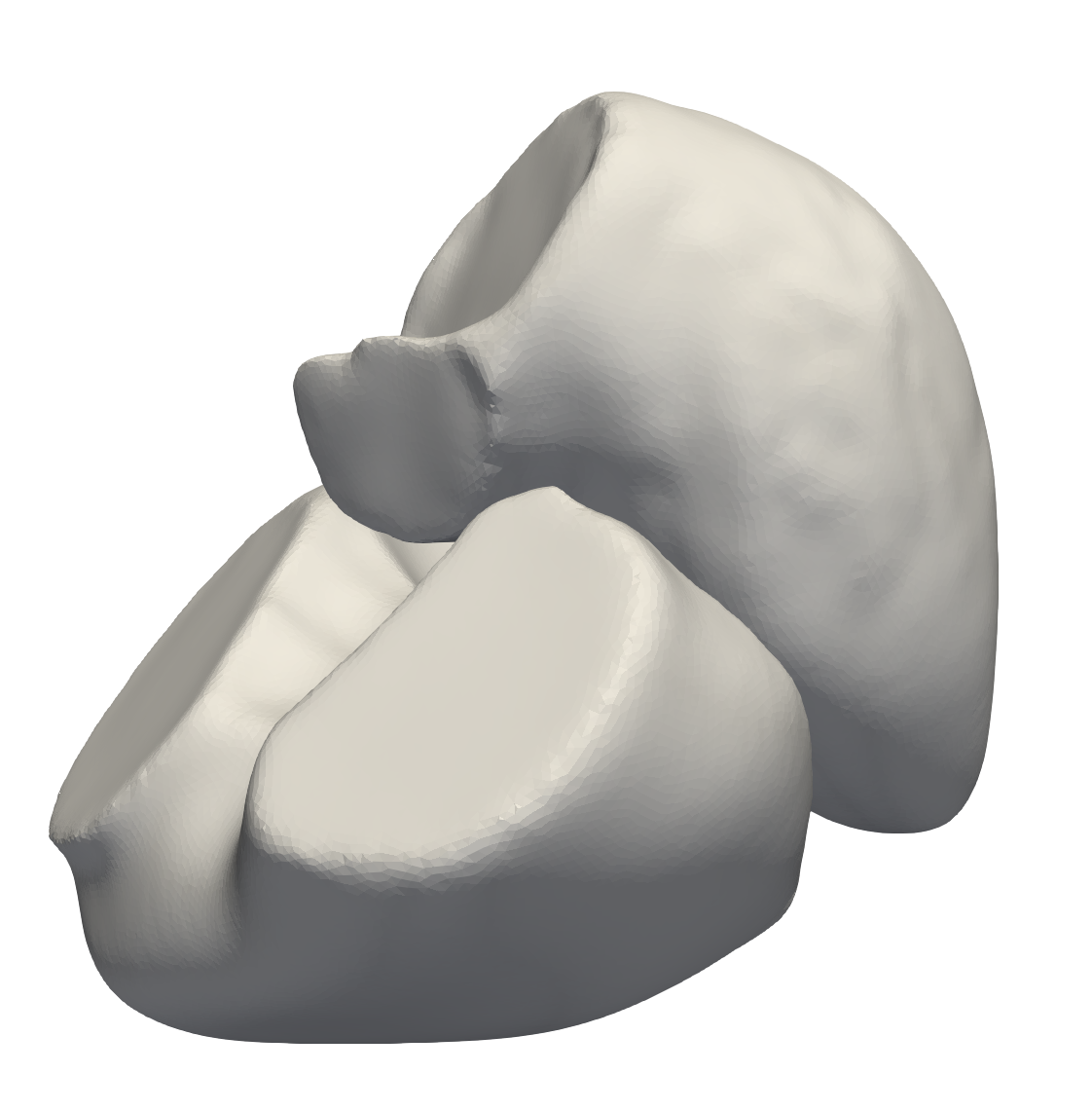
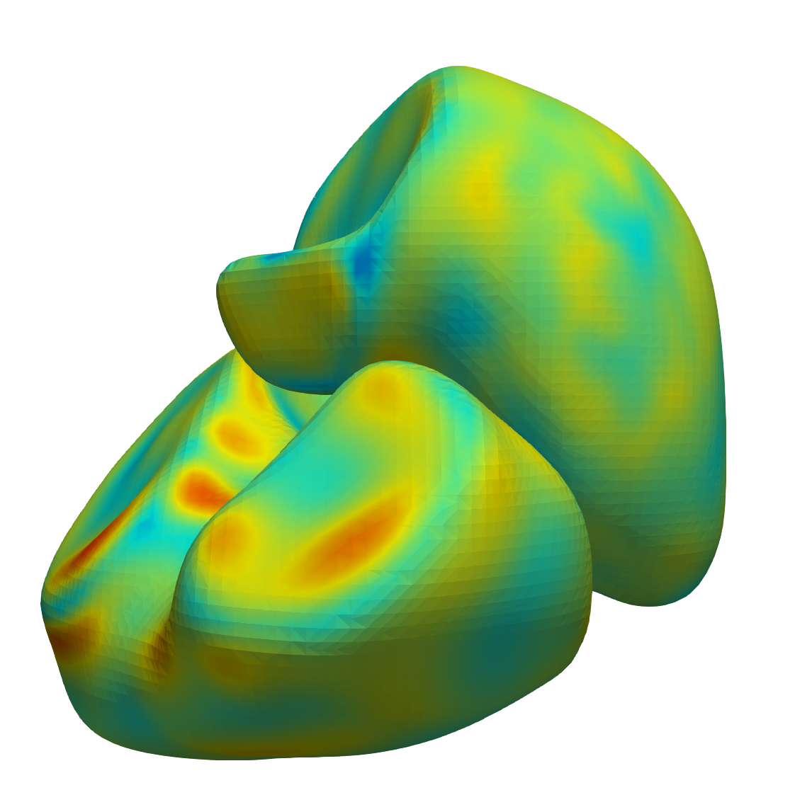
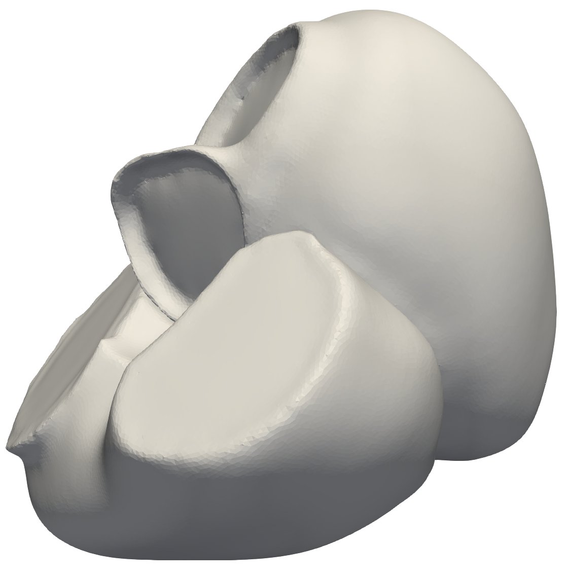
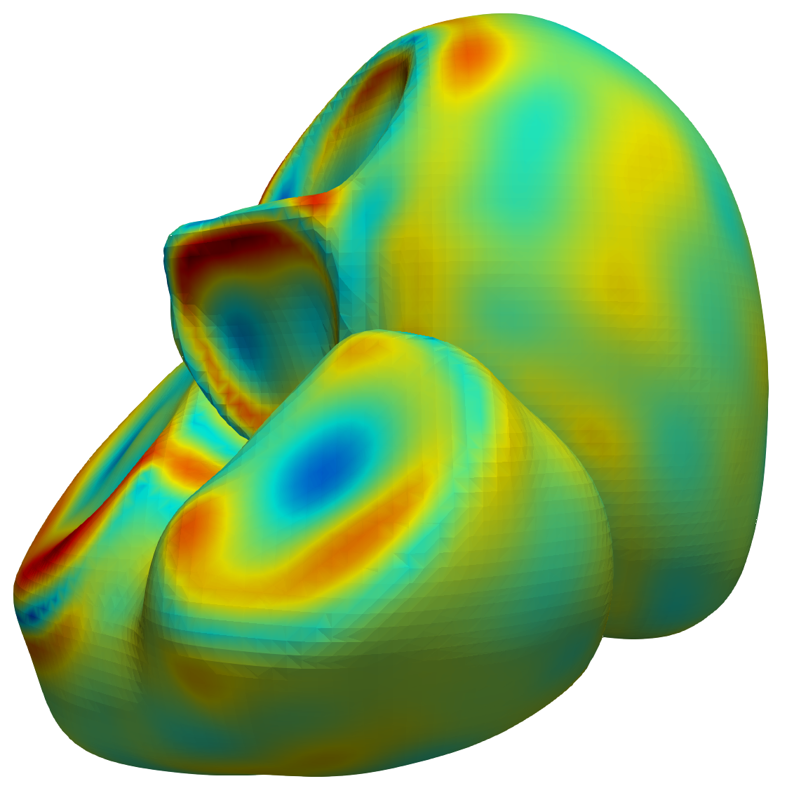
We test the regularity of our network with respect to the latent space input with inter- and extrapolation between two latent space representations of the training dataset. The shapes of the reconstructed hearts change uniformly between every inter- and extrapolation point and generate meaningful results (see Figure 3).

Figure 3: The figure shows the generation of heart models via interpolation and extrapolation of latent code vectors. In detail, we take two latent code representations $\mathbf{z}_{1},\mathbf{z}_{2}$ from the training dataset and decode the linear combinations $t\mathbf{z}_{1}+(1-t)\mathbf{z}_{2}$. We present the reconstructed endocardium of the left and right ventricle.

With our model, we are able to learn multiple implicit surfaces at the same time and encode them in a joint latent space representation. Therefore, it is easily possible to calculate the latent code during inference time based on an arbitrary subset of surface points. We test this by sampling sparse point clouds on the endocardium of the left ventricles from the test set and optimizing the latent code according to Equation 2. Not only is our method capable of a close reconstruction of the endocardium of the left ventricle, but it can also predict the shape of the other three surfaces (Figure 4). Numerical results of the reconstruction quality on the endocardium of the left ventricle can be found in Section 4.4.

Figure 4: We reconstruct all four surfaces from 50 points on the endocardium of the left ventricle. The reconstructed meshes are color-coded with the mesh distance, i.e. the distance to the nearest point on the ground truth mesh in mm.

4.3 Metrics

To quantify the quality of reconstructed meshes we use the L2-Chamfer-distance (CD), the Hausdorff-distance (HD), and a Large deformation diffeomorphic metric mapping (LDDMM) loss terms between the reconstructed mesh and the ground truth mesh. We calculate the L2-Chamfer distance and the Hausdorff distance by sampling 50 000 points on each mesh. For two point clouds $\mathbf{X}$ and $\mathbf{Y}$ the CD is given as

$$d_{\text{CD}}(\mathbf{X},\mathbf{Y})=\frac{1}{|\mathbf{X}|}\sum_{x\in\mathbf{X}}\min_{y\in\mathbf{Y}}\|x-y\|_{2}+\frac{1}{|\mathbf{Y}|}\sum_{y\in\mathbf{Y}}\min_{x\in\mathbf{X}}\|x-y\|_{2}.$$

The Hausdorff distance (HD) is defined as

$$d_{\text{HD}}(\mathbf{X},\mathbf{Y})=\max\{\max_{x\in\mathbf{X}}\min_{y\in\mathbf{Y}}\|x-y\|_{2},\max_{y\in\mathbf{Y}}\min_{x\in\mathbf{X}}\|x-y\|_{2}\}.$$

With the LDDMM loss, we measure how well the reconstructed mesh $\mathcal{M}_{r}$ can be registered to the original ground truth mesh $\mathcal{M}_{gt}$. To obtain numerically comparable results across the different methods we first remesh the results to obtain meshes with the same resolution (for this task, we use the Blender software package [50] with a voxel resolution of 0.9 mm). To obtain the LDDMM loss, we calculate the center points $c_{F}$, the normals $n_{F}$ and the area $A_{F}$ of every face $F$ from the set of faces $\mathcal{F}_{r}$ and $\mathcal{F}_{gt}$, respectively. For $\gamma=1$ let

$$C(\mathcal{F}_{1},\mathcal{F}_{2})=\sum_{F_{1}\in\mathcal{F}_{1}}\sum_{F_{2}\in\mathcal{F}_{2}}e^{-\gamma\|c_{F_{1}}-c_{F_{2}}\|_{2}^{2}}\langle n_{F_{1}},n_{F_{2}}\rangle A_{F_{1}}A_{F_{2}}.$$

Then, the LDDMM loss is defined as

$$d_{L}(\mathcal{M}_{gt},\mathcal{M}_{r})=C(\mathcal{F}_{gt},\mathcal{F}_{gt})+C(\mathcal{F}_{r},\mathcal{F}_{r})-2C(\mathcal{F}_{gt},\mathcal{F}_{r}).$$

4.4 Validation

	$\xi$	$n$	Points2Surf	Point2Mesh	SSM	ours
Chamfer Distance	$0$	50	-	1.19$\pm$0.10	4.57$\pm$3.03	0.84$\pm$0.13
		200	-	0.59$\pm$0.10	3.36$\pm$1.59	0.55$\pm$0.08
		500	1.26$\pm$0.06	0.55$\pm$0.05	2.85$\pm$1.46	0.51$\pm$0.06
		2000	0.36$\pm$0.03	0.54$\pm$0.03	2.62$\pm$1.88	0.50$\pm$0.08
	$2$	50	-	1.55$\pm$0.07	4.61$\pm$2.91	1.34$\pm$0.26
		200	-	1.23$\pm$0.13	3.59$\pm$1.87	1.15$\pm$0.19
		500	1.45$\pm$0.06	0.91$\pm$0.08	2.91$\pm$1.50	1.04$\pm$0.16
		2000	0.77$\pm$0.04	0.76$\pm$0.06	2.61$\pm$1.82	1.16$\pm$0.33
	$5$	50	-	3.14$\pm$0.31	4.52$\pm$2.30	2.35$\pm$0.34
		200	-	3.41$\pm$0.71	4.06$\pm$2.47	2.19$\pm$0.26
		500	2.84$\pm$0.38	3.91$\pm$1.12	3.23$\pm$1.66	1.94$\pm$0.23
		2000	1.95$\pm$0.09	5.97$\pm$0.41	2.80$\pm$1.68	3.06$\pm$0.63
Hausdorff Distance	$0$	50	-	8.66$\pm$1.15	15.06$\pm$9.85	4.68$\pm$1.26
		200	-	3.67$\pm$0.84	13.37$\pm$9.06	3.09$\pm$1.17
		500	6.26$\pm$0.19	2.18$\pm$0.30	13.55$\pm$11.13	2.93$\pm$0.88
		2000	1.86$\pm$0.49	1.27$\pm$0.11	16.67$\pm$16.79	2.80$\pm$0.80
	$2$	50	-	7.77$\pm$1.86	16.37$\pm$10.18	5.94$\pm$1.16
		200	-	6.01$\pm$0.32	14.41$\pm$10.27	5.96$\pm$1.52
		500	9.58$\pm$1.75	4.23$\pm$0.79	13.68$\pm$11.23	5.53$\pm$0.64
		2000	8.40$\pm$0.86	5.48$\pm$2.46	17.44$\pm$17.13	6.55$\pm$2.51
	$5$	50	-	14.65$\pm$2.83	15.88$\pm$8.05	9.26$\pm$1.17
		200	-	13.22$\pm$1.56	15.83$\pm$11.58	8.14$\pm$0.46
		500	17.38$\pm$0.81	14.89$\pm$2.88	15.09$\pm$11.88	9.19$\pm$1.33
		2000	16.17$\pm$1.00	19.27$\pm$2.43	18.26$\pm$14.50	11.72$\pm$4.54
LDDMM Loss ($\times 10^{3}$)	$0$	50	-	47.82$\pm$8.63	83.89$\pm$18.78	35.20$\pm$7.88
		200	-	23.93$\pm$10.32	78.56$\pm$17.36	20.60$\pm$7.32
		500	55.36$\pm$10.82	20.47$\pm$6.01	74.79$\pm$17.87	17.71$\pm$5.71
		2000	5.44$\pm$2.05	18.62$\pm$4.74	70.628$\pm$20.00	17.30$\pm$7.70
	$2$	50	-	54.36$\pm$7.94	85.29$\pm$20.54	57.80$\pm$17.67
		200	-	57.29$\pm$11.35	80.64$\pm$16.93	52.71$\pm$12.36
		500	60.98$\pm$9.27	44.12$\pm$10.18	75.81$\pm$17.85	48.36$\pm$11.53
		2000	28.10$\pm$6.73	34.56$\pm$8.57	70.95$\pm$19.31	48.43$\pm$6.68
	$5$	50	-	88.76$\pm$11.26	85.04$\pm$17.43	76.92$\pm$14.67
		200	-	94.04$\pm$8.78	83.96$\pm$18.94	77.12$\pm$12.43
		500	72.88$\pm$8.06	98.36$\pm$6.79	80.38$\pm$18.34	71.57$\pm$12.48
		2000	62.68$\pm$7.37	118.54$\pm$15.18	74.73$\pm$19.86	87.28$\pm$10.71

Table 1: Mean and standard deviation of the Chamfer distance (CD), the Hausdorff distance, and the LDDMM-loss for different numbers of input points $n$ and different levels of noise $\xi$. For every test case, the lowest value is printed in bold and the second lowest value is printed in italic.

Figure 5: Reconstruction quality of the left ventricle from $50$ points with different levels of noise. We color-coded the implicit distance to the ground truth mesh.

Figure 6: Mesh quality for different methods on mesh 43. We depict the result for 200 points. We color-coded the absolute distance to the ground truth mesh on the remeshed results

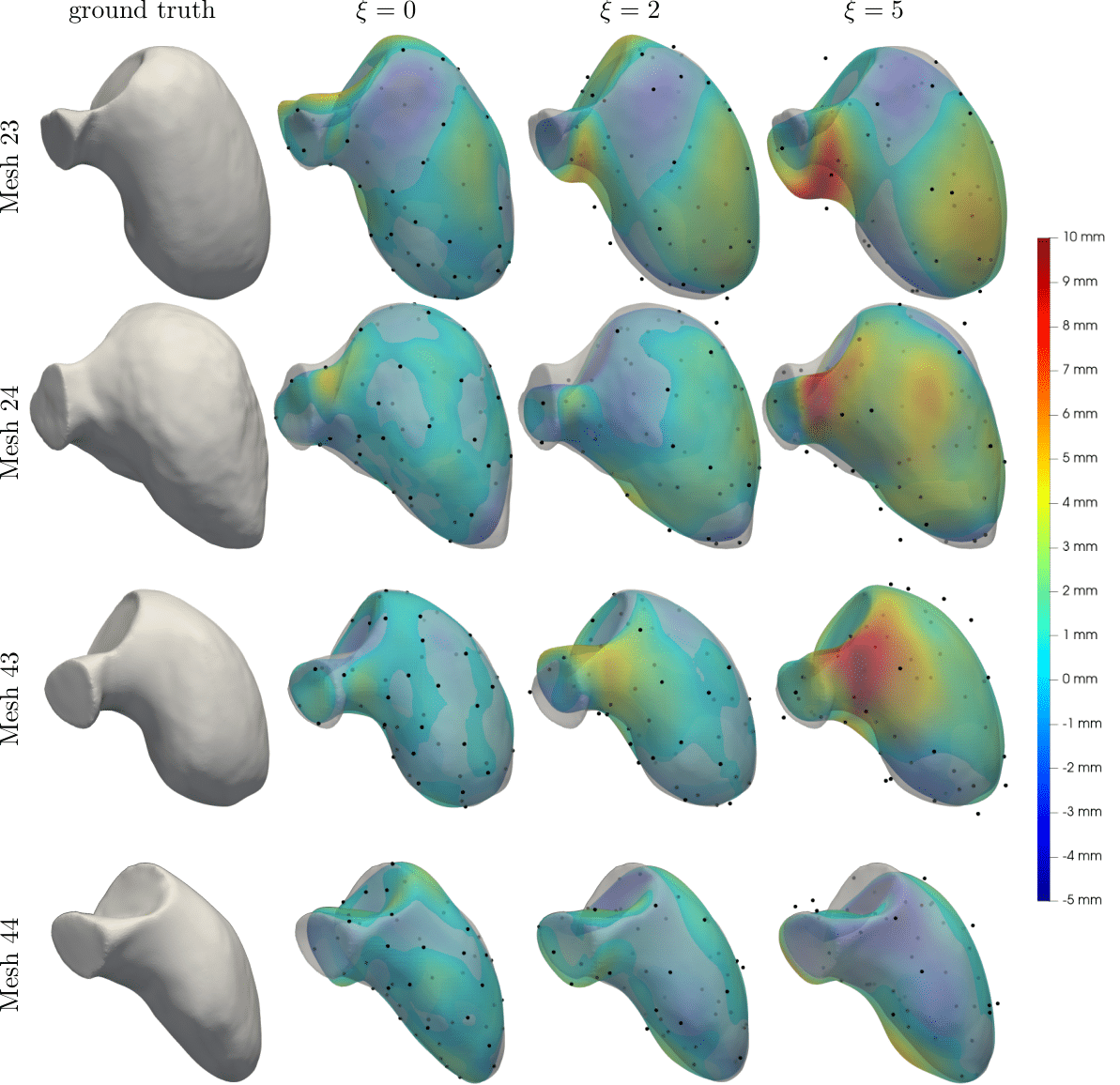
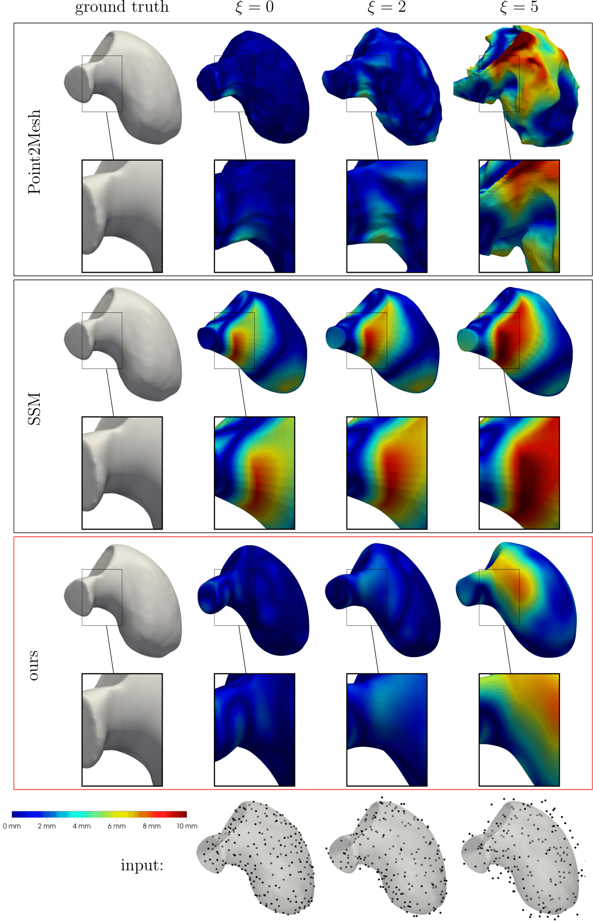
The performance of our method is compared with Points2Surf [24], Point2Mesh [19], and a fitted statistical shape model (SSM), based on the data in [35]. In all experiments, only points on the endocardium of the left ventricle are considered. All methods are compared on point clouds with different cardinalities $n$, ranging from very sparse point clouds with $n=50$ to relatively dense ones with $n=2000$. Additionally, the coordinates of the points are perturbed with noise drawn from a Gaussian normal distribution with zero mean and fixed covariance $\xi^{2}I$. For each number of points $n$ and level of noise $\xi$ we test the methods on the same 4-point clouds sampled from the meshes of the test set (for Points2Surf we apply a pre-trained model [24]). The statistical shape model describes a heart shape as a variation of a mean shape $\mu$ in different directions (modes). We used the publicly available SSM from the cardiac atlas project that is based on $630$ healthy Biobank reference patients, further described in [35]. A mean point cloud $\mathbf{X}\in\mathbb{R}^{N\times 3}$ of $N$ points together with 200 eigenmodes $\mathbf{V}_{i}\in\mathbb{R}^{N\times 3}$ for $i=1,\ldots,200$ and corresponding eigenvalues $\lambda\in\mathbb{R}^{200}$ are provided, which is restricted to the subset of points corresponding to the endocardium of the left ventricle. For a given sample with weights $\alpha\in\mathbb{R}^{200}$ and a spatial offset $\mathbf{b}\in\mathbb{R}^{3}$, we obtain a representation of the resulting point cloud $C$ as $\mathbf{C}=\mathbf{X}+\mathbf{1}_{N}\mathbf{b}^{\top}+\sum_{i=1}^{200}\alpha_{i}\lambda_{i}\mathbf{V}_{i}$. For a given target point cloud $\mathbf{Y}$ we use this model to optimize the asymmetric Chamfer distance $d_{\text{aCD}}(\mathbf{Y},\mathbf{C})=\frac{1}{|\mathbf{Y}|}\sum_{y\in\mathbf{Y}}\min_{x\in\mathbf{C}}\|x-y\|_{2}$ w.r.t. the weights $\alpha$ and the spatial offset $\mathbf{b}$. Additionally, we use a standard $\ell_{2}$ loss term to obtain the final objective function

$$\mathcal{J}_{\mathbf{Y}}(\alpha,\mathbf{b})=d_{\text{aCD}}\left(\mathbf{Y},\mathbf{X}+\mathbf{1}_{N}\mathbf{b}^{\top}+\sum_{i=1}^{200}\alpha_{i}\lambda_{i}\mathbf{V}_{i}\right)+\beta\|\alpha\|_{2}.$$

This loss function is optimized for 5 000 epochs with the Adam optimizer [49], with a learning rate of $0.005$. For our Lipschitz regularized DeepSDF we take $\beta=\max(1,C_{s}\xi^{2})$ and minimize the objective in (2) using the Adam optimizer [49] with a learning rate of $10^{-2}$ for 50 000 epochs. The results for $n=50$ on all four validation meshes of the test set computed with our method are depicted in Figure 5. For every test case, we state the mean and standard deviation across the four meshes of the test set for the above metrics in Table 1. Note that for Points2Surf did not converge for sparse point clouds ($n=50$ and $n=200$). We thus omitted the associated results in the table. Our method performs particularly well on sparse point clouds compared to the other methods. The obtained meshes are qualitatively similar to the ground truth meshes and geometric features like the curvature can be recovered properly, as can be seen in Figure 6.

4.5 Inference from electroanatomical mapping data

Figure 7: Reconstruction of the LV endocardium from the EAM data. We compare the SSM reconstruction (left panel) to our approach for an optimal noise level estimation of $\bar{\sigma}=3.368$ (right panel). We also report the absolute distance from the geometry provided by the EAM system.

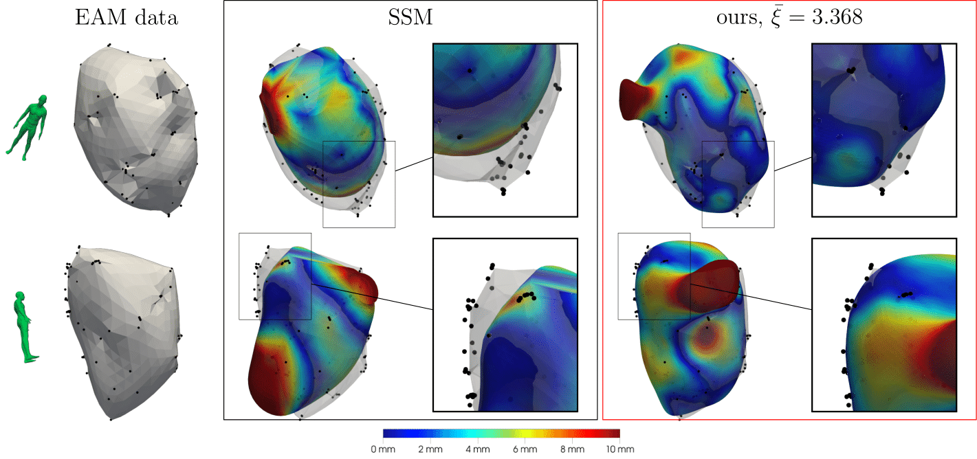
Electro-anatomical mapping (EAM) is commonly performed in patients undergoing catheter ablation. Our EAM data consist of a set of points located on the endocardial surface of the left ventricle, along with electrograms for each acquired point. The point cloud is usually sparse and unevenly distributed, but commonly allows for a reasonable estimate of endocardial geometry.

The EAM data has been acquired with the NOGA-XP system (Biologic Delivery Systems, Biosense Webster) equipped with a conventional 7-Fr deflectable-tip mapping catheter (NAVI-STAR, Biosense Webster). Spatial positions of the tip of the catheter were acquired at 100 Hz, and aligned in time using the automatically detected R-peak of the 12-lead ECG. Points were accepted by the system according to a set of criteria for catheter stability and signal quality. The institutional review board approved the study protocol, and all patients gave written and oral informed consent for the investigation (the study is compliant with the Declaration of Helsinki). Further information on the study has been previously reported [51, 52]. We pre-processed the data by applying a $-90^{\circ}$ rotation about the $X$-axis (NOGA to LPS-MRI coordinate system), followed by a translation to align the LV epicardial apex with the origin. Note that only an approximate alignment is possible since the epicardium is not present in the EAM data.

The results are reported in Figure 7. The overall LV shape is well-approximated, including the outflow aortic tract. Compared to the LV surface obtained from the EAM system, based on interpolation, our shape is much smoother and can extrapolate in regions where data is sparse or missing. Since the underlying noise structure is unknown, we estimate the noise variance iteratively as described in Equation 3. For the EAM data, we obtain an estimate of $3.4$ mm, consistent with the size of the electrode’s tip ($2-4$ mm). Additionally, the performance of this method is tested for a synthetic point cloud (Heart 43, $n=500$, $\xi=5$), where the correct noise level is obtained. We report the noise estimation iterates for the synthetic point cloud and the EAM data in Table 2.

step	synthetic		EAM data
$\bar{\xi}_{0}$	0	15	0	15
$\bar{\xi}_{1}$	3.159	4.882	1.499	4.672
$\bar{\xi}_{2}$	4.878	5.063	3.184	3.686
$\bar{\xi}_{3}$	5.063	5.060	3.344	3.398
$\bar{\xi}_{4}$	5.060	5.060	3.797	3.367
$\bar{\xi}_{5}$	5.060	5.060	3.410	3.364
$\bar{\xi}_{6}$	5.060	5.060	3.368	3.364

Table 2: Iteration of the variance estimation for the synthetic case (Heart 43, $n=500$, $\xi=5$) and the EAM data.

5 Discussion and Outlook

We have presented a novel method to represent cardiac anatomy based on signed-distance functions. The quantitative comparison with other methods shows that our approach can reconstruct the shape of hearts on a state-of-the-art level, especially for sparse and noisy data. In contrast to the methods we compared against, our approach does not require knowledge of the normals at each point of the point cloud. This knowledge however could be incorporated at the shape completion stage by fitting the normalized gradient of the SDF against the given normals.

The requirement of point clouds is a mixed blessing, as it requires an additional step to work on image input, but enables the algorithm to operate on different modalities on the other hand. Learning multiple SDFs with one network allows the generation of shapes based on input data from different chambers of the heart or a combination of multiple surfaces.

While the present work only encodes bi-ventricular surfaces, the method itself can be straightforwardly extended to encode additional chambers and shapes, such as the atria or aorta. This new methodology furthermore alleviates the generation of synthetic anatomical models through latent space interpolation. Additionally, this method is particularly well-suited for generating anatomical cohorts [2] and to provide a good prior for shape uncertainty quantification [53]. Finally, it also could offer a way to smoothly transfer quantities on the domain using optimal transport methods in the latent space.

References

- [1] Jorge Corral-Acero et al. “The ‘Digital Twin’ to enable the vision of precision cardiology” In European Heart Journal 41.48, 2020, pp. 4556–4564 DOI: 10.1093/eurheartj/ehaa159
- [2] Marina Strocchi et al. “A publicly available virtual cohort of four-chamber heart meshes for cardiac electro-mechanics simulations” Publisher: Public Library of Science In PLOS ONE 15.6, 2020, pp. e0235145 DOI: 10.1371/journal.pone.0235145
- [3] Nathan Painchaud, Youssef Skandarani, Thierry Judge, Olivier Bernard, Alain Lalande and Pierre-Marc Jodoin “Cardiac Segmentation With Strong Anatomical Guarantees” Conference Name: IEEE Transactions on Medical Imaging In IEEE Transactions on Medical Imaging 39.11, 2020, pp. 3703–3713 DOI: 10.1109/TMI.2020.3003240
- [4] Víctor M. Campello et al. “Multi-Centre, Multi-Vendor and Multi-Disease Cardiac Segmentation: The M&Ms Challenge” Conference Name: IEEE Transactions on Medical Imaging In IEEE Transactions on Medical Imaging 40.12, 2021, pp. 3543–3554 DOI: 10.1109/TMI.2021.3090082
- [5] Xiahai Zhuang et al. “Cardiac segmentation on late gadolinium enhancement MRI: A benchmark study from multi-sequence cardiac MR segmentation challenge” In Medical Image Analysis 81, 2022, pp. 102528 DOI: 10.1016/j.media.2022.102528
- [6] Deepak Bhakta and John M Miller “Principles of electroanatomic mapping” Publisher: Elsevier In Indian pacing and electrophysiology journal 8.1, 2008, pp. 32
- [7] Carlos Ruiz-Herrera, Thomas Grandits, Gernot Plank, Paris Perdikaris, Francisco Sahli Costabal and Simone Pezzuto “Physics-informed neural networks to learn cardiac fiber orientation from multiple electroanatomical maps” In Engineering with Computers, 2022 DOI: 10.1007/s00366-022-01709-3
- [8] Jeong Joon Park, Peter Florence, Julian Straub, Richard Newcombe and Steven Lovegrove “DeepSDF: Learning Continuous Signed Distance Functions for Shape Representation” arXiv: 1901.05103 In arXiv:1901.05103 [cs], 2019 URL: http://arxiv.org/abs/1901.05103
- [9] Hsueh-Ti Derek Liu, Francis Williams, Alec Jacobson, Sanja Fidler and Or Litany “Learning Smooth Neural Functions via Lipschitz Regularization” arXiv: 2202.08345 In arXiv:2202.08345 [cs], 2022 URL: http://arxiv.org/abs/2202.08345
- [10] Baorui Ma, Yu-Shen Liu, Matthias Zwicker and Zhizhong Han “Surface reconstruction from point clouds by learning predictive context priors” In Proceedings of the IEEE/CVF Conference on Computer Vision and Pattern Recognition, 2022, pp. 6326–6337
- [11] Jonathan C Carr et al. “Reconstruction and representation of 3D objects with radial basis functions” In Proceedings of the 28th annual conference on Computer graphics and interactive techniques, 2001, pp. 67–76
- [12] Michael Kazhdan, Matthew Bolitho and Hugues Hoppe “Poisson surface reconstruction” In Proceedings of the fourth Eurographics symposium on Geometry processing 7, 2006
- [13] Michael Kazhdan and Hugues Hoppe “Screened poisson surface reconstruction” In ACM Transactions on Graphics (ToG) 32.3 ACM New York, NY, USA, 2013, pp. 1–13
- [14] Benjamin Ummenhofer and Thomas Brox “Global, dense multiscale reconstruction for a billion points” In Proceedings of the IEEE international conference on computer vision, 2015, pp. 1341–1349
- [15] Simon Fuhrmann and Michael Goesele “Floating scale surface reconstruction” In ACM Transactions on Graphics (ToG) 33.4 ACM New York, NY, USA, 2014, pp. 1–11
- [16] Lars Mescheder, Michael Oechsle, Michael Niemeyer, Sebastian Nowozin and Andreas Geiger “Occupancy Networks: Learning 3D Reconstruction in Function Space” ISSN: 2575-7075 In 2019 IEEE/CVF Conference on Computer Vision and Pattern Recognition (CVPR), 2019, pp. 4455–4465 DOI: 10.1109/CVPR.2019.00459
- [17] Mateusz Michalkiewicz, Jhony K Pontes, Dominic Jack, Mahsa Baktashmotlagh and Anders Eriksson “Deep level sets: Implicit surface representations for 3d shape inference” In arXiv preprint arXiv:1901.06802, 2019
- [18] Zhiqin Chen and Hao Zhang “Learning implicit fields for generative shape modeling” In Proceedings of the IEEE/CVF Conference on Computer Vision and Pattern Recognition, 2019, pp. 5939–5948
- [19] Rana Hanocka, Gal Metzer, Raja Giryes and Daniel Cohen-Or “Point2Mesh: A Self-Prior for Deformable Meshes” In ACM Trans. Graph. 39.4 Association for Computing Machinery, 2020 DOI: 10.1145/3386569.3392415
- [20] Amos Gropp, Lior Yariv, Niv Haim, Matan Atzmon and Yaron Lipman “Implicit Geometric Regularization for Learning Shapes”, 2020 arXiv:2002.10099 [cs.LG]
- [21] Rohan Chabra et al. “Deep local shapes: Learning local sdf priors for detailed 3d reconstruction” In Computer Vision–ECCV 2020: 16th European Conference, Glasgow, UK, August 23–28, 2020, Proceedings, Part XXIX 16, 2020, pp. 608–625 Springer
- [22] Chiyu Jiang, Avneesh Sud, Ameesh Makadia, Jingwei Huang, Matthias Nießner and Thomas Funkhouser “Local implicit grid representations for 3d scenes” In Proceedings of the IEEE/CVF Conference on Computer Vision and Pattern Recognition, 2020, pp. 6001–6010
- [23] Edgar Tretschk, Ayush Tewari, Vladislav Golyanik, Michael Zollhöfer, Carsten Stoll and Christian Theobalt “Patchnets: Patch-based generalizable deep implicit 3d shape representations” In Computer Vision–ECCV 2020: 16th European Conference, Glasgow, UK, August 23–28, 2020, Proceedings, Part XVI 16, 2020, pp. 293–309 Springer
- [24] Philipp Erler, Paul Guerrero, Stefan Ohrhallinger, Niloy J. Mitra and Michael Wimmer “Points2Surf Learning Implicit Surfaces from Point Clouds” In Computer Vision – ECCV 2020 Springer International Publishing, 2020, pp. 108–124 DOI: 10.1007/978-3-030-58558-7_7
- [25] Ma Baorui, Han Zhizhong, Liu Yu-Shen and Zwicker Matthias “Neural-Pull: Learning Signed Distance Functions from Point Clouds by Learning to Pull Space onto Surfaces” In International Conference on Machine Learning (ICML), 2021
- [26] Julian Chibane and Gerard Pons-Moll “Neural unsigned distance fields for implicit function learning” In Advances in Neural Information Processing Systems 33, 2020, pp. 21638–21652
- [27] Olivier Ecabert et al. “Automatic Model-Based Segmentation of the Heart in CT Images” In IEEE Transactions on Medical Imaging 27.9, 2008, pp. 1189–1201 DOI: 10.1109/TMI.2008.918330
- [28] Corné Hoogendoorn et al. “A High-Resolution Atlas and Statistical Model of the Human Heart From Multislice CT” In IEEE Transactions on Medical Imaging 32.1, 2013, pp. 28–44 DOI: 10.1109/TMI.2012.2230015
- [29] J. Lötjönen, S. Kivistö, J. Koikkalainen, D. Smutek and K. Lauerma “Statistical shape model of atria, ventricles and epicardium from short- and long-axis MR images” Medical Image Computing and Computer-Assisted Intervention - MICCAI 2003 In Medical Image Analysis 8.3, 2004, pp. 371–386 DOI: https://doi.org/10.1016/j.media.2004.06.013
- [30] Sebastian Ordas, Estanislao Oubel, Rafael Sebastian and Alejadro F. Frangi “Computational Anatomy Atlas of the Heart” In 2007 5th International Symposium on Image and Signal Processing and Analysis, 2007, pp. 338–342 DOI: 10.1109/ISPA.2007.4383715
- [31] Mathias Unberath, Andreas Maier, Dominik Fleischmann, Joachim Hornegger and Rebecca Fahrig “Open-source 4D statistical shape model of the heart for x-ray projection imaging” In 2015 IEEE 12th International Symposium on Biomedical Imaging (ISBI), 2015, pp. 739–742 DOI: 10.1109/ISBI.2015.7163978
- [32] Xiahai Zhuang, Kawal S. Rhode, Reza S. Razavi, David J. Hawkes and Sebastien Ourselin “A Registration-Based Propagation Framework for Automatic Whole Heart Segmentation of Cardiac MRI” In IEEE Transactions on Medical Imaging 29.9, 2010, pp. 1612–1625 DOI: 10.1109/TMI.2010.2047112
- [33] Claudia Nagel, Steffen Schuler, Olaf Dössel and Axel Loewe “A bi-atrial statistical shape model for large-scale in silico studies of human atria: Model development and application to ECG simulations” In Medical Image Analysis 74, 2021, pp. 102210 DOI: https://doi.org/10.1016/j.media.2021.102210
- [34] W Bai et al. “A bi-ventricular cardiac atlas built from 1000+ high resolution MR images of healthy subjects and an analysis of shape and motion” In Med Image Anal. 26.1 Oxford University Press, 2015, pp. 133–45 DOI: 10.1016/j.media.2015.08.009
- [35] Steffen E. Petersen et al. “Reference ranges for cardiac structure and function using cardiovascular magnetic resonance (CMR) in Caucasians from the UK Biobank population cohort” In Journal of Cardiovascular Magnetic Resonance 19.1, 2017, pp. 18 DOI: 10.1186/s12968-017-0327-9
- [36] Marcel Beetz, Abhirup Banerjee and Vicente Grau “Point2Mesh-Net: Combining Point Cloud and Mesh-Based Deep Learning for Cardiac Shape Reconstruction” In Statistical Atlases and Computational Models of the Heart. Regular and CMRxMotion Challenge Papers: 13th International Workshop, STACOM 2022, Held in Conjunction with MICCAI 2022, Singapore, September 18, 2022, Revised Selected Papers, 2023, pp. 280–290 Springer
- [37] Dieuwertje Alblas, Christoph Brune, Kak Khee Yeung and Jelmer M Wolterink “Going Off-Grid: Continuous Implicit Neural Representations for 3D Vascular Modeling” In Statistical Atlases and Computational Models of the Heart. Regular and CMRxMotion Challenge Papers: 13th International Workshop, STACOM 2022, Held in Conjunction with MICCAI 2022, Singapore, September 18, 2022, Revised Selected Papers, 2023, pp. 79–90 Springer
- [38] Marcel Beetz et al. “Interpretable cardiac anatomy modeling using variational mesh autoencoders” In Frontiers in Cardiovascular Medicine 9, 2022 DOI: 10.3389/fcvm.2022.983868
- [39] Fanwei Kong, Nathan Wilson and Shawn Shadden “A deep-learning approach for direct whole-heart mesh reconstruction” In Medical Image Analysis 74, 2021, pp. 102222 DOI: https://doi.org/10.1016/j.media.2021.102222
- [40] Zhaohan Xiong et al. “Automatic 3D Surface Reconstruction of the Left Atrium From Clinically Mapped Point Clouds Using Convolutional Neural Networks” In Frontiers in Physiology 13, 2022 DOI: 10.3389/fphys.2022.880260
- [41] Cristobal Rodero et al. “Virtual cohort of adult healthy four-chamber heart meshes from CT images” Type: dataset Zenodo, 2021 DOI: 10.5281/zenodo.4590294
- [42] Marina Strocchi et al. “A Publicly Available Virtual Cohort of Four-chamber Heart Meshes for Cardiac Electro-mechanics Simulations” Type: dataset Zenodo, 2020 DOI: 10.5281/zenodo.3890034
- [43] Jason Bayer et al. “Universal ventricular coordinates: A generic framework for describing position within the heart and transferring data” In Medical Image Analysis 45, 2018, pp. 83–93 DOI: 10.1016/j.media.2018.01.005
- [44] Thomas Grandits “A Fast Iterative Method Python package” In Journal of Open Source Software 6.66, 2021, pp. 3641 DOI: 10.21105/joss.03641
- [45] Will Schroeder, Ken Martin and Bill Lorensen “The Visualization Toolkit (4th ed.)” Kitware, 2006
- [46] C. Sullivan and Alexander Kaszynski “PyVista: 3D plotting and mesh analysis through a streamlined interface for the Visualization Toolkit (VTK)” In Journal of Open Source Software 4.37 The Open Journal, 2019, pp. 1450 DOI: 10.21105/joss.01450
- [47] Tingran Gao, Shahar Z. Kovalsky and Ingrid Daubechies “Gaussian Process Landmarking on Manifolds” Publisher: Society for Industrial and Applied Mathematics In SIAM Journal on Mathematics of Data Science 1.1, 2019, pp. 208–236 DOI: 10.1137/18M1184035
- [48] Michael Dawson-Haggerty et al. “trimesh” URL: https://trimsh.org/
- [49] Diederik P Kingma and Jimmy Ba “Adam: A method for stochastic optimization” In The International Conference on Learning Representations (ICLR), 2015
- [50] Blender Online Community “Blender - a 3D modelling and rendering package”, 2018 Blender Foundation URL: http://www.blender.org
- [51] Francesco Maffessanti et al. “The influence of scar on the spatio-temporal relationship between electrical and mechanical activation in heart failure patients” In EP Europace 22.5 Oxford University Press, 2020, pp. 777–786 DOI: 10.1093/europace/euz346
- [52] Simone Pezzuto et al. “Reconstruction of three-dimensional biventricular activation based on the 12-lead electrocardiogram via patient-specific modelling” In EP Europace 23.4 Oxford University Press, 2021, pp. 640–647 DOI: 10.1093/europace/euaa330
- [53] Lia Gander, Rolf Krause, Michael Multerer and Simone Pezzuto “Space-time shape uncertainty in the forward and inverse problem of electrocardiography” In International Journal for Numerical Methods in Biomedical Engineering 37, 2021 DOI: 10.1002/cnm.3522