Comparing Rapid Type Analysis with Points-To Analysis in GraalVM Native Image

Abstract.

Whole-program analysis is an essential technique that enables advanced compiler optimizations. An important example of such a method is points-to analysis used by ahead-of-time (AOT) compilers to discover program elements (classes, methods, fields) used on at least one program path. GraalVM Native Image uses a points-to analysis to optimize Java applications, which is a time-consuming step of the build. We explore how much the analysis time can be improved by replacing the points-to analysis with a rapid type analysis (RTA), which computes reachable elements faster by allowing more imprecision. We propose several extensions of previous approaches to RTA: making it parallel, incremental, and supporting heap snapshotting. We present an extensive experimental evaluation of the effects of using RTA instead of points-to analysis, in which RTA allowed us to reduce the analysis time for Spring Petclinic—a popular demo application of the Spring framework—by 64 % and the overall build time by 35 % at the cost of increasing the image size due to the imprecision by 15 %.

1. Introduction

Whole-program analysis is an essential technique enabling advanced compiler optimizations. An important example of such a technique is points-to analysis (PTA) (Hind, 2001; Ryder, 2003; Smaragdakis and Balatsouras, 2015; Sridharan et al., 2013) used to discover program elements (classes, methods, fields) that are used in at least one run of the program and hence need to be compiled. We call such elements reachable.

GraalVM Native Image (Wimmer et al., 2019) combines PTA, application initialization at build time, heap snapshotting, and ahead-of-time (AOT) compilation to optimize Java applications. This combination of features reduces the application startup time and memory footprint. Without using PTA, everything on the Java class path would have to be compiled. That would lead to long build times and unnecessary large binaries (Wimmer et al., 2019). The results of the PTA are thus essential, but the overhead of computing points-to sets for each variable is significant. It can take minutes to analyze big applications.

Long build times are inconvenient for developers because they are used to compiling their applications often, and any delay can significantly hurt their productivity. To give a concrete example from our later presented experiments, we can mention a larger web application (the Spring Petclinic) where the analysis takes 159 seconds. We explore how much time can be saved by using a rapid type analysis (RTA) (Bacon and Sweeney, 1996; Sundaresan et al., 2000) instead of PTA. Intuitively, the basic idea of RTA is to discover which types, i.e., classes from a given class hierarchy, can be used in methods so-far known to be reachable from given root methods, which can in turn enlarge the set of reachable methods by considering that any so-far instantiated type can appear in a variable of a certain super-type, leading to an iterative fixed point computation.

We show how the above idea can be applied in the context of GraalVM Native Image where one has to deal with issues such as heap snapshotting. We build on similar principles as B. Tizer in (Titzer, 2006). On top of that, we also develop a parallel and incremental version of the analysis. The incrementality is achieved by using method summaries that sum up the effect of each analyzed method. These summaries can be serialized and reused between multiple builds.

RTA can provide results quicker at the cost of reduced precision. The lower precision can yield bigger binaries, which is not so problematic during the development phase. On the other hand, the need to compile more classes and methods goes against the savings due to the cheaper analysis. We try to answer the research question whether such a loss of precision is justified. We perform an extensive experimental comparison of our version of RTA and the PTA currently implemented in GraalVM Native Image to see whether RTA can provide some advantage over the PTA, and if so, how much.

For our experiments, we use the standard Java benchmark suites Renaissance (Prokopec et al., 2019) and Dacapo (Blackburn et al., 2006) along with example applications for the Java microservice frameworks Spring (VMWare, 2023), Micronaut (Micronaut foundation, 2023), and Quarkus (RedHat, 2023). The experimental evaluation shows, for example, that RTA can reduce the analysis time of Spring Petclinic—a popular demo application of the Spring framework—by 64 % and the overall build time by 35 % at the cost of increasing the image size by 15 %. On average, RTA reduced the analysis time by 40 % and the overall build time by 15 % at the cost of increasing the image size by 15 %.

We also experiment with the scalability of both RTA and PTA with respect to the number of available processor cores. The results show that, for a reduced number of threads, such as 1 or 4, the savings in analysis time can be even greater, making RTA a good choice for constrained environments such as GitHub Actions (git, 2022) or similar CI pipelines.

Our implementation, which is based on the Native Image component of GraalVM (Oracle, 2023a), is written in Java and Java is used for all examples in this paper. However, our approach is not limited to Java or languages that compile to Java bytecode. It can be applied to all managed languages that are amenable to points-to analysis, such as C# or other languages of the .NET framework.

In summary, this paper contributes the following:

• We introduce a new variant of rapid type analysis for the context of GraalVM Native Image. It supports class initialization at build time and heap snapshotting.

• We extend the proposed algorithm to be parallel and incremental. The incrementality is achieved by using method summaries that sum up the effect of each analyzed method. These summaries can be serialized and reused between multiple builds.

• We provide a detailed comparison of the new variant of RTA with a points-to analysis for ahead-of-time compilation of Java. We discuss the effects on analysis time, build time, reachable elements, and binary size. We also evaluate the scalability of both analysis methods. The results show that for bigger applications the analysis time can be reduced by up to 64 %.

2. Overview of GraalVM Native Image

GraalVM Native Image (Wimmer et al., 2019) produces standalone binaries for Java applications that contain the application along with all dependencies and necessary runtime components such as the garbage collector and threading support. It relies on a closed-world assumption, i.e., all code is available to analyze at image build time. Dynamic features such as reflection and dynamic class loading are supported by explicitly registering the program elements that would otherwise be opaque to the analysis. The image build process consists of several successive phases and subphases.

First, the points-to analysis is started to detect reachable program elements. It starts with a set of root methods, which includes the application entry point specified by the user as well as the entry points of runtime components. The execution of the analysis is interconnected with application initialization and heap snapshotting.

Application initialization at build time allows developers to initialize parts of their application when the image is being built instead of performing the initialization at every application startup. During the initialization, static fields of initialized classes are assigned to either manually written or default values. Heap snapshotting traverses all the objects reachable from static fields of the initialized classes and constructs an object graph, i.e., a directed graph of instances whose edges are references to other objects reachable via instance fields or array slots. The object graph constitutes the image heap and is stored as a part of the binary file. When the application is started, the image heap is mapped directly into memory (Wimmer et al., 2019). This process and its interaction with static analysis are discussed in more details in Section 3.5.

After the analysis finishes, the ahead-of-time compilation is started. We use the Graal Compiler for compilation. Methods are represented using the Graal Intermediate Representation (IR), which is graph-based and models both the control-flow and the data-flow dependencies between nodes (Stadler et al., 2013). At this point, the IR graphs are optimized using the facts proven by the analysis. Finally, the image heap and compiled code are written into the image file.

2.1. Points-to Analysis in GraalVM Native Image

This section presents the points-to analysis used in GraalVM Native Image, which was introduced in (Wimmer et al., 2019). The analysis is context-insensitive, path-sensitive, flow-insensitive for fields but flow-sensitive for local variables. It starts with a set of root methods and iteratively processes all transitively reachable methods until a fixed-point is reached.

During the analysis, objects are represented by their types only, not by their allocation sites as is common in other pointer analyses (Smaragdakis and Balatsouras, 2015). Using the type abstraction is a sufficiently powerful approximation which yields good results in practice when the goal is to compute reachable program elements, while keeping the analysis time reasonably low. This type information is enough to enable compiler optimizations such as virtual method de-virtualization.

Each reachable method is parsed from bytecode into the Graal IR, which is then transformed into a type-flow graph. Nodes of type-flow graphs include those representing instructions as well as nodes representing formal parameters and return values of methods. The nodes are connected via directed use edges.

Each node maintains a type-state information about all types that can reach it. Allocation nodes, i.e., nodes representing allocation instructions, act as sources that produce types, which are then propagated along the use edges (with the input/output of nodes representing method invocations handled in a different way as discussed below). Once a type is added to a type-state, it is never removed. Thus, the size of all type states can only grow. In any compilation run, the number of program elements (classes, methods, and fields) is given and finite. As the number of reachable elements only grows during the analysis and there is a fixed upper-bound, termination is guaranteed. The worst-case scenario happens when all program elements are reachable by the analysis.

Type-flow graphs of methods are connected into a single interprocedural graph covering the whole application. For that, nodes producing arguments of method calls are connected with formal-parameters nodes of the target methods, and return nodes from the target methods are connected back into the invocation nodes in the callers. The input edges of invocation nodes are thus not used for regular type propagation but rather for steering the interconnection of sources of arguments with the formal-parameter nodes (and of the appropriate return node with the invocation node).

For static methods, this linkage happens when the type-flow of the caller is created. For virtual methods, the linkage happens dynamically during the analysis. Every time a new type is added into the type-state of a receiver of a method call, it is used to resolve, i.e., to identify, the concrete method to be linked.

To better understand our PTA, let us now walk through an example. For brevity, we omit calls to constructors and exception handling. Consider the program in Figure 1. The analysis starts with the entry point Hello.main(). The method is parsed, and the type-flow graph in Figure 2 created. It contains the following nodes:

• An invocation node $\mathit{in}_{1}$ for the call of foo().

• An allocation node $\mathit{an}_{1}$ for Hello, connected to $in_{1}$ as a source of receiver types of the call of foo().

• An allocation node $\mathit{an}_{2}$ for A, connected to $\mathit{in}_{1}$ as a source of argument types in the call of foo().

• An invocation node $\mathit{in}_{2}$ for the call of log().

Since $\mathit{an}_{1}$ is used by $\mathit{in}_{1}$ as a source of its receiver types and since the invocation is virtual, as soon as the type Hello appears in $\mathit{an}_{1}$, the resolution of virtual methods is used, and Hello.foo() is found as the method to be invoked. The body of Hello.foo() is parsed and transformed into the corresponding type-flow graph with the following nodes:

• A formal-parameter node $\mathit{fn}_{1}$ used as a source of types of the implicit this parameter.

• A formal-parameter node $\mathit{fn}_{2}$ used as a source of types of the formal parameter i.

• An invocation node $\mathit{in}_{3}$ for the call of bar() that uses $\mathit{fn}_{2}$ as a source of its receiver types.

Now, $\mathit{an}_{1}$ and $\mathit{an}_{2}$ get connected to $\mathit{fn}_{1}$ and $\mathit{fn}_{2}$, resp., allowing a flow of types from Hello.main() into Hello.foo(). The type A can hence flow from $\mathit{an}_{2}$ to $\mathit{fn}_{2}$ and be used as a receiver type of $\mathit{in}_{3}$ that is constructed for the call I.bar(), upon which the resolution selects A.bar() as the call target.

The call to Hello.log() is static, and so its target can be determined directly. Its type flow-graph contains an allocation node $\mathit{an}_{3}$ of B. Note that while the type B is instantiated, its method B.bar() is not considered reachable as $\mathit{an}_{3}$ has no use edge, and so it can never flow out of the method and get into the invocation node of I.bar() in Hello.foo().

⬇

public class Hello {

public static void main() {

new Hello().foo(new A());

log();

}

static void log() { new B(); }

void foo(I i) { i.bar(); }

}

interface I { void bar(); }

class A implements I {...}

class B implements I {...}

Figure 1. Running example for analysis.

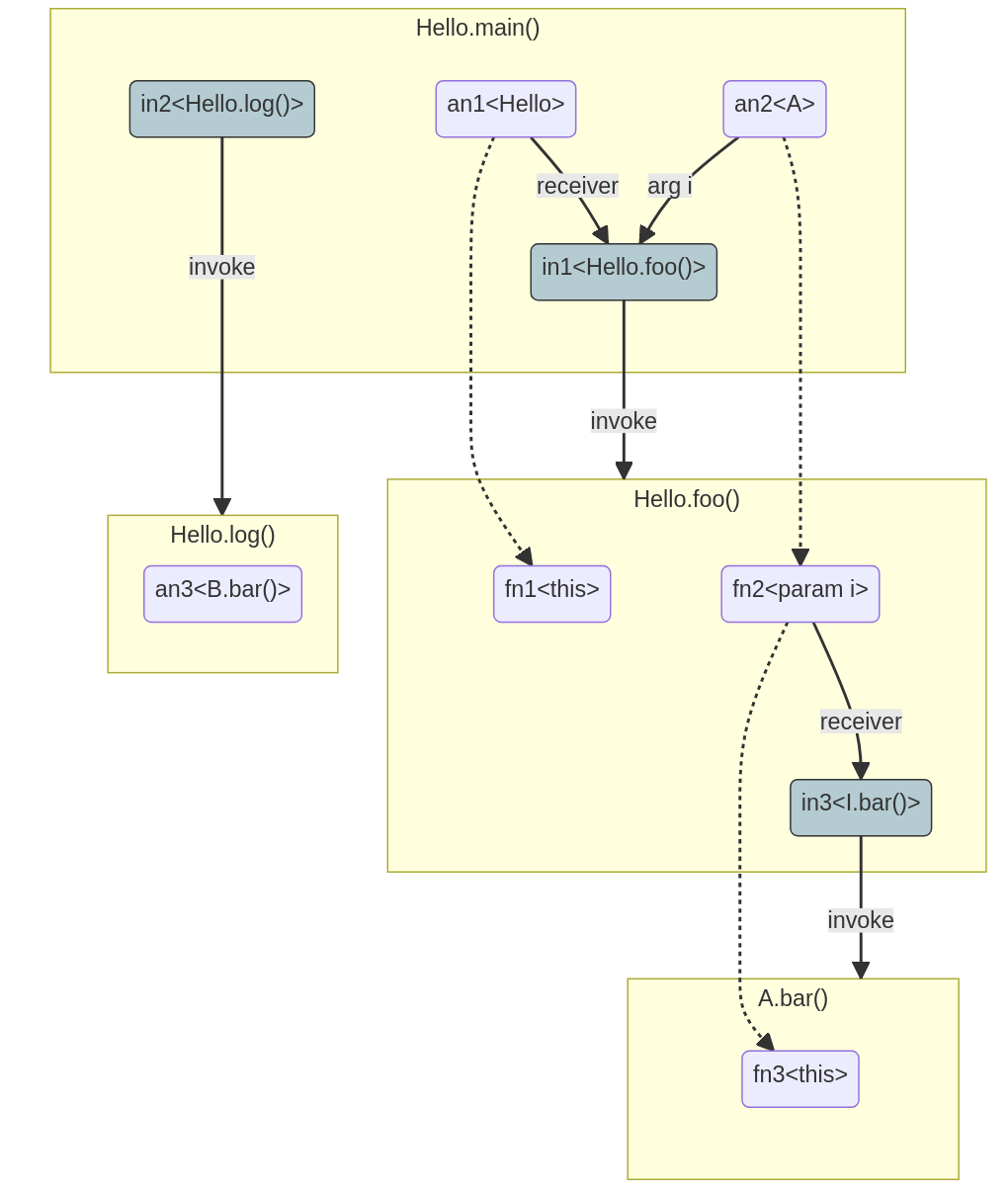
Figure 2. Running example type-flow graph.

The results of the points-to analysis are useful not only to identify reachable elements but also for many compiler optimizations. For example, they can be used to remove unnecessary casts, remove dead branches of instanceof checks that are always true or false, exclude fields that are never accessed, and to optimize virtual calls with a limited number of receiver types. Knowing the set of receivers and their types allows one to devirtualize method calls with only one receiver type, employ polymorphic inline caching (Hölzle et al., 1991) when there are a few receiver types only, and perform more method inlining, which can lead to subsequent optimizations.

3. RTA with Method Summaries

This section presents our implementation of RTA (Bacon and Sweeney, 1996; Sundaresan et al., 2000). It supports heap snapshotting, is designed to be parallel, and supports method summaries to make it incremental. First, we describe the basic idea of the core of the analysis using a system of high-level constraints, which neglects some more technical aspects of the actual analysis to be easier to understand. Then, we describe a single-threaded, non-incremental version of the proposed analysis, which, however, already contains some preparation for its subsequent parallelization. Afterwards, we propose how to run parts of the analysis in parallel, and, finally, we discuss incremental analysis.

The basic effect of the analysis—assuming all method calls to be virtual (i.e., not distinguishing different types of invocations)—can be summarized using the following constraints inspired by the work of Tip et al. in (Tip and Palsberg, 2000).

Let $T$ be the set of all types, $M$ the set of all methods, and $E$ the set of all expressions in the analyzed application. We use $StaticType(e)$ to denote the static type of $e\in E$. Furthermore, $Subtypes(t)$ denotes the set of all subtypes of $t\in T$, and $StaticLookup(t,m)$ denotes the actual call target for a virtually invoked $m\in M$ on $t\in T$. For $m\in M$, let $CallExpr(m)$ denote the set of all call expressions $e.f()$ for $e\in E$ and $f\in M$ that appear in the method $m$, and let $InstExpr(m)$ denote the set of all instantiation expressions $\mathtt{new}\,C()$ for $C\in T$ that appear in $m$. The sets $R\subseteq M$ and $I\subseteq T$ representing reachable methods and instantiated types determined using RTA satisfy the following constraints:

1. $\mathtt{main}\in R$.

2. $\forall m\in R~{}\forall e.f()\in CallExpr(m)\\ \forall t\in Subtypes(StaticType(e)).$
   $t\in I\land StaticLookup(t,f)=m^{\prime}\implies m^{\prime}\in R$.

3. $\forall m\in R~{}\forall new\,C()\in InstExpr(m).~{}C\in I$.

Intuitively, $\mathtt{main}$ is always reachable. The second rule makes sure that all methods that can be virtually called from a call expression in a reachable method are also reachable. Finally, the third rule makes sure that any type that can be instantiated in a reachable method is considered instantiated.

The above constraints showed how RTA handles virtual method invocations. However, there are actually five different types of invokes in Java: invokestatic, invokevirtual, invokeinterface, invokespecial, and invokedynamic.

As defined in the JVM specification (Lindholm et al., 2023), invokevirtual and invokeinterface represent virtual method invocations, and we do not need to distinguish them for our purposes. Invokestatic represents static method invocation, i.e., a direct invocation of a method called on a Java class, not on an instance. Invokespecial represents a direct invocation of an instance method in cases where it is clear which method should be called. This instruction is used, for example, when calling constructors, when calling a method on the superclass of the current class, or when calling a method on an expression of a type that has no subtypes. Both invokestatic and invokespecial are direct invokes, i.e. they have a unique call target that can be statically determined. Therefore, they could be resolved in the same way immediately upon the discovery of the invoke instruction in the bytecode of any reachable method. However, as shown in Section 3.3, differentiating between them can actually increase the precision in some cases. Invokedynamic represents a special invoke whose call target is not yet fixed but computed on the first execution of the bytecode. As our analysis is based on the Graal IR, it does not have to handle invokedynamic explicitly because these invokes are processed by the Graal compiler before the analysis starts and are optimized either into direct invokes or into lookup procedures determining the correct call target at runtime.

3.1. Core Algorithm and Data Structures

We now refine the above presented basic idea of RTA such that (1) it takes into account different kinds of calls that can appear (static calls, virtual calls, special calls), (2) computes information needed for subsequent compilation phases (in order not to have to repeat the analysis for this purpose), and (3) is ready for subsequent parallelization.

During the analysis, the effect of each method is represented using a method summary that consists of sets that contain the following information: static invoked methods, virtually invoked methods, special invoked methods, instantiated types, read fields, written fields, and embedded constants. The summary format is designed to be minimal while still containing all the necessary information for both RTA and the later AOT compilation step. For example, distinguishing between read and written fields is not needed for RTA itself, but AOT compilation requires the information since it automatically removes never accessed fields (Wimmer et al., 2019). The information about which fields are read is also needed to drive the heap snapshotting (cf. Section 3.5).

The internal state of the analysis can be viewed as consisting of a worklist containing all methods that still need to be analyzed and the following pieces of information associated with the representation kept by the compiler for types, methods, and fields:

• For each type t, the analysis stores the following:

  • An atomic boolean flag set to true if the analysis discovers that $t$ may be instantiated at run time.

  • A set of methods declared in t that the analysis has so-far found to be virtually invoked.

  • A set of methods declared in t that the analysis has so-far found to be special invoked.

  • A set of subtypes of t discovered as instantiated.

• For each method m, the analysis stores the following:

  • An atomic boolean flag marking $m$ as invoked, indicating that the method body is considered reachable at runtime.

  • An atomic boolean flag marking $m$ as special invoked, indicating that the method may be a target of an invoke special call.

  • An atomic boolean flag marking $m$ as virtually invoked, which indicates that the method may be the target of a virtual method call. Note that this does not necessarily mean that $m$ is invoked since the invoked method can come from some subtype of the declaring type of $m$.

• For each field f, the analysis stores the following:

  • An atomic boolean flag marking $f$ as read.

  • An atomic boolean flag marking $f$ as written.

The pseudocode of the core of the analysis can be found in Algorithm 1. It starts with a set of root methods used to initialize the worklist (line 1). The main loop (lines 2–7) then processes methods in the worklist until it becomes empty.

For each method in the worklist, it is first parsed into the Graal IR, the intermediate representation discussed previously (line 4). The summary of the method being processed is initialized to consist of empty sets. The extractSummary method (line 5) then iterates over the instructions of the method, and whenever it finds an instruction of the types listed in the left column of Table 1, it adds it to the collection of the summary given in the right column.

Table 1. Correspondence between bytecode instructions and collections in method summaries.

Bytecode instruction	Collection in the summary
new	Instantiated types
anewarray	Instantiated types
multianewarray	Instantiated types
getfield	Read fields
putfield	Written types
invoke*	Directly/Virtually called methods

When the summary is ready, it is passed into the appplySummary method (lines 9–20). This method iterates over all collections within the summary and calls appropriate register methods.

Many of the register methods are relatively straightforward. For example, see the method registerAsInvoked (lines 22–26), which adds an invoked method to the worklist. Note that the mark method (line 23) is called before adding the method being processed into the worklist. The mark method accepts a boolean flag as a parameter. If the flag is true, mark returns false (intuitively, no marking was needed). If the flag is false, mark atomically changes it to true and returns true (intuitively, the marking was needed). Hence, mark returns true only on its first invocation and false otherwise. This implementation with the atomic update is used to facilitate the parallel analysis presented later on. Registering fields as read or written follows the same pattern, and is omitted from the algorithm for space reasons.

3.2. Invoke Virtual Handling

The handling of virtual invokes and instantiated types is more interesting (see Algorithm 2). The two methods presented in the algorithm are interconnected.

The registerAsVirtualInvoked method (lines 1–11) handles a virtual method call. Since the analysis has no points-to information, it uses the declaring class of the invoked method to traverse all its currently instantiated subtypes. The information about instantiated subtypes is collected inside the registerAsInstantiated method (line 16). For each instantiated subtype, the virtual method is resolved into a concrete method using type.resolveMethod (line 7), which resolves a virtual call or interface call for the given concrete caller type according to the Java VM specification (Lindholm et al., 2023).

The registerAsInstantiated method (lines 13–26) is used when a type is instantiated. First, the newly instantiated type is added to the instantiatedSubytpes set of all supertypes. Then the supertype hierarchy is traversed again, and for each visited type, the list of all virtually invoked methods is processed (lines 20–23). This list is collected as a part of registerAsVirtualInvoked (line 4). For each virtually invoked method in the list, type.resolveMethod is used to obtain the concrete method (line 21).

Note that essentially the same method resolution is performed by both registerAsVirtualInvoked and registerAsInstantiated but from two different perspectives. It is not possible to have only one of them. That would require an ordering in which the register methods that only mark elements are called before the register methods that do the resolution. Such an ordering is not possible because discovering instantiated types and invoked methods is interconnected. Discovering new instantiated types makes new methods reachable from invokes within already analyzed methods and vice versa.

Input: The set of root methods

Output: All reachable types, methods, and fields

1:$worklist\leftarrow rootMethods$

2:while $worklist\neq\emptyset$ do

3:     $method\leftarrow removeFirst(worklist)$

4:     $irGraph\leftarrow parseMethod(method)$

5:     $summary\leftarrow extractSummary(irGraph)$

6:     $applySummary(summary)$

7:end while

8:procedure applySummary($summary$)

9:     for $m\leftarrow summary.directInvokes$ do

10:         $registerAsInvoked(m)$

11:     end for

12:     for $m\leftarrow summary.virtualInvokes$ do

13:         $registerAsVirtualInvoked(m)$

14:     end for

15:     for $t\leftarrow summary.instantiatedTypes$ do

16:         $registerAsInstantiated(t)$

17:     end for

18:     $//\;...\;similar\;loops\;for\;other\;parts\;...$

19:end procedure

20:procedure registerAsInvoked($m$)

21:     if $mark(m.isInvoked)$ then

22:         $worklist.add(m)$

23:     end if

24:end procedure

25:procedure mark($flag$)

26:     return $flag.compareAndSet(false,true)$

27:end procedure

Algorithm 1 Rapid type analysis worklist loop.

1:procedure registerAsVirtualInvoked($m$)

2:     if $mark(m.isVirtualInvoked)$ then

3:         $t\leftarrow m.declaringType$

4:         $t.virtualInvokedMethods.add(m)$

5:         for $subt\in t.instantiatedSubtypes$ do

6:              $resolved\leftarrow subt.resolveMethod(m)$

7:              $registerAsInvoked(resolved)$

8:         end for

9:     end if

10:end procedure

11:procedure registerAsInstantiated($t$)

12:     if $mark(t.isInstantiated)$ then

13:         for $supert\in t.superTypes$ do

14:              $supert.instantiatedSubtypes.add(t)$

15:         end for

16:         for $supert\in t.superTypes$ do

17:              for $m\in supert.virtualInvokedMethods$ do

18:                  $resolved\leftarrow t.resolveMethod(m)$

19:                  $registerAsInvoked(resolved)$

20:              end for

21:         end for

22:     end if

23:end procedure

Algorithm 2 RTA handling of virtual methods.

3.3. Invoke Special Handling

Another interesting case that we would like to discuss is invokespecial. Differentiating static invokes and special invokes is not necessary for correctness. However, it increases precision because there are cases when a special invoke is reachable, but no object is instantiated on which such method can be called. This happens, for example, when analyzing the method java.lang.Thread.sleep. A simplified version of the method for Java 20 can be found in Figure 3. It contains the handling of virtual threads from the project Loom (pro, 2023) (instances of VirtualThread) although their usage has to be explicitly enabled by a command line option. Otherwise, no virtual thread is ever created, and the content of the if block is dead code. However, without the special handling described below, the method VirtualThread.sleep would be considered invoked even when the support for virtual threads was disabled.

⬇

public class Thread {

public static void sleep(long millis) {

...

if (currentThread() instanceof VirtualThread vthread){

vthread.sleep(millis);

return;

}

...

}

}

Figure 3. Invoke special example.

Due to the above, we handle invokespecial separately as shown in Algorithm 3. The method registerAsSpecialInvoked (lines 1–10) performs two tasks: First, it adds the called method to the set of invoked special methods on the declaring type (line 4). Then, it calls registerAsInvoked but only if any subtype of the declaring type has been instantiated so far (lines 6–8). Similarly to the previously described handling of virtual methods, it is also necessary to handle the case where the method is processed first and the type instantiated later. Therefore, extend the method registerAsInstantiated with another loop that iterates over all invoked special methods of all supertypes of the newly instantiated type and processes them via registerAsInvoked (lines 16–18). This way, we delay the processing of invokespecial only after a suitable type upon which they can be called has been instantiated.

1:procedure registerAsSpecialInvoked($m$)

2:     if $mark(m.isSpecialInvoked)$ then

3:         $t\leftarrow m.declaringType$

4:         $t.specialInvokedMethods.add(m)$

5:         if $t.instantiatedSubtypes.notEmpty()$ then

6:              $registerAsInvoked(m)$

7:         end if

8:     end if

9:end procedure

10:procedure registerAsInstantiated($t$)

11:     …

12:     for $supert\in t.superTypes$ do

13:         …

14:         for $m\in supert.specialInvokedMethods$ do

15:              $registerAsInvoked(m)$

16:         end for

17:     end for

18:end procedure

Algorithm 3 RTA handling of invoke special.

3.4. Running Example

To demonstrate the idea of RTA with method summaries, consider again the program in Figure 1. Summaries for all its methods can be found in Table 2. Note that the empty sets inside the summaries are omitted for brevity. We stress that the summaries presented in the table are in fact created lazily when their corresponding methods are marked as invoked.

The method Hello.main is the entry point, therefore it is used to initialize the worklist and consequently processed first. Its bytecode is parsed and its summary is created. As shown in the summary, it instantiates the types Hello and A, has a virtual invoke of the method Hello.foo, and a direct invoke of the method Hello.log.

The summary for Hello.main is now applied to update the state of the analysis. First, the types Hello and A are marked as instantiated. None of these types or their supertypes have any methods marked as virtually invoked and no new call targets are discovered. When processing the virtual method call Hello.foo, the set of all instantiated subtypes of Hello is considered, which currently has only one element, Hello itself. The call is then resolved against the type Hello, which resolves to Hello.foo as the call target. Consequently, Hello.foo is marked as invoked and added into the worklist. The invoke of Hello.log is direct, so the corresponding method is also marked as invoked and added to the worklist. When the analysis of Hello.main finishes, there are two more methods to process, Hello.foo and Hello.log.

Table 2. Method summaries for the running example.

Method	Method summary
	Instantiated types	Method invokes
		Direct	Virtual
main	Hello, A	log	foo
log	B
foo			I.bar

Table 3. Results of the analyses on the running example.

Analysis	Results
	Instantiated types	Invoked methods
PTA	Hello, A, B	log, foo, A.bar
RTA	Hello, A, B	log, foo, {A,B}.bar

Hello.foo virtually calls the method I.bar. All instantiated subtypes of I are considered as receivers. Currently, the only instantiated subtype of I is A. Consequently, only A.bar is marked as invoked and added into the worklist.

The analysis of Hello.log seems straightforward as it only marks the type B as instantiated. However, when traversing the supertypes of B in registerAsInstantiated, the interface I is considered as well, whose virtually invoked method I.bar is resolved against B. This resolution identifies B.bar as a call target, which is then marked as invoked and added into the worklist. This is an example of a loss of precision compared to the points-to analysis, which would correctly determine A.bar as the only call target. The results of running both analyses on the example are presented in Table 3. The method B.bar, which is included among reachable methods due to the imprecision of RTA, is highlighted in red.

3.5. Heap Snapshotting and Embedded Constants

Application initialization at build time enables a significantly faster application startup, but it poses a challenge for the analysis. The initialization is executed already during analysis, when a given class is marked as reachable. The initialization code can create arbitrary objects and use them to initialize static fields. The object graphs reachable from these fields then have to be traversed because they can contain types not seen in the analyzed methods.

The object graphs are traversed concurrently with the analysis by a component called the heap scanner. The scanner works in tandem with the analysis and only processes the values of fields that are marked as read. Processing other fields is not necessary because if the analysis does not discover any instruction that reads from a field, then its value can never be read at runtime. The scanner is notified by the analysis for every read field, and, if not already done, it includes its content into the image heap, and it also processes all objects transitively reachable from the field’s value by following its fields that are already marked as read. If the heap scanner discovers a so-far unseen type, it notifies the analysis to treat it as instantiated (Wimmer et al., 2019).

The values from static final fields of initialized classes can be constant folded into the compiled methods during bytecode parsing. We call such values embedded constants. Every time such a constant is discovered, it is given as a root to the heap scanner.

To better explain the concept of constant folding of initialized static final fields, take a look at the example in Figure 4. Assume that the class EmbeddedConstantsExample is initialized at build time, i.e., that the static initializer is executed during analysis. The method selectComponent selects some component based on arbitrary application logic. The resulting object is used to initialize the field c. The method main is the entry point. When the analysis of main starts and its bytecode is parsed, the compiler notices that the field access of c can be constant folded because it was intialized and assigned a value that never changes (the field is declared final). Therefore the constant c is embedded into the compiler IR and then put into the method summary.

⬇

public class EmbeddedConstantsExample {

private static final Component c;

static { c = selectComponent(); }

private static Component selectComponent() {...}

public static void main() { c.execute(); }

}

Figure 4. Embedded constants example.

Assume that the method selectComponent is the only place where the class Component is instantiated and this method is only reachable from the class initializer of EmbeddedConstantsExample. Without taking the embedded constant into consideration, the class Component would not be considered as instantiated when processing the virtual call of Component.execute and then its execute method would not be considered as a call target, even though it is actually executed at run time. To handle this problem, the type of the embedded constant c and the types of any other objects transitively reachable from the constant by following fields marked as read are treated as instantiated.

3.6. Parallel Analysis

Algorithm 1 presented above is single-threaded. To enable parallelism, we replace the explicit worklist with a parallel task list (see Algorithm 4). Before the analysis is started, a thread pool is created, which executes all scheduled tasks. Every root method is passed immediately into registerAsInvoked (line 2), which was updated in the following manner. If the method mark returns true, the execution of onInvoked is scheduled as a separate task (line 7) so that any available thread in the thread pool can execute it. The method onInvoked obtains the summary for each invoked method and applies it to update the state of the analysis.

The methods registerAsVirtualInvoked and registerAsInstantiated of Algorithm 2 do not need to be updated, both of them call registerAsInvoked, which is already updated to be parallel. The mark method of Algorithm 1 is already using an atomic operation to ensure that only one thread processes a newly reachable element even if multiple threads attempt to mark it concurrently.

Note that Algorithm 2 is already carefully designed to be safe with regards to parallel execution. In registerAsVirtualInvoked, the method must be added to virtualInvokedMethods (line 4) before iterating the instantiated subtypes (lines 6–9). Likewise, in registerAsInstantiated, the type must be added to all instantiatedSubtypes sets (lines 15–17) before iterating the virtualInvokedMethods (lines 19–24). This guarantees that a concurrent execution of instantiatedSubtypes and virtualInvokedMethods that affects the same virtual method does not miss to mark any resolved methods. Indeed, regardless of whether the virtual method is first marked as invoked or the type is first marked as instantiated, the method is registered as invoked either by the loop on line 6 in registerAsVirtualInvoked or the loop on line 20 in registerAsInstantiated.

1:for $m\in rootMethods$ do

2:     $registerAsInvoked(m)$

3:end for

4:procedure registerAsInvoked($m$)

5:     if $mark(m.isInvoked)$ then

6:         $schedule(()\rightarrow onInvoked(m))$

7:     end if

8:end procedure

9:procedure onInvoked($m$)

10:     $irGraph\leftarrow parseMethod(m)$

11:     $s\leftarrow extractSummary(irGraph)$

12:     $applySummary(s)$

13:end procedure

Algorithm 4 Excerpts of the parallel analysis.

3.7. Incremental Analysis

Method summaries are designed so that they can be easily serialized and reused. Each method summary can be transformed into a purely textual SerializedSummary. Classes, methods, and fields are represented as follows:

• Each class is represented by a ClassId, which consists of the full name of the class.

• Each method is represented by a MethodId consisting of the ClassId of the declaring class, the method name, and the signature to differentiate overloaded methods.

• Each field is represented by a FieldId consisting of the ClassId of the declaring class and the field name.

The process of serializing summaries is straightforward because it only requires to pick specific string identifiers based on the rules above. On the other hand, the resolution, which transforms the SerializedSummary back into the MethodSummary, is more complex.

Resolving ClassIds back into classes is done by looking them up using a specialized Classloader, which is a special class responsible for loading classes (Lindholm et al., 2023). Resolving methods and fields is a two-step process. First, the declaring class is resolved. If the class resolution is successful, the algorithm locates the requested field/method by iterating over all declared methods/fields. We aim to improve the lookup procedure in the future—the naive iteration is a limitation of the current implementation only.

Unfortunately, not all summaries can be reused. For a summary to be reusable, it has to match the following criteria:

• Each identifier has to be stable. We call an identifier stable if its resolution in different analysis runs always results in the same element. Unfortunately, lambda names, proxy names and in general names of all generated classes and methods are potentially unstable.

• All embedded constants have to be trivial. We call a constant trivial if it is a primitive data type or an immutable type with a fixed internal structure, such as java.lang.String. If a given class is immutable and has a fixed internal structure, the set of types in its object graph is identical for all instances. Therefore, it is enough to process only a single instance. For commonly used types such as java.lang.String, it is guaranteed that at least one such instance is processed when traversing the image heap, and so these embedded constants can be ignored in summaries.

Note, however, that both of these limitations are merely implementation-specific. They are not inherent to the proposed algorithm and could be lifted in the future. Implementing a proper handling for these two cases would be a significant engineering effort with little added value research-wise—hence we decided to keep these restrictions for now.

To integrate the reuse of summaries into the previous algorithms, the process of parsing the bytecode and extracting summaries is moved to a new procedure getSummmary described in Algorithm 5. The procedure first tries to load a serialized summary for the given method (line 2). At the moment, all serialized summaries preserved from previous compilations are stored in a file, which is loaded into a map associating MethodIds to corresponding serialized summaries. However, the summaries could also be fetched from a remote source or included with the libraries the compiled application is using, so that even the first execution in a given context (user account, host, etc.) can benefit from incrementality.

Since the method could have changed in between the builds, it is important to check validity of the summary (line 3). That can be achieved by storing the hash of the bytecode instructions along with the summary. Smarter approaches could take into consideration timestamps on the jar files or library version numbers, but since our goal was to estimate the benefit that can be obtained by reusing summaries, we decided to use only hashing for the initial prototype.

If the SerializedSummary is available and is still valid, it is resolved back into a MethodSummary based on the rules described above (line 4). If the resolution is successful, the summary can be reused, otherwise it is necessary to extract a new one by parsing the bytecode (lines 9–11).

1:procedure getSummary($method$)

2:     $serialized\leftarrow loadSummary(method)$

3:     if $serialized\neq null\;and\;isValid(serialized)$ then

4:         $summary\leftarrow resolve(serialized)$

5:         if $summary\neq null$ then

6:              return $summary$

7:         end if

8:     end if

9:     $irGraph\leftarrow parseMethod(method)$

10:     $summary\leftarrow extractSummary(irGraph)$

11:     return $summary$

12:end procedure

Algorithm 5 Retrieving a method summary.

Reusing summaries from previous builds allows the analysis to skip the overhead of parsing. Unfortunately, parsing still has to occur for the compilation that follows, so until the compilation pipeline is incremental as well, the benefits can be seen only on the analysis time, not the whole build.

4. Evaluation

This section compares our implementation of RTA and PTA in the context of GraalVM Native Image. We use Oracle GraalVM 23.0 based on JDK 20.

The experiments are executed on a dual-socket Intel Xeon E5-2630 v3 running at 2.40 GHz with 8 physical/16 logical cores per socket, 128 GiB main memory, running Oracle Linux Server release 7.3. The benchmark execution is pinned to one of the two CPUs, and TurboBoost was disabled to avoid instability. The number of threads is by default set to 16 with the exception of scalability experiments where it is a part of the configuration. Each benchmark is executed 10 times, and the average values are presented. We do not include the deviation as it is significantly smaller than the differences between PTA and RTA in most cases. We use the following applications for the evaluation:

• Helloworld: A simple Java application printing a text to the standard output. Even such a simple application actually consists of more than 1,000 classes and 10,000 methods, e.g., for the necessary charset conversion code and the runtime system.

• DaCapo: A benchmark suite that consists of client-side Java benchmarks, trying to exercise the complex interactions between the architecture, compiler, virtual machine and running application (Blackburn et al., 2006). We use a subset of the benchmark suite because some benchmarks are not compatible with our AOT compilation.

• Renaissance: A benchmark suite that consists of real-world, concurrent, and object-oriented workloads that exercise various concurrency primitives of the JVM (Prokopec et al., 2019). We use a subset of the benchmark suite because some benchmarks are not compatible with our AOT compilation.

• {Spring, Micronaut, Quarkus} Helloworld: Simple helloworld applications in the corresponding frameworks.

• Quarkus Registry (Quarkus, 2023): A large real-world application using the Quarkus framework. It is used to host the Quarkus extension registry.

• Micronaut MuShop (Oracle, 2023b): A large demo application using the Micronaut framework. We use three services: Order, Payment, and User.

• Spring Petclinic: A popular demo application of the Spring framework (VMWare, 2023).

• Micronaut Shopcart: A demo application of the Micronaut framework (Micronaut foundation, 2023) performing similar tasks to the Petclinic but in a different domain.

• Quarkus Tika: An extension to the Quarkus Framework (RedHat, 2023) that provides functionality to parse documents using the Apache Tika library.

The results are presented in Table 4. The number of reachable methods has been divided by 1,000 and similar conversions were performed to present values in seconds and MB. The values were rounded and then compared. For Dacapo and Renaissance, the table presents a subset of the benchmarks only (a few small, a few mid-sized and a few of the biggest). The data for all benchmarks can be found in the appendix. We highlight Spring Petclinic in violet as we discuss its results often.

Table 4. Detailed statistics of the evaluated benchmarks.

		Reachable Methods		Analysis Time [s]		Total time [s]		Binary size [MB]
Suite	Benchmark	PTA	RTA	PTA	RTA	PTA	RTA	PTA	RTA
Console	helloworld	18	+17%	14	+21%	36	+17%	13	+23%
Dacapo	avrora	24	+25%	12	-8%	51	+6%	23	+30%
	fop	94	+4%	46	-30%	128	-10%	105	+11%
	jython	71	+8%	55	-35%	140	-26%	134	+9%
	luindex	26	+23%	13	-8%	54	+7%	32	+25%
Microservices	micronaut-helloworld-wrk	74	+4%	34	-32%	88	-9%	45	+18%
	mushop:order	168	+2%	102	-59%	209	-30%	104	+13%
	mushop:payment	82	+4%	36	-33%	91	-10%	50	+14%
	mushop:user	115	+3%	57	-44%	135	-18%	76	+13%
	petclinic-wrk	207	+4%	159	-64%	297	-35%	144	+15%
	quarkus-helloworld-wrk	52	+6%	18	-22%	69	-3%	50	+4%
	quarkus:registry	111	+5%	49	-39%	126	-16%	69	+19%
	spring-helloworld-wrk	67	+4%	30	-33%	87	-10%	47	+13%
	tika-wrk	82	+6%	29	-28%	117	-6%	88	+6%
Renaissance	chi-square	173	+8%	129	-60%	260	-30%	100	+17%
	dec-tree	324	+6%	2009	-95%	X	X	X	X
	future-genetic	27	+22%	15	0%	44	+5%	19	+21%
	gauss-mix	189	+8%	146	-61%	286	-32%	107	+17%
	log-regression	334	+7%	2215	-95%	X	X	X	X
	page-rank	171	+8%	129	-60%	258	-31%	119	+13%
	reactors	30	+13%	19	+16%	47	+11%	19	+21%
	scala-stm-bench7	30	+20%	19	+26%	49	+14%	19	+21%

4.1. Reachable Elements

In order to get an insight into the actual size of our benchmarks, we measured the number of reachable types, methods, and fields. Using metrics such as lines of code or the number of classes could be misleading because only reachable elements are analyzed and compiled. Since these metrics are interconnected and follow the same pattern, we decided to present the number of reachable methods as the main metric. This number directly influences not only the scope of the analysis (how many methods need to be processed) but also the workload of the compilation phase afterwards. Details about types and fields can be found in the appendix.

We can immediately observe that the imprecision of RTA increases the number of reachable methods for all benchmarks, as was expected. However, an interesting trend can be observed. Whereas there is a significant difference between reachable elements for HelloWorld and the other smaller Renaissance and Dacapo benchmarks, the difference gets usually significantly smaller for the bigger applications. Nevertheless, one cannot say that the difference is uniformly decreasing with the increasing size of the applications. Indeed, for example, the number of reachable methods for Quarkus Tika is increased by 6 %, while a much bigger Renaissance chi-square is increased by 8 %. This suggests that not only the size of the compiled application but also its structure influence the performance and precision.

4.2. Analysis Time

The time that is reported by GraalVM Native Image as the analysis time includes the time spent running application initialization code. We treat this step as a constant factor that cannot be directly improved by different analysis methods. In order to measure the influence on analysis more precisely, we subtracted it from the overall analysis time. It can be seen that RTA outperforms PTA on all benchmarks apart from the small ones. The most notable savings are for Spring Petclinic, for which the analysis time is reduced by 64 %. The biggest Renaissance benchmarks log-regression, and dec-tree also exhibit a significant analysis time reduction. Unfortunately, these benchmarks are not fully supported by GraalVM Native Image and currently fail during compilation. We have decided to include at least the analysis time of these benchmarks because they are the biggest of our suite in terms of reachable methods.

4.3. Build Time

Since the reduced precision of RTA puts more workload on the compilation phase that follows, we also measured the whole build time. It can be seen that while the imprecision of RTA indeed negatively influences small applications such as HelloWorld or smaller benchmarks from the Renaissance and Dacapo bench suites, for bigger applications the time saved in the analysis outweighs the extra compilation time. The biggest savings were again obtained for Spring Petclinic where the overall build was reduced by 35 %.

4.4. Binary Size

As another way to compare the precision of PTA and RTA, we measured the size of the compiled image. It can be seen that the size increases for all benchmarks and, in general, the size of smaller images increased more. However, there does not seem to be a clear pattern. That can be attributed to the fact that the size of the image is influenced by multiple factors (such as the metadata, embedded resources, etc.), not just the results of the analysis.

4.5. Scalability with CPU Cores

To evaluate how PTA and RTA scale with the number of available CPU cores, we executed each benchmark with 1, 4, 8, and 16 threads. The results for several representative benchmarks are presented in Figure 5(a), and Figure 5(b), and the rest can be found in the appendix.

(a) Scalability PTA results.

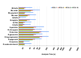
(b) Scalability RTA results.

Figure 5. Scalability results (log scale).

By looking at the figures, it can be seen that RTA outperformed PTA in most experiments and performed especially well in scenarios with a reduced number of threads. For example, the analysis time of Spring Petclinic using only a single thread was reduced by 76 %.

Conversely, as the number of threads increases, the difference is reduced in most benchmarks. It suggests that the current implementation of RTA might contain some scalability bottlenecks. While the implementation of PTA is production-ready and has been optimized for many years, our implementation of RTA is still a research prototype. Therefore, the existence of such scalability bottlenecks is not surprising and suggests that even better results could be achieved if more time is invested into profiling and optimization of the analysis.

4.6. Runtime Performance

Since our implementation of RTA is meant for the development mode and not for production deployments, we focused mainly on the build-time characteristics. In spite of that, we have also collected runtime data for Renaissance and Dacapo to provide a more complete picture. For space reasons, we provide only aggregated statistics. We observed that the time to execute a standard workload for the benchmarks was increased on average by 10 % across all benchmarks, 11 % for Reinaissance, and 8 % for Dacapo. The biggest increase was 26 % for the Renaissance future-genetic benchmark.

Even though such an increase is non-negligible, as already said, RTA is meant to be used for development and testing where such a performance decrease is justified by the reduced build time. If runtime performance is an important criterion, PTA should be considered instead.

4.7. Incrementality

We have implemented the approach described in Section 3.7 and noted that more than 60 % of summaries can be reused for Spring Petclinic, one of the biggest benchmarks, because they satisfy the necessary requirements. Unfortunately, no real benefits were visible when reusing them. It turned out that even though 60 % of the methods did not have to be parsed, parsing these methods only constituted about 33 % of the overall parse time. The methods that would benefit from incrementality the most in our benchmarks are unfortunately the same methods that contain non-trivial embedded constants. As we discussed in Section 3.7, both of these limitations are only implementation specific. They are not inherent to the proposed algorithm and as it turned out that they are blocking the benefits.

5. Related Work

In (Sundaresan et al., 2000; Bacon and Sweeney, 1996), the authors described multiple different approaches (including RTA) on how to construct the application call graph, which is a necessary step for computing reachable program elements. Our approach is an extension of RTA, which is designed to be parallel, incremental, and also provides support for heap snapshotting, a feature necessary for enabling class initialization at build time. In (Sundaresan et al., 2000), the authors also experimented with Variable-Type Analysis, which seems to be similar to the points-to analysis used in GraalVM Native Image. Both works provided only a simple textual description of rapid type analysis without any pseudocode. On the contrary, we provide pseudocode and detailed description for all key components.

Tip and Palsberg gave an overview of various propagation-based call-graph construction algorithms, again including RTA, in (Tip and Palsberg, 2000). Using the terminology from their article, the points-to analysis in Native Image could be classified as 0-CFA. The authors also introduced four new algorithms CTA, FTA, MTA, and XTA that lie between RTA and 0-CFA in the design space. Based on the experimental evaluation, they concluded that their new algorithms, while in theory more powerful than RTA, have only a minor effect with regards to the number of reachable elements (up to less 3 % reachable methods), while being up to 8.3 times slower than RTA. On the other hand, the amount of call graph edges and uniquely resolved polymorphic call sites can be reduced by up to 29 % and 26.3 %, respectively. Since the goal of our research was to reduce the analysis time, and performance is not a priority in development builds, RTA seems to fit our use case best.

In (Titzer, 2006), B. Titzer proposed the Reachable Method Analysis, which is similar to our core algorithm presented in Algorithm 1. Our contributions on top of his analysis are using method summaries, incremental approach, and experimental evaluation of PTA and RTA in the context of Native Image.

Even though the analysis implemented in GraalVM Native Image is context-insensitive and contains several optimizations which aim to increase scalability by sacrificing precision (Wimmer et al., 2019), the analysis can still take minutes for bigger applications. Our version of RTA can reduce the analysis time by up to 64 %.

Grech et al. used heap snapshots to improve the performance and precision of whole program pointer analysis (Grech et al., 2018). However, their analysis is intentionally incomplete; It might miss some reachable program elements. Unfortunately, this is unacceptable for Native Image because if a method that was not marked reachable by static analysis is executed at runtime, it is a fatal error.

There are several tools that compile JVM-based languages into native binaries. Kotlin Native (kot, 2022) and Scala Native (sca, 2022) are two examples of such. However, both of them support only a specific language. We support any language that can be compiled into JVM bytecode. Also, the analysis they use to determine reachable elements is not clearly specified.

The OVM Real-time Java VM (Armbruster et al., 2007) AOT compiles Java applications into executable images. The OVM compiler uses an analysis method called Reaching Types Analysis to detect what parts of code are reachable, but the authors do not specify any details about the analysis in the paper.

6. Conclusions

In this paper, we have introduced a new variant of rapid type analysis (RTA), which is parallel, incremental, and supports heap snapshotting. The incrementality is enabled by the use of method summaries, which can be serialized and reused between multiple builds. We have described the analysis by providing pseudocode for all key components.

The analysis was implemented and evaluated in the context of GraalVM Native Image. RTA was then compared against the poins-to analysis currently used in GraalVM Native Image. We used the Java benchmark suites Renaissance and Dacapo along with example applications for the mainstream Java microservice frameworks Spring, Micronaut, and Quarkus. The experimental evaluation showed, e.g., that RTA can reduce the analysis time of the Spring Petclinic demo application by 64 % at the cost of increasing the image size by 15 %.

We also experimented with the scalability of both our RTA and points-to analysis wrt. the number of processor cores showing that, for a reduced number of threads such as 1 or 4, the savings in the analysis time can be even greater, making RTA a good choice for constrained environments such as GitHub Actions or similar CI pipelines.

In the future, we plan to lift the restrictions currently imposed on which method summaries can be reused. On top of that, we plan to extend the incremental analysis by a concept of summary aggregation whose goal is to merge summaries of directly connected methods. Fewer but larger summaries should be beneficial when method summaries are serialized and reused, boosting the effect of incrementality.

Appendix A Detailed Results

Results for all our benchmarks are presented in Table 5.

Table 5. Detailed statistics of the evaluated benchmarks.

		Reachable Methods		Analysis Time [s]		Total time [s]		Binary size [MB]
Suite	Benchmark	PTA	RTA	PTA	RTA	PTA	RTA	PTA	RTA
Console	helloworld	18	+17%	14	+21%	36	+17%	13	+23%
Dacapo	avrora	24	+25%	12	-8%	51	+6%	23	+30%
	batik	52	+12%	25	-24%	80	-2%	61	+18%
	fop	94	+4%	46	-30%	128	-10%	105	+11%
	h2	40	+8%	20	-25%	69	-4%	52	+10%
	jython	71	+8%	55	-35%	140	-26%	134	+9%
	luindex	26	+23%	13	-8%	54	+7%	32	+25%
	lusearch	24	+25%	12	-8%	49	+6%	29	+28%
	pmd	62	+5%	29	-31%	90	-7%	72	+10%
	sunflow	52	+12%	27	-26%	88	-2%	46	+24%
	xalan	48	+6%	24	-29%	76	-5%	48	+15%
Microservices	micronaut-helloworld-wrk	74	+4%	34	-32%	88	-9%	45	+18%
	mushop:order	168	+2%	102	-59%	209	-30%	104	+13%
	mushop:payment	82	+4%	36	-33%	91	-10%	50	+14%
	mushop:user	115	+3%	57	-44%	135	-18%	76	+13%
	petclinic-wrk	207	+4%	159	-64%	297	-35%	144	+15%
	quarkus-helloworld-wrk	52	+6%	18	-22%	69	-3%	50	+4%
	quarkus:registry	111	+5%	49	-39%	126	-16%	69	+19%
	spring-helloworld-wrk	67	+4%	30	-33%	87	-10%	47	+13%
	tika-wrk	82	+6%	29	-28%	117	-6%	88	+6%
Renaissance	akka-uct	35	+17%	17	0%	49	+2%	22	+23%
	als	317	+6%	1558	-94%	X	X	X	X
	chi-square	173	+8%	129	-60%	260	-30%	100	+17%
	dec-tree	324	+6%	2009	-95%	X	X	X	X
	dotty	83	+10%	37	-16%	98	-4%	51	+16%
	finagle-chirper	89	+8%	45	-29%	105	-12%	51	+16%
	finagle-http	88	+7%	48	-33%	111	-14%	50	+18%
	fj-kmeans	26	+23%	11	0%	35	+6%	18	+22%
	future-genetic	27	+22%	15	0%	44	+5%	19	+21%
	gauss-mix	189	+8%	146	-61%	286	-32%	107	+17%
	log-regression	334	+7%	2215	-95%	X	X	X	X
	mnemonics	26	+23%	15	0%	43	+2%	18	+22%
	movie-lens	177	+8%	109	-59%	222	-29%	106	+15%
	naive-bayes	320	+6%	1277	-92%	X	X	X	X
	page-rank	171	+8%	129	-60%	258	-31%	119	+13%
	par-mnemonics	27	+19%	15	0%	43	+5%	19	+16%
	philosophers	28	+18%	19	+16%	48	+10%	19	+16%
	reactors	30	+13%	19	+16%	47	+11%	19	+21%
	rx-scrabble	27	+22%	14	0%	42	+2%	27	+15%
	scala-doku	27	+22%	11	0%	35	+6%	19	+21%
	scala-kmeans	26	+23%	14	0%	41	+2%	18	+22%
	scala-stm-bench7	30	+20%	19	+26%	49	+14%	19	+21%
	scrabble	27	+19%	14	0%	41	+5%	26	+19%

Appendix B Detailed Reachable Program Elements

Reachable program elements (types, methods, and fields) computed by points-to analysis and our RTA for the benchmarks presented in Section 4 are presented in detail in Table 6. As with the previous tables, the number of reachable program elements has been divided by 1,000 and rounded before comparison. By inspecting the table, it can be seen that these three metrics are correlated. Benchmarks with more reachable methods have also more reachable types and fields and vice versa.

Table 6. Reachable program elements (in thousands).

		Reachable Types			Reachable Methods			Reachable Fields
Suite	Benchmark	PTA	RTA	Diff [%]	PTA	RTA	Diff [%]	PTA	RTA	Diff [%]
Console	helloworld	4	4	0%	18	21	+17%	4	5	+25%
Dacapo	avrora	5	6	+20%	24	30	+25%	7	8	+14%
	batik	9	10	+11%	52	58	+12%	18	20	+11%
	fop	15	16	+7%	94	98	+4%	32	32	0%
	h2	7	7	0%	40	43	+8%	11	12	+9%
	jython	10	11	+10%	71	77	+8%	18	19	+6%
	luindex	5	6	+20%	26	32	+23%	8	9	+12%
	lusearch	4	6	+50%	24	30	+25%	7	8	+14%
	pmd	10	11	+10%	62	65	+5%	19	20	+5%
	sunflow	9	10	+11%	52	58	+12%	18	20	+11%
	xalan	8	8	0%	48	51	+6%	15	16	+7%
Microservices	micronaut-helloworld-wrk	13	14	+8%	74	77	+4%	19	19	0%
	mushop:order	29	30	+3%	168	172	+2%	48	49	+2%
	mushop:payment	15	16	+7%	82	85	+4%	21	21	0%
	mushop:user	20	21	+5%	115	118	+3%	31	31	0%
	petclinic-wrk	39	40	+3%	207	216	+4%	65	66	+2%
	quarkus-helloworld-wrk	11	11	0%	52	55	+6%	15	16	+7%
	quarkus:registry	20	21	+5%	111	117	+5%	28	29	+4%
	spring-helloworld-wrk	12	13	+8%	67	70	+4%	19	19	0%
	tika-wrk	16	16	0%	82	87	+6%	27	28	+4%
Renaissance	akka-uct	7	7	0%	35	41	+17%	8	9	+12%
	als	57	58	+2%	317	337	+6%	85	86	+1%
	chi-square	30	31	+3%	173	186	+8%	51	51	0%
	dec-tree	58	59	+2%	324	344	+6%	87	88	+1%
	dotty	15	16	+7%	83	91	+10%	25	26	+4%
	finagle-chirper	16	17	+6%	89	96	+8%	22	23	+5%
	finagle-http	16	17	+6%	88	94	+7%	22	22	0%
	fj-kmeans	5	6	+20%	26	32	+23%	6	7	+17%
	future-genetic	5	6	+20%	27	33	+22%	6	7	+17%
	gauss-mix	32	34	+6%	189	204	+8%	54	54	0%
	log-regression	59	60	+2%	334	357	+7%	88	89	+1%
	mnemonics	5	6	+20%	26	32	+23%	6	7	+17%
	movie-lens	31	32	+3%	177	191	+8%	51	52	+2%
	naive-bayes	57	59	+4%	320	339	+6%	86	87	+1%
	page-rank	30	31	+3%	171	184	+8%	49	50	+2%
	par-mnemonics	5	6	+20%	27	32	+19%	6	7	+17%
	philosophers	5	6	+20%	28	33	+18%	6	7	+17%
	reactors	6	6	0%	30	34	+13%	7	7	0%
	rx-scrabble	5	6	+20%	27	33	+22%	6	7	+17%
	scala-doku	5	6	+20%	27	33	+22%	6	7	+17%
	scala-kmeans	5	6	+20%	26	32	+23%	6	7	+17%
	scala-stm-bench7	6	6	0%	30	36	+20%	7	7	0%
	scrabble	5	6	+20%	27	32	+19%	6	7	+17%

Appendix C Detailed Scalability Results

Detailed scalability results are presented in Figure 6 and Figure 7.

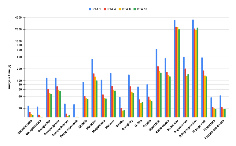
Figure 6. Scalability PTA results (log scale).

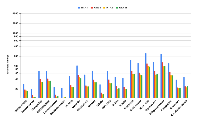
Figure 7. Scalability RTA results (log scale).