Schwinger boson symmetric spin liquids of Shastry-Sutherland model

Abstract

Motivated by recent experimental and numerical evidences of deconfined quantum critical point and quantum spin-liquid states in spin-$1/2$ Heisenberg model on Shastry-Sutherland lattice, we studied possible symmetric spin liquid states and their proximate ordered states under Schwinger boson formalism. We found a symmetric gapped $Z_{2}$ spin-liquid state for intermediate model parameter $0.66<J_{1}/J_{2}<0.71$ under mean-field approximation. The Schwinger boson mean-field picture is partially supported by exact-diagonalization and self-consistent spin wave theory results.

I Introduction

Recently the quasi-two-dimensional materials $S=1/2$ quantum magnets $\rm SrCu_{2}(BO_{3})_{2}$[1, 2, 3, 4] attracted a lot of research interest, as they are one of the most promising realizations of deconfined quantum critical points (DQCP)[5, 6, 7, 8] or spin-liquid states[9]. The in-plane antiferromagnetic (AFM) Heisenberg interactions between the copper atoms of $\rm SrCu_{2}(BO_{3})_{2}$ makes it a potential realization of the Shastry-Sutherland model[10] shown in Fig. 1 (a). Depending on the values of the nearest neighbor couplings $J_{1}$ and the second neighbor couplings $J_{2}$, the Shastry-Sutherland model can host a dimer valence bond solid ground state in the $J_{2}/J_{1}\gg 1$ limit, or a Néel state in the $J_{1}/J_{2}\gg 1$ limit. The issue is the intermediate phase [11, 12, 13, 14] between the Néel phase and dimer-singlet (DS) phase [also called orthogonal dimer (OD) phase in some literature]. There are a variety of prediction of the intermediate phase by difference theories and numerics: a direct transition from dimer-singlet phase to Néel phase[15, 16], a helical order[17, 18], columnar dimers[19], or plaquette-singlet[12, 16, 18] intermediate phase. Recently there are experimental[2, 3, 4] and numerical[20, 14, 21, 22, 23] evidences of the existence of the plaquette-singlet (PS) phase [also called plaquette singlet solid (PSS) or plaquette valence bond solid (PVBS) in some literature]. The phase transition between the Néel and plaquette-singlet phase may be described by a DQCP with emergent $O(4)$ symmetry[13, 20] and deconfined spinon excitations. And evidences of a proximate DQCP were found on the boundary of plaquette-singlet phase and Néel AFM phase in a NMR study of $\rm SrCu_{2}(BO_{3})_{2}$ under external magnetic field[1].

Some recent numerical studies including density-matrix renormalization group (DMRG)[24], exact diagonalization(ED)[25], and pseudofermion functional renormalization group[26] also suggest the existence of a spin liquid phase in a narrow range of coupling parameter $J_{1}/J_{2}$ between the PS phase and Néel phase without magnetic field. This intriguing possibility has not been thoroughly studied theoretically, especially using the traditional slave particle language for spin liquids[27]. With this motivation we study the possible symmetric spin-liquid states and their proximate ordered states on Shastry-Sutherland lattice under Schwinger boson formalism[28] in this paper. The goal of our work is not to accurately determine the phase diagram of the Shastry-Sutherland model, but to explore the possibilities of quantum spin liquids compatible with this lattice, which might be realized in related models and materials.

In this paper, we focus on the Schwinger boson[29] description of quantum spin liquids. This formalism and its large-$N$ generalization[30] are convenient to describe the transition between gapped $Z_{2}$ spin-liquid phases and magnetic ordered phases[28], and have been successful in the studies of several quantum magnets[31]. By projective symmetry group (PSG)[32, 33], we find 6 possible algebraic $Z_{2}$ PSG solutions and 4 gauge inequivalent ansatz. Comparing the mean-field energies of these ansatz, we find a symmetric gapped $Z_{2}$ spin liquid for the intermediate model parameter $0.66<J_{1}/J_{2}<0.71$ under mean-field approximation. A dimer-singlet phase forms in $J_{1}/J_{2}<0.66$ while a Néel AFM state forms in $J_{1}/J_{2}>0.71$, where the Schwinger boson condensation happens. To further investigate the PS state, we also study ansatz with PS order, and find that these PS ansatz have higher ground state energy compared with the symmetric spin liquids in the mean-field level.

We also study the spin correlations of ground state wave function and structure factor of the spin-liquid states and Néel state by the Schwinger boson mean-field theory(SBMFT), and compare them with the results of exact-diagonalization and spin-wave theory. We find that the spin correlations in SBMFT have similar behavior compared with the result of the exact diagonalization method. The structure factor in the Néel phase can also be calculated by the spin wave theory. However, the linear spin wave theory breaks down near $J_{1}/J_{2}\sim 1$, which is far from the Néel phase boundary. To investigate the Néel phase in $J_{1}/J_{2}<1$ region, we use a self-consistent spin wave theory, which pushes the Néel phase boundary down to $J_{1}/J_{2}\approx 0.65$. With the self-consistent spin wave theory, we get qualitatively consistent dynamical spin correlations with Schwinger boson mean-field theory.

This paper is organized as follows. In Sec. II, We introduce the Shastry-Sutherland model and Schwinger boson mean-field theory, present the mean-field phase diagram with a gapped $Z_{2}$ spin liquid state in the intermediate parameter $0.66<J_{1}/J_{2}<0.71$. In Sec. III, we compare the structure factors for the spin liquid and Néel states by SBMFT and self-consistent spin wave theory, and compare some of the ground state properties by SBMFT and exact diagonalization. Section IV contains further discussion and a summary of results. The technical and numerical details are presented in the Supplemental Material.

II Schwinger boson symmetric spin liquids

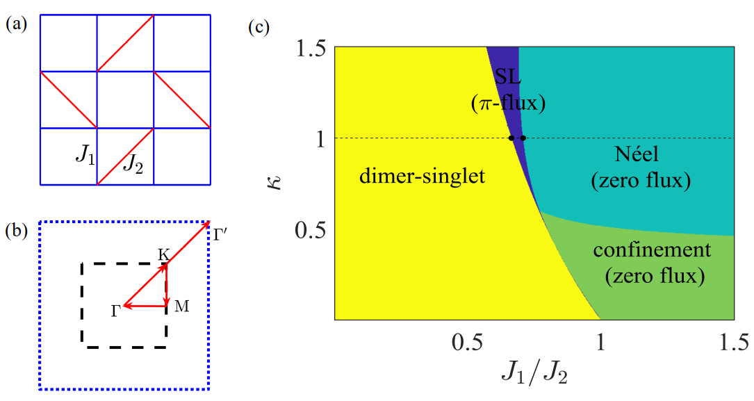
Figure 1: (a) is the Shastry-Sutherland lattice. The Heisenberg couplings in blue and red bonds are $J_{1}$ and $J_{2}$ respectively. The black dashed line in (b) is the first Brillouin zone of Shastry-Sutherland lattice, and the blue dotted line is the first Brillouin zone of square lattice without $J_{2}$ bonds. The red arrows are the plot paths ($\mathrm{K}\rightarrow\mathrm{M}\rightarrow\mathrm{\Gamma}\rightarrow\mathrm{K}\rightarrow\mathrm{\Gamma^{\prime}}$) in this paper. (c) is the phase diagram of Schwinger boson mean-field theory for Shastry-Sutherland model. The phase boundaries at physical condition $\kappa=1$ are $J_{1}/J_{2}=0.66$ and $J_{1}/J_{2}=0.71$. In the mean-field level, the phase transition from DS to SL is continuous while the phase transition from SL to Néel is first order.

The Shastry-Sutherland model Hamiltonian is

$$H=J_{1}\sum_{\langle ij\rangle}\mathbf{S}_{i}\cdot\mathbf{S}_{j}+J_{2}\sum_{\langle\langle ij\rangle\rangle^{\prime}}\mathbf{S}_{i}\cdot\mathbf{S}_{j},$$ (1)

where $\mathbf{S}_{i}$ are $S=1/2$ spin operators and $\langle ij\rangle$ are the nearest-neighbor[blue in Fig. 1(a)] bonds, while $\langle\langle ij\rangle\rangle^{\prime}$ are some of the next-nearest-neighbor[red in Fig. 1(a)] bonds. Here we study this Hamiltonian by the Schwinger boson mean-field theory. The spin operator is expressed by the Schwinger bosons as

$$\bm{S}_{i}=\frac{1}{2}\sum_{\alpha,\beta=\uparrow,\downarrow}b_{i\alpha}^{\dagger}\bm{\sigma}_{\alpha\beta}b_{i\beta},$$ (2)

with the constraints at every site

$$\sum_{\sigma}b_{i\sigma}^{\dagger}b_{i\sigma}=\kappa=2S,$$ (3)

for a spin system with spin $S$. For the convenience of analysis, $\kappa$ is usually regarded as a continuous parameter. Using the Schwinger boson representation, the Heisenberg interaction can be rewritten as

$$\bm{S}_{i}\cdot\bm{S}_{j}=:\hat{B}_{ij}^{\dagger}\hat{B}_{ij}:-\hat{A}_{ij}^{\dagger}\hat{A}_{ij}$$ (4)

where $::$ is normal ordering and boson pairing operator $\hat{A}$ and hopping operator $\hat{B}$ are defined as

$$\hat{B}_{ij} = \frac{1}{2}\sum_{\sigma}b_{i\sigma}^{\dagger}b_{j\sigma},$$ (5)

$$\hat{A}_{ij} = \frac{1}{2}\sum_{\sigma,\sigma^{\prime}}\epsilon_{\sigma\sigma^{\prime}}b_{i\sigma}b_{j\sigma^{\prime}}.$$ (6)

After decoupling the quartic terms by the Hubbard-Stratonovich transformation, we get the mean-field Hamiltonian:

$$H_{\mathrm{MF}} = \sum_{ij}J_{ij}\left(-A_{ij}^{*}\hat{A}_{ij}+B_{ij}^{*}\hat{B}_{ij}+\text{ H.c. }\right)$$ (7)

$$+ \sum_{ij}J_{ij}\left(\left|A_{ij}\right|^{2}-\left|B_{ij}\right|^{2}\right)-\mu_{i}\sum_{i}\left(\hat{n}_{i}-\kappa\right),$$

where the complex numbers $A_{ij}=\langle\hat{A}_{ij}\rangle=-A_{ji}$ and $B_{ij}=\langle\hat{B}_{ij}\rangle=B_{ji}^{*}$ are the mean-field ansatz. $\mu_{i}$ are the real Lagrangian multipliers to enforce the constraints of Eq. (3), which are usually site independent, namely $\mu_{i}=\mu$. This mean-field description has emergent $U(1)$ gauge redundancy, namely that the following $U(1)$ gauge transformation, $b_{j\sigma}\to e^{i\phi(j)}b_{j\sigma}$, $A_{jk}\to e^{i[\phi(j)+\phi(k)]}A_{jk}$, and $B_{jk}\to e^{i[-\phi(j)+\phi(k)]}B_{jk}$, will not change the physical spin states. Therefore the mean-field solutions should be classified by projective symmetry group(PSG)[32, 33]. With the help of the PSG of Schwinger boson, we find 6 PSG solutions and 4 gauge inequivalent ansatz which are named as $(\pi,\pi)$, $(0,\pi)$, $(\pi,0)$, and $(0,0)$-flux states according to their gauge flux distribution. The gauge invariant “flux” values $\Phi_{1}$ and $\Phi_{2}$ in the empty squares and $J_{2}$ squares respectively, are defined as the complex phase of the product of nearest-neighbor boson pairing ansatz $A_{ij}(-A_{jk}^{*})A_{kl}(-A_{li}^{*})$ around a plaquette[34]. Due to time reversal symmetry $\Phi_{1}$ and $\Phi_{2}$ can only be $0$ or $\pi$, and the four different combinations of $(\Phi_{1},\Phi_{2})$ corresponds to the 4 gauge inequivalent ansatz solved by PSG. The $(\pi,\pi)$ and $(0,0)$-flux states are called $\pi$-flux and zero-flux hereafter. The details of the PSG solutions and ansatz are shown in Supplemental Material.

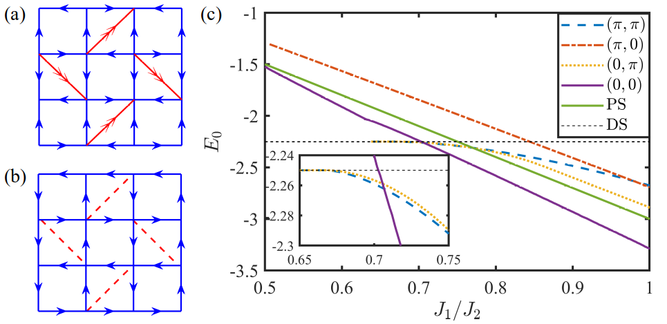
Figure 2: (a) and (b) are the ansatz $A_{ij}$ of the zero-flux and $\pi$-flux states respectively. An arrow from site $i$ to $j$ means $A_{ij}>0$ and $A_{ij}$ in dashed lines are zero. The different arrows represent different amplitudes of $A_{ij}$. (c) is the ground state energies of the 4 gauge inequivalent symmetric spin liquid ansatz and two valence bound solid (DS and PS) states for $\kappa=1$. The inset in (c) is the details in $0.65<J_{1}/J_{2}<0.75$. It shows that only the DS state and $(\pi,\pi)$-flux and $(0,0)$-flux SL states appear as mean-field ground states for $\kappa=1$.

Comparing the mean-field ground state energies of the 4 gauge inequivalent symmetric ansatz with the change of $J_{1}/J_{2}$ and $\kappa$, we get a mean-field phase diagram of the Heisenberg model in Shastry-Sutherland lattice, which is shown in Fig. 1 (c). We find only two ansatz with zero or $\pi$-flux in each plaquettes as mean-field ground states under physical condition ($\kappa=1$). The ansatz configuration of these two state are shown in Fig. 2 (a) and (b).

The zero-flux state is the mean-field ground state for large $J_{1}$ ($J_{1}/J_{2}>0.71$ at $\kappa=1$). The emergent gauge field for the zero-flux state is a staggered $U(1)$ gauge field, and the spinons are either confined (possibly forming valence bond solid) when $\kappa$ is small[35] or condensed when $\kappa$ is large. For physical $\kappa=1$ the spinons of zero-flux state condense and form the Néel AFM order. The zero-flux Schwinger boson state and related phases has been discussed before in the context of square lattice antiferromagnets[30].

The $\pi$-flux state is the mean-field ground state for small $J_{1}$ ($J_{1}/J_{2}<0.71$ at $\kappa=1$). For intermediate $J_{1}$ ($0.66<J_{1}/J_{2}<0.71$ at $\kappa=1$) this state has $Z_{2}$ gauge field. For physical $\kappa=1$ the spinons of this state are gapped and form a gapped $Z_{2}$ spin liquid. For very high $\kappa$ ($\kappa\gtrsim 2.5$ for $J_{1}/J_{2}\sim 0.7$) the bosons will condense and likely form a 4-sublattice antiferromagnetic order similar to the $\pi$-flux Schwinger boson state of square lattice antiferromagnets[36].

In the lowest $J_{1}$ region ($J_{1}/J_{2}<0.66$ at $\kappa=1$) the $\pi$-flux state reduces to the confined dimer-singlet state with only next-nearest-neighbor boson pairing $A_{2}\neq 0$.

Therefore, there are three distinct phases with the change of $J_{1}/J_{2}$ for physical $\kappa=1$ under mean-field approximation: dimer-singlet phase for $J_{1}/J_{2}<0.66$, $\pi$-flux $Z_{2}$ spin liquid state for $0.66<J_{1}/J_{2}<0.71$ and Néel phase for $J_{1}/J_{2}>0.71$. The details of PSG and mean-field solution can be referred to the Supplemental Material.

The dynamic and static structure factors of the $\pi$-flux spin liquid state are also calculated by the Schwinger boson mean field theory and shown in Fig. 3, which may be used as numerical and experimental signatures of this spin liquid state. In particular the dominant short-range spin correlations in this $\pi$-flux SL state is related to a 4-sublattice AFM order (see Supplemental Material).

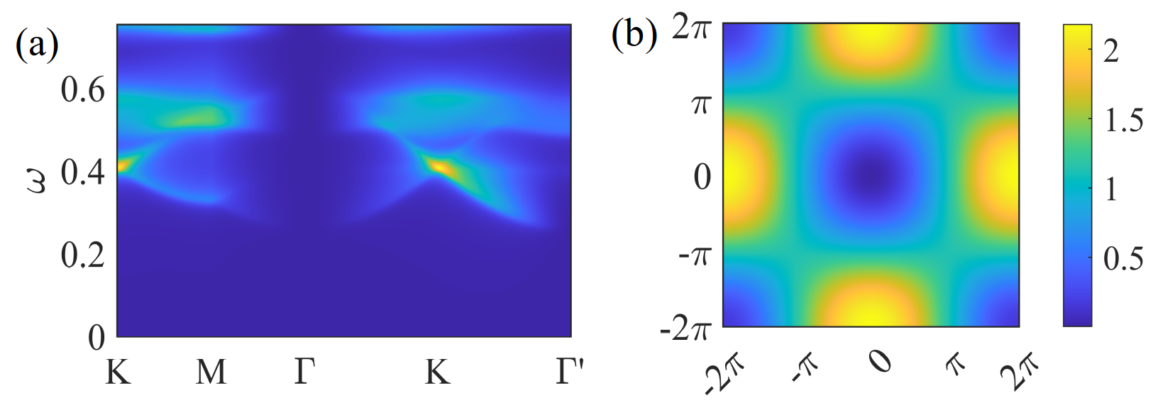
Figure 3: (a) and (b) are the dynamic and static structure factor respectively of the $\pi$-flux $Z_{2}$ spin liquid phase. The model parameters are $J_{1}=0.7$, $J_{2}=1$. Note the plotting range of (b) is the first BZ of the square lattice without $J_{2}$ bonds.

To further investigate the PS phase, we also study mean-field ansatz with plaquette-singlet order. There are two kinds of plaquette-singlet states for the two kinds of plaquette in Shastry-Sutherland lattice. Only the mean field energy of plaquette-singlet state in the “empty” square is plotted in Fig. 2 (c), because it has lower ground state energy. The details of the plaquette-singlet state can be referred to Supplemental Material. We find that the ground state energy of this state is always higher comparing with the minimum energy of $\pi$ and zero-flux SL states with the change of parameter $J_{1}/J_{2}$, which is shown in Fig. 2 (c). However, the energy differences are small near the intermediate region of parameter $J_{1}/J_{2}$ with $\pi$-flux SL ground state. Therefore, the PS state may emerge after considering the gauge fluctuations and projecting the mean-field wave function by Gutzwiller projection, which is beyond the scope of the current work. Because of the absence of the PS state in the mean-field level, the possible DQCP[13, 20] cannot be studied by the Schwinger boson mean field theory.

III Comparison to self-consistent spin wave theory and ED

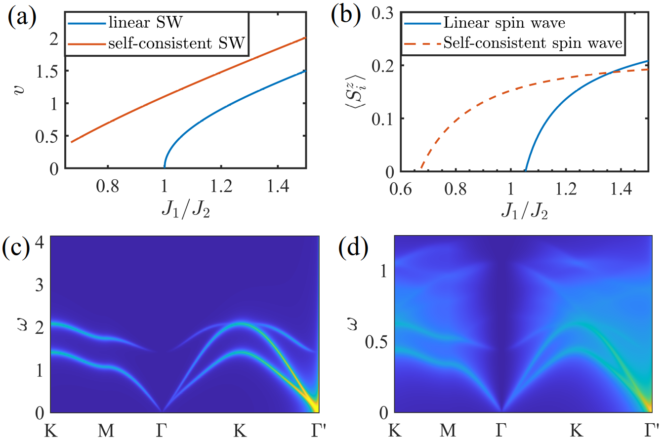
Figure 4: (a) is the magnon velocity near the Goldstone mode calculated by linear spin wave and self-consistent spin wave theory (see Supplemental Material). The magnon velocity of linear spin wave vanishes at $J_{1}/J_{2}=1$, where the magnon dispersion become $\propto k^{2}$ and linear spin wave theory breaks down. (b) is the Néel order parameter computed by self-consistent spin wave theory and linear spin wave theory, which vanishes at $J_{1}/J_{2}\approx 0.65$ and $J_{1}/J_{2}\approx 1.05$ respectively. (c) and (d) are the dynamic structure factor calculated by self-consistent spin wave theory and Schwinger boson mean-field theory in Néel phase. The parameters are $J_{1}=0.9$, $J_{2}=1$.

The Néel phase can also be studied by the spin wave theory. However, as shown in Fig. 4 (a) and (b), the linear spin wave theory breaks down at $J_{1}/J_{2}=1$ because the spin wave dispersion become $\epsilon_{k}\propto k^{2}$ under linear spin wave at $J_{1}/J_{2}=1$, and the magnetic order parameter for spin-1/2 model vanishes at $J_{1}/J_{2}=1.05$, which is much larger than the Néel phase boundary by other theories and numerics. The details of the spin wave dispersion can be referred to Supplemental Material. Near the Néel phase boundary, the magnon interactions play important roles and need to be considered. However, the conventional nonlinear spin wave theory by $1/S$ expansion also breaks down near $J_{1}/J_{2}=1$ because the interaction correction depends on the linear spin wave Hamiltonian. Therefore, we use the self-consistent spin wave theory[37, 38] to incorporate the effects of magnon interactions. The idea of the self-consistent spin wave theory is to decouple the quartic terms of Holstein-Primakoff bosons into all possible quadratic terms, and compute these corrections to linear spin wave Hamiltonian self-consistently. The details of the self-consistent spin wave theory are given in the Supplemental Material. The magnetic order parameter vanishes at $J_{1}/J_{2}\approx 0.65$ by self-consistent spin wave theory as shown in Fig. 4 (b), which yields more accurate Néel phase boundary.

The dynamic structure factors in the Néel phase are calculated to compare the self-consistent spin wave theory and the Schwinger boson mean-field theory. Fig. 4 (c) and (d) are the dynamic structure factors at $J_{1}/J_{2}$=0.9 calculated by these two theories. In the Néel phase, the Schwinger boson condenses and yields sharp magnon peaks in the dynamic structure factor, while the non-condensing spinons contribute to the continuum. Although the magnon interaction is considered in the self-consistent spin wave theory, the magnon damping channel is not included. Therefore, the magnon peaks are always sharp and there is no continuum in the dynamic structure factor calculated by self-consistent spin wave theory. The dynamic structure factor calculated by self-consistent spin wave theory is more consistent with the schwinger boson mean field theory than the linear spin wave theory. We note that the energy scales of dynamic structure factors are different in the Schwinger boson mean-field theory and spin wave theory, and they should become identical in the large $S$ limit.

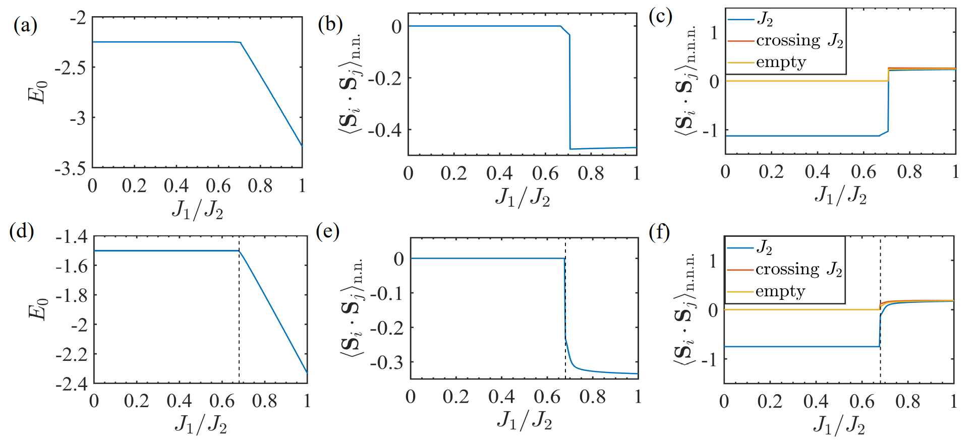
Figure 5: (a), (c), (e) and (b), (d), (f) are observables calculated by Schwinger boson mean-field theory and 32-site exact diagonalization respectively. (a) and (b) are the ground state energy per unit cell. (c) and (d) are the nearest-neighbor (n.n.) spin correlation. (e) and (f) are the next-nearest-neighbor (n.n.n.) spin correlation. The Shastry-Sutherland lattice has three inequivalent n.n.n. bonds, which are $J_{2}$ bond, bond crossing $J_{2}$ bond, and empty bond. The dashed lines in (b), (d) and (f) are $J_{1}/J_{2}=0.68$. The discontinuity of spin correlation functions and slope of ground state energies at $J_{1}/J_{2}=0.71$ in(a)(c)(e) indicates that the transition from $\pi$-flux spin liquid to Néel order is first order under mean-field approximation, while the transition from DS to $\pi$-flux spin liquid at $J_{1}/J_{2}=0.66$ seems continuous. Note that in (e) $\langle\boldsymbol{S}_{i}\cdot\boldsymbol{S}_{j}\rangle_{\text{n.n.n}}$ is less than $-3/4$ (the minimal possible value for spin-$1/2$) in some parameter range, this is due to the spin size(boson number) fluctuation in the mean-field approximation[33].

We also compare the ground state properties computed by SBMFT and exact diagonalization. The results are shown in Fig. 5. The ground state from 32-site exact diagonalization is the exact dimer-single state for $J_{1}/J_{2}<0.68$, which is consistent with previous exact diagonalization studies[11, 39] and very close to the SBMFT phase boundary $J_{1}/J_{2}\sim 0.66$ for DS phase. The near-neighbor and next-nearest-neighbor spin correlations also show similar behavior in SBMFT and exact diagonalization.

IV Discussion and conclusion

We studied the Shastry-Sutherland model by the Schwinger boson mean field theory. Using the projective symmetry group method, we find two kinds of possible symmetric ansatz. Comparing the energy of the two ansatz with the change of $J_{1}/J_{2}$ and $\kappa$, we get the Schwinger boson mean-field phase diagram of Shastry-Sutherland model. We find a $\pi$-flux gapped $Z_{2}$ spin liquid state for the intermediate parameter $0.66<J_{1}/J_{2}<0.71$ between the dimer-singlet phase and the Néel AFM phase. This $\pi$-flux spin liquid state is continuously connected to the DS phase, but has a first-order transition to the Néel AFM phase upon increasing $J_{1}/J_{2}$, which can be seen from the discontinuity of spin correlation functions and slope of ground state energies in the Schwinger boson mean-field results in Fig. 5. The continuous transition between the spin liquid and DS phases is an example of the confinement transition of Ising gauge field[40], which can be described by the condensation of gauge flux excitations (“visons”) and should be dual to an 3D Ising transition. The short-range spin correlations in the $\pi$-flux state is closely related to a 4-sublattice AFM order instead of Néel AFM order. We expect that ring-exchange coupling with opposite sign to that derived from the Hubbard model would further stabilize this $\pi$-flux spin liquid state[33].

To investigate the possibility of plaquette-singlet state[12, 16, 18, 20, 14, 21, 22], we studied PS ordered ansatz which break the glide symmetry. We found that the ground state energy of these PS ordered ansatz are higher compared with the symmetric spin liquid ansatz under mean-field approximation. Therefore, the PS phase does not exist in our mean-field phase diagram. However the energy difference between the PS phase and spin liquids are small in the spin liquid phase. So it is possible that the PS phase may emerge after considering gauge fluctuations and Gutzwiller projection of mean-field wave functions, which we leave for future studies.

To further investigate the Néel AFM phase, we used a self-consistent spin wave theory because the linear spin wave theory breaks down for $J_{1}/J_{2}<1$. The self-consistent spin wave theory renormalizes the magnon dispersion by the magnon interactions, and further stabilizes the magnetic order down to $J_{1}/J_{2}\sim 0.65$. The dynamic structure factor calculated by this theory is more consistent with the results of Schwinger boson mean-field theory except for an overall energy scale.

We have also performed exact diagonalization of the Shastry-Sutherland model with $32$ sites. The results indicate that the phase boundary of dimer-singlet phase is $J_{1}/J_{2}\sim 0.68$, which is roughly consistent with the Schwinger boson mean-field result and previous exact diagonalization studies of larger system sizes[39]. The behavior of spin correlation functions from the exact diagonalization results is similar to those of the Schwinger boson mean-field theory, which provides partial support of our mean-field picture of the Shastry-Sutherland model.

Some previous numerical studies[24, 25, 26] suggest that the spin liquid phase in Shastry-Sutherland model is gapless and possibly described by fermionic spinons with Dirac-cone dispersions similar to the DQCP[20]. This gapless spin liquid phase cannot be captured by our Schwinger boson mean-field theory. However strong interactions between fermionic spinons induced by gapless $U(1)$ gauge field might produce Cooper pairing of spinons, which may open spin gap and reduce the $U(1)$ gauge field to $Z_{2}$. The possible transition from $U(1)$ to $Z_{2}$ spin liquids may be studied in controlled large-$N$ approximation[41]. The resulting gapped $Z_{2}$ fermionic spinon spin liquid is likely a dual description of the Schwinger boson symmetric $Z_{2}$ spin liquids considered here[42], and may be an interesting direction for future theoretical and numerical studies. However it should be noted that the “$\pi$-flux” for Abrikosov fermion hoppings in this $U(1)$ spin liquid[20] is not directly related to the “$\pi$-flux” of boson pairing terms in our Schwinger boson formalism.

V ACKNOWLEDGEMENTS

KL thanks Fang-Yu Xiong, Xue-Mei Wang and Jie-Ran Xue for helpful discussions. FW acknowledges support from National Natural Science Foundation of China (No. 12274004), and National Natural Science Foundation of China (No. 11888101).

Appendix A PSG classification of the symmetric spin liquid on Shastry-Sutherland lattice

The Schwinger boson mean-field theory has a emergent $U(1)$ gauge symmetry. After the local gauge transformation

$$b_{j\sigma} \rightarrow e^{i\phi(j)}b_{j\sigma},$$ (8)

$$A_{ij} \rightarrow e^{i[\phi(i)+\phi(j)]}A_{ij},$$ (9)

$$B_{ij} \rightarrow e^{i[-\phi(i)+\phi(j)]}B_{ij},$$ (10)

the mean-field Hamiltonian is invariant and all physical observables are unchanged, as the wave function is same after projected to physical condition. Because of the existence of emergent gauge symmetry, for different spin liquids with same symmetry, the ansatz are invariant under symmetry transformations followed by gauge transformations, $\hat{b}_{\boldsymbol{r},s}\to\exp[\mathbbm{i}\phi_{g}(g\boldsymbol{r})]\hat{b}_{g\boldsymbol{r},s}$, for space group element $g$. Therefore, the spin-liquid states should be classified by the projective representation of the space group. The ansatz are invariant under operations of projective symmetry group (PSG). Different PSGs characterize different kinds of spin-liquid states with same symmetries.

We set up a Cartesian coordinate system and represent the site coordinate by $(x,y)=x\hat{e}_{x}+y\hat{e}_{y}$ with $x,y\in\mathbb{Z}$. For the discussion convenience, the site coordinate can also be expressed by cell-sublattice index, $(X,Y,s)$, where $X,Y\in\mathbb{Z}$ and $s\in\mathbb{Z}_{4}$ ($s=0,1,2,3$), which means Cartesian $(2X+x_{s},2Y+y_{s})$ with $(x_{0},y_{0})=(0,0)$, $(x_{1},y_{1})=(1,0)$, $(x_{2},y_{2})=(1,1)$, $(x_{3},y_{3})=(0,1)$. The sublattice labeling is shown in Fig. 6. With these two coordinate systems, the nearest-neighbor(n.n.) bonds are $(x,y)-(x+1,y)$ and $(x,y)-(x,y+1)$ while the next-nearest-neighbor(n.n.n.) bonds are $(X,Y,0)-(X,Y-1,2)$ and $(X,Y,1)-(X+1,Y,3)$.

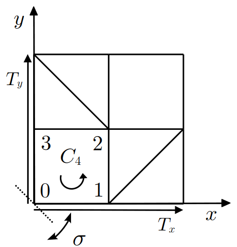
Figure 6: The coordinate system and space group generators $T_{x}$, $T_{y}$, $C_{4}$, $\sigma$ of the Shastry-Sutherland lattice. These generators are translation $T_{x}$ along $\hat{e}_{x}$ by 2 units, translation $T_{y}$ along $\hat{e}_{y}$ by 2 units, a reflection $\sigma$ about $x=-y$ and the $90^{\circ}$ rotation $C_{4}$ around $(1/2,1/2)$.

The space group of the square lattice is generated by translation $T_{x}$ along $\hat{e}_{x}$ by 2 units, translation $T_{y}$ along $\hat{e}_{y}$ by 2 units, a reflection $\sigma$ along $x=-y$ and the $90^{\circ}$ rotation $C_{4}$ around $(1/2,1/2)$, which are also shown in Fig. 6. The action of these generators on the Shastry-Sutherland lattice reads

$$T_{X}^{\vphantom{-1}} : \quad(x,y)\mapsto(x+2,y),\quad(X,Y,s)\mapsto(X+1,Y,s),$$ (11)

$$T_{Y}^{\vphantom{-1}} : \quad(x,y)\mapsto(x,y+2),\quad(X,Y,s)\mapsto(X,Y+1,s),$$ (12)

$$C_{4}^{\vphantom{-1}} : \quad(x,y)\mapsto(-y+1,x),\quad(X,Y,s)\mapsto(-Y,X,(s+1)\mod 4),$$ (13)

$$\sigma^{\vphantom{-1}} : \quad(x,y)\mapsto(-y,-x),\quad(X,Y,s)\mapsto(-Y-y_{s},-X-x_{s},(-s)\mod 4).$$ (14)

These generators have the following commutative relations,

$$T_{X}^{-1}T_{Y}^{\vphantom{-1}}T_{X}^{\vphantom{-1}}T_{Y}^{-1} = \mathbbm{1},$$ (15)

$$T_{Y}^{-1}T_{X}^{-1}C_{4}^{\vphantom{-1}}T_{X}^{\vphantom{-1}}C_{4}^{-1} = \mathbbm{1},$$ (16)

$$T_{X}^{-1}C_{4}^{\vphantom{-1}}T_{Y}^{-1}C_{4}^{-1} = \mathbbm{1},$$ (17)

$$C_{4}^{4} = \mathbbm{1},$$ (18)

$$T_{X}^{-1}\sigma^{\vphantom{-1}}T_{Y}^{-1}\sigma^{-1} = \mathbbm{1},$$ (19)

$$T_{Y}^{-1}\sigma^{\vphantom{-1}}T_{X}^{-1}\sigma^{-1} = \mathbbm{1},$$ (20)

$$\sigma^{2} = \mathbbm{1},$$ (21)

$$T_{X}^{-1}C_{4}^{\vphantom{-1}}\sigma^{\vphantom{-1}}C_{4}^{\vphantom{-1}}\sigma^{-1} = \mathbbm{1}.$$ (22)

With these relations, any sequence of generators (and their inverses) can be rearranged into the form $T_{X}^{X}T_{Y}^{Y}C_{4}^{s}\sigma^{m}$, with $X,Y\in\mathbbm{Z}$, and $s\in\mathbbm{Z}_{4}=\{0,1,2,3\}$ and $m\in\mathbbm{Z}_{2}=\{0,1\}$. Then the multiplication rule of the space group is determined. This is a faithful representation of the space group, namely any space group element can be uniquely represented by this expression. For a space group element, the image of $(0,0,0)$ site is $(X,Y,s)$, then the remaining freedom is a possible mirror reflection. We omit $(\mod 4)$ for sublattice index hereafter.

A.1 solutions of the algebraic PSG

In the following we will solve the algebraic PSGs by using these algebraic constraints on the generators of the Shastry-Sutherland lattice space group. We only consider the condition where the invariant gauge group (IGG) is $Z_{2}$. For a space ground element $g$, the Schwinger boson operators are transformed as

$$\hat{b}_{\boldsymbol{r},s}\to\exp[\mathbbm{i}\phi_{g}(g\boldsymbol{r})]\hat{b}_{g\boldsymbol{r},s}.$$ (23)

For a defining relation $g_{1}g_{2}\cdots g_{k}=\mathbbm{1}$, we have

$$\phi_{g_{1}g_{2}\cdot g_{k}}(g_{1}g_{2}\cdot g_{k}\boldsymbol{r})+\phi_{g_{2}\cdot g_{k}}(g_{2}\cdot g_{k}\boldsymbol{r})+\dots+\phi_{g_{k}}(g_{k}\boldsymbol{r})=(\text{an IGG element})=p\pi,p\in\mathbbm{Z}_{2}.$$ (24)

Note that all these equations about $\phi$s are implicitly modulo $2\pi$.

We consider a gauge transformation $\hat{b}_{\boldsymbol{r},s}=\exp[\mathbbm{i}\phi(\boldsymbol{r})]\hat{b}^{\prime}_{\boldsymbol{r},s}$, then the generators of PSG transformed as

$$\phi^{\prime}_{g}(g\boldsymbol{r})=\phi_{g}(g\boldsymbol{r})+\phi(g\boldsymbol{r})-\phi(\boldsymbol{r}).$$ (25)

With this relation, by choosing $\phi(X,Y,s)$ for all $X\neq 0$, we can make $\phi^{\prime}_{T_{X}^{\vphantom{-1}}}(X,Y,s)=0$ for all $X,Y,s$;
then by choosing $\phi(X=0,Y,s)$, we can make $\phi^{\prime}_{T_{Y}^{\vphantom{-1}}}(X=0,Y,s)=0$ for all $Y,s$. we are still left three gauge freedoms. The first one is the global constant phase,

$$\phi(X,Y,s)_{1}=\phi_{s},$$ (26)

this does not change $\phi_{T_{X}^{\vphantom{-1}}}$ and $\phi_{T_{Y}^{\vphantom{-1}}}$, but will change $\phi_{C_{4}^{\vphantom{-1}}}$ and $\phi_{\sigma^{\vphantom{-1}}}$ as

$$\phi^{\prime}_{C_{4}^{\vphantom{-1}}}(X,Y,s) = \phi_{C_{4}^{\vphantom{-1}}}(X,Y,s)+\phi_{s}-\phi_{s-1},$$ (27)

$$\phi^{\prime}_{\sigma^{\vphantom{-1}}}(X,Y,s) = \phi_{\sigma^{\vphantom{-1}}}(X,Y,s)+\phi_{s}-\phi_{-s}.$$ (28)

The second gauge freedom is

$$\phi(X,Y,s)_{2}=\pi\cdot X,$$ (29)

which also does not change $\phi_{T_{X}^{\vphantom{-1}}}$ and $\phi_{T_{Y}^{\vphantom{-1}}}$ modulo IGG, but will change $\phi_{C_{4}^{\vphantom{-1}}}$ and $\phi_{\sigma^{\vphantom{-1}}}$ as

$$\phi^{\prime}_{C_{4}^{\vphantom{-1}}}(X,Y,s) = \phi_{C_{4}^{\vphantom{-1}}}(X,Y,s)+\pi\cdot(X-Y),$$ (30)

$$\phi^{\prime}_{\sigma^{\vphantom{-1}}}(X,Y,s) = \phi_{\sigma^{\vphantom{-1}}}(X,Y,s)+\pi\cdot(X-Y-x_{-s}).$$ (31)

The third gauge freedom is

$$\phi(X,Y,s)_{3}=\pi\cdot(X+Y),$$ (32)

which does not change $\phi_{T_{X}^{\vphantom{-1}}}$ and $\phi_{T_{Y}^{\vphantom{-1}}}$ and $\phi_{C_{4}^{\vphantom{-1}}}$ modulo IGG, but will change $\phi_{\sigma^{\vphantom{-1}}}$ as

$$\phi^{\prime}_{\sigma^{\vphantom{-1}}}(X,Y,s) = \phi_{\sigma^{\vphantom{-1}}}(X,Y,s)-\pi\cdot(x_{-s}+y_{-s})$$ (33)

$$= \phi_{\sigma^{\vphantom{-1}}}(X,Y,s)+\pi\cdot s.$$

We then consider the relation of the generators of the space group. From the relation of Eq. (15), the algebraic constraint is ($\phi_{T_{X}^{\vphantom{-1}}}$ omitted hereafter),

$$\phi_{T_{Y}^{\vphantom{-1}}}(X+1,Y,s)-\phi_{T_{Y}^{\vphantom{-1}}}(X,Y,s)=p_{1}\pi,$$ (34)

then the solution is

$$\phi_{T_{Y}^{\vphantom{-1}}}(X,Y,s)=p_{1}\pi\cdot X.$$ (35)

The algebraic constraint from relation of Eq. (16) is

$$-\phi_{T_{Y}^{\vphantom{-1}}}(X,Y+1,s)+\phi_{C_{4}^{\vphantom{-1}}}(X+1,Y+1,s)-\phi_{C_{4}^{\vphantom{-1}}}(X,Y,s)=p_{2}\pi,$$ (36)

then we have

$$\phi_{C_{4}^{\vphantom{-1}}}(X+1,Y+1,s)-\phi_{C_{4}^{\vphantom{-1}}}(X,Y,s)=p_{2}\pi+p_{1}\pi\cdot X$$ (37)

From the relation of Eq. (17), we have

$$\phi_{C_{4}^{\vphantom{-1}}}(X+1,Y,s)-\phi_{T_{Y}^{\vphantom{-1}}}(Y,-X,s-1)-\phi_{C_{4}^{\vphantom{-1}}}(X,Y,s)=p_{3}\pi,$$ (38)

which yields

$$\phi_{C_{4}^{\vphantom{-1}}}(X+1,Y,s)-\phi_{C_{4}^{\vphantom{-1}}}(X,Y,s)=p_{3}\pi+p_{1}\pi\cdot Y.$$ (39)

Combining with Eq. (37), the solution is

$$\phi_{C_{4}^{\vphantom{-1}}}(X,Y,s)=\phi_{C_{4}^{\vphantom{-1}}}(X,Y,s)+p_{2}\pi\cdot Y+p_{3}\pi\cdot(X-Y)+p_{1}\pi\cdot[XY-\frac{1}{2}Y(Y+1)]$$ (40)

Note that we can use the gauge freedom $\phi_{2}$ to set $p_{3}=0$.

From the relation of Eq. (18), the algebraic constraint is

$$\phi_{C_{4}^{\vphantom{-1}}}(X,Y,s)+\phi_{C_{4}^{\vphantom{-1}}}(Y,-X,s+3)+\phi_{C_{4}^{\vphantom{-1}}}(-X,-Y,s+2)+\phi_{C_{4}^{\vphantom{-1}}}(-Y,X,s+1)=p_{4}\pi,$$ (41)

from which we have

$$\sum_{s}\phi_{C_{4}^{\vphantom{-1}}}(0,0,s)+p_{1}\pi\cdot(X^{2}+Y^{2})=p_{4}\pi.$$ (42)

Therefore we must have $p_{1}=0$, then $\phi_{T_{Y}^{\vphantom{-1}}}(X,Y,s)=0$. For simplicity, we define $\phi_{C_{4}^{\vphantom{-1}},s}=\phi_{C_{4}^{\vphantom{-1}}}(0,0,s)$, then we have the solution

$$\phi_{C_{4}^{\vphantom{-1}}}(X,Y,s)=p_{2}\pi\cdot Y+\phi_{C_{4}^{\vphantom{-1}},s},$$ (43)

with $\sum_{s}\phi_{C_{4}^{\vphantom{-1}},s}=p_{4}\pi$.

The relation of Eq. (19) yields

$$\phi_{\sigma^{\vphantom{-1}}}(X+1,Y,s)-\phi_{T_{Y}^{\vphantom{-1}}}(-Y+x_{-s},-X+y_{-s},-s)-\phi_{\sigma^{\vphantom{-1}}}(X,Y,s)=p_{5}\pi,$$ (44)

then we have

$$\phi_{\sigma^{\vphantom{-1}}}(X+1,Y,s)-\phi_{\sigma^{\vphantom{-1}}}(X,Y,s)=p_{5}\pi.$$ (45)

Then we consider the relation of Eq. (20), which yields

$$-\phi_{T_{Y}^{\vphantom{-1}}}(X,Y+1,s)+\phi_{\sigma^{\vphantom{-1}}}(X,Y+1,s)-\phi_{\sigma^{\vphantom{-1}}}(X,Y,s)=p_{6}\pi,$$ (46)

then we have

$$\phi_{\sigma^{\vphantom{-1}}}(X,Y+1,s)-\phi_{\sigma^{\vphantom{-1}}}(X,Y,s)=p_{6}\pi.$$ (47)

Combined with Eq. (45), we get the solution

$$\phi_{\sigma^{\vphantom{-1}}}(X,Y,s)=\phi_{\sigma^{\vphantom{-1}}}(0,0,s)+p_{5}\pi\cdot X+p_{6}\pi\cdot Y.$$ (48)

Finally, we consider the relations of Eq. (21) and Eq. (22). The algebraic constraint of Eq. (21) is

$$\phi_{\sigma^{\vphantom{-1}}}(X,Y,s)-\phi_{\sigma^{\vphantom{-1}}}(-Y-y_{s},-X-x_{s},-s)=p_{7}\pi.$$ (49)

Substitute Eq. (48) to this equation, we get

$$\phi_{\sigma^{\vphantom{-1}}}(0,0,s)+\phi_{\sigma^{\vphantom{-1}}}(0,0,-s)+(p_{5}-p_{6})\pi\cdot(X-Y)-p_{5}\pi y_{s}-p_{y}\pi x_{s}=p_{7}\pi$$ (50)

then we must have $p_{5}=p_{6}$. For simplicity, we define $\phi_{\sigma^{\vphantom{-1}},s}=\phi_{\sigma^{\vphantom{-1}}}(0,0,s)$, then $\phi_{\sigma^{\vphantom{-1}}}(X,Y,s)=p_{5}\pi\cdot(X+Y)+\phi_{\sigma^{\vphantom{-1}},s}$, and $\phi_{\sigma^{\vphantom{-1}},s}+\phi_{\sigma^{\vphantom{-1}},-s}=p_{7}\pi+p_{5}\pi\cdot s$. The relation Eq. (22) yields

$$\phi_{C_{4}^{\vphantom{-1}}}(X+1,Y,s)+\phi_{\sigma^{\vphantom{-1}}}(Y,-X-1,s-1)+\phi_{C_{4}^{\vphantom{-1}}}(X+x_{s},-Y-y_{s},1-s)-\phi_{\sigma^{\vphantom{-1}}}(X,Y,s)=p_{8}\pi.$$ (51)

Substitute Eq. (43) and (48), we have

$$\phi_{C_{4}^{\vphantom{-1}},s}+\phi_{C_{4}^{\vphantom{-1}},1-s}+p_{2}\pi\cdot(-y_{s})+\phi_{\sigma^{\vphantom{-1}},s-1}-\phi_{\sigma^{\vphantom{-1}},s}-p_{5}\pi=p_{8}\pi,$$ (52)

which yields the following 4 equations by setting the value of $s$,

$$\phi_{C_{4}^{\vphantom{-1}},0}+\phi_{C_{4}^{\vphantom{-1}},1}+\phi_{\sigma^{\vphantom{-1}},3}-\phi_{\sigma^{\vphantom{-1}},0} = p_{8}\pi+p_{5}\pi$$ (53)

$$\phi_{C_{4}^{\vphantom{-1}},1}+\phi_{C_{4}^{\vphantom{-1}},0}+\phi_{\sigma^{\vphantom{-1}},0}-\phi_{\sigma^{\vphantom{-1}},1} = p_{8}\pi+p_{5}\pi$$ (54)

$$\phi_{C_{4}^{\vphantom{-1}},2}+\phi_{C_{4}^{\vphantom{-1}},3}+\phi_{\sigma^{\vphantom{-1}},1}-\phi_{\sigma^{\vphantom{-1}},2} = p_{8}\pi+p_{5}\pi+p_{2}\pi$$ (55)

$$\phi_{C_{4}^{\vphantom{-1}},3}+\phi_{C_{4}^{\vphantom{-1}},2}+\phi_{\sigma^{\vphantom{-1}},2}-\phi_{\sigma^{\vphantom{-1}},3} = p_{8}\pi+p_{5}\pi+p_{2}\pi$$ (56)

With Eq. $(\ref{equ:PSG8-1})$-Eq. $(\ref{equ:PSG8-2})$, we get $(\phi_{\sigma^{\vphantom{-1}},3}+\phi_{\sigma^{\vphantom{-1}},1})-2\phi_{\sigma^{\vphantom{-1}},0}=p_{5}\pi=0$, then we have $p_{5}=0$. Then we can set $p_{8}=0$ by using gauge freedom $\phi_{3}$. With the gauge freedom $\phi_{1}$, we can also set $\phi_{C_{4}^{\vphantom{-1}},1}=\phi_{C_{4}^{\vphantom{-1}},2}=\phi_{C_{4}^{\vphantom{-1}},3}=0$, then we have $\phi_{C_{4}^{\vphantom{-1}},0}=p_{4}\pi$. To conclude, the solutions to $\phi_{\sigma^{\vphantom{-1}},s}$ are (modulo IGG),

$$\phi_{\sigma^{\vphantom{-1}},0} = \frac{p_{7}\pi}{2}+p_{4}\pi,$$ (57)

$$\phi_{\sigma^{\vphantom{-1}},3} = \frac{p_{7}\pi}{2},$$ (58)

$$\phi_{\sigma^{\vphantom{-1}},1} = \frac{p_{7}\pi}{2},$$ (59)

$$\phi_{\sigma^{\vphantom{-1}},2} = \frac{p_{7}\pi}{2}+p_{2}\pi.$$ (60)

Finally, we get the final solution to algebraic PSG:

$$\phi_{T_{X}^{\vphantom{-1}}}(X,Y,s) = 0,$$ (61)

$$\phi_{T_{Y}^{\vphantom{-1}}}(X,Y,s) = 0,$$ (62)

$$\phi_{C_{4}^{\vphantom{-1}}}(X,Y,s) = p_{2}\pi\cdot Y+p_{4}\pi\cdot\delta_{s,0},$$ (63)

$$\phi_{\sigma^{\vphantom{-1}}}(X,Y,s) = \frac{p_{7}\pi}{2}+p_{2}\pi\cdot x_{s}y_{s}+p_{4}\pi\cdot\delta_{s,0},$$ (64)

with three remaining free $Z_{2}$ integer parameters $p_{2},p_{4},p_{7}$. Therefore, there are at most 8 kinds of PSGs.

Then we need to consider the constraints on PSG by ansatz. The nn bond poses no constraint, because there is no nontrivial space group element that maps one nn bond to itself or its reverse. For the nnn bond, if $A_{nnn}\neq 0$, consider $(0,0,0)-(0,-1,2)$, which is invariant under $\sigma^{\vphantom{-1}}$, then $\phi_{\sigma^{\vphantom{-1}}}(0,0,0)+\phi_{\sigma^{\vphantom{-1}}}(0,-1,2)=p_{7}\pi+p_{2}\pi+p_{4}\pi=0$, namely $p_{2}+p_{4}+p_{7}=0$; if $B_{nnn}\neq 0$, consider $(0,0,0)-(0,-1,2)$, which is invariant under $\sigma^{\vphantom{-1}}$, then $\phi_{\sigma^{\vphantom{-1}}}(0,0,0)-\phi_{\sigma^{\vphantom{-1}}}(0,-1,2)=-p_{2}\pi-p_{4}\pi=0$, namely $p_{2}+p_{4}=0$, this is incompatible with $A_{nnn}\neq 0$; consider $(-1,0,1)-(0,0,3)$, which is reverted by $\sigma^{\vphantom{-1}}$, then $\phi_{\sigma^{\vphantom{-1}}}(-1,0,1)-\phi_{\sigma^{\vphantom{-1}}}(0,0,3)=0$, then if $B_{nnn}\neq 0$, it must be real. If we only consider the condition where at least one of $A_{nnn}$ and $B_{nnn}$ is not zero, there are at most 6 kinds of PSGs with these constraints. If we assume the nearest-neighbor ansatz $A_{1}$ is nonzero, these 6 states can be classified by two gauge invariant phase $\Phi_{1}$ and $\Phi_{2}$, which are defined on empty square plaquettes and $J_{2}$ square plaquettes respectively,

$$A_{ij}\left(-A_{jk}^{*}\right)A_{kl}\left(-A_{li}^{*}\right)=\left|A_{1}\right|^{4}e^{i\Phi}.$$ (65)

We find these ansatz with same gauge flux $(\Phi_{1},\Phi_{2})$ are gauge equivalent, therefore, we have 4 gauge inequivalent ansatz. We will show the ansatz and the properties of these 6 kinds of PSGs in the following.

A.2 $A_{\rm n.n.n.}\neq 0$ and $B_{\rm n.n.n.}=0$

In this condition, $p_{2}+p_{4}=1$ and $p_{7}=1$, and there are two possible ansatz.

For the $(p_{2},p_{4},p_{7})=(1,0,1)$ condition, we have PSG solution

$$\phi_{T_{x}}(X,Y,s) = 0,$$ (66)

$$\phi_{T_{y}}(X,Y,s) = 0,$$ (67)

$$\phi_{C_{4}}(X,Y,s) = \pi\cdot Y,$$ (68)

$$\phi_{\sigma}(X,Y,s) = \frac{\pi}{2}+x_{s}y_{s}\pi,$$ (69)

from which we get the $(0,\pi)$-flux ansatz in this condition, which is shown in Fig. 7. Therefore, after considering the fluctuation of gauge field and Gutzwiller projection, the $(0,\pi)$-flux may also exist in the phase diagram.

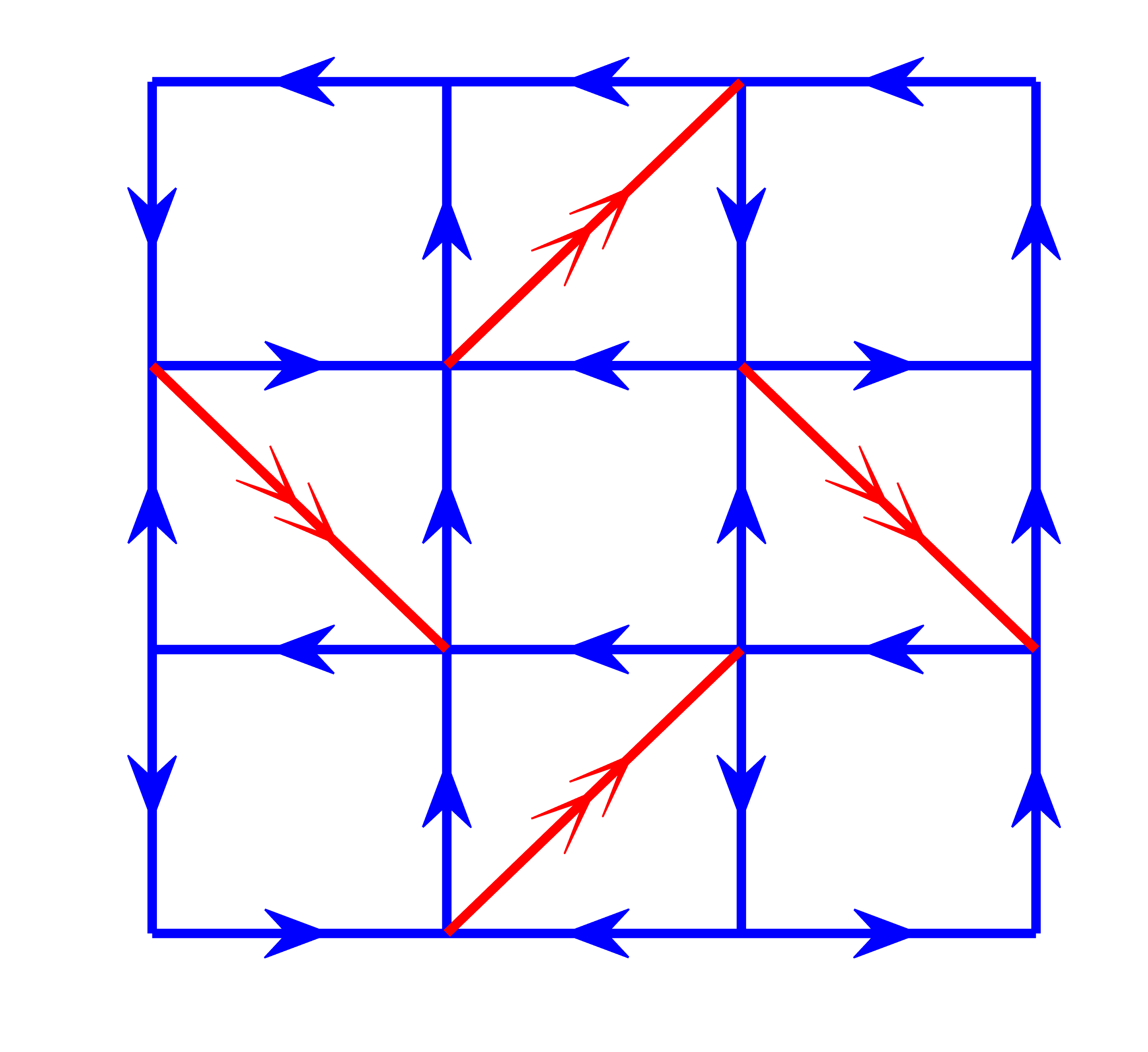
(a) $A$

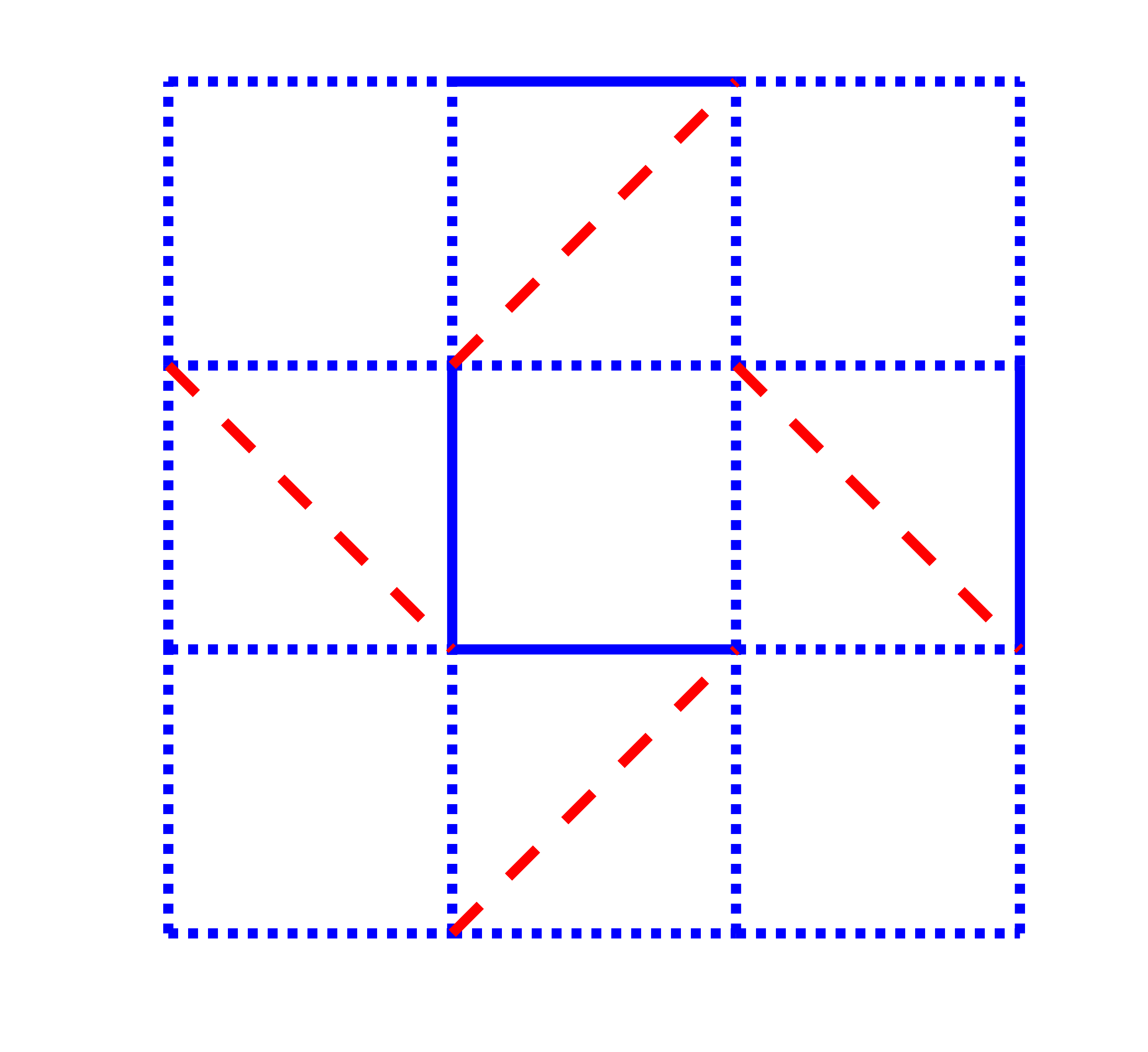
(b) $B$

Figure 7: The ansatz in dashed lines are 0. The ansatz $B$ are all real and in solid and dotted lines have opposite sign. It is 0-flux in empty square and $\pi$-flux in $J_{2}$ square.

For the $(p_{2},p_{4},p_{7})=(0,1,1)$ condition, we have

$$\phi_{T_{x}}(X,Y,s) = 0,$$ (70)

$$\phi_{T_{y}}(X,Y,s) = 0,$$ (71)

$$\phi_{C_{4}}(X,Y,s) = \delta_{s,0}\pi,$$ (72)

$$\phi_{\sigma}(X,Y,s) = \frac{\pi}{2}+\delta_{s,0}\pi.$$ (73)

The ansatz are $(\pi,\pi)$-flux, which is shown in Fig. 8

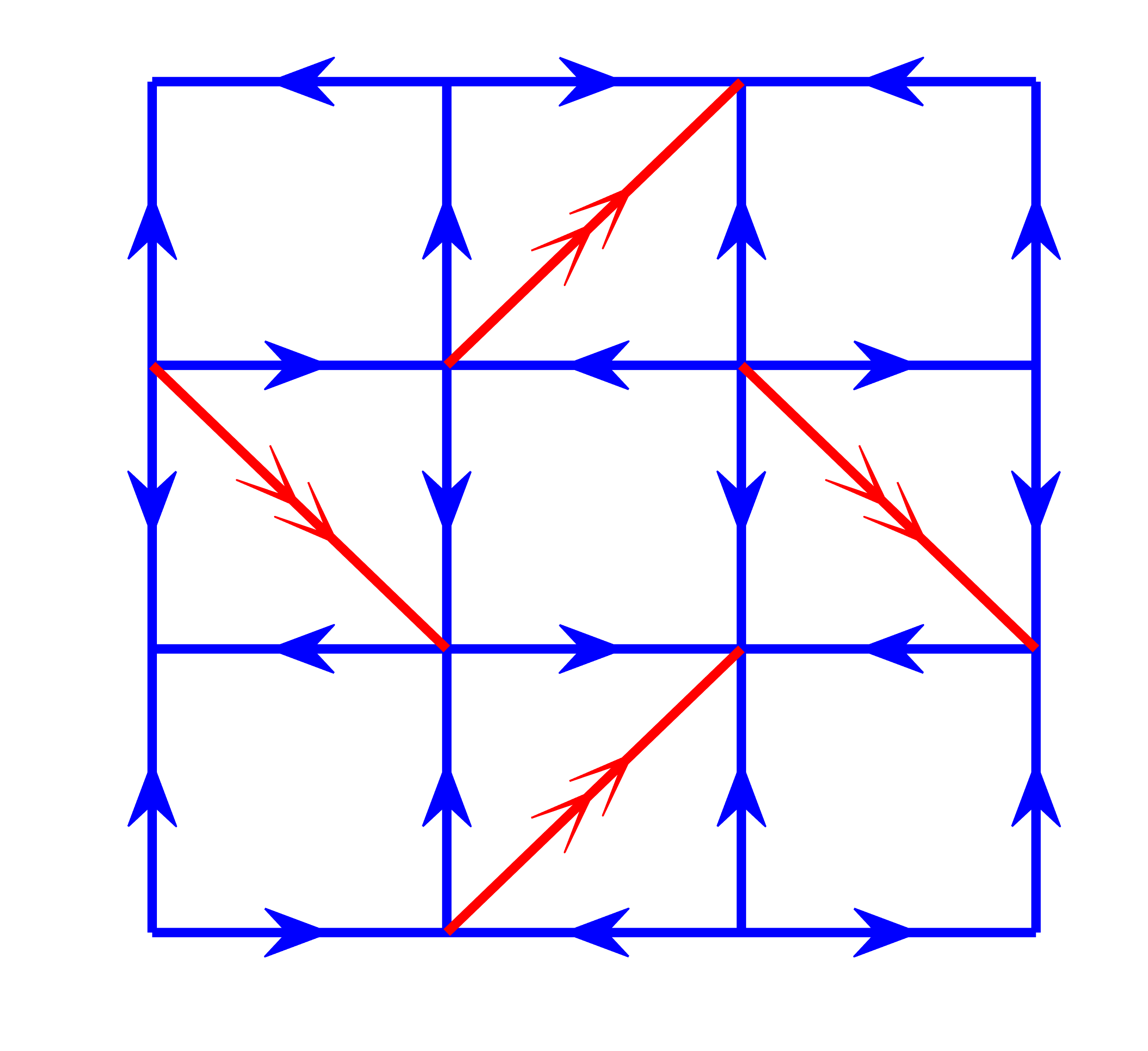
(a) $A$

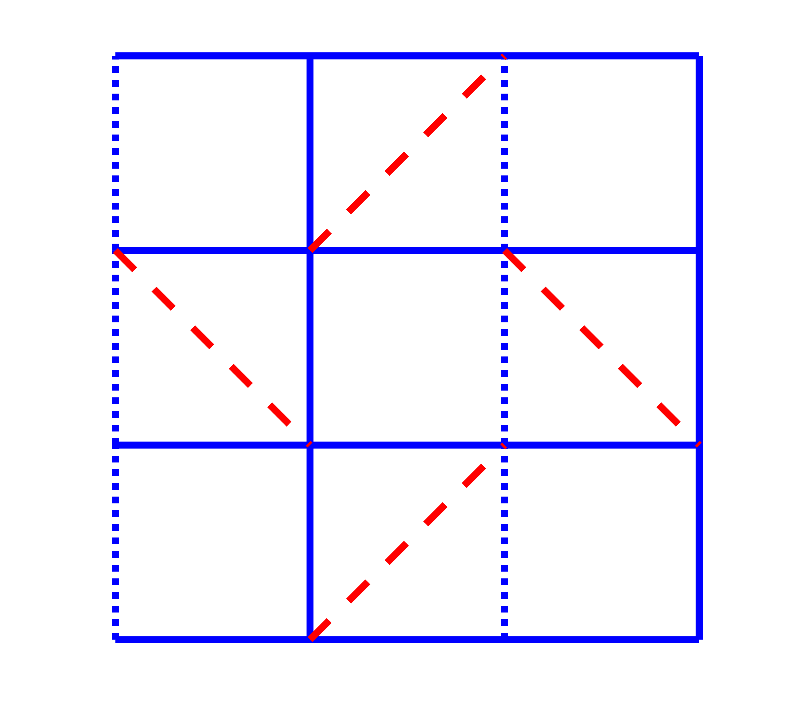
(b) $B$

Figure 8: The ansatz on dashed lines are 0. The ansatz $B$ are all real and on solid and dotted lines have opposite sign. It is $\pi$-flux in empty square and $\pi$-flux in $J_{2}$ square.

A.3 $A_{\rm n.n.n.}=0$ and $B_{\rm n.n.n.}\neq 0$

In this condition, $p_{2}+p_{4}=0$ and there are no constraint on $p_{7}$. Therefore, there are four types of possible ansatz.

First we consider $p_{2}=p_{4}=0$ condition. For $(p_{2},p_{4},p_{7})=(0,0,0)$ condition, the PSG solution is

$$\phi_{C_{4}}(X,Y,s) = 0,$$ (74)

$$\phi_{\sigma}(X,Y,s) = 0.$$ (75)

while $(p_{2},p_{4},p_{7})=(0,0,1)$ is

$$\phi_{C_{4}}(X,Y,s) = 0,$$ (76)

$$\phi_{\sigma}(X,Y,s) = \frac{\pi}{2}.$$ (77)

The ansatz of these two conditions are both $(0,0)$-flux and gauge equivalent, which are shown in Fig. 9.

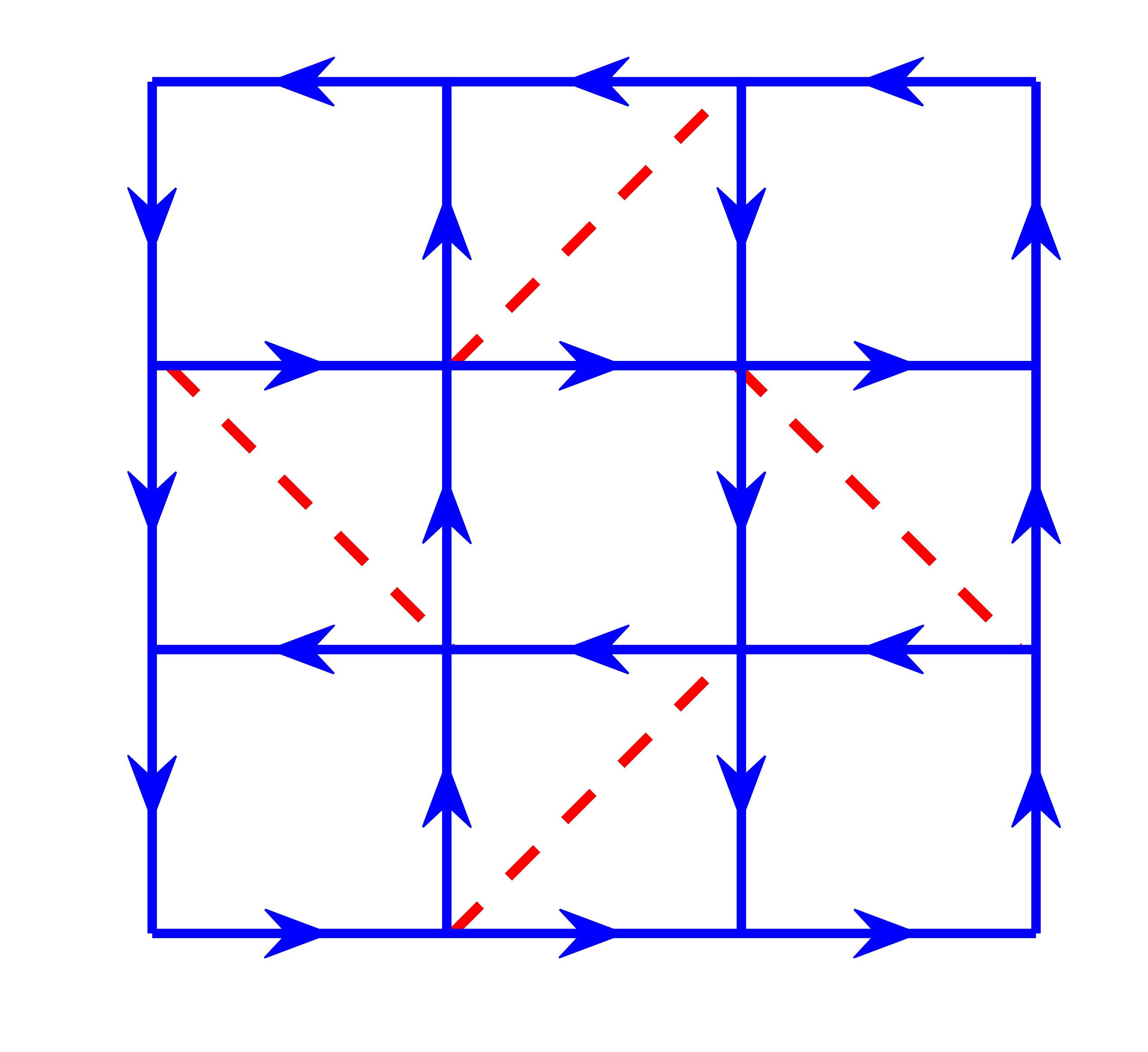
(a) $A$ of $(p_{2},p_{4},p_{7})=(0,0,0)$

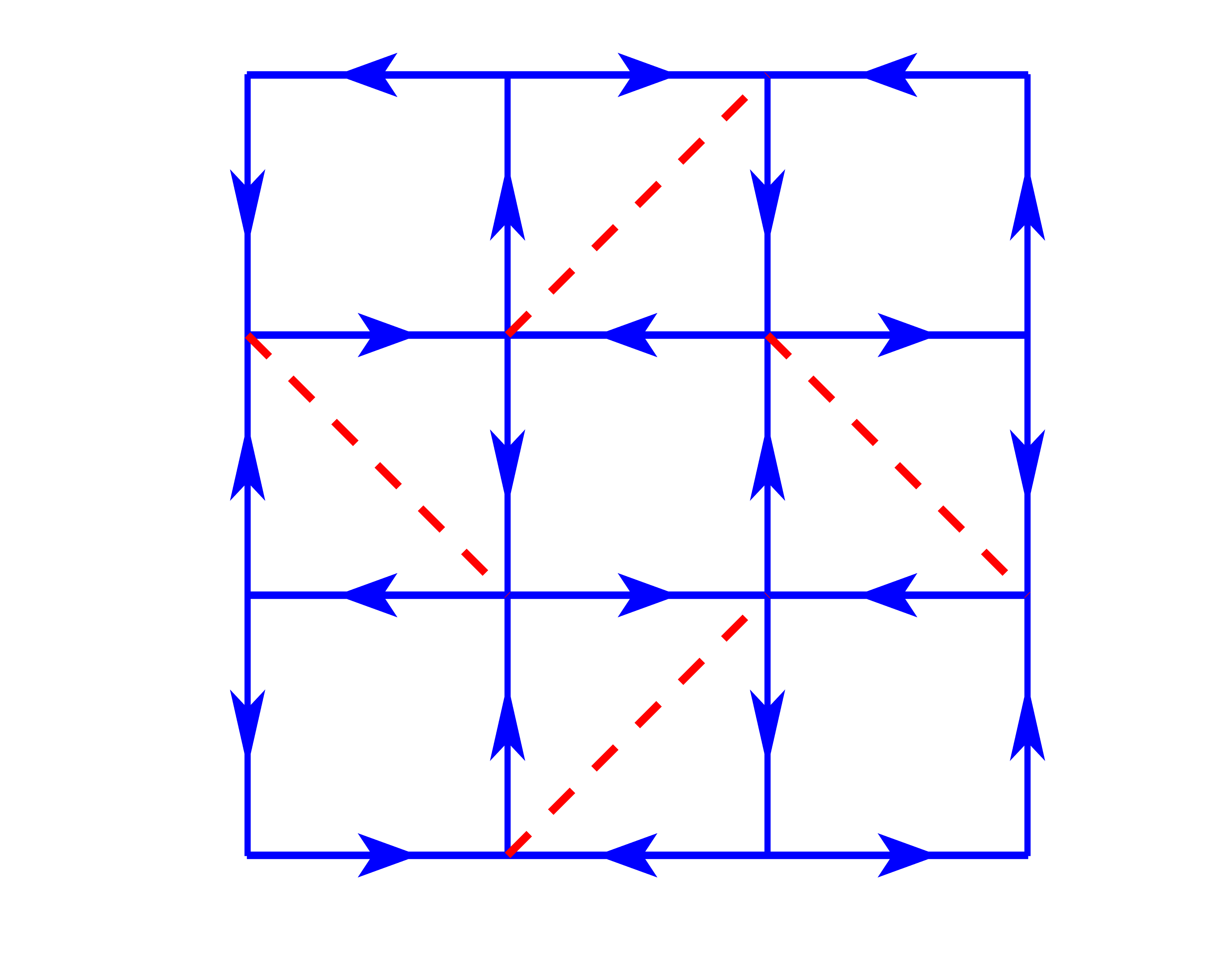
(b) $A$ of $(p_{2},p_{4},p_{7})=(0,0,1)$

Figure 9: The ansatz on dashed lines are 0. The two ansatz are gauge equivalent. It is $0$-flux in empty square and $0$-flux in $J_{2}$ square. $B_{\rm n.n}=0$ and $B_{\rm n.n.n}$ are real and uniform.

Then we consider $p_{2}=p_{4}=1$ condition. For $(p_{2},p_{4},p_{7})=(1,1,0)$ condition, the PSG solution is

$$\phi_{C_{4}}(X,Y,s) = Y\pi+\delta_{s,0},$$ (78)

$$\phi_{\sigma}(X,Y,s) = x_{s}y_{s}\pi+\delta_{s,0}\pi.$$ (79)

while $(p_{2},p_{4},p_{7})=(1,1,1)$ is

$$\phi_{C_{4}}(X,Y,s) = Y\pi+\delta_{s,0},$$ (80)

$$\phi_{\sigma}(X,Y,s) = \frac{\pi}{2}+x_{s}y_{s}\pi+\delta_{s,0}\pi.$$ (81)

The ansatz are both $(\pi,0)$-flux and also gauge equivalent.

A.4 Plaquette-singlet state

Now we consider the plaquette-singlet states, which break the glide symmetry and are out of the algebraic PSG solutions. After self-consistent calculation, we find only the zero-flux plaquette-singlet ansatz can be solved self-consistently, and the self-consistent solutions are such that only the ansatz($A$ and $B$) within the selected plaquettes are nonzero. Because there are two inequivalent plaquette (empty-square and $J_{2}$-square) in the Shastry-Sutherland lattice, only two inequivalent plaquette-singlet ansatz exist, which are shown in Fig. 10.

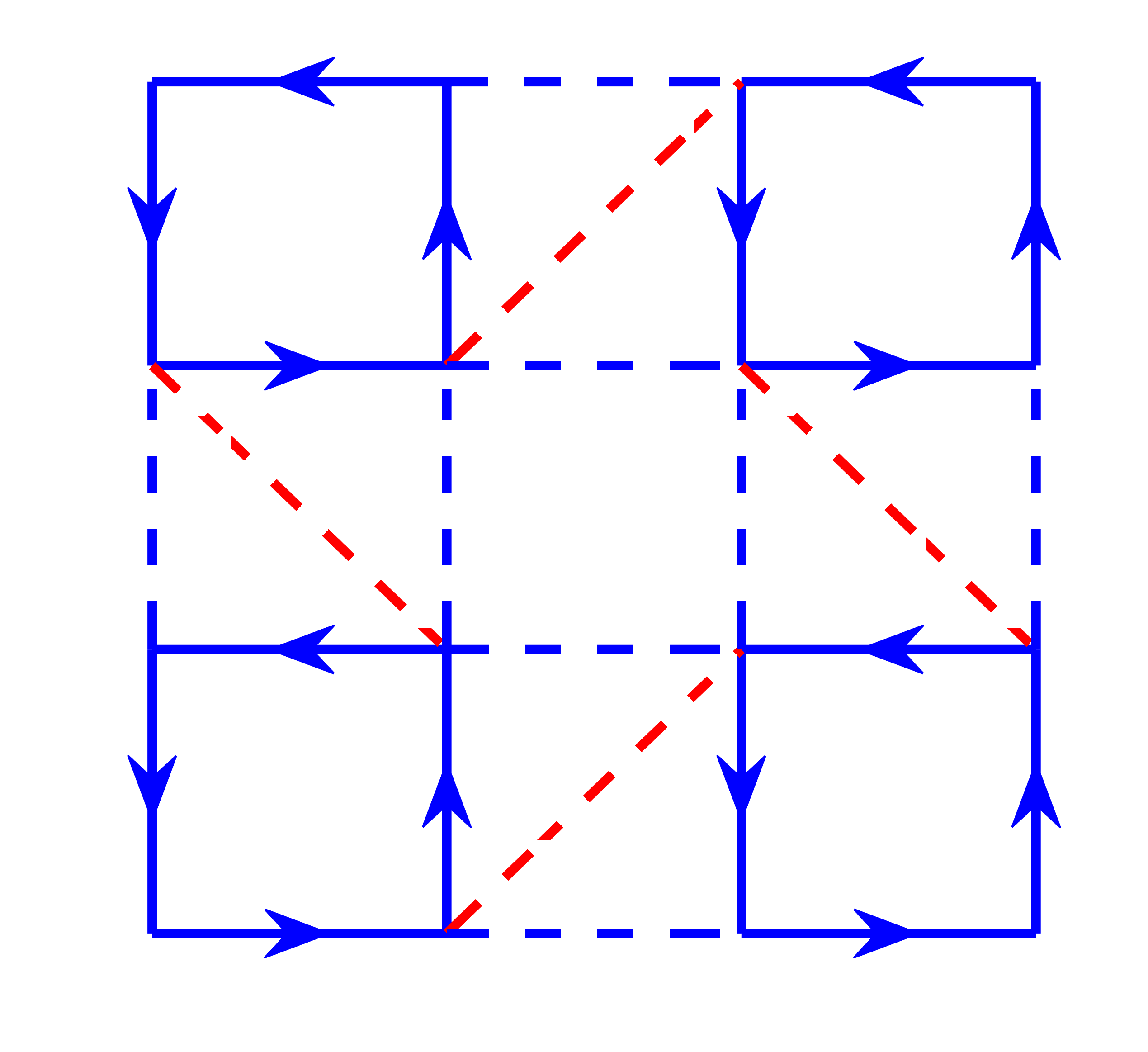
(a) $A$ of PS in empty-square

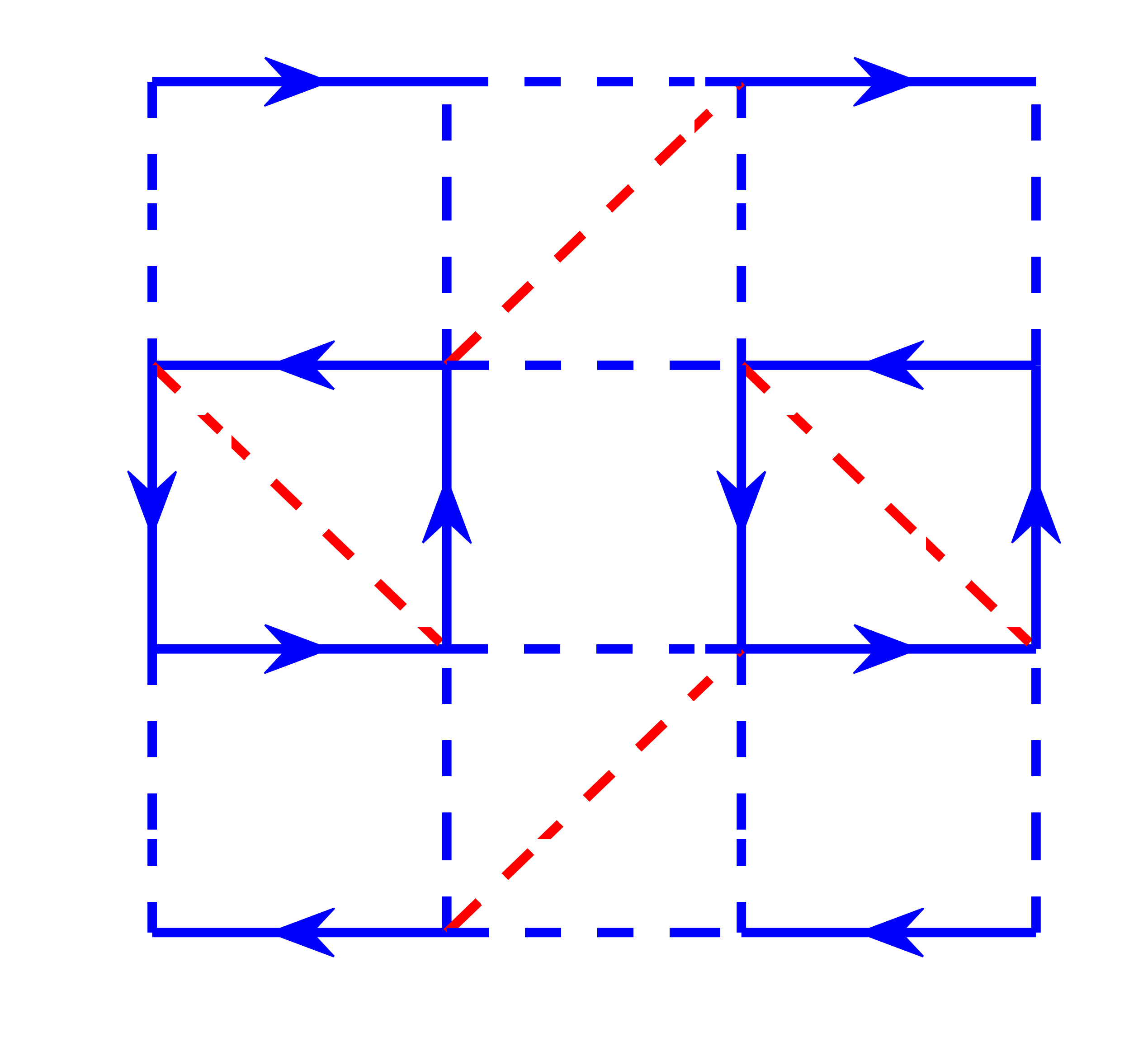
(b) $A$ of PS in $J_{2}$-square

Figure 10: The ansatz $A$ of plaquette-singlet state in (a) empty-square and (b) $J_{2}$-square. $B$ of the PS state in empty-square is always zero. For the $B$ of the PS state in $J_{2}$-square, only the $B_{2}$ in the $J_{2}$ bonds of the $J_{2}$-square is nonzero.

Appendix B Mean-field theory results

In this section we will show the properties of these four gauge inequivalent spin liquid states, including the ansatz amplitudes, spinon dispersions and the spin structure factors. The static structure factor is defined as

$$S(\mathbf{k})=\frac{1}{N_{s}}\sum_{i,j}\left\langle\mathbf{S}_{i}\cdot\mathbf{S}_{j}\right\rangle e^{i\mathbf{k}\cdot\left(\mathbf{r}_{i}-\mathbf{r}_{j}\right)},$$ (82)

while the dynamic structure factor is

$$S(\mathbf{k},\omega)=\frac{1}{N_{s}}\sum_{i,j}\left\langle\mathbf{S}_{i}(t)\cdot\mathbf{S}_{j}(0)\right\rangle e^{i\mathbf{k}\cdot\left(\mathbf{r}_{i}-\mathbf{r}_{j}\right)-i\omega t}.$$ (83)

In the Schwinger boson mean field theory, the structure factor can be expressed by the imaginary part of “bubble” Feynman diagrams. Note that the anomalous green’s function of the spinons also takes important parts. The static and dynamic spin structure factor can be measured experimentally by neutron scattering.

B.1 $(0,0)$-flux state

The mean-field Hamiltonian is shown in Eq. (7) in Main Text with the mean-field ansatz $A$ and $B$ shown in Fig. 9. If we choose the empty square as the unit cell, after Fourier transformation $b_{\mathbf{r}}=\frac{1}{\sqrt{N_{s}}}\sum_{\mathbf{r}}e^{-i\mathbf{k}\cdot\mathbf{r}}b_{\mathbf{k}}$, the mean-field Hamiltonian becomes

$$H_{\mathrm{MF}}=\sum_{\mathbf{k}}\Psi_{\mathbf{k}}^{\dagger}D_{\mathbf{k}}\Psi_{\mathbf{k}}+N_{s}\left[\mu+\mu\kappa+8J_{1}\left|A_{1}\right|^{2}-2J_{2}\left|B_{2}\right|^{2}\right],$$ (84)

where we have used the Nambu spinor $\Psi_{\mathbf{k}}=(b_{0\mathbf{k}\uparrow},b_{1\mathbf{k}\uparrow},b_{2\mathbf{k}\uparrow},b_{3\mathbf{k}\uparrow},b_{0\mathbf{-k}\downarrow}^{\dagger},b_{1\mathbf{-k}\downarrow}^{\dagger},b_{2\mathbf{-k}\downarrow}^{\dagger},b_{3\mathbf{-k}\downarrow}^{\dagger})^{T}$. The subscript $s=0,1,2,3$ in $b_{s\bm{k}\sigma}$ is the atom index in the unit cell, which is shown in Fig. 6. The $8\times 8$ matrix $D_{\mathbf{k}}$ satisfies

$$D_{\mathbf{k}} = -\mu\mathbf{1}+\left(\begin{array}[]{cc}\boldsymbol{B}_{\mathbf{k}}&\boldsymbol{A}_{\mathbf{k}}\\ \boldsymbol{A}_{\mathbf{k}}^{\dagger}&\boldsymbol{B}_{-\mathbf{k}}^{T}\end{array}\right),$$ (87)

where $\mathbf{1}$ is the $8\times 8$ identity matrix, and $\boldsymbol{A}_{\mathbf{k}}$ and $\boldsymbol{B}_{\mathbf{k}}$ are

$$\boldsymbol{A}_{\mathbf{k}} = \left(\begin{array}[]{cccc}0&\frac{1}{2}J_{1}A_{1}(-1+e^{-ik_{1}})&0&\frac{1}{2}J_{1}A_{1}(1-e^{-ik_{2}})\\ \frac{1}{2}J_{1}A_{1}(1-e^{ik_{1}})&0&\frac{1}{2}J_{1}A_{1}(-1+e^{-ik_{2}})&0\\ 0&\frac{1}{2}J_{1}A_{1}(1-e^{ik_{2}})&0&\frac{1}{2}J_{1}A_{1}(-1+e^{ik_{1}})\\ \frac{1}{2}J_{1}A_{1}(-1+e^{ik_{2}})&0&\frac{1}{2}J_{1}A_{1}(1-e^{-ik_{1}})&0\\ \end{array}\right),$$ (92)

$$\boldsymbol{B}_{\mathbf{k}} = \left(\begin{array}[]{cccccccc}0&0&\frac{1}{2}J_{2}B_{2}e^{-ik_{2}}&0\\ 0&0&0&\frac{1}{2}J_{2}B_{2}e^{ik_{1}}\\ \frac{1}{2}J_{2}B_{2}e^{ik_{2}}&0&0&0\\ 0&\frac{1}{2}J_{2}B_{2}e^{-ik_{1}}&0&0\end{array}\right).$$ (97)

After a Bogoliubov transformation, the mean-field Hamiltonian can be diagonalized as

$$H_{\mathrm{MF}}=\sum_{\mathbf{k}s}\omega_{s\mathbf{k}}(\gamma_{s\mathbf{k}\uparrow}^{\dagger}\gamma_{s\mathbf{k}\uparrow}+\gamma_{s\mathbf{k}\downarrow}^{\dagger}\gamma_{s\mathbf{k}\downarrow}+1)+N_{s}\left[\mu+\mu\kappa+8J_{1}\left|A_{1}\right|^{2}-2J_{2}\left|B_{2}\right|^{2}\right],$$ (98)

where the $\omega_{s\mathbf{k}}$ is the spinon dispersions, and $s=0,1,2,3$. The self-consistent equations are

$$16J_{1}A_{1} = -\sum_{s}\int_{BZ}\frac{\partial\omega_{s\mathbf{k}}}{\partial A_{1}}\mathbf{d}^{2}k,$$ (99)

$$4J_{2}B_{2} = \sum_{s}\int_{BZ}\frac{\partial\omega_{s\mathbf{k}}}{\partial B_{2}}\mathbf{d}^{2}k,$$ (100)

$$1+\kappa = -\sum_{s}\int_{BZ}\frac{\partial\omega_{s\mathbf{k}}}{\partial\mu}\mathbf{d}^{2}k,$$ (101)

where the integral is over the BZ. With these self-consistent equations, the mean-field ansatz can be solved. The spinon dispersion at critical spinon density $\kappa_{c}$ and the ansatz amplitudes and are shown in Fig. 11.

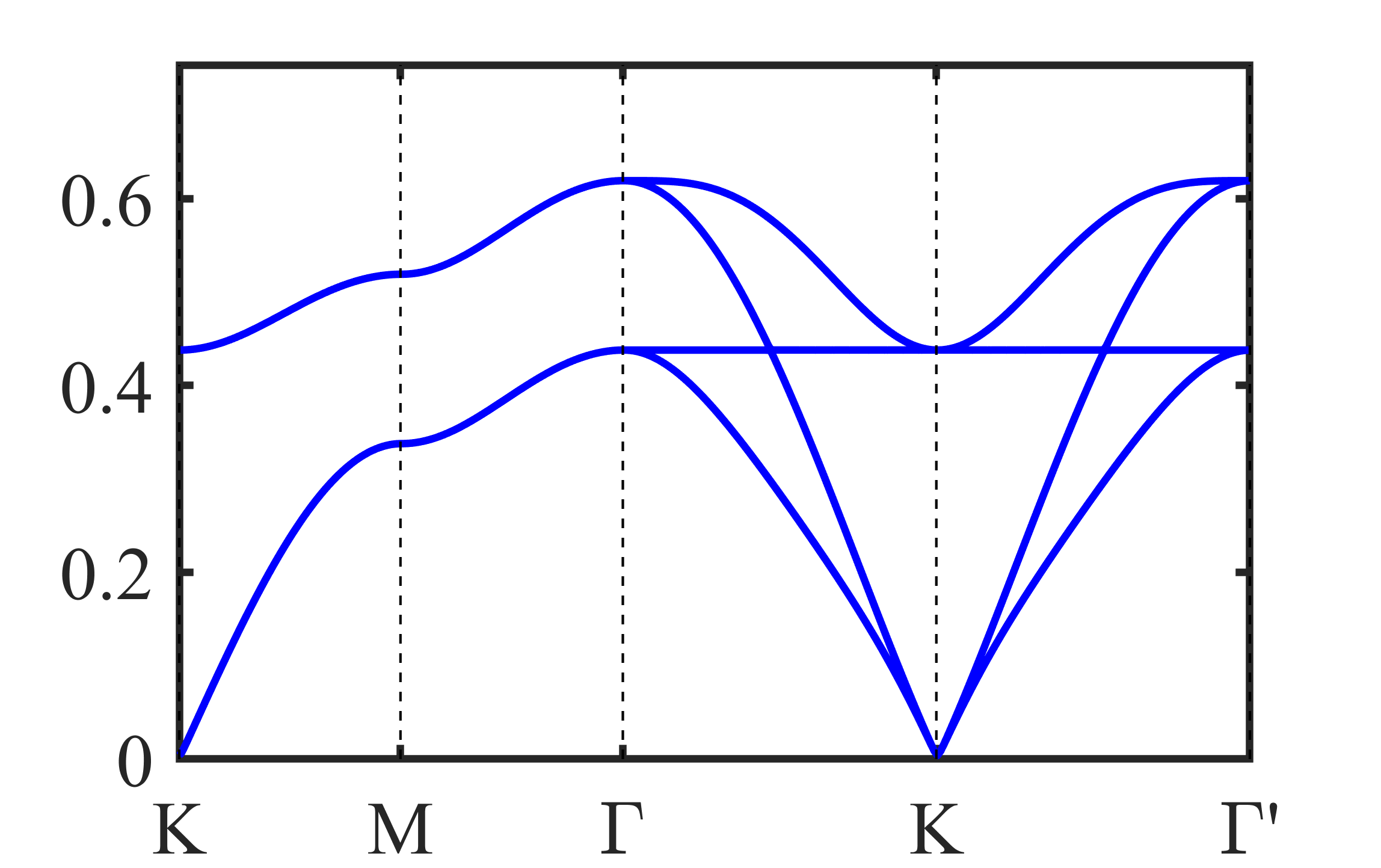
(a) Spinon dispersion at $\kappa_{c}$

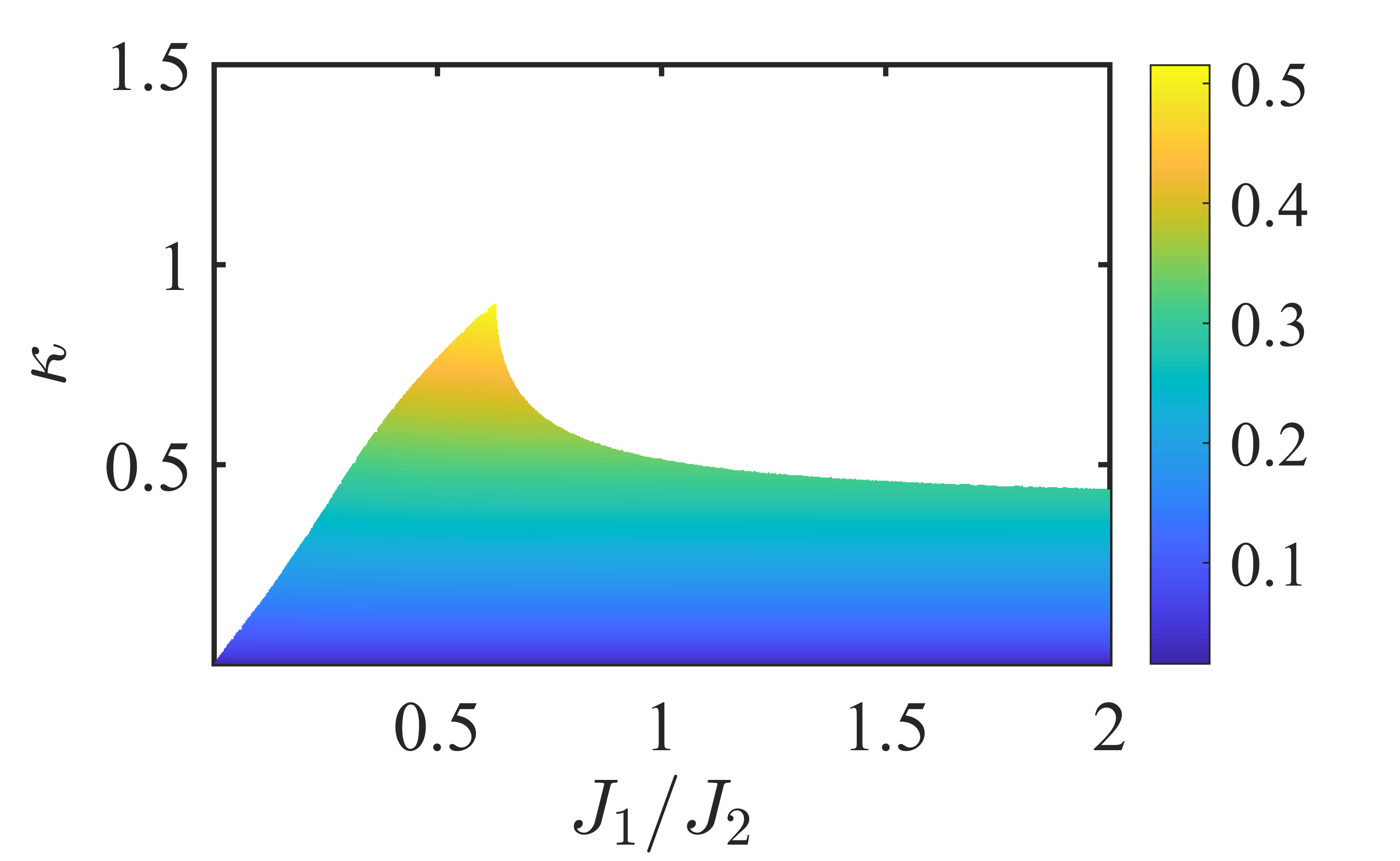
(b) $A_{1}$

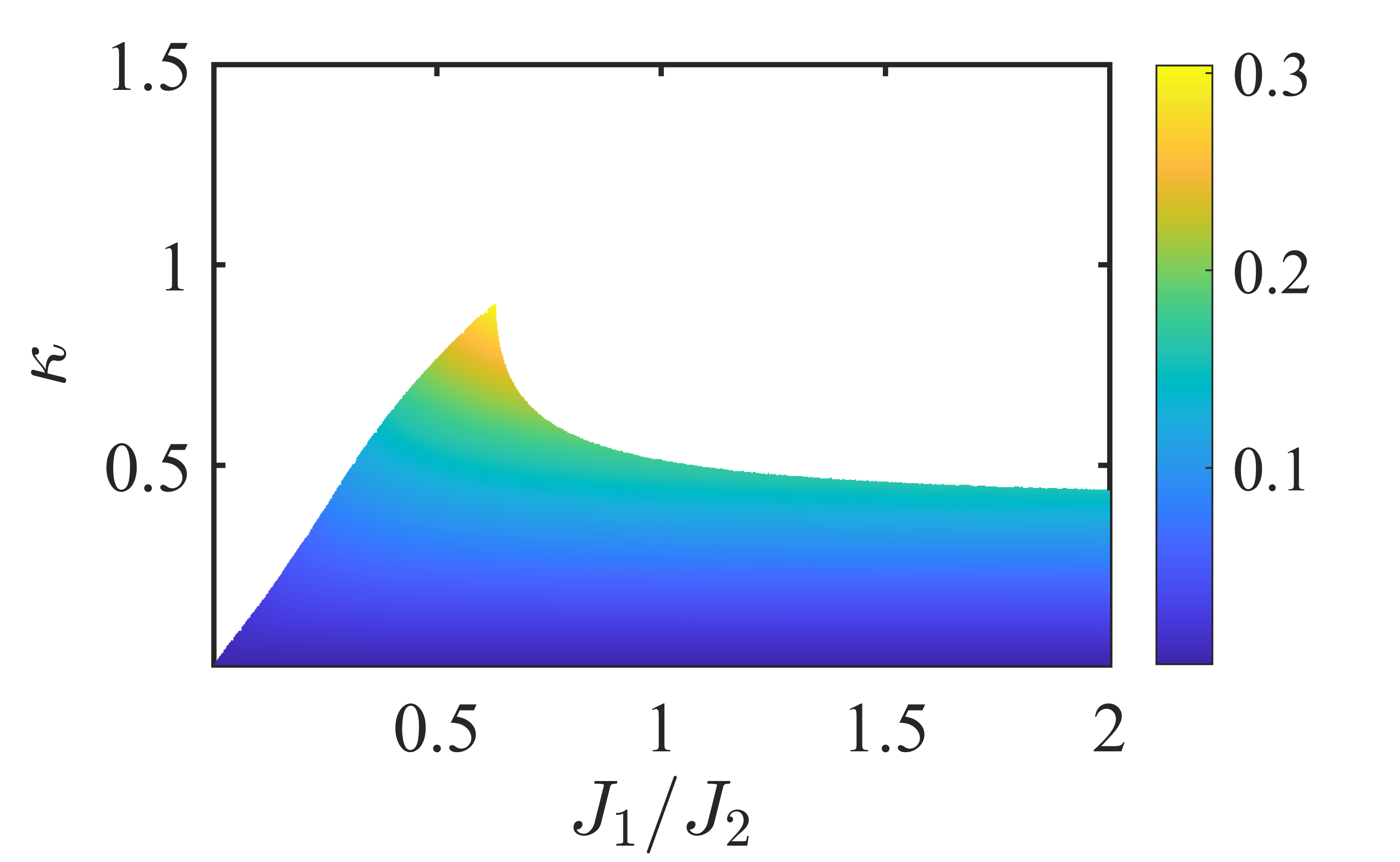
(c) $B_{2}$

Figure 11: (a) is the spinon dispersion at $\kappa=\kappa_{c}$ and $J_{1}=J_{2}=1$ of (0,0)-flux state. The plot path is shown in Fig. 1 (b) in Main Text. (b) and (c) are the ansatz $A_{1}$ and $B_{2}$ value respectively. $A_{2}$ and $B_{1}$ are always zero in these two conditions. The spinon condenses at the white area in (b) and (c).

As shown in Fig.11 (a), the minima of the spinon dispersion is located at $\mathbf{Q}=(\pi,\pi)$, and the gap vanishes at $\kappa=\kappa_{c}$. When $\kappa$ is larger than $\kappa_{c}$, the spinon will condense and form a magnetic order. The spinon condenses at the white area in Fig. 11 and the contour of the ansatz amplitudes indicate the critical $\kappa_{c}$. We find that $\kappa_{c}$ is always smaller than 1. Therefore, the (0,0)-flux state contributes to the magnetic ordered state in the physical condition. In the condition $\kappa<\kappa_{c}$, the IGG of this state is $U(1)$, and this state can not exist stably and always confines.

B.2 $(0,\pi)$-flux state

The mean-field Hamiltonian after Fourier transformation is

$$H_{\mathrm{MF}}=\sum_{\mathbf{k}}\Psi_{\mathbf{k}}^{\dagger}D_{\mathbf{k}}\Psi_{\mathbf{k}}+N_{s}\left[\mu+\mu\kappa+8J_{1}(\left|A_{1}\right|^{2}-\left|B_{1}\right|^{2})+2J_{2}\left|A_{2}\right|^{2}\right],$$ (102)

where

$$D_{\mathbf{k}} = -\mu\mathbf{1}+\left(\begin{array}[]{cc}\boldsymbol{B}_{\mathbf{k}}&\boldsymbol{A}_{\mathbf{k}}\\ \boldsymbol{A}_{\mathbf{k}}^{\dagger}&\boldsymbol{B}_{-\mathbf{k}}^{T}\end{array}\right),$$ (105)

and

$$\boldsymbol{A}_{\mathbf{k}} = \left(\begin{array}[]{cccc}0&\frac{1}{2}J_{1}A_{1}(-1-e^{-ik_{1}})&-\frac{1}{2}J_{2}A_{2}e^{-ik_{2}}&\frac{1}{2}J_{1}A_{1}(1+e^{-ik_{2}})\\ \frac{1}{2}J_{1}A_{1}(1+e^{ik_{1}})&0&\frac{1}{2}J_{1}A_{1}(-1+e^{-ik_{2}})&-\frac{1}{2}J_{2}A_{2}e^{ik_{1}}\\ \frac{1}{2}J_{2}A_{2}e^{ik_{2}}&\frac{1}{2}J_{1}A_{1}(1-e^{ik_{2}})&0&\frac{1}{2}J_{1}A_{1}(-1+e^{ik_{1}})\\ \frac{1}{2}J_{1}A_{1}(-1-e^{ik_{2}})&\frac{1}{2}J_{2}A_{2}e^{-ik_{1}}&\frac{1}{2}J_{1}A_{1}(1-e^{-ik_{1}})&0\\ \end{array}\right),$$ (110)

$$\boldsymbol{B}_{\mathbf{k}} = \left(\begin{array}[]{cccccccc}0&\frac{1}{2}B_{1}(-1-e^{-ik_{1}})&0&\frac{1}{2}B_{1}(-1-e^{-ik_{2}})\\ \frac{1}{2}B_{1}(-1-e^{ik_{1}})&0&\frac{1}{2}B_{1}(-1+e^{-ik_{2}})&0\\ 0&\frac{1}{2}B_{1}(-1+e^{ik_{2}})&0&\frac{1}{2}B_{1}(-1+e^{ik_{1}})\\ \frac{1}{2}B_{1}(-1-e^{ik_{2}})&0&\frac{1}{2}B_{1}(-1+e^{-ik_{1}})&0\end{array}\right).$$ (115)

And we have also used the Nambu spinor $\Psi_{\mathbf{k}}=(b_{0\mathbf{k}\uparrow},b_{1\mathbf{k}\uparrow},b_{2\mathbf{k}\uparrow},b_{3\mathbf{k}\uparrow},b_{0\mathbf{-k}\downarrow}^{\dagger},b_{1\mathbf{-k}\downarrow}^{\dagger},b_{2\mathbf{-k}\downarrow}^{\dagger},b_{3\mathbf{-k}\downarrow}^{\dagger})^{T}$. The Hamiltonian can be diagonalized by a Bogoliubov transformation, which yields

$$H_{\mathrm{MF}}=\sum_{\mathbf{k}s}\omega_{s\mathbf{k}}(\gamma_{s\mathbf{k}\uparrow}^{\dagger}\gamma_{s\mathbf{k}\uparrow}+\gamma_{s\mathbf{k}\downarrow}^{\dagger}\gamma_{s\mathbf{k}\downarrow}+1)+N_{s}\left[\mu+\mu\kappa+8J_{1}(\left|A_{1}\right|^{2}-\left|B_{1}\right|^{2})+2J_{2}\left|A_{2}\right|^{2}\right],$$ (116)

and the self-consistent equations are

$$16J_{1}A_{1} = -\sum_{s}\int_{BZ}\frac{\partial\omega_{s\mathbf{k}}}{\partial A_{1}}\mathbf{d}^{2}k,$$ (117)

$$4J_{2}A_{2} =- \sum_{s}\int_{BZ}\frac{\partial\omega_{s\mathbf{k}}}{\partial A_{2}}\mathbf{d}^{2}k,$$ (118)

$$16J_{1}B_{1} = -\sum_{s}\int_{BZ}\frac{\partial\omega_{s\mathbf{k}}}{\partial B_{1}}\mathbf{d}^{2}k,$$ (119)

$$1+\kappa = -\sum_{s}\int_{BZ}\frac{\partial\omega_{s\mathbf{k}}}{\partial\mu}\mathbf{d}^{2}k,$$ (120)

Solving these self-consistent equations we have get the ansatz amplitudes, which are shown in Fig. 7.

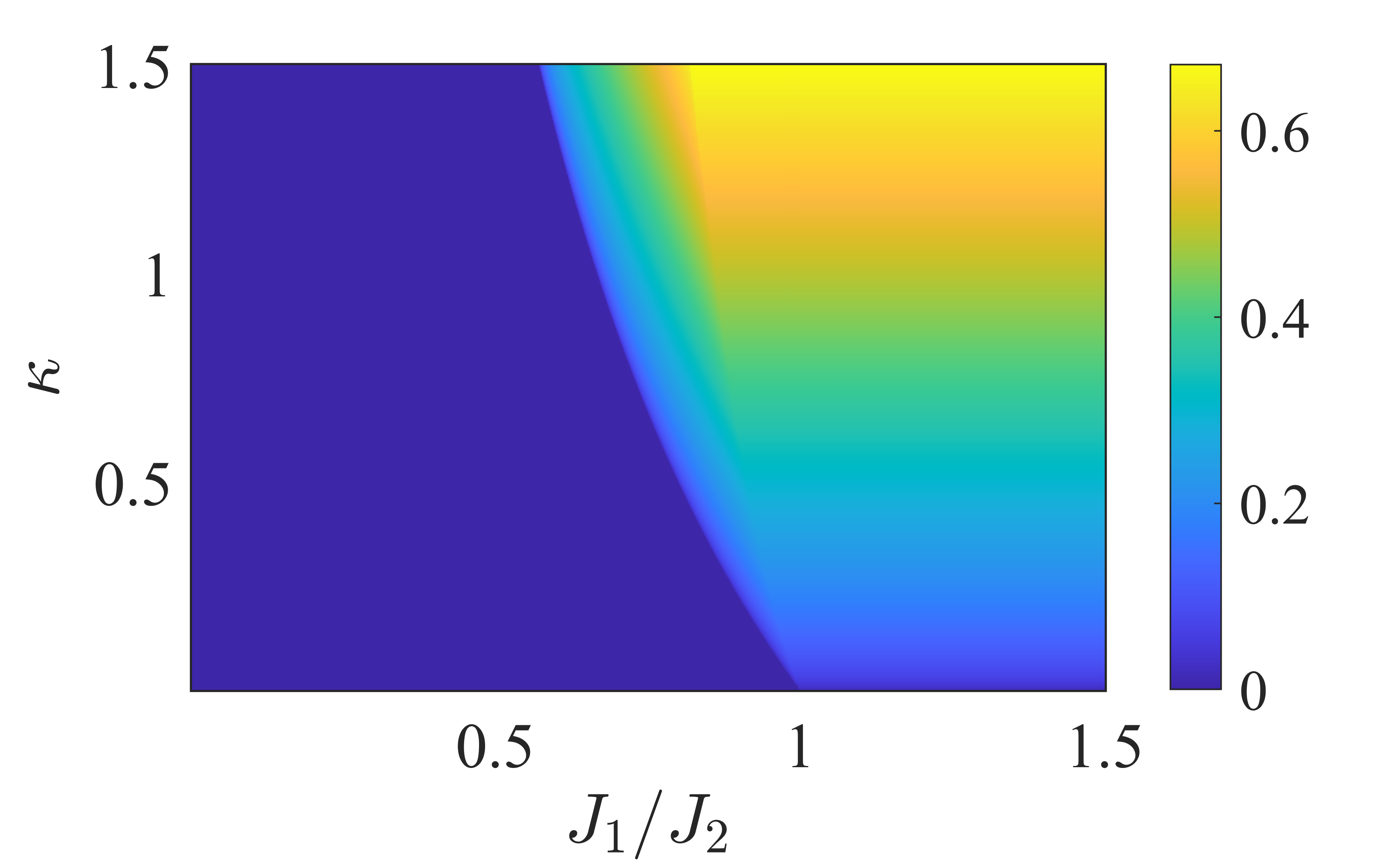
(a) $A_{1}$

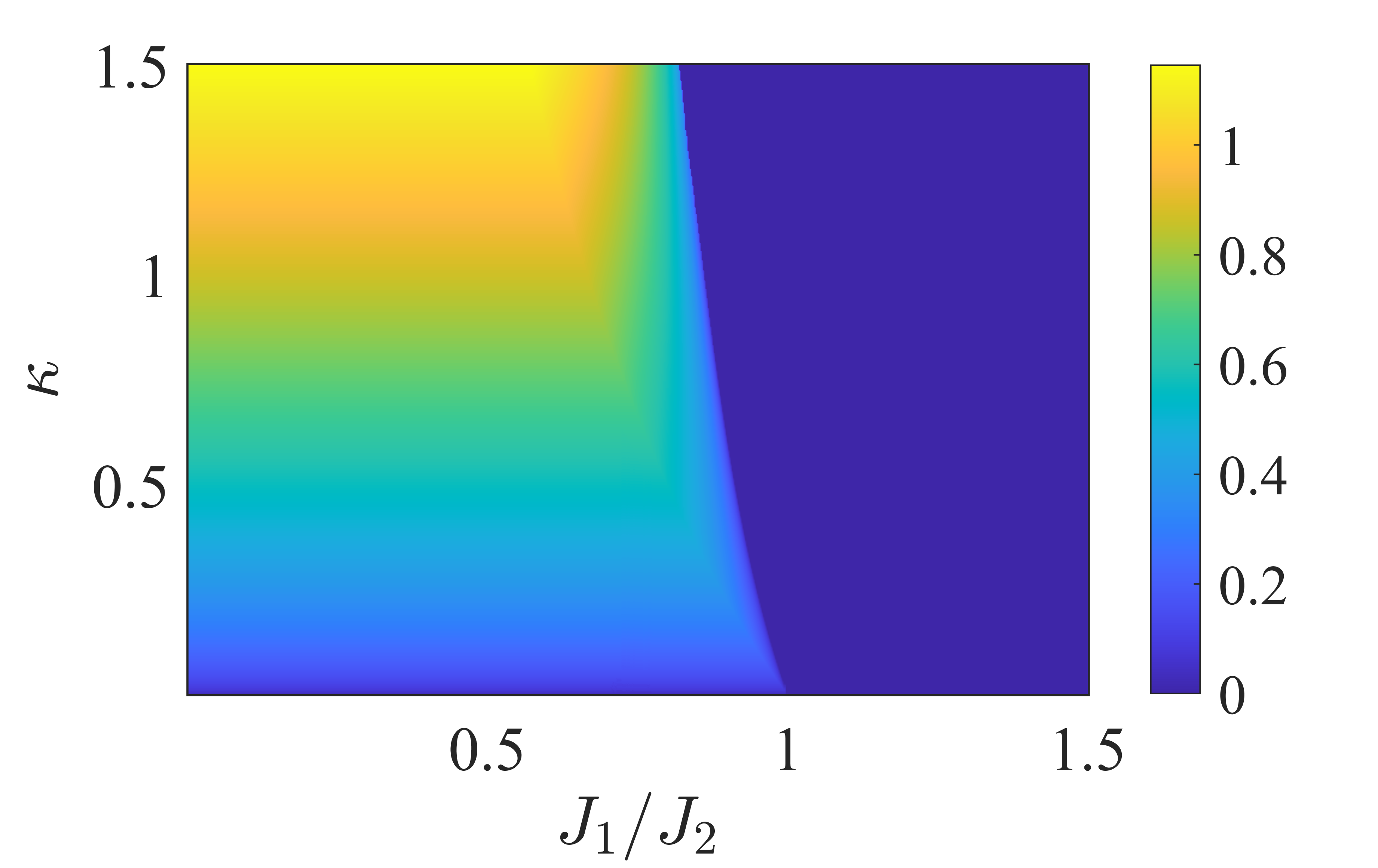
(b) $A_{2}$

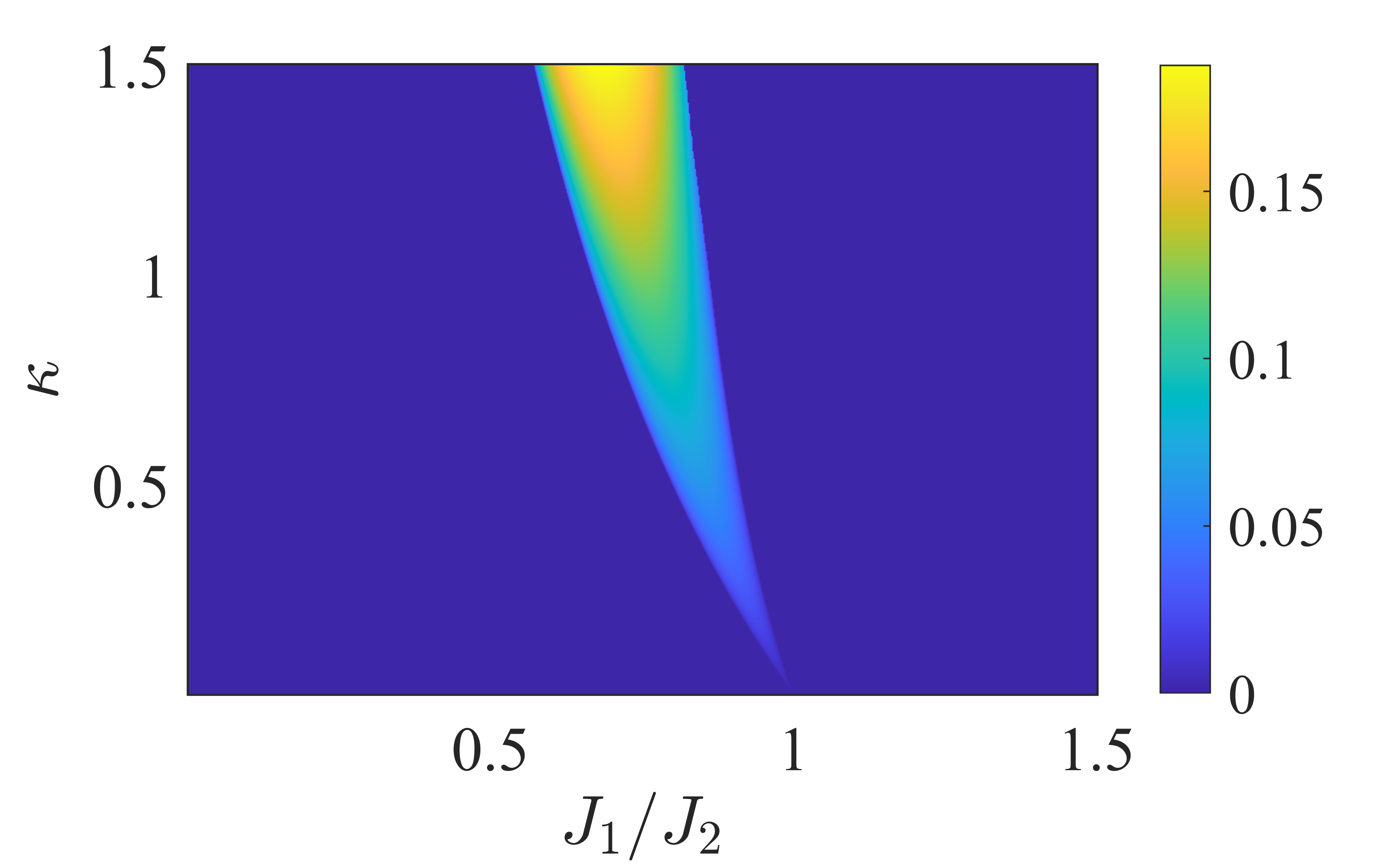
(c) $B_{1}$

Figure 12: The ansatz value (a) $A_{1}$, (b) $A_{2}$ and (c) $B_{1}$ of $(0,\pi)$-flux. $A_{1}$ is finite at $J_{1}$ is large and $A_{2}$ is large at $J_{1}$ is large. $B_{1}$ is finite only when $A_{1}$ and $A_{2}$ are both finite. $B_{2}$ is always zero in this condition.

With these ansatz values, the spinon dispersion and the structure factor can be obtained, which are shown in Fig. 13. We find the bottom branch of the spinon dispersion is flat, therefore, the critical spinon density $\kappa_{c}$ is large in this state.

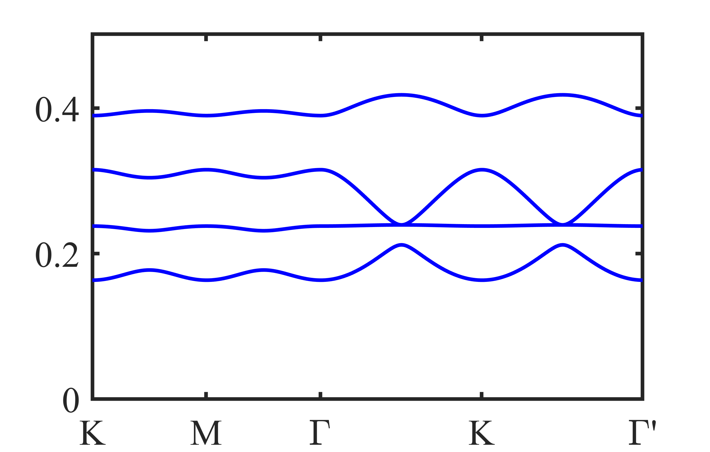
(a) Spinon dispersion

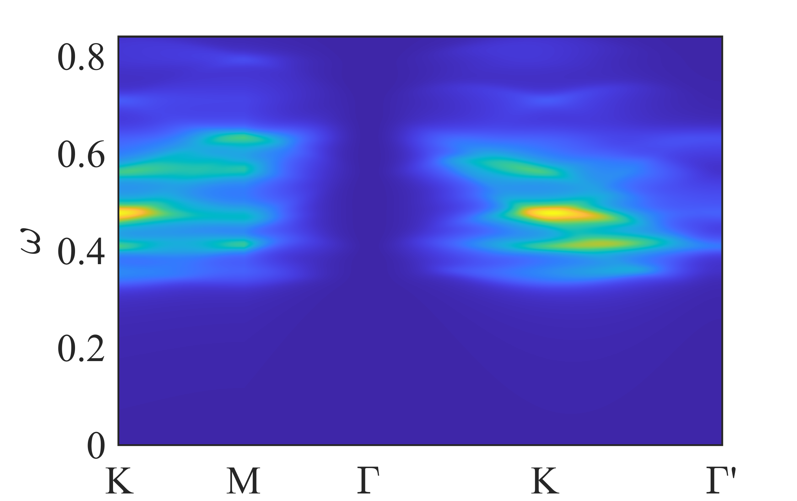
(b) dynamic structure factor

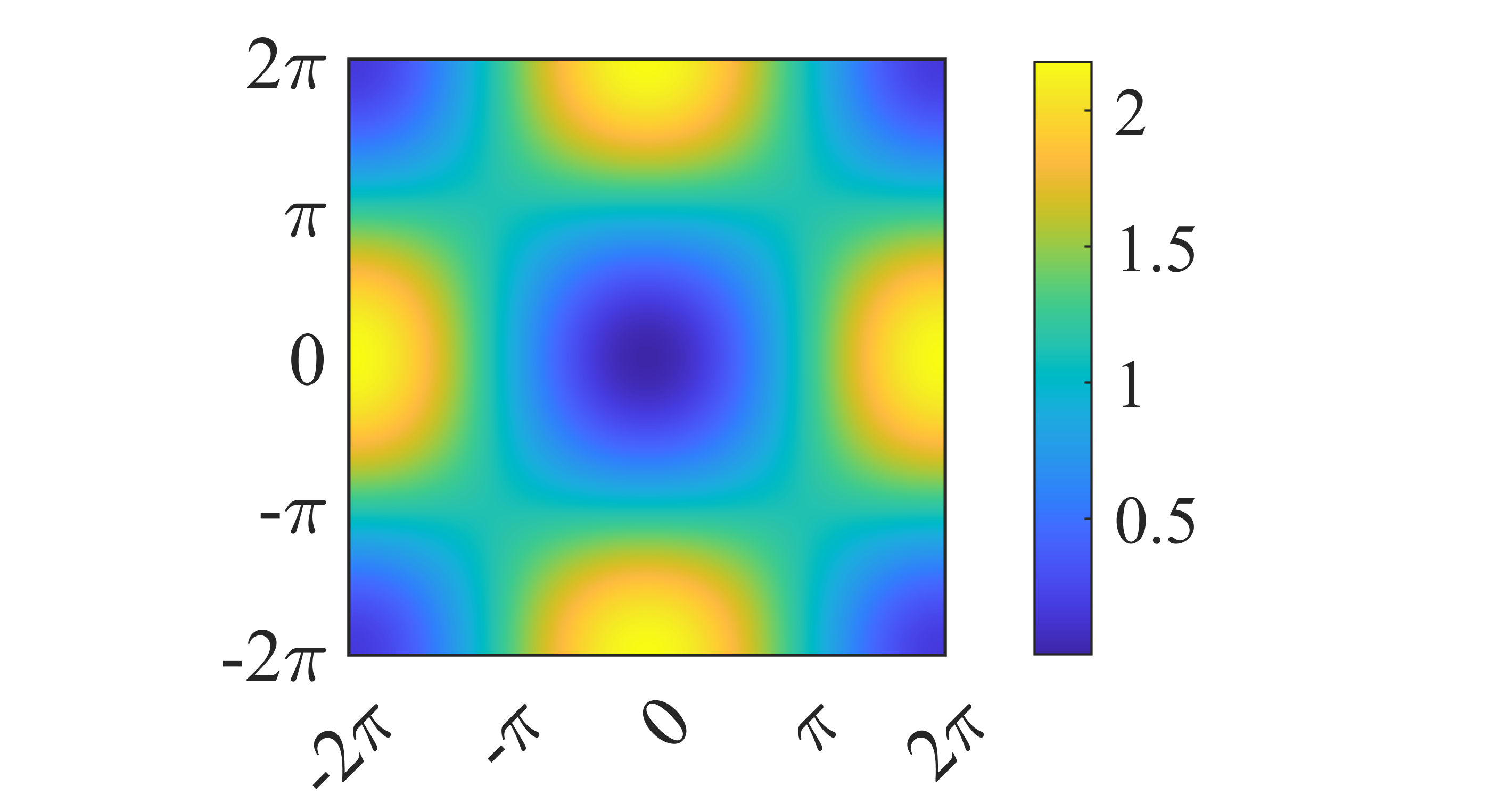
(c) static structure factor

Figure 13: (a) is the spinon dispersion, (b) is the dynamic structure factor, and (c) is the static structure factor of $(0,\pi)$-flux state ($J_{1}/J_{2}=0.7$). The plot path of (a) and (b) is shown in Fig. 1 (b) in Main Text.

The ground state energy of this state is slightly higher than the energy minimum of $\pi$-flux ($(\pi,\pi)$-flux) and zero-flux ((0,0)-flux) state as shown in Fig. (2)(c) in Main Text, therefore, this state is not shown in the phase diagram in Fig. 1 (c) in Main Text. However, the energy difference of $(\pi,\pi)$ and $(0,\pi)$-flux state is very small. Therefore, this state may also exist beyond the mean-field level.

B.3 $(\pi,0)$-flux state

The mean-field Hamiltonian of the $(\pi,0)$-flux state in the momentum space is

$$H_{\mathrm{MF}}=\sum_{\mathbf{k}}\Psi_{\mathbf{k}}^{\dagger}D_{\mathbf{k}}\Psi_{\mathbf{k}}+N_{s}\left[\mu+\mu\kappa+8J_{1}\left|A_{1}\right|^{2}-2J_{2}\left|B_{2}\right|^{2}\right],$$ (121)

where

$$D_{\mathbf{k}} = -\mu\mathbf{1}+\left(\begin{array}[]{cc}\boldsymbol{B}_{\mathbf{k}}&\boldsymbol{A}_{\mathbf{k}}\\ \boldsymbol{A}_{\mathbf{k}}^{\dagger}&\boldsymbol{B}_{-\mathbf{k}}^{T}\end{array}\right),$$ (124)

and

$$\boldsymbol{A}_{\mathbf{k}} = \left(\begin{array}[]{cccc}0&\frac{1}{2}J_{1}A_{1}(-1-e^{-ik_{1}})&0&\frac{1}{2}J_{1}A_{1}(-1-e^{-ik_{2}})\\ \frac{1}{2}J_{1}A_{1}(1+e^{ik_{1}})&0&\frac{1}{2}J_{1}A_{1}(-1+e^{-ik_{2}})&0\\ 0&\frac{1}{2}J_{1}A_{1}(1-e^{ik_{2}})&0&\frac{1}{2}J_{1}A_{1}(-1+e^{ik_{1}})\\ \frac{1}{2}J_{1}A_{1}(1+e^{ik_{2}})&0&\frac{1}{2}J_{1}A_{1}(1-e^{-ik_{1}})&0\\ \end{array}\right),$$ (129)

$$\boldsymbol{B}_{\mathbf{k}} = \left(\begin{array}[]{cccccccc}0&0&\frac{1}{2}J_{2}B_{2}e^{-ik_{2}}&0\\ 0&0&0&\frac{1}{2}J_{2}B_{2}e^{ik_{1}}\\ \frac{1}{2}J_{2}B_{2}e^{ik_{2}}&0&0&0\\ 0&\frac{1}{2}J_{2}B_{2}e^{-ik_{1}}&0&0\end{array}\right).$$ (134)

And we have also used the Nambu spinor $\Psi_{\mathbf{k}}=(b_{0\mathbf{k}\uparrow},b_{1\mathbf{k}\uparrow},b_{2\mathbf{k}\uparrow},b_{3\mathbf{k}\uparrow},b_{0\mathbf{-k}\downarrow}^{\dagger},b_{1\mathbf{-k}\downarrow}^{\dagger},b_{2\mathbf{-k}\downarrow}^{\dagger},b_{3\mathbf{-k}\downarrow}^{\dagger})^{T}$. After a Bogoliubov transformation, the mean-field Hamiltonian is diagonalized as

$$H_{\mathrm{MF}}=\sum_{\mathbf{k}s}\omega_{s\mathbf{k}}(\gamma_{s\mathbf{k}\uparrow}^{\dagger}\gamma_{s\mathbf{k}\uparrow}+\gamma_{s\mathbf{k}\downarrow}^{\dagger}\gamma_{s\mathbf{k}\downarrow}+1)+N_{s}\left[\mu+\mu\kappa+8J_{1}\left|A_{1}\right|^{2}-2J_{2}\left|B_{2}\right|^{2}\right],$$ (135)

where the $\omega_{s\mathbf{k}}$ is the spinon dispersions, and $s=0,1,2,3$. The self-consistent equations are

$$16J_{1}A_{1} = -\sum_{s}\int_{BZ}\frac{\partial\omega_{s\mathbf{k}}}{\partial A_{1}}\mathbf{d}^{2}k,$$ (136)

$$4J_{2}B_{2} = \sum_{s}\int_{BZ}\frac{\partial\omega_{s\mathbf{k}}}{\partial B_{2}}\mathbf{d}^{2}k,$$ (137)

$$1+\kappa = -\sum_{s}\int_{BZ}\frac{\partial\omega_{s\mathbf{k}}}{\partial\mu}\mathbf{d}^{2}k.$$ (138)

With these self-consistent equations, the mean-field ansatz can be solved. The spinon dispersion at physical condition $\kappa=1$ and the ansatz amplitudes and are shown in Fig. 14.

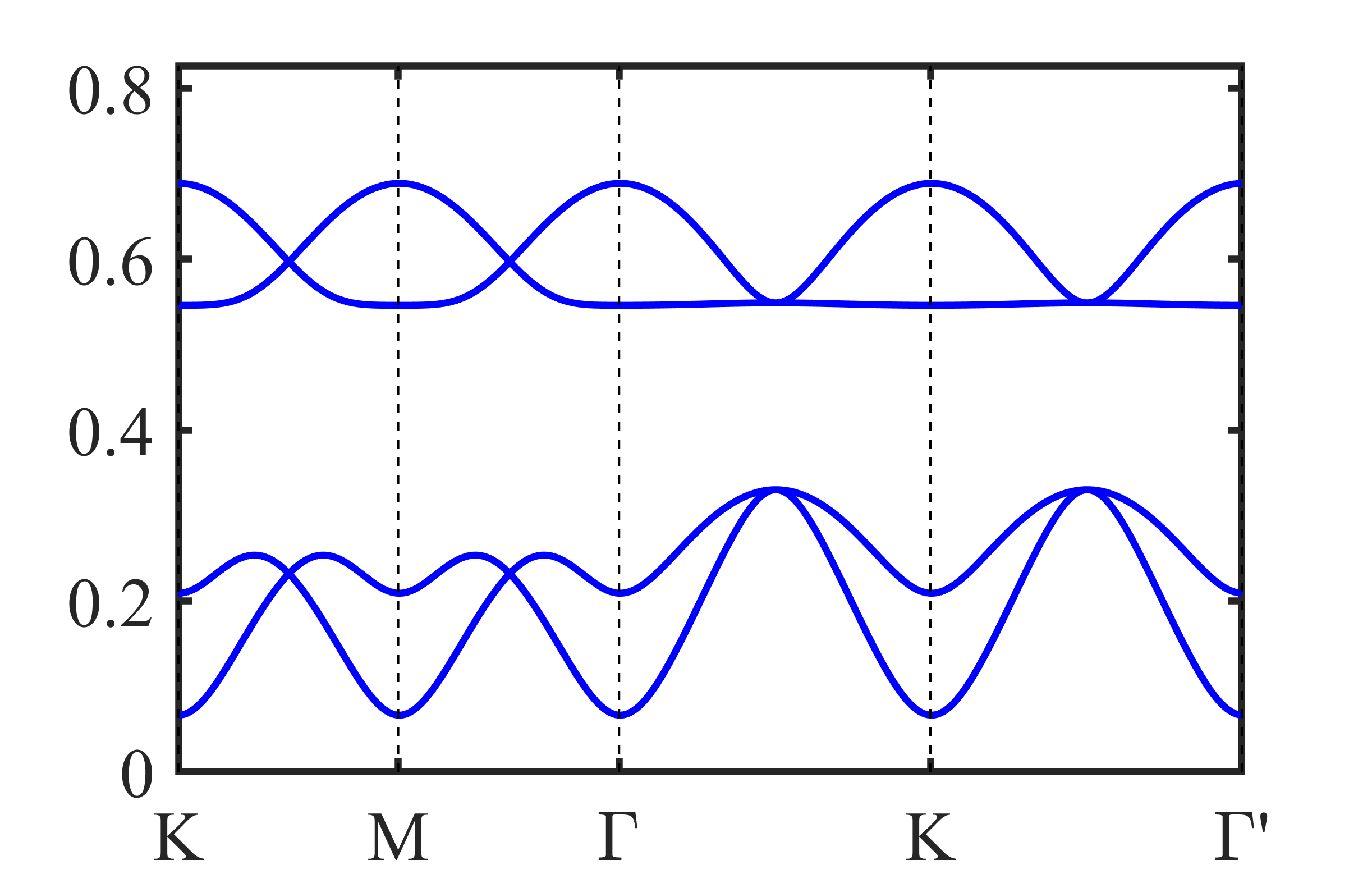
(a) Spinon dispersion at $\kappa=1$

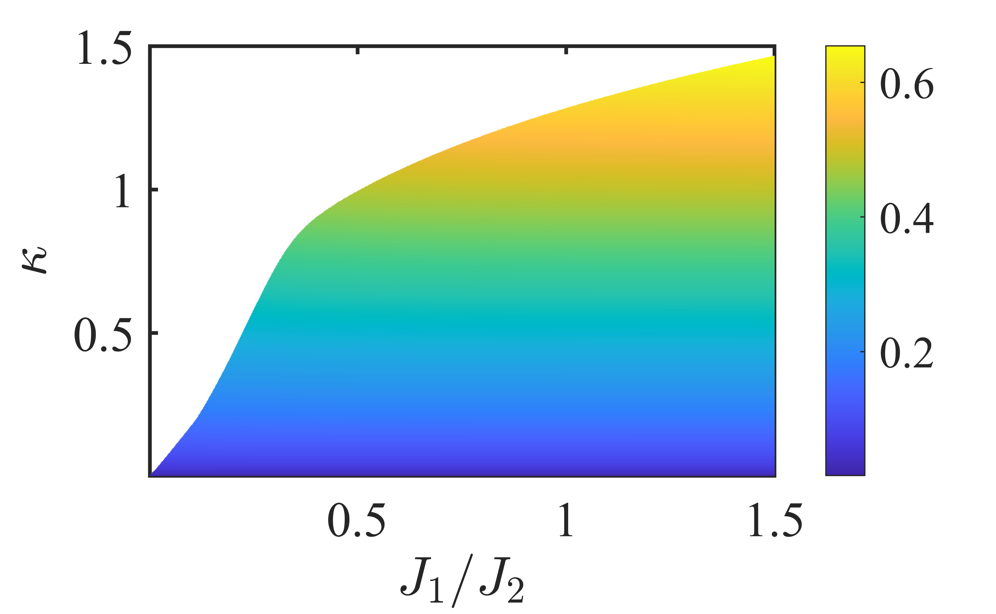
(b) $A_{1}$

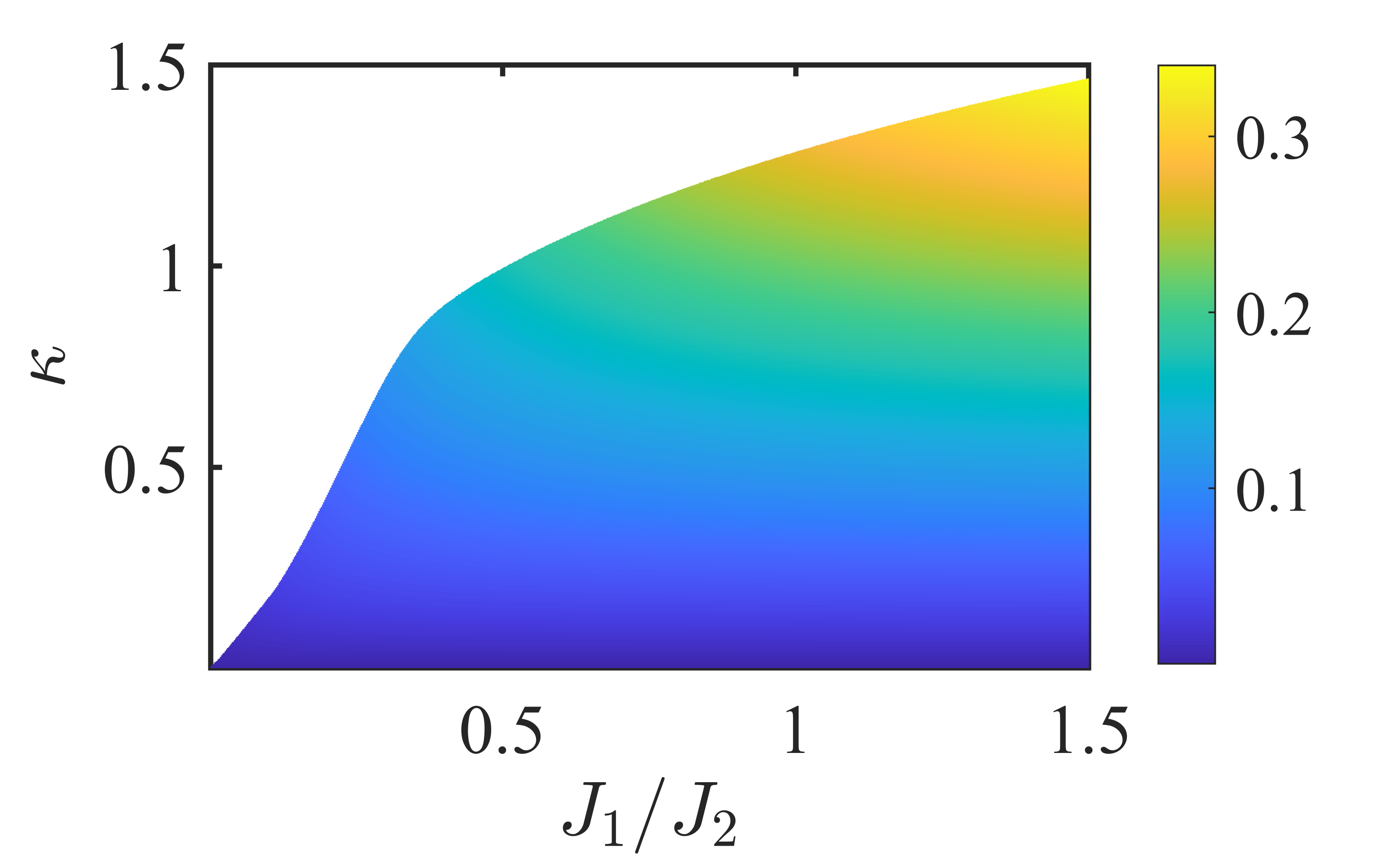
(c) $B_{2}$

Figure 14: (a) is the spinon dispersion at $\kappa=\kappa_{c}$ and $J_{1}=J_{2}=1$ of ($\pi,0$)-flux. The plot path is shown in Fig. 1 (b) in Main Text. (b) and (c) are the ansatz $A_{1}$ and $B_{2}$ value respectively. $A_{2}$ and $B_{1}$ are always zero in this condition.

As shown in Fig. 2 (c) in the Main Text, the ground state energy of this $(\pi,0)$-flux is much larger than the $(0,0)$-flux, which may not exist even beyond the mean field level.

B.4 $(\pi,\pi)$-flux state

The mean-field Hamiltonian after Fourier transformation is

$$H_{\mathrm{MF}}=\sum_{\mathbf{k}}\Psi_{\mathbf{k}}^{\dagger}D_{\mathbf{k}}\Psi_{\mathbf{k}}+N_{s}\left[\mu+\mu\kappa+8J_{1}(\left|A_{1}\right|^{2}-\left|B_{1}\right|^{2})+2J_{2}\left|A_{2}\right|^{2}\right],$$ (139)

where

$$D_{\mathbf{k}} = -\mu\mathbf{1}+\left(\begin{array}[]{cc}\boldsymbol{B}_{\mathbf{k}}&\boldsymbol{A}_{\mathbf{k}}\\ \boldsymbol{A}_{\mathbf{k}}^{\dagger}&\boldsymbol{B}_{-\mathbf{k}}^{T}\end{array}\right),$$ (142)

and

$$\boldsymbol{A}_{\mathbf{k}} = \left(\begin{array}[]{cccc}0&\frac{1}{2}J_{1}A_{1}(-1-e^{-ik_{1}})&-\frac{1}{2}J_{2}A_{2}e^{-ik_{2}}&\frac{1}{2}J_{1}A_{1}(-1-e^{-ik_{2}})\\ \frac{1}{2}J_{1}A_{1}(1+e^{ik_{1}})&0&\frac{1}{2}J_{1}A_{1}(-1-e^{-ik_{2}})&-\frac{1}{2}J_{2}A_{2}e^{ik_{1}}\\ \frac{1}{2}J_{2}A_{2}e^{ik_{2}}&\frac{1}{2}J_{1}A_{1}(1+e^{ik_{2}})&0&\frac{1}{2}J_{1}A_{1}(-1-e^{ik_{1}})\\ \frac{1}{2}J_{1}A_{1}(1+e^{ik_{2}})&\frac{1}{2}J_{2}A_{2}e^{-ik_{1}}&\frac{1}{2}J_{1}A_{1}(1+e^{-ik_{1}})&0\\ \end{array}\right),$$ (147)

$$\boldsymbol{B}_{\mathbf{k}} = \left(\begin{array}[]{cccccccc}0&\frac{1}{2}B_{1}(1+e^{-ik_{1}})&0&\frac{1}{2}B_{1}(-1-e^{-ik_{2}})\\ \frac{1}{2}B_{1}(1+e^{ik_{1}})&0&\frac{1}{2}B_{1}(1+e^{-ik_{2}})&0\\ 0&\frac{1}{2}B_{1}(1+e^{ik_{2}})&0&\frac{1}{2}B_{1}(1+e^{ik_{1}})\\ \frac{1}{2}B_{1}(-1-e^{ik_{2}})&0&\frac{1}{2}B_{1}(1+e^{-ik_{1}})&0\end{array}\right).$$ (152)

And we have also used the Nambu spinor $\Psi_{\mathbf{k}}=(b_{0\mathbf{k}\uparrow},b_{1\mathbf{k}\uparrow},b_{2\mathbf{k}\uparrow},b_{3\mathbf{k}\uparrow},b_{0\mathbf{-k}\downarrow}^{\dagger},b_{1\mathbf{-k}\downarrow}^{\dagger},b_{2\mathbf{-k}\downarrow}^{\dagger},b_{3\mathbf{-k}\downarrow}^{\dagger})^{T}$. The Hamiltonian can be diagonalized by a Bogoliubov transformation, which yields

$$H_{\mathrm{MF}}=\sum_{\mathbf{k}s}\omega_{s\mathbf{k}}(\gamma_{s\mathbf{k}\uparrow}^{\dagger}\gamma_{s\mathbf{k}\uparrow}+\gamma_{s\mathbf{k}\downarrow}^{\dagger}\gamma_{s\mathbf{k}\downarrow}+1)+N_{s}\left[\mu+\mu\kappa+8J_{1}(\left|A_{1}\right|^{2}-\left|B_{1}\right|^{2})+2J_{2}\left|A_{2}\right|^{2}\right],$$ (153)

and the self-consistent equations are

$$16J_{1}A_{1} = -\sum_{s}\int_{BZ}\frac{\partial\omega_{s\mathbf{k}}}{\partial A_{1}}\mathbf{d}^{2}k,$$ (154)

$$4J_{2}A_{2} =- \sum_{s}\int_{BZ}\frac{\partial\omega_{s\mathbf{k}}}{\partial A_{2}}\mathbf{d}^{2}k,$$ (155)

$$16J_{1}B_{1} = -\sum_{s}\int_{BZ}\frac{\partial\omega_{s\mathbf{k}}}{\partial B_{1}}\mathbf{d}^{2}k,$$ (156)

$$1+\kappa = -\sum_{s}\int_{BZ}\frac{\partial\omega_{s\mathbf{k}}}{\partial\mu}\mathbf{d}^{2}k,$$ (157)

Solving these self-consistent equations we have get the ansatz amplitudes, which are shown in Fig. 15.

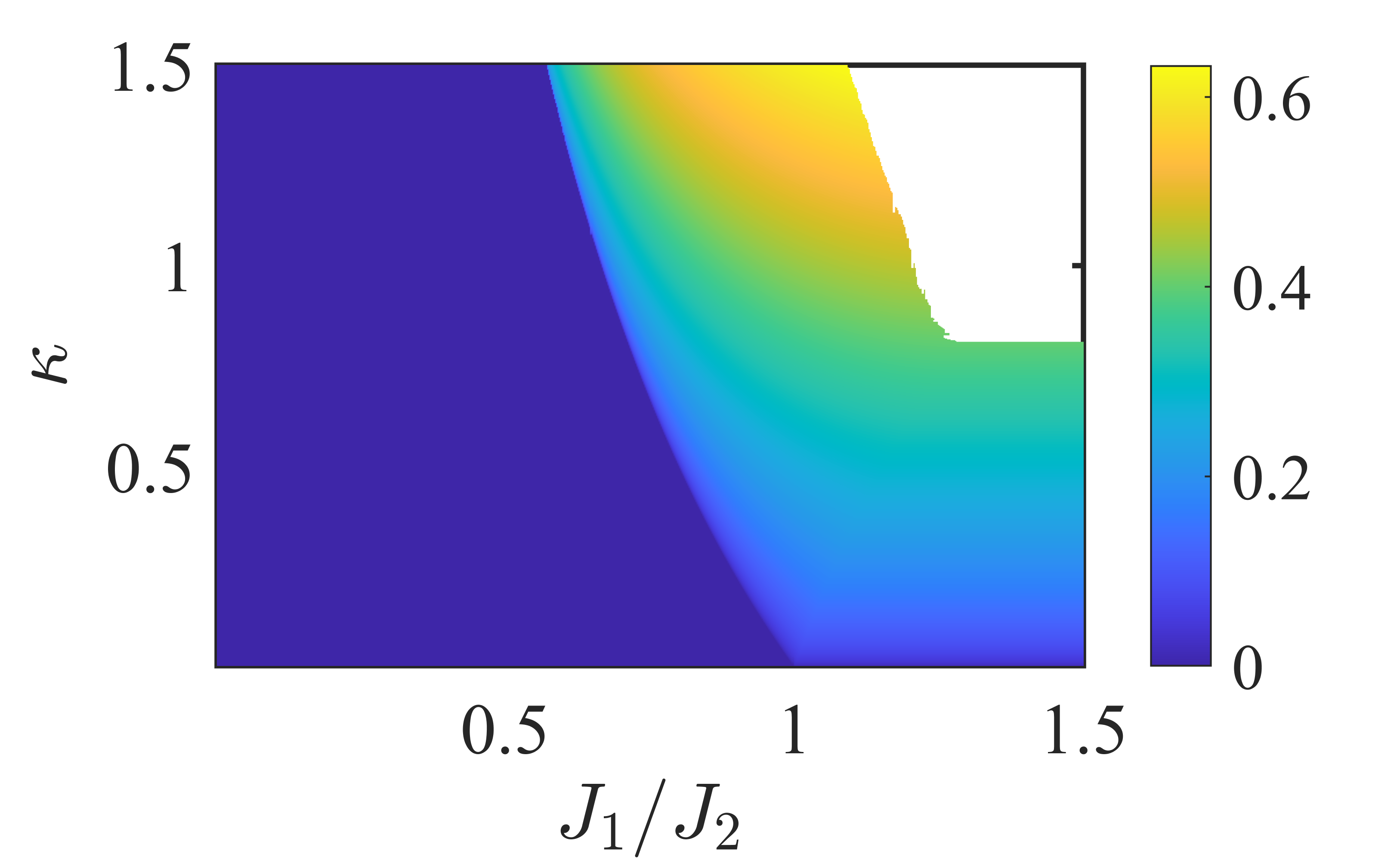
(a) $A_{1}$

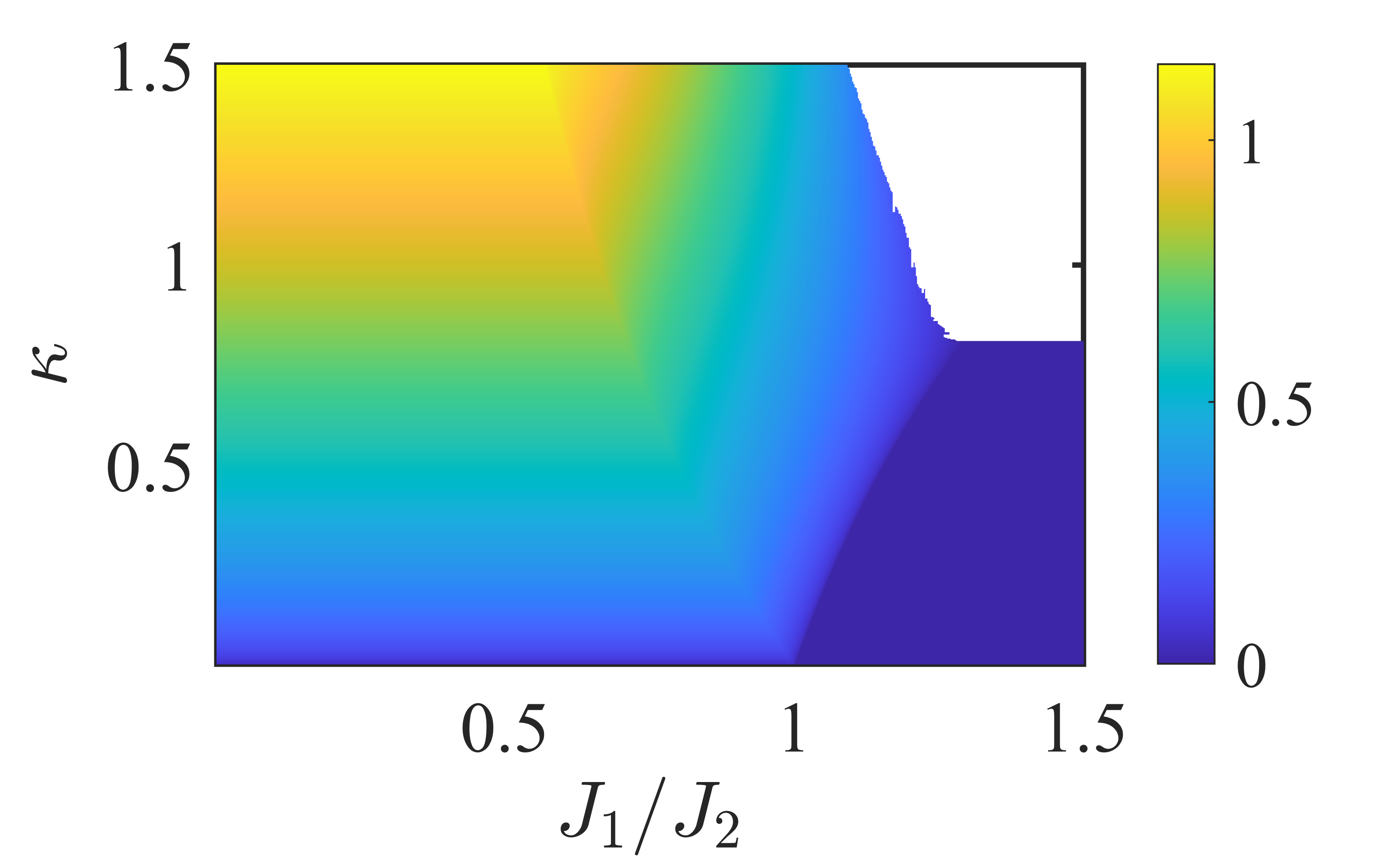
(b) $A_{2}$

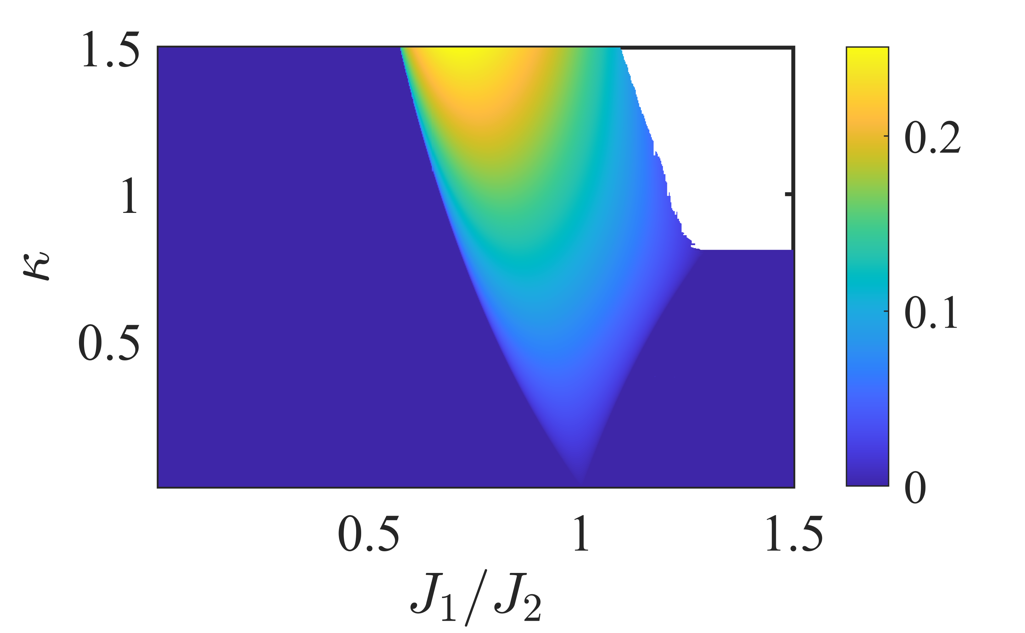
(c) $B_{1}$

Figure 15: The ansatz value (a) $A_{1}$, (b) $A_{2}$ and (c) $B_{1}$ of $(\pi,\pi)$-flux. $A_{1}$ is finite at $J_{1}$ is large and $A_{2}$ is large at $J_{1}$ is large. $B_{1}$ is finite only when $A_{1}$ and $A_{2}$ are both finite. $B_{2}$ is always zero in this condition.

With these ansatz values, the spinon dispersion and the structure factor can be obtained, which are shown in Fig. 16.

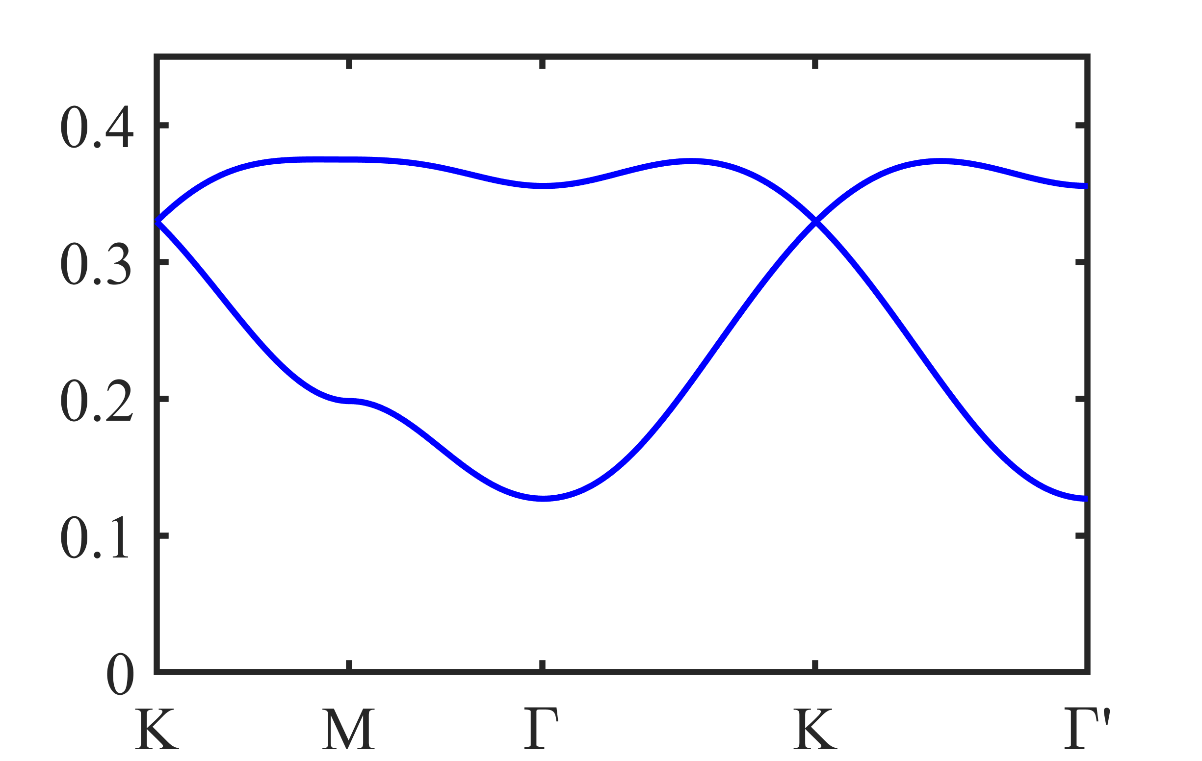
(a) Spinon dispersion

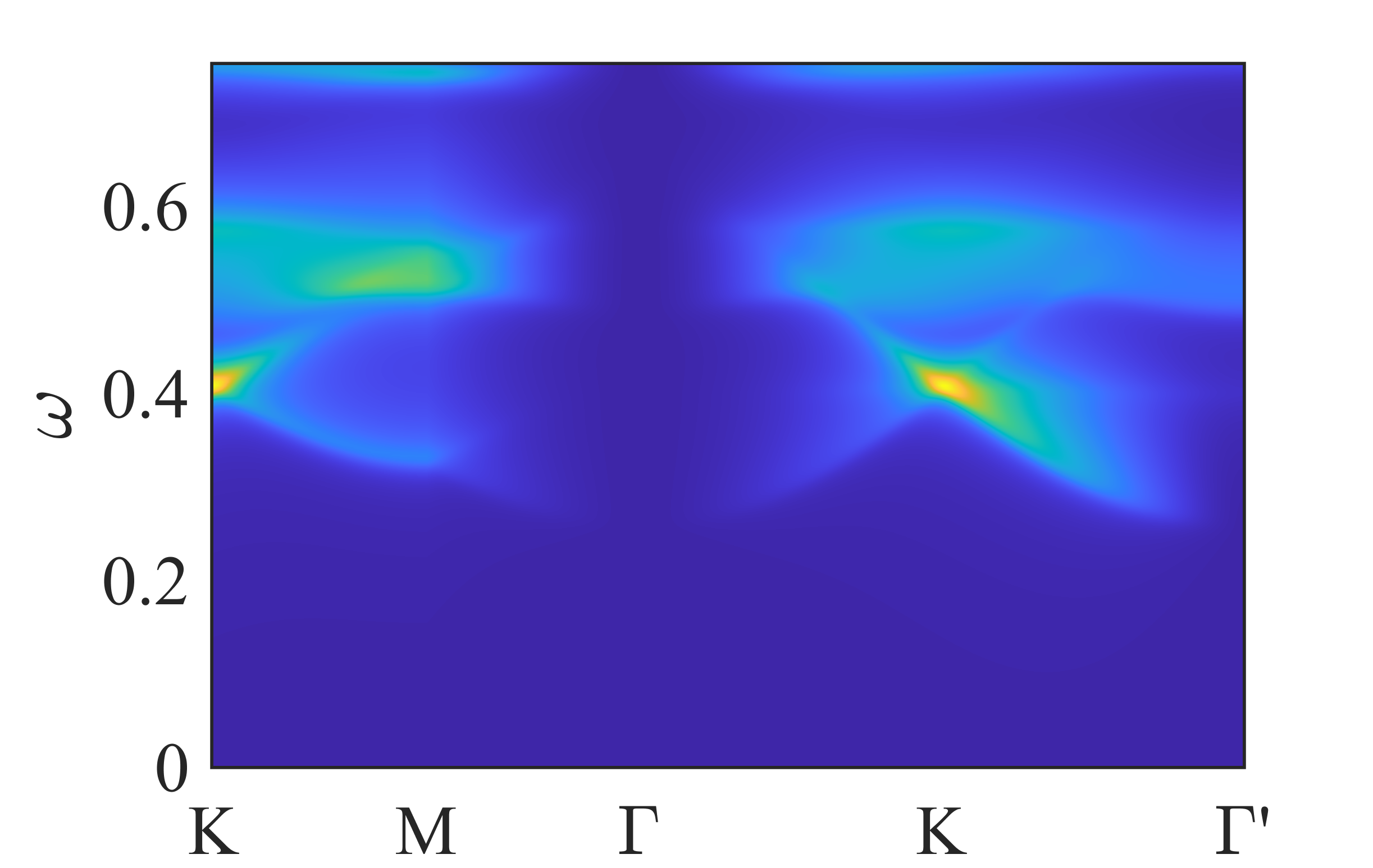
(b) dynamic structure factor

(c) static structure factor

Figure 16: (a) is the spinon dispersion, (b) is the dynamic structure factor, and (c) is the static structure factor of $(\pi,\pi)$-flux state ($J_{1}/J_{2}=0.7$). The plot path of (a) and (b) is shown in Fig. 1 (b) in Main Text.

As shown in Fig. 16 (a), the minima of the spinon dispersion is located at $\mathbf{Q}=(0,0)$, and magnetic order will form when $\kappa>\kappa_{c}$.

B.5 Plaquette-singlet states

First we consider the plaquette-singlet state in the empty square. The mean-field Hamiltonian can be written as

$$H_{\mathrm{MF}}=-N_{s}J_{1}\sum_{s}A_{1}\hat{A}_{s,s+1}+4N_{s}J_{1}\sum_{s}|A_{ij}|^{2}-4N_{s}\mu(\hat{n}-\kappa).$$ (158)

After Bogoliubov transformation, the mean-field Hamiltonian is diagonalized as

$$H_{\mathrm{MF}}=N_{s}\sum_{s}\omega_{s}(\gamma_{s\uparrow}^{\dagger}\gamma_{s\uparrow}+\gamma_{s\downarrow}^{\dagger}\gamma_{s\downarrow}+1)+N_{s}\left[\mu+\mu\kappa+4J_{1}\left|A_{1}\right|^{2}\right],$$ (159)

and the self-consistent equations are

$$8J_{1}A_{1} = -\sum_{s}\frac{\partial\omega_{s}}{\partial A_{1}},$$ (160)

$$1+\kappa = -\sum_{s}\frac{\partial\omega_{s}}{\partial\mu}.$$ (161)

The mean-field Hamiltonian and the self-consistent equations of the plaquette-singlet state in $J_{2}$-square is similar as the empty-square condition, except the existence of the $B_{2}$ in the $J_{2}$ bond. Solving the self-consistent equations, we get the ground state energies of these two plaquette-singlet states in physical condition $\kappa=1$, which is shown in Fig. 17.

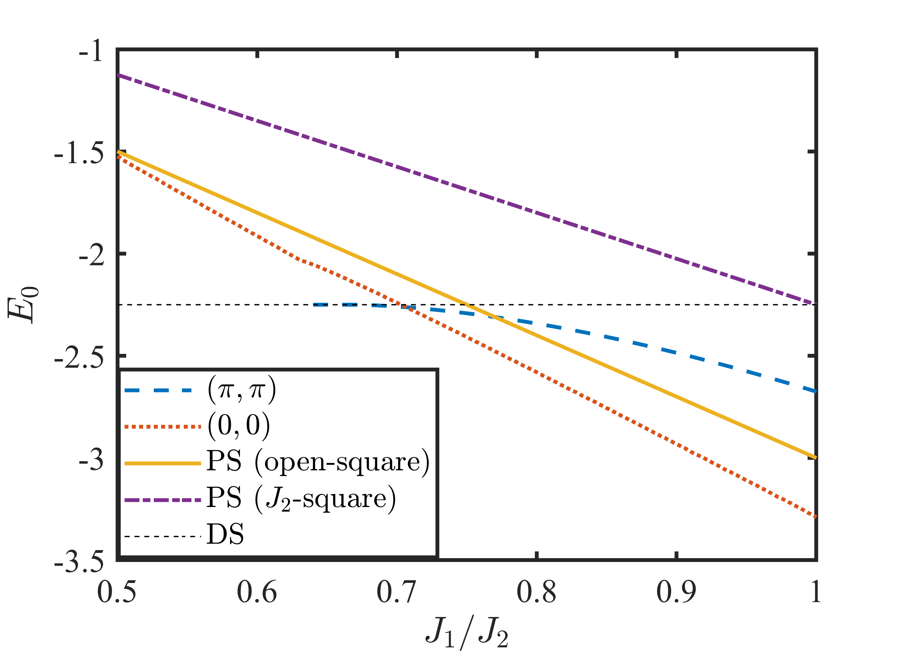
Figure 17: The mean-field ground state energies in the physical condition $\kappa=1$. The ground state energy of plaquette-singlet (PS) in the $J_{2}$-square is much larger than that in the empty-square condition because of the existence of $B_{2}$.

Appendix C Magnetic order from the zero-flux state

In the Schwinger boson formalism, the magnetic order is formed by the condensation of the Schwinger bosons. When the density of the boson is large than the critical $\kappa_{c}$, the dispersion of the spinon will become zero at several $\mathbf{Q}$ points, and the spinon will condense at these $\mathbf{Q}$ points and develop magnetic orders.

For the Shastry-Sutherland model, the Néel phase is formed by the condensation of the zero-flux ((0,0)-flux) state. As shown in Fig. 11 (a), the dispersion of spinon become zero at $\mathbf{Q}=(\pi,\pi)$. Note that $\mathbf{Q}=-\mathbf{Q}$. If we choose the empty square as the unit cell, after Fourier transformation $b_{\mathbf{r}}=\frac{1}{\sqrt{N_{s}}}\sum_{\mathbf{r}}e^{-i\mathbf{k}\cdot\mathbf{r}}b_{\mathbf{k}}$, the mean-field Hamiltonian becomes

$$H_{\mathrm{MF}}=\sum_{\mathbf{k}}\Psi_{\mathbf{k}}^{\dagger}D_{\mathbf{k}}\Psi_{\mathbf{k}}+N_{s}\left[\mu+\mu\kappa+8J_{1}\left|A_{1}\right|^{2}-2J_{2}\left|B_{2}\right|^{2}\right].$$ (162)

where we have used the Nambu spinor $\Psi_{\mathbf{k}}=(b_{0\mathbf{k}\uparrow},b_{1\mathbf{k}\uparrow},b_{2\mathbf{k}\uparrow},b_{3\mathbf{k}\uparrow},b_{0\mathbf{-k}\downarrow}^{\dagger},b_{1\mathbf{-k}\downarrow}^{\dagger},b_{2\mathbf{-k}\downarrow}^{\dagger},b_{3\mathbf{-k}\downarrow}^{\dagger})^{T}$. The subscript $s=0,1,2,3$ in $b_{s\bm{k}\sigma}$ is the atom index in the unit cell, which is shown in Fig. 6. The $8\times 8$ matrix $D_{\mathbf{k}}$ at $\mathbf{Q}$ is

$$D_{\mathbf{Q}} = \left(\begin{array}[]{cccccccc}-\mu&0&J_{2}B_{2}&0&0&J_{1}A_{1}&0&J_{1}A_{1}\\ 0&-\mu&0&J_{2}B_{2}&-J_{1}A_{1}&0&-J_{1}A_{1}&0\\ J_{2}B_{2}&0&-\mu&0&0&J_{1}A_{1}&0&J_{1}A_{1}\\ 0&J_{2}B_{2}&0&-\mu&-J_{1}A_{1}&0&-J_{1}A_{1}&0\\ 0&-J_{1}A_{1}&0&-J_{1}A_{1}&-\mu&0&J_{2}B_{2}&0\\ J_{1}A_{1}&0&J_{1}A_{1}&0&0&-\mu&0&J_{2}B_{2}\\ 0&-J_{1}A_{1}&0&-J_{1}A_{1}&J_{2}B_{2}&0&-\mu&0\\ J_{1}A_{1}&0&J_{1}A_{1}&0&0&J_{2}B_{2}&0&-\mu\end{array}\right),$$ (171)

In the critical density $\kappa_{c}$, it satisfies

$$-\mu+J_{2}B_{2}-2A_{1}=0.$$ (172)

At this point, $D_{\mathbf{Q}}$ has two eigenvectors with zero eigenvalue,

$$\Psi_{1} = \frac{1}{\sqrt{2}}\left(\begin{array}[]{cccccccc}0&1&0&1&1&0&1&0\end{array}\right)^{T},$$ (174)

$$\Psi_{2} = \frac{1}{\sqrt{2}}\left(\begin{array}[]{cccccccc}-1&0&-1&0&0&1&0&1\end{array}\right)^{T}.$$ (176)

Therefore, the condensation at $\mathbf{Q}$ is $\langle\Psi_{\mathbf{Q}}\rangle=c_{1}\Psi_{1}+c_{2}\Psi_{2}$, where $c_{1,2}$ are two complex numbers. We define $x_{s}\equiv(\langle b_{(X,Y,s)\uparrow}\rangle,\langle b_{(X,Y,s)\downarrow}\rangle)^{T}$, then condensation on site $(X,Y,s)$ is given by

$$x_{0} = x_{2}=\frac{(-1)^{X+Y}}{\sqrt{2}}\left(\begin{array}[]{c}-c_{2}\\ c_{1}^{*}\end{array}\right),$$ (179)

$$x_{1} = x_{3}=\frac{(-1)^{X+Y}}{\sqrt{2}}\left(\begin{array}[]{c}c_{1}\\ c_{2}^{*}\end{array}\right),$$ (182)

and the ordered magnetic momentum is then $\mathbf{S}(X,Y,s)=\frac{1}{2}x_{s}^{\dagger}\bm{\sigma}x_{s}$. Thus we have

$$\mathbf{S}(X,Y,0) = \mathbf{S}(X,Y,2)=\mathbf{n},$$ (183)

$$\mathbf{S}(X,Y,1) = \mathbf{S}(X,Y,3)=-\mathbf{n},$$ (184)

where $\mathbf{n}$ is the $SO(3)$ vector corresponded with the $SU(2)$ vector $(-c_{2},c_{1}^{*})^{T}$. This gives the Néel magnetic order momentum,

$$\mathbf{S}(\mathbf{r}) = (-1)^{\mathbf{r}}\mathbf{n}.$$ (185)

Appendix D Magnetic order from the $\pi$-flux state

In the large $\kappa$ limit, the spinon in the $\pi$-flux spin liquid phase will also condense and form magnetic order. In this section, we discuss the magnetic order from the $\pi$-flux state.

The mean-field Hamiltonian of $(\pi,\pi)$-flux state is

$$H_{\mathrm{MF}}=\sum_{\mathbf{k}}\Psi_{\mathbf{k}}^{\dagger}D_{\mathbf{k}}\Psi_{\mathbf{k}}+N_{s}\left[\mu+\mu\kappa+8J_{1}(\left|A_{1}\right|^{2}-\left|B_{1}\right|^{2})+2J_{2}\left|A_{2}\right|^{2}\right],$$ (186)

where the expression $D_{\mathbf{k}}$ is shown in Eq. (142).

For simplicity, we only discuss the large $J_{1}$ condition, where only $A_{1}$ is finite. In the mean-field level, the Shastry-Sutherland lattice is equivalent to the square lattice in this condition where $A_{2}$ and $B_{2}$ vanishes. The magnetic order of this condition is

$$\mathbf{S}(X,Y,0) = \mathbf{n}_{1}+\mathbf{n}_{2}+\mathbf{n}_{3},$$ (187)

$$\mathbf{S}(X,Y,1) = -\mathbf{n}_{1}+\mathbf{n}_{2}-\mathbf{n}_{3},$$ (188)

$$\mathbf{S}(X,Y,2) = -\mathbf{n}_{1}-\mathbf{n}_{2}+\mathbf{n}_{3},$$ (189)

$$\mathbf{S}(X,Y,3) = \mathbf{n}_{1}-\mathbf{n}_{2}-\mathbf{n}_{3},$$ (190)

which is discussed in Ref. [36], and $n_{1}^{2}+n_{2}^{2}+n_{3}^{2}=n^{2}$. The details of the calculation can be referred to Appendix C in Ref. [36].

Appendix E Self-consistent spin wave theory

In this section, we introduce the self-consistent spin wave theory in details. Near the phase boundary of the Néel phase, the quantum fluctuation is significant and the interaction of magnons takes important role. For the Shastry-Sutherland model, the linear spin wave Hamiltonian is not positive or semi-positive definite in $J_{1}/J_{2}<1$, and the linear spin wave theory breaks down in this region. The nonlinear spin wave theory also breaks down because the correction of magnon interaction depends on the magnon wave function of linear spin wave theory. Therefore, we need to use a self-consistent spin wave theory to study Néel phase of the Shastry-Sutherland model in $J_{1}/J_{2}<1$.

Spin wave theory is to describe the ordered phase in terms of small fluctuations of the spins about their expectation values, which can be regarded as the classical ground state of the Hamiltonian. For the Shastry-Sutherland model, the magnetic ordered state is a Néel state, and the classical ground state is the Néel antiferromagnetic state. With the classical ground state, the spin Hamiltonian can be expressed by the boson operators by the Holstein-Primakoff transformation[43]. Expanding the Hamiltonian by $1/S$ as we regarding $S$ as a large number, the Hamiltonian is transformed to

$$H=H_{0}+H_{2}+H_{4}+H_{6}+\dots,$$ (191)

where linear term $H_{1}$ vanishes if the classical ground state is proper. Keeping up to quadratic terms $H_{2}$, one obtains the noninteracting spin wave Hamiltonian. The higher order terms $H_{4}+H_{6}+\dots$ introduce the interactions of magnons. For the Shastry-Sutherland model, if we choose the “$J_{2}$-square” as the unit cell, the linear spin wave Hamiltonian $H_{2}$ in the momentum space can be written as

$$H_{2} = \sum_{\bm{k}}\left(\begin{array}[]{llllllll}a_{\bm{k}}^{\dagger}&b_{\bm{k}}^{\dagger}&c_{\bm{k}}^{\dagger}&d_{\bm{k}}^{\dagger}&a_{-\bm{k}}&b_{-\bm{k}}&c_{-\bm{k}}&d_{-\bm{k}}\end{array}\right)\mathcal{H}_{\bm{k}}\left(\begin{array}[]{c}a_{\bm{k}}\\ b_{\bm{k}}\\ c_{\bm{k}}\\ d_{\bm{k}}\\ a_{-\bm{k}}^{\dagger}\\ b_{-\bm{k}}^{\dagger}\\ c_{-\bm{k}}^{\dagger}\\ d_{-\bm{k}}^{\dagger}\end{array}\right),$$ (201)

here $a,b,c,d$ are the Holstein-Primakoff bosons for the unit cell has 4 sites. The $\mathcal{H}_{\bm{k}}$ satisfies

$$\mathcal{H}_{\bm{k}} = \left(\begin{array}[]{cc}\boldsymbol{B}_{\bm{k}}&\boldsymbol{A}_{\bm{k}}\\ \boldsymbol{A}_{\bm{k}}^{\dagger}&\boldsymbol{B}_{-\bm{k}}^{T}\end{array}\right),$$ (204)

$$\boldsymbol{A}_{\bm{k}} = \left(\begin{array}[]{cccccccc}0&\frac{1}{2}J_{1}(1+\mathrm{e}^{ik_{1}})&0&\frac{1}{2}J_{1}(1+\mathrm{e}^{ik_{2}})\\ \frac{1}{2}J_{1}(1+\mathrm{e}^{-ik_{1}})&0&\frac{1}{2}J_{1}(1+\mathrm{e}^{ik_{2}})&0\\ 0&\frac{1}{2}J_{1}(1+\mathrm{e}^{-ik_{2}})&0&\frac{1}{2}J_{1}(1+\mathrm{e}^{-ik_{1}})\\ \frac{1}{2}J_{1}(1+\mathrm{e}^{-ik_{2}})&0&\frac{1}{2}J_{1}(1+\mathrm{e}^{ik_{1}})&0\end{array}\right),$$ (209)

$$\boldsymbol{B}_{\bm{k}} = \left(\begin{array}[]{cccc}2J_{1}-\frac{1}{2}J_{2}&0&0&0\\ 0&2J_{1}-\frac{1}{2}J_{2}&0&\frac{1}{2}J_{2}\mathrm{e}^{i(k_{1}-k2)}\\ 0&0&2J_{1}-\frac{1}{2}J_{2}&0\\ 0&\frac{1}{2}J_{2}\mathrm{e}^{i(-k_{1}+k2)}&0&2J_{1}-\frac{1}{2}J_{2}\\ \end{array}\right).$$ (214)

Using Bogoliubov transformation to diagonalize the $\mathcal{H}_{\bm{k}}$, we will get the linear spin wave dispersion and wave functions, which breaks down at $J_{1}/J_{2}<1$. The self-consistent spin wave theory is to use the boson-pair expectation values to decouple the quartic terms. We use a specific term for example:

$$\sum_{\bm{k},\bm{p},\bm{q}}V(\bm{k},\bm{p},\bm{q})a_{\bm{k}}^{\dagger}b_{\bm{p}}^{\dagger}a_{\bm{q}}b_{\bm{k}+\bm{p}-\bm{q}}$$ (215)

$$\approx \sum_{\bm{k}}\left[\sum_{\bm{p},\bm{q}}V(\bm{k},\bm{p},\bm{k})\langle b_{\bm{p}}^{\dagger}b_{\bm{p}}\rangle\right]a_{\bm{k}}^{\dagger}a_{\bm{k}}+\dots$$

$$= \sum_{\bm{k}}f(\bm{k})a_{\bm{k}}^{\dagger}a_{\bm{k}}+\dots.$$

Here $a$ and $b$ are the boson operators of different flavors, and we set $\sum_{\bm{k}}f(\bm{k})\equiv\sum_{\bm{p},\bm{q}}V(\bm{k},\bm{p},\bm{k})\langle b_{\bm{p}}^{\dagger}b_{\bm{p}}\rangle$. The symbol $(\dots)$ represents the other decoupling types. Therefore, the Hamiltonian is transformed into

$$H = H_{2}+H_{4}+\dots$$ (216)

$$= H_{2}+\widetilde{H}_{2}+H_{4}-\widetilde{H}_{2}+\dots$$

$$= H_{2}^{\prime}+H_{4}^{\prime},$$

and $H_{4}^{\prime}=0$ in the mean-field level. We call this theory a self-consistent spin wave theory because the decoupled quartic term $\widetilde{H}_{2}$ need to be calcultaed self-consistently. The effects of magnon interaction is considered in this theory. When $H_{2}$ is not positive or semi-positive definite, this method may also work because we only need to keep $H_{2}^{\prime}$ to be positive and semi-positive definite. For the Shastry-Sutherland model, the self-consistent spin wave theory works in the $J_{1}/J_{2}>0.65$, where the magnetic order parameter vanishes, which indicates the phase boundary of the Néel state.

Appendix F Continuum limit of linear spin wave on Shastry-Sutherland model

In this section, we follow the prescription in Refs. [44] to derive the continuum field theory of the linear spin wave on Shastry-Sutherland model. The magnon velocity can be obtained from this continuum field theory.

We assume the Néel order is along the $z$ direction

$$\langle\bm{S}_{i}\rangle=(-1)^{s}S\hat{\bm{z}},$$ (217)

here $s=0,1,2,3$, which is the sublattice label shown in Fig. 6. The lattice vectors are $2\hat{\bm{x}}$ and $2\hat{\bm{y}}$. The site position in the Shastry-Sutherland lattice is expressed by $(\bm{r},s)$, where $\bm{r}$ is the unit cell position and $s$ is the sublattice label. After Holstein-Primakoff transformation, the linear spin wave Hamiltonian is

$$H_{LSW}=S\sum_{\bm{r}} \left\{(4J_{1}-J_{2})\sum_{s}b_{s\bm{r}}^{\dagger}b_{s\bm{r}}+J_{2}\left(b_{1\bm{r}}^{\dagger}b_{3\bm{r}+\hat{\bm{x}}+\hat{\bm{y}}}+b_{0\bm{r}}^{\dagger}b_{2\bm{r}+\hat{\bm{x}}-\hat{\bm{y}}}+\mathrm{h.c.}\right)\right.$$ (218)

$$\left.-J_{1}\left[b_{0\bm{r}}\left(b_{1\bm{r}+\hat{\bm{x}}}+b_{1\bm{r}-\hat{\bm{x}}}+b_{3\bm{r}+\hat{\bm{y}}}+b_{3\bm{r}-\hat{\bm{y}}}\right)+b_{2\bm{r}}\left(b_{1\bm{r}+\hat{\bm{y}}}+b_{1\bm{r}-\hat{\bm{y}}}+b_{3\bm{r}+\hat{\bm{x}}}+b_{3\bm{r}-\hat{\bm{x}}}\right)+\mathrm{h.c.}\right]\right\}.$$

In the imaginary time path integral formalism, the bosonic $b_{s\bm{r}}$ operators become complex fields. For later convenience, the operators are transformed to complex fields as

$$b_{0\bm{r}} \rightarrow \phi_{0}(\bm{r}),$$ (219)

$$b_{1\bm{r}} \rightarrow \phi_{1}^{*}(\bm{r}),$$ (220)

$$b_{2\bm{r}} \rightarrow \phi_{2}(\bm{r}),$$ (221)

$$b_{3\bm{r}} \rightarrow \phi_{3}^{*}(\bm{r}).$$ (222)

The gradient expansion is used to get the continuum field theory from the linear spin wave Hamiltonian in Eq. (218),

$$\phi^{*}_{s}(\bm{r})\phi_{s^{\prime}}(\bm{r}+\bm{a})=\phi_{s}^{*}(\bm{r})\left[\phi_{s^{\prime}}(\bm{r})+\bm{a}\cdot\nabla_{\bm{r}}\phi_{s^{\prime}}(\bm{r})+\frac{1}{2}(\bm{a}\cdot\nabla_{\bm{r}})^{2}\phi_{s^{\prime}}(\bm{r})+\dots\right].$$ (223)

Substituting the gradient expansion to the linear spin wave Hamiltonian and keep up to the 2nd order, we obtains the Hamiltonian density,

$$\mathcal{H}=\mathcal{H}_{0}+\mathcal{H}_{1}+\mathcal{H}_{2},$$ (224)

here $\mathcal{H}_{0}$ has no gradient, $\mathcal{H}_{0}$ has the 1nd order gradient terms and $\mathcal{H}_{2}$ has the 2st order gradient terms. The expression of $\mathcal{H}_{0}$ is

$$\mathcal{H}_{0}=\left(\begin{array}[]{llll}\phi_{0}^{*}(\bm{r})&\phi_{1}^{*}(\bm{r})&\phi_{2}^{*}(\bm{r})&\phi_{3}^{*}(\bm{r})\end{array}\right)\left(\begin{array}[]{cccc}4J_{1}-J_{2}&-2J_{1}&J_{2}&-2J_{1}\\ -2J_{1}&4J_{1}-J_{2}&-2J_{1}&J_{2}\\ J_{2}&-2J_{1}&4J_{1}-J_{2}&-2J_{1}\\ -2J_{1}&J_{2}&-2J_{1}&4J_{1}-J_{2}\end{array}\right)\left(\begin{array}[]{c}\phi_{0}(\bm{r})\\ \phi_{1}(\bm{r})\\ \phi_{2}(\bm{r})\\ \phi_{3}(\bm{r})\end{array}\right),$$ (234)

and the eigenvalues and eigenvectors of $\mathcal{H}_{0}$ are

$$0,\Psi_{0}=\left(\begin{array}[]{c}1/2\\ 1/2\\ 1/2\\ 1/2\end{array}\right);\ 8J_{1}S,\Psi_{1}=\left(\begin{array}[]{c}1/2\\ -1/2\\ 1/2\\ -1/2\end{array}\right);\ (4J1-2J_{2})S,\Psi_{2}=\left(\begin{array}[]{c}1/2\\ 1/2\\ -1/2\\ -1/2\end{array}\right);\ (4J1-2J_{2})S,\Psi_{3}=\left(\begin{array}[]{c}1/2\\ -1/2\\ -1/2\\ 1/2\end{array}\right);$$ (251)

The eigenvector $\Psi_{0}$ with zero eigenvalue is the Goldstone mode. Then the $\mathcal{H}_{0}$ is diagonalized as

$$\mathcal{H}_{0}=8SJ_{1}\Psi_{1}^{*}\Psi_{1}+S(4J_{1}-2J_{2})(\Psi_{2}^{*}\Psi_{2}+\Psi_{3}^{*}\Psi_{3}).$$ (252)

For later convenience, we set $\bm{\phi}\equiv\left(\begin{array}[]{llll}\phi_{0}(\bm{r})&\phi_{1}(\bm{r})&\phi_{2}(\bm{r})&\phi_{3}(\bm{r})\end{array}\right)^{T}$ and $\bm{\Psi}\equiv\left(\begin{array}[]{llll}\Psi_{0}(\bm{r})&\Psi_{1}(\bm{r})&\Psi_{2}(\bm{r})&\Psi_{3}(\bm{r})\end{array}\right)^{T}$. The expression of $\mathcal{H}_{1}$ is

$$\mathcal{H}_{1} = SJ_{2}[\phi_{1}(\partial_{x}+\partial_{y})\phi_{3}^{*}+\phi_{0}^{*}(\partial_{x}-\partial_{y})\phi_{2}-\phi_{3}(\partial_{x}+\partial_{y})\phi_{1}^{*}-\phi_{2}^{*}(\partial_{x}-\partial_{y})\phi_{0}]$$ (261)

$$= SJ_{2}\left[\bm{\phi}^{*}\left(\begin{array}[]{cccc}0&0&1&0\\ 0&0&0&1\\ -1&0&0&0\\ 0&-1&0&0\end{array}\right)\partial_{x}\bm{\phi}+\bm{\phi}^{*}\left(\begin{array}[]{cccc}0&0&-1&0\\ 0&0&0&1\\ 1&0&0&0\\ 0&-1&0&0\end{array}\right)\partial_{y}\bm{\phi}\right]$$

$$= SJ_{2}\left[\bm{\Psi}^{*}\left(\begin{array}[]{cccc}0&0&-1&0\\ 0&0&0&-1\\ 1&0&0&0\\ 0&1&0&0\end{array}\right)\partial_{x}\bm{\Psi}+\bm{\Psi}^{*}\left(\begin{array}[]{cccc}0&0&0&-1\\ 0&0&-1&0\\ 0&1&0&0\\ 1&0&0&0\end{array}\right)\partial_{y}\bm{\Psi}\right].$$ (270)

Now we consider the 2nd order gradient terms $\mathcal{H}_{2}$, whose expression is

$$\mathcal{H}_{2}= \frac{1}{2}SJ_{2}[\phi_{1}(\partial_{x}+\partial_{y})^{2}\phi_{3}^{*}+\phi_{0}(\partial_{x}-\partial_{y})^{2}\phi_{2}^{*}+\phi_{3}(\partial_{x}+\partial_{y})^{2}\phi_{1}^{*}+\phi_{2}(\partial_{x}-\partial_{y})^{2}\phi_{0}^{*}]$$ (271)

$$-SJ_{1}[\phi_{0}(\partial_{x}^{2}\phi_{1}^{*}+\partial_{y}^{2}\phi_{3}^{*})+\phi_{2}(\partial_{y}^{2}\phi_{1}^{*}+\partial_{x}^{2}\phi_{3}^{*})+\mathrm{c.c.}].$$

In the continuum limit, the low energy effective theory is only contributed by the Goldstone mode $\Psi_{0}$. Therefore, we need to integrate the high energy modes $\Psi_{1},\Psi_{2}$ and $\Psi_{3}$ to get the effective field theory of $\Psi_{0}$. For this purpose, we only keep the $\Psi_{0}^{*}(\dots)\Psi_{0}$ terms in $\mathcal{H}_{2}$ because the other terms in $\mathcal{H}_{2}$ do not contribute the effective field theory of $\Psi_{0}$ up to 2nd order gradient terms. Then we just need to replace $\phi_{s}$ by $\frac{1}{2}\Psi_{0}$,

$$\mathcal{H}_{2} \cong \frac{1}{4}SJ_{2}[\Psi_{0}(\partial_{x}+\partial_{y})^{2}\Psi_{0}^{*}+\Psi_{0}(\partial_{x}-\partial_{y})^{2}\Psi_{0}^{*}]-\frac{1}{2}SJ_{1}[\Psi_{0}(\partial_{x}^{2}+\partial_{y}^{2})\Psi_{0}^{*}+\Psi_{0}^{*}(\partial_{x}^{2}+\partial_{y}^{2})\Psi_{0}]+\dots$$ (272)

$$= S(J_{1}-\frac{1}{2}J_{2})\left[(\partial_{x}\Psi_{0}^{*})(\partial_{x}\Psi_{0})+(\partial_{y}\Psi_{0}^{*})(\partial_{y}\Psi_{0})\right].$$

The Lagrangian density of the linear spin wave theory is

$$\mathcal{L} = \phi_{0}^{*}\partial_{\tau}\phi_{0}-\phi_{1}^{*}\partial_{\tau}\phi_{1}+\phi_{2}^{*}\partial_{\tau}\phi_{2}-\phi_{3}^{*}\partial_{\tau}\phi_{3}-\mathcal{H}$$ (273)

$$= \Psi_{0}^{*}\partial_{\tau}\Psi_{1}+\Psi_{1}^{*}\partial_{\tau}\Psi_{0}+\Psi_{2}^{*}\partial_{\tau}\Psi_{3}+\Psi_{3}^{*}\partial_{\tau}\Psi_{2}-\mathcal{H}.$$

By integrating the high energy modes by Gaussian part of their action in $\mathcal{H}$, we get the effective action for $\Psi_{0}$, whose Lagrangian density is

$$\mathcal{L}_{\mathrm{eff}}=\frac{1}{8SJ_{1}}(\partial_{\tau}\Psi_{0}^{*})(\partial_{\tau}\Psi_{0})+S\left[J_{1}-\frac{J_{2}}{2}-\frac{J_{2}^{2}}{4J_{1}-2J_{2}}\right]\left[(\partial_{x}\Psi_{0}^{*})(\partial_{x}\Psi_{0})+(\partial_{y}\Psi_{0}^{*})(\partial_{y}\Psi_{0})\right],$$ (274)

which yields the dispersion relation

$$\frac{1}{8SJ_{1}}\omega^{2}=S\left[J_{1}-\frac{J_{2}}{2}-\frac{J_{2}^{2}}{4J_{1}-2J_{2}}\right]\bm{k}^{2}.$$ (275)

Finally, we get the magnon velocity $v_{\mathrm{sw}}$ of linear spin wave theory,

$$v_{\mathrm{sw}}=4SJ_{1}\sqrt{\frac{J_{1}-J_{2}}{2J_{1}-J_{2}}},$$ (276)

which vanishes at $J_{1}=J_{2}$, where the linear spin wave theory breaks down. For the magnon velocity of the self-consistent spin wave theory, it can only be calculated numerically. The magnon velocities and magnetic moment sizes calculated by self-consistent and linear spin wave theory are shown in Table 1.

$J_{1}/J_{2}$	0.7	0.75	0.8	0.85	0.9	0.95	1	1.05	1.1	1.15	1.2	1.25	1.13	1.35	1.4
$v_{\mathrm{SCSW}}$	0.470	0.585	0.695	0.802	0.905	1.005	1.103	1.199	1.294	1.387	1.478	1.569	1.659	1.748	1.836
$v_{\mathrm{LSW}}$	n.a.	n.a.	n.a.	n.a.	n.a.	n.a.	0	0.447	0.635	0.781	0.907	1.021	1.126	1.225	1.320
$m_{\mathrm{SCSW}}$	0.032	0.069	0.096	0.116	0.130	0.143	0.153	0.160	0.166	0.171	0.176	0.180	0.183	0.186	0.188
$m_{\mathrm{LSW}}$	n.a.	n.a.	n.a.	n.a.	n.a.	n.a.	n.a.	n.a.	0.067	0.109	0.136	0.156	0.171	0.183	0.193

Table 1: Magnon velocities and magnetic moment sizes from self-consistent spin wave(SCSW) and linear spin wave(LSW). The unit of the velocities is $J_{2}a$, where $a$ is the square lattice constant. The magnetic moment is calculated by $1/2-\langle n_{m}\rangle$, here $\langle n_{m}\rangle$ is the average magnon density. “n.a.” means not applicable.

Appendix G Exact diagonalization of 32-site Shastry-Sutherland model

We study the ground state properties of the Shastry-Sutherland model [see Eq. (1) in Main Text] by exact diagonalization, on finite-size($2\sqrt{2}\times 2\sqrt{2}\times 4$) lattice with $32$ sites (see Fig. 18). With periodic boundary conditions this preserves the full lattice symmetries of the Shastry-Sutherland model.

The ground state energies and wave functions are obtained by the Lanczos method. The following lattice symmetries are exploited to reduce the Hilbert space sizes, (a) lattice translations (with respect to 4-site unit cell); (b) four-fold rotation $C_{4}$ around the center of an empty square, in the translation trivial sector. The ground states are found in the sector with trivial translations and $C_{4}$ eigenvalue $(+1)$. The reduced Hilbert space sizes is $18788230$ for this $32$-site lattice.

We consider antiferromagntic $J_{1}$ and $J_{2}$ couplings and set $J_{2}=1$. The ground state energy and some of the ground state spin-spin correlation functions are shown in Fig. 4 in Main Text. We note that for $J_{1}/J_{2}\leq 0.67578125$ the exact ground state is the dimer-singlet state, and a level crossing happens for $J_{1}/J_{2}$ between $0.67578125$ and $0.677734375$. This level crossing point is consistent with previous exact diagonalization studies [45]

Here we also present the ground state expectation values of the 4-site ring exchange operators around “$J_{2}$ square” and “empty square” from the exact diagonalization, and compare them to the Schwinger boson mean-field theory results (see Fig. 19). This operator cyclically permutes spins on the four sites involved, namely it is $\sum_{\{s_{i}\}}(|s_{1},s_{2},s_{3},s_{4}\rangle\langle s_{2},s_{3},s_{4},s_{1}|+\text{h.c.})$.

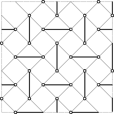
Figure 18: The $32$-site Shastry-Sutherland lattice used in the ED study. Open circles indicate distinct sites under periodic boundary condition. $J_{2}$ and $J_{1}$ bonds are depicted as thick and thin solid lines respectively.

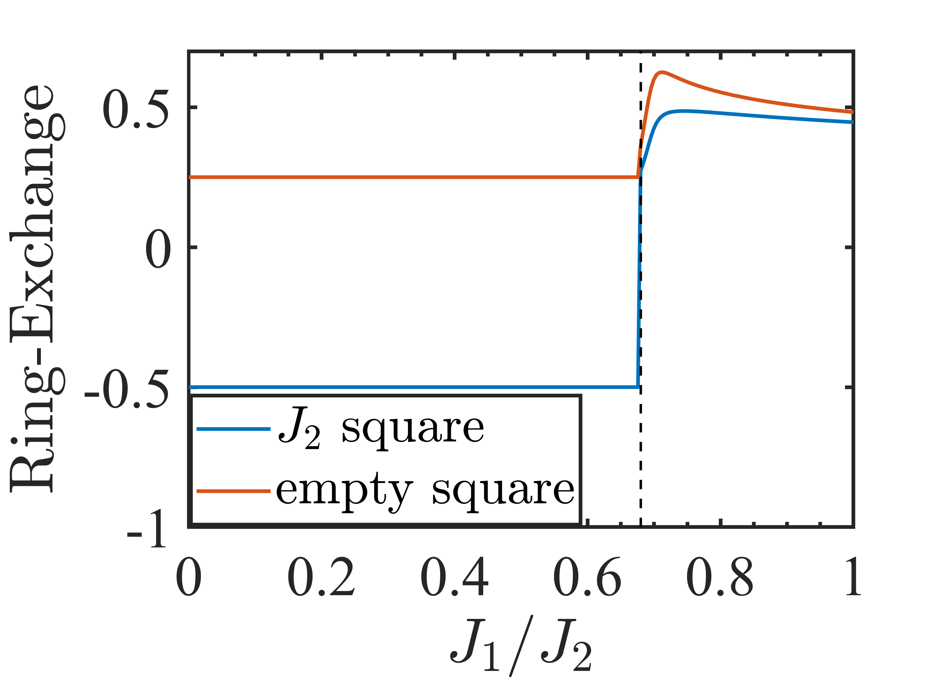
(a) Exact diagonalization

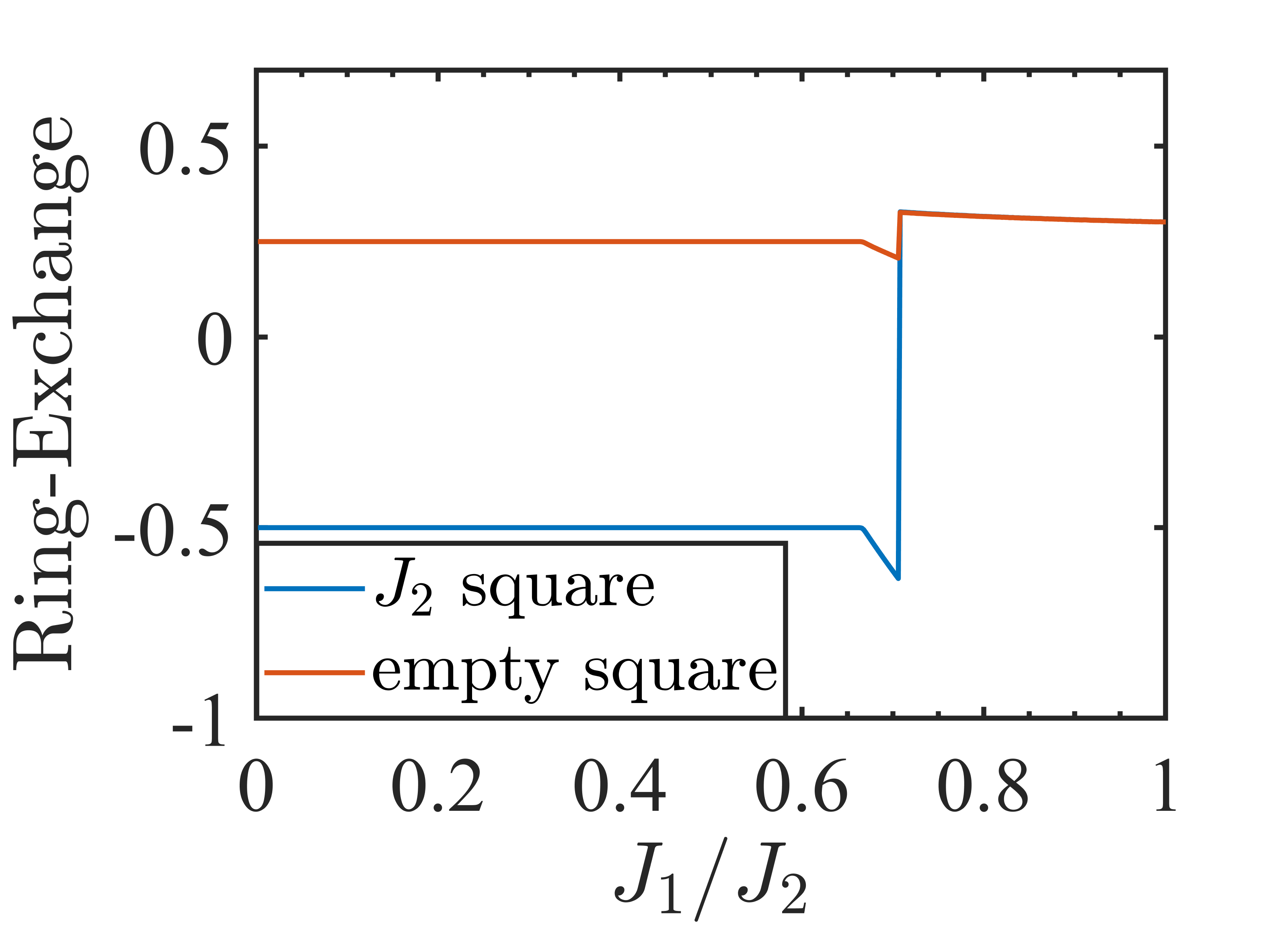
(b) Schwinger boson mean field theory

Figure 19: Expectation values of 4-site ring exchange operators around “$J_{2}$ square” and “empty square” calculated by (a) exact diagonalization and (b) Schwinger boson mean field theory.

References

- Cui et al. [2023] Y. Cui, L. Liu, H. Lin, K.-H. Wu, W. Hong, X. Liu, C. Li, Z. Hu, N. Xi, S. Li, R. Yu, A. W. Sandvik, and W. Yu, Proximate deconfined quantum critical point in , Science 380, 1179 (2023), https://www.science.org/doi/pdf/10.1126/science.adc9487 .
- Zayed et al. [2017] M. E. Zayed, C. Rüegg, J. Larrea J., A. M. Läuchli, C. Panagopoulos, S. S. Saxena, M. Ellerby, D. F. McMorrow, T. Strässle, S. Klotz, G. Hamel, R. A. Sadykov, V. Pomjakushin, M. Boehm, M. Jiménez-Ruiz, A. Schneidewind, E. Pomjakushina, M. Stingaciu, K. Conder, and H. M. Rønnow, 4-spin plaquette singlet state in the shastry–sutherland compound srcu2(bo3)2, Nature Physics 13, 962 (2017).
- Guo et al. [2020] J. Guo, G. Sun, B. Zhao, L. Wang, W. Hong, V. A. Sidorov, N. Ma, Q. Wu, S. Li, Z. Y. Meng, A. W. Sandvik, and L. Sun, Quantum phases of from high-pressure thermodynamics, Phys. Rev. Lett. 124, 206602 (2020).
- Jiménez et al. [2021] J. L. Jiménez, S. P. G. Crone, E. Fogh, M. E. Zayed, R. Lortz, E. Pomjakushina, K. Conder, A. M. Läuchli, L. Weber, S. Wessel, A. Honecker, B. Normand, C. Rüegg, P. Corboz, H. M. Rønnow, and F. Mila, A quantum magnetic analogue to the critical point of water, Nature 592, 370 (2021).
- Senthil et al. [2004] T. Senthil, A. Vishwanath, L. Balents, S. Sachdev, and M. P. A. Fisher, Deconfined quantum critical points, Science 303, 1490 (2004), https://www.science.org/doi/pdf/10.1126/science.1091806 .
- Sachdev [2008] S. Sachdev, Quantum magnetism and criticality, Nature Physics 4, 173 (2008).
- Sandvik [2007] A. W. Sandvik, Evidence for deconfined quantum criticality in a two-dimensional heisenberg model with four-spin interactions, Phys. Rev. Lett. 98, 227202 (2007).
- Xi et al. [2023] N. Xi, H. Chen, Z. Y. Xie, and R. Yu, Plaquette valence bond solid to antiferromagnet transition and deconfined quantum critical point of the shastry-sutherland model, Phys. Rev. B 107, L220408 (2023).
- Balents [2010] L. Balents, Spin liquids in frustrated magnets, Nature 464, 199 (2010).
- Sriram Shastry and Sutherland [1981] B. Sriram Shastry and B. Sutherland, Exact ground state of a quantum mechanical antiferromagnet, Physica B+C 108, 1069 (1981).
- Nakano and Sakai [2018] H. Nakano and T. Sakai, Third boundary of the shastry–sutherland model by numerical diagonalization, Journal of the Physical Society of Japan 87, 123702 (2018), https://doi.org/10.7566/JPSJ.87.123702 .
- Koga and Kawakami [2000] A. Koga and N. Kawakami, Quantum phase transitions in the shastry-sutherland model for , Phys. Rev. Lett. 84, 4461 (2000).
- Zhao et al. [2019] B. Zhao, P. Weinberg, and A. W. Sandvik, Symmetry-enhanced discontinuous phase transition in a two-dimensional quantum magnet, Nature Physics 15, 678 (2019).
- Corboz and Mila [2013] P. Corboz and F. Mila, Tensor network study of the shastry-sutherland model in zero magnetic field, Phys. Rev. B 87, 115144 (2013).
- Weihong et al. [1999] Z. Weihong, C. J. Hamer, and J. Oitmaa, Series expansions for a heisenberg antiferromagnetic model for , Phys. Rev. B 60, 6608 (1999).
- Takushima et al. [2001] Y. Takushima, A. Koga, and N. Kawakami, Competing spin-gap phases in a frustrated quantum spin system in two dimensions, Journal of the Physical Society of Japan 70, 1369 (2001), https://doi.org/10.1143/JPSJ.70.1369 .
- Albrecht, M. and Mila, F. [1996] Albrecht, M. and Mila, F., First-order transition between magnetic order and valence bond order in a 2d frustrated heisenberg model, Europhys. Lett. 34, 145 (1996).
- Miyahara and Ueda [2003] S. Miyahara and K. Ueda, Theory of the orthogonal dimer heisenberg spin model for srcu2 (bo3)2, Journal of Physics: Condensed Matter 15, R327 (2003).
- Zheng et al. [2001] W. Zheng, J. Oitmaa, and C. J. Hamer, Phase diagram of the shastry-sutherland antiferromagnet, Phys. Rev. B 65, 014408 (2001).
- Lee et al. [2019] J. Y. Lee, Y.-Z. You, S. Sachdev, and A. Vishwanath, Signatures of a deconfined phase transition on the shastry-sutherland lattice: Applications to quantum critical , Phys. Rev. X 9, 041037 (2019).
- Läuchli et al. [2002] A. Läuchli, S. Wessel, and M. Sigrist, Phase diagram of the quadrumerized shastry-sutherland model, Phys. Rev. B 66, 014401 (2002).
- Boos et al. [2019] C. Boos, S. P. G. Crone, I. A. Niesen, P. Corboz, K. P. Schmidt, and F. Mila, Competition between intermediate plaquette phases in ( under pressure, Phys. Rev. B 100, 140413 (2019).
- Wang et al. [2023] J. Wang, H. Li, N. Xi, Y. Gao, Q.-B. Yan, W. Li, and G. Su, Plaquette singlet transition, magnetic barocaloric effect, and spin supersolidity in the shastry-sutherland model (2023), arXiv:2302.06596 [cond-mat.str-el] .
- Yang et al. [2022] J. Yang, A. W. Sandvik, and L. Wang, Quantum criticality and spin liquid phase in the shastry-sutherland model, Phys. Rev. B 105, L060409 (2022).
- Wang et al. [2022a] L. Wang, Y. Zhang, and A. W. Sandvik, Quantum spin liquid phase in the shastry-sutherland model detected by an improved level spectroscopic method, Chinese Physics Letters 39, 077502 (2022a).
- Keleş and Zhao [2022] A. Keleş and E. Zhao, Rise and fall of plaquette order in the shastry-sutherland magnet revealed by pseudofermion functional renormalization group, Phys. Rev. B 105, L041115 (2022).
- Zhou et al. [2017] Y. Zhou, K. Kanoda, and T.-K. Ng, Quantum spin liquid states, Rev. Mod. Phys. 89, 025003 (2017).
- Sachdev [1992] S. Sachdev, Kagome´- and triangular-lattice heisenberg antiferromagnets: Ordering from quantum fluctuations and quantum-disordered ground states with unconfined bosonic spinons, Phys. Rev. B 45, 12377 (1992).
- Arovas and Auerbach [1988] D. P. Arovas and A. Auerbach, Functional integral theories of low-dimensional quantum heisenberg models, Phys. Rev. B 38, 316 (1988).
- Read and Sachdev [1991] N. Read and S. Sachdev, Large-n expansion for frustrated quantum antiferromagnets, Phys. Rev. Lett. 66, 1773 (1991).
- Auerbach and Arovas [2011] A. Auerbach and D. P. Arovas, Schwinger boson approaches to quantum antiferromagnetism, in Introduction to Frustrated Magnetism, Springer Series in Solid State Sciences, edited by C. Lacroix, P. Mendels, and F. Mila (Springer Berlin, Heidelberg, 2011) Chap. 14, pp. 365–378.
- Wen [2002] X.-G. Wen, Quantum orders and symmetric spin liquids, Phys. Rev. B 65, 165113 (2002).
- Wang and Vishwanath [2006] F. Wang and A. Vishwanath, Spin-liquid states on the triangular and kagomé lattices: A projective-symmetry-group analysis of schwinger boson states, Phys. Rev. B 74, 174423 (2006).
- Tchernyshyov, O. et al. [2006] Tchernyshyov, O., Moessner, R., and Sondhi, S. L., Flux expulsion and greedy bosons: Frustrated magnets at large n, Europhys. Lett. 73, 278 (2006).
- Polyakov [1977] A. Polyakov, Quark confinement and topology of gauge theories, Nuclear Physics B 120, 429 (1977).
- Yang and Wang [2016] X. Yang and F. Wang, Schwinger boson spin-liquid states on square lattice, Phys. Rev. B 94, 035160 (2016).
- Takano et al. [2011] J. Takano, H. Tsunetsugu, and M. E. Zhitomirsky, Self-consistent spin wave analysis of the magnetization plateau in triangular antiferromagnet, Journal of Physics: Conference Series 320, 012011 (2011).
- Mkhitaryan and Ke [2021] V. V. Mkhitaryan and L. Ke, Self-consistently renormalized spin-wave theory of layered ferromagnets on the honeycomb lattice, Phys. Rev. B 104, 064435 (2021).
- Nakano and Sakai [2023] H. Nakano and T. Sakai, Large-scale numerical-diagonalization study of the shastry-sutherland model (Journal of the Physical Society of Japan, 2023) 0.
- Moessner et al. [2001] R. Moessner, S. L. Sondhi, and E. Fradkin, Short-ranged resonating valence bond physics, quantum dimer models, and ising gauge theories, Phys. Rev. B 65, 024504 (2001).
- Boyack et al. [2018] R. Boyack, C.-H. Lin, N. Zerf, A. Rayyan, and J. Maciejko, Transition between algebraic and quantum spin liquids at large , Phys. Rev. B 98, 035137 (2018).
- Essin and Hermele [2013] A. M. Essin and M. Hermele, Classifying fractionalization: Symmetry classification of gapped spin liquids in two dimensions, Phys. Rev. B 87, 104406 (2013).
- Holstein and Primakoff [1940] T. Holstein and H. Primakoff, Field dependence of the intrinsic domain magnetization of a ferromagnet, Phys. Rev. 58, 1098 (1940).
- Sachdev [2012] S. Sachdev, Quantum phase transitions of antiferromagnets and the cuprate superconductors, in Modern Theories of Many-Particle Systems in Condensed Matter Physics, edited by D. C. Cabra, A. Honecker, and P. Pujol (Springer Berlin Heidelberg, Berlin, Heidelberg, 2012) pp. 1–51.
- Wang et al. [2022b] L. Wang, Y. Zhang, and A. W. Sandvik, Quantum spin liquid phase in the shastry–sutherland model detected by an improved level spectroscopic method, Chinese Physics Letters 39, 077502 (2022b).