MoMA: Momentum Contrastive Learning with Multi-head Attention-based Knowledge Distillation for Histopathology Image Analysis

Abstract

There is no doubt that advanced artificial intelligence models and high quality data are the keys to success in developing computational pathology tools. Although the overall volume of pathology data keeps increasing, a lack of quality data is a common issue when it comes to a specific task due to several reasons including privacy and ethical issues with patient data. In this work, we propose to exploit knowledge distillation, i.e., utilize the existing model to learn a new, target model, to overcome such issues in computational pathology. Specifically, we employ a student-teacher framework to learn a target model from a pre-trained, teacher model without direct access to source data and distill relevant knowledge via momentum contrastive learning with multi-head attention mechanism, which provides consistent and context-aware feature representations. This enables the target model to assimilate informative representations of the teacher model while seamlessly adapting to the unique nuances of the target data. The proposed method is rigorously evaluated across different scenarios where the teacher model was trained on the same, relevant, and irrelevant classification tasks with the target model. Experimental results demonstrate the accuracy and robustness of our approach in transferring knowledge to different domains and tasks, outperforming other related methods. Moreover, the results provide a guideline on the learning strategy for different types of tasks and scenarios in computational pathology. Code is available at: https://github.com/trinhvg/MoMA.

I Introduction

Computational pathology is an emerging discipline that has recently shown great promise to increase the accuracy and robustness of conventional pathology, leading to improved quality of patient care, treatment, and management [1]. Due to the developments of advanced artificial intelligence (AI) and machine learning (ML) techniques and the availability of high-quality and -resolution datasets, computational pathology approaches have been successfully applied to various aspects of the routine workflow in the conventional pathology from nuclei detection [2], tissue classification [3], and disease stratification [4] to survival analysis [5, 6]. However, recent studies have pointed out that the issues with the generalizability of computational pathology tools still remain unsolved yet [7, 8].

In order to build accurate and reliable computational pathology tools, not only an advanced AI model but also a large amount of quality data is needed. In computational pathology, both the learning capability of the recent AI and ML techniques and the amount of the available pathology datasets keep increasing. However, the quantity of publicly available datasets are far fewer than those in other disciplines such as natural language processing (NLP) [9] and computer vision [10, 11]. It is partially due to the nature of pathology datasets, which include multi-gigapixel whole slide images (WSIs) and thus it is hard to share them across the world transparently, but also due to the privacy and ethical issues with patient data. Moreover, the diversity of pathology datasets is limited. For example, Kather19 [12] contains 100,000 image patches of 9 different colorectal tissue types. These 100,000 image patches were initially generated from only 86 images. GLySAC [13] includes 30,875 nuclei of 3 different cell types from 59 gastric image patches. These were prepared from 8 WSIs that were digitized using a single digital slide scanner. The lack of diversity among scanners in the dataset also hampers the generalization of AI models in computational pathology [7]. In fact, there have been some efforts to provide a large amount of diverse pathology datasets. For instance, PANDA [14] is a dataset for prostate cancer Gleason grading, which includes 12,625 WSIs from 6 institutes using 3 different digital slide scanners. However, when it comes to a specific computational pathology task, it is still challenging to obtain or have access to a sufficient number of diverse datasets. The collection of such datasets is time- and labor-intensive by any means. Therefore, there is an unmet need for computational pathology in developing task-specific models and tools.

Transfer learning is one of the most widely used learning methods to overcome the shortage of datasets by re-using or transferring knowledge gained from one problem/task to other problems/tasks. Though it has been successful and widely adopted in pathology image analysis and other disciplines, most of the previous works used the pre-trained weights from natural images such as ImageNet or JFT [15, 16]. A recent study demonstrated that the off-the-shelf features learned from these natural images are useful for computational pathology tasks, but the amount of transferable knowledge, i.e., the effectiveness of transfer learning is heavily dependent on the complexity/type of pathology images likely due to differences in image contents and statistics [17]. As the number of publicly available pathology image datasets increases, the pre-trained weights from such pathology image datasets may be used for transfer learning; however, it is unclear whether the quantity is large enough or the variety is diverse enough. It is generally accepted that there are large intra- and inter-variations among pathology images. Hence, the effectiveness of the transfer learning may still vary depending on the characteristics of the datasets. Moreover, the knowledge distillation (KD), proposed by [18], is another approach that can overcome the deficit of proper datasets. It not only utilizes the existing model as the pre-trained weight (similar to transfer learning) but also forces the target (student) model to directly learn from the existing (teacher) model, i.e., the student model seeks to mimic the output of the teacher model throughout the training process. Variants of KD have been successfully applied to various tasks, such as model compression [19], cross-modal knowledge transfer [20, 21, 22], or ensemble distillation [23, 24, 25]. However, it has not been fully explored for transferring knowledge between models, in particular for pathology image analysis.

Herein, we sought to address the question of how to overcome the challenge of limited data and annotations in the field of computational pathology, with the ultimate goal of building computational pathology tools that are applicable to unseen data in an accurate and robust manner. To achieve this goal, we develop an efficient and effective learning framework that can exploit the existing models built based upon quality datasets and train a target model on a relatively small dataset. The proposed method, so called Momentum contrastive learning with Multi-head Attention-based knowledge distillation (MoMA), follows the framework of KD for transferring relevant knowledge from the existing models and adopts momentum contrastive learning and attention mechanism for obtaining consistent, reliable, and context-aware feature representations. We evaluate MoMA on multi-tissue pathology datasets under different settings to mimic real-world scenarios in the research and development of computational pathology tools. Compared to other methodologies, MoMA demonstrates superior capabilities in learning a target model for a specific task. Moreover, the experimental results provide a guideline to better transfer knowledge from pre-trained models to student models trained on a limited target dataset.

Our main contributions are summarized as follows:

• We develop an efficient and effective learning framework, so called MoMA, that can facilitate building an accurate and robust computational pathology tool on a limited dataset.

• We propose attention-based momentum contrastive learning for KD to transfer knowledge from the existing models to a target model in a consistent and reliable fashion.

• We evaluate MoMA on multi-tissue pathology datasets and outperform other related works in learning a target model for a specific task.

• We investigate and analyze MoMA and other related works under various settings and provide a guideline on the development of computational pathology tools when limited datasets are available.

II Related work

II-A Tissue phenotyping in computational pathology

Machine learning has demonstrated its capability to analyze pathology images in various tasks. One of its major applications is tissue phenotyping. In the conventional computational pathology, hand-crafted features, such as color histograms [26], gray level co-occurrence matrix (GLCM) [27], local binary pattern [28], and Gabor filters [27, 29], have been used to extract and represent useful patterns in pathology images. These hand-crafted features, in combination with machine learning methods such as random forest [30] and support vector machine [31, 32], were used to classify types of tissues or grades of cancers. With the recent advance in graphics processing unit (GPU) parallel computing, there has been a growing number of deep learning-based methods that achieve competitive results in tissue phenotyping of pathology images. For example, a deep convolutional neural network (CNN) was built and used to detect pathology images with prostate cancer [33] and mitosis cells in the breast tissues [34]. It was also adopted to detect cancer sub-types; for instance, [35] employed a CNN model to identify Epstein-Barr Virus (EBV) positivity in gastric cancers, which is a sign of a better prognosis. To further improve the performance of the deep learning models, various approaches have been proposed, such as multi-task learning [36], multi-scale learning [37], semi-supervised learning [38], or ensemble based models [39]. Though these works showed promising results, most of them still suffer from the limited quality of the training datasets, such as a lack of diversity or class imbalance in the datasets [40]. Transfer learning, which sought to leverage the pre-trained models or weights on other datasets or domains, such as ImageNet dataset as a starting point, is a simple yet efficient method to alleviate such problems in computational pathology [41, 42]. Although transfer learning with fine-tuning has shown to be effective in many computational pathology applications, this approach does not fully utilize the pre-trained models or weights.

II-B Knowledge distillation

Knowledge distillation (KD): KD in deep learning was pioneered by [18] that transfers knowledge from a powerful source (or teacher) model with large numbers of parameters to another less-parameterized target (or student) model by minimizing the KL divergence between the two models. Transfer learning uses the pre-trained weights from the teacher model as a starting point only. Meanwhile, KD tries to utilize the teacher model throughout the entire training procedure.

Feature-Map/Embedding distillation: Inspired by the vanilla KD [18], many variants of KD methods have been proposed, in particular utilizing intermediate feature maps or embeddings. For instance, FitNet [43] used hint regressions to guide the feature activation of the student model. Attention mechanisms were applied to the intermediate feature maps to improve regression transfer [44] and to alleviate semantic mismatch across intermediate layers in SemCKD [45]. Neuron selectivity transfer (NST) [46] proposed to align the distribution of neuron selectivity pattern between student and teacher models. Probabilistic knowledge transfer (PKT) [47] transformed the representations of the student and teacher models into probability distributions and subsequently matched them. Moreover, some others sought to transfer knowledge among multiple samples. For example, correlation congruence for KD (CCKD) [48] utilized the correlation among multiple samples for improved knowledge distillation. Contrastive loss, exploiting positive and negative pairs, was also employed for KD [19, 49].

Such models have been mainly utilized for model compression [18], cross-modal transfer [50], or ensemble distillation [51, 24]. For instance, in DeiT [52], an attention distillation was adopted to distill knowledge from ConvNets teacher model [53] and to train vision transformer (ViT) [54] on a small dataset; in [55], a KD method was used to segment chest computed tomography and brain and cardiac magnetic resonance imaging (MRI). In [21], a cross-modal KD method was proposed for the knowledge transfer from RGB to depth modality. In [22], knowledge was distilled from a rendered hand pose dataset to a stereo hand pose dataset. These works demonstrate that KD is not only applicable to model compression where the teacher and student models are trained on the same dataset but it could also be used to aid the student model in learning and conducting a relevant task.

Furthermore, several KD methods have been proposed for computational pathology. In [56], a multi-layer feature KD was proposed for breast, colon, and gastrointestinal cancer classification using pathology images. A semi-supervised student-teacher chain [57, 3] was proposed to make use of a large unlabeled dataset and to conduct pathology image classification. [58] developed another KD method for instance-segmentation in prostate cancer grading. In [59], KD was applied for distilling knowledge across image resolutions where the knowledge from a teacher model, trained on high-resolution images, was distilled to a student model, operating at low-resolution images, to classify celiac disease and lung adenocarcinoma in pathology images.

KD has been adopted for different tasks, settings, and problems. In this work, we exploit KD to transfer knowledge between teacher and student models, of which each is built and trained for the same, similar, and different classification tasks. To the best of our knowledge, this is the first attempt to investigate the effectiveness of the KD framework on such stratification of classification tasks in pathology image analysis.

II-C Self-supervised momentum contrastive learning

To overcome the lack of (labeled) quality datasets and to improve the model efficiency, several learning approaches have been proposed and explored in the AI community. Self-supervised learning emerges as an approach to learning the feature representation of an input (i.e., a pathology image in this study) in the absence of class labels for the target task. It has been successfully adopted to learn the feature representation in both NLP and computer vision tasks. Utilizing pretext tasks such as rotation [60], colorization [61], or jigsaw solving [62] is a popular self-supervised learning approach for computer vision tasks.

Contrastive learning is another self-supervised learning paradigm that exploits similar and/or dissimilar (contrasting) samples to enhance the representation power of a model, in general, as a pre-training mechanism. Intuitively, in contrastive learning, the model learns to recognize the difference in the feature representations among different images. There are three main variations in contrastive learning, namely end-to-end SimCLR [63], contrastive learning with a memory bank [64], and momentum contrast MoCo [65]. End-to-end SimCLR [63] has been the most natural setting where the positive and negative representations are from the same batch and updated the model end-to-end by back-propagation, which requires a large batch size. The optimization with a large batch size is challenging [66]; it is even harder for pathology image analysis since the deep learning models perform better with a large input image, providing more contextual information in high resolution. Constrative learning with a memory bank [64] was proposed to store the representations of the entire training samples. For each batch, the additional negative representations were randomly sampled from the memory bank without backpropagation. This approach permits the support of large negative samples without requiring a large volume of GPU memory. In CRD [19], the memory bank contrastive learning was incorporated into the KD framework to conduct the contrastive representation distillation. However, the feature representation of each sample in the memory bank was updated when it was last seen, i.e., the feature representations were obtained by the encoders at various steps throughout the training procedure, potentially resulting in a high degree of inconsistency. MoCo [65] offers smoothly evolving encoders over time; as a result, the negative samples in the memory bank become more consistent.

Due to its advanced ability to learn the feature representation of an input image without the burden of labeling, both self-supervised learning and contrastive learning have been applied to computational pathology in various tasks [67]. ImPash [68] adopted contrastive learning to obtain an encoder with improved consistency and invariance of feature representations, leading to robust colon tissue classification. In [69, 70], contrastive learning was employed to analyze WSIs without the need for pixel-wise annotations. In [69], an advanced scheme to update the memory bank was proposed to store the features from different types/classes of WSIs, using the WSI-level labels as the pseudo labels for the patches.

In our KD context, teacher and student models are trained on different datasets/tasks/domains. Employing a stationary teacher model would only help if the only purpose of the student model is to exactly mimic the teacher model. Inspired by MoCo, we let the teacher model slowly evolve along with the student model on the target dataset. To further improve MoCo, we propose to incorporate the attention mechanism into MoCo so as to pay more attention to important positive and negative samples.

II-D Attention

Recently, the attention mechanism, which sought to mimic the cognitive attention of human beings, has appeared as the centerpiece of deep learning models both in computer vision and NLP. Attention in deep learning is, in general, utilized to focus on some parts of images, regions, or sequences that are most relevant to the downstream tasks. There are various kinds of attention mechanisms in deep learning, such as spatial attention [71], channel attention in squeeze-and-excitation (SE) [72], and positional-wise attention [73]. In [74], a comprehensive review of the existing literature on various types of aggregation methods using the attention module in histopathology image analysis is presented. In [75], a weighted-average aggregation technique was employed to aggregate patch-level representations, generating WSI-level representations for breast metastasis and celiac gastric cancer detection. Furthermore, [76] introduced a novel approach for blood cancer sub-type classification through domain adversarial attention multi-instance learning, utilizing the attention mechanism proposed in [77].

Attention has been effectively combined with KD, such as in AT [44]. This approach used an activation-based spatial attention map, which is generated by averaging the values across the channel dimensions between the teacher and student models. A similar attention approach was proposed for computational pathology in [56]. Such studies used attention to effectively transfer knowledge between the student and teacher models through multiple intermediate feature maps.

Self-attention, first introduced by [78], enables the estimation of the relevance of a particular image, region, or sequence to others within a given context. Self-attention is one of the main components in the recent transformer-based models [79]. Self-attention is not only utilized as a component within the transformer model but it is also employed as an attention module itself. An insightful study in [80] demonstrated that the integration of self-supervised feature extraction into attention-based multiple-instance learning leads to robust generalizability in predicting pan-cancer mutations. In the context of cancer cell detection, [81] introduced a modified self-attention mechanism based on concatenation. Another interesting variation of self-attention is co-attention [82], which was applied to a multimodal transformer for survival prediction using WSIs and genome data. In our work, we adopt the self-attention module into the momentum contrastive learning framework to learn and utilize the correlation/relevance among the positive pairs and negative pairs.

III Methods

Figure 1: Overview of the MoMA: Attention-Augmented Momentum Contrast Knowledge Distillation framework. A batch of input images is encoded by the student encoder ($f^{S}$), and the momentum teacher ($f^{T}$), and each feature representation is reweighted with regard to other images in the batch as the context. A classifier is added on top of the student encoder. The student model is jointly optimized by contrastive loss and cross-entropy loss.

III-A Problem formulation

The overview of the proposed MoMA is shown in Fig. 1 and Alg. 1. Let $D^{SC}=\{(x_{i},y_{i})\}^{N_{SC}}_{i=1}$ be a source dataset and $D^{TG}=\{(x_{i},y_{i})\}^{N_{TG}}_{i=1}$ be a target dataset where $x_{i}$ and $y_{i}$ represent the $i$th pathology image and its ground truth label, respectively, and $N_{SC}$ and $N_{TG}$ represent the number of source and target samples ($N_{SC}\gg N_{TG}$), respectively. Let $\mathcal{F}^{T}$ be a teacher model and $\mathcal{F}^{S}$ be a student model. $\mathcal{F}^{T}$ consists of a teacher encoder $f^{T}$ and a teacher classifier $g^{T}$. $\mathcal{F}^{S}$ includes a student encoder $f^{S}$ and a student classifier $g^{S}$. In addition to $\mathcal{F}^{T}$ and $\mathcal{F}^{S}$, MoMA includes a teacher projection head ($p^{T}$), a teacher attention head ($h^{T}$), a student projection head ($p^{S}$), and a student attention head ($h^{S}$). Given an input image $x_{i}$, $f^{T}$ and $f^{S}$ extracts initial feature representations, each of which is subsequently processed by a series of a projection head and an attention head, i.e., $p^{T}$ followed by $h^{T}$ or $p^{S}$ followed by $h^{S}$, to improve its representation power. $g^{T}$ and $g^{S}$ receives the initial feature representations and conducts image classification. $g^{T}$ is only utilized during the training of $\mathcal{F}^{T}$. Due to the restrictions on sharing medical data, we assume a scenario where $\mathcal{F}^{T}$ has been already trained on $D^{SC}$, the pre-trained weights of $\mathcal{F}^{T}$ are available, but the direct access to $D^{SC}$ is limited. Provided with the pre-trained $f^{T}$, the objective of MoMA is to learn $\mathcal{F}^{S}$ on $D^{TG}$ in an accurate and robust manner. For optimization, MoMA exploits two learning paradigms: 1) KD framework and 2) momentum contrastive learning. Combining the two learning methodologies, MoMA permits a robust and dynamic transfer of knowledge from $f^{T}$, which was pre-trained on a high-quality dataset, i.e., $D^{SC}$, to a target $f^{S}$, which is trained on a limited dataset, i.e., $D^{TG}$.

III-B Network architecture

We construct $f^{S}$ and $f^{T}$ using the identical architecture of CNN, i.e.,
EfficientNet-b0. Both $p^{S}$ and $p^{T}$ are composed of multilayer perceptron (MLP) layers that are composed of a sequence of a fully-connected layer (FC), a ReLU layer, and a FC layer; the resultant output of each projector is a 512-dimensional vector. $h^{S}$ and $h^{T}$ represent the teacher and student multi-head self-attention layers (MSA) that are described in detail in III-C2. Classifiers ($g^{T}$ and $g^{S}$) simply contain a single FC layer.

During training, only $\{f^{S},p^{S},h^{S},h^{T}\}$ are learned via gradient backpropagation, while we adopt the momentum update policy to update $\{f^{mT},p^{mT}\}$ using $\{f^{S},p^{S}\}$ where $f^{mT}$ and $p^{mT}$ are the momentum teacher encoder and projection head, which are described in section III-C1.

During inference, we only keep the student encoder $f^{S}$ and the classifier $g^{S}$ and discard the momentum teacher encoder $f^{mT}$, the student projection head $p^{S}$, the teacher projection head $p^{mT}$, the teacher classifier $g^{T}$, and the multi-head attention layers $\{h^{S},h^{T}\}$. This results in the inference model that is identical to EfficientNet-b0.

III-C Momentum contrastive learning with multi-head attention

III-C1 Momentum contrastive learning

Contrastive learning aims to exploit and learn similar/dissimilar representations in the latent feature space from the positive/negative pairs of the input image. The way that the positive and negative pairs are obtained and utilized differs from one to the other. Self-supervised contrastive learning (SSCL) in MoCo-v2 [83] and SimCLR [63] obtain a positive pair by conducting data augmentation twice for the input image. In the conventional KD, the input image is encoded twice by the student model and the teacher model independently; meanwhile, the representations of two distinct images form a negative pair. In the end-to-end contrastive learning mechanism [63], both positive and negative pairs are acquired from the same batch. The larger batch size the end-to-end mechanism adopts, the better performance it achieves due to the availability of a large number of negative samples, but requiring large GPU memory usage. In MoCo [83], the negative representations are maintained in a queue, and only the positive pairs are encoded in each training iteration.

Inspired by MoCo, our MoMA registers a queue of negative representations $Z^{queue}$ to increase the number of negative samples without high GPU memory demand. In every training iteration, we update $Z^{queue}$ by enqueuing a new batch of $N_{B}$ feature representations obtained from the teacher model and dequeuing the oldest $N_{B}$ feature representations. To guarantee consistency among the negative samples in $Z^{queue}$, we introduce the momentum teacher encoder $f^{mT}$, which is updated along with the student encoder $f^{S}$ via the momentum update rule, following MoCo-v2 [83]. Formally, we denote the parameters of $f^{mT}$ and $p^{mT}$ as $\theta_{mT}$ and those of $f^{S}$ and $p^{S}$ as $\theta_{S}$, we update $\theta_{mT}$ by:

$$\theta_{mT}\leftarrow\alpha\theta_{mT}+(1-\alpha)\theta_{S}.$$ (1)

where $\alpha$ is a momentum coefficient to control the contribution of the new weights from the student model. We empirically set $\alpha$ to 0.9999, which is used in MoCo-v2 [83].

Given a batch of input images $\{x_{i}\}_{i=1}^{N_{B}}$, a batch of two feature representations $Z^{mT}=\{z_{i}^{mT}\}_{i=1}^{N_{B}}$ and $Z^{S}=\{z_{i}^{S}\}_{i=1}^{N_{B}}$ are obtained as follows:

$$z_{i}^{mT}=h^{T}(p^{mT}(f^{mT}(x_{i}))),i=1,...,N_{B}$$ (2)

$$z_{i}^{S}=h^{S}(p^{S}(f^{S}(x_{i}))),i=1,...,N_{B}.$$ (3)

$Z^{mT}=\{z_{i}^{mT}\}_{i=1}^{N_{B}}$ are used to update $Z^{queue}=\{z^{queue}_{i}\}_{i=1}^{N_{Q}}$ where $N_{Q}$ is the size of $Z^{queue}$ ($N_{Q}=16,384$). At each iteration, $Z^{mT}$ is enqueued into $Z^{queue}$, and the oldest batch of feature representations are dequeued from $Z^{queue}$, maintaining a number of recent batches of feature representations. For each input image $x_{i}$, a positive pair is defined as ($z^{S}_{i}$, $z^{T}_{i}$) and a number of negative pairs are defined as $\{(z^{S}_{i},z^{queue}_{j})|j=1,...,N_{Q}\}$. Then, the objective function forces the positive pair to be closer and the negative pairs to be far apart in an SSCL fashion, which is described in section III-C3.

III-C2 Multi-head attention for augmented feature representation

We adopt self-attention (SA) mechanism, which was first introduced by [78], to reweight the feature representation of an input image with respect to the context of other images in the same iteration/batch. Formally, given a batch of $N_{B}$ input images $X=\{x_{i}\}_{i=1}^{N_{B}}\in\mathbf{R}^{N_{B}\times C\times H\times W}$, we obtain $N_{B}$ $d$-dimensional feature embeddings $E=\{e_{i}\}_{i=1}^{N_{B}}\in\mathbf{R}^{N_{B}\times d}$. Using $E$, we define a triplet of learnable weight matrices $W^{Q}\in\mathbf{R}^{d\times d_{q}}$, $W^{K}\in\mathbf{R}^{d\times d_{k}}$, and $W^{V}\in\mathbf{R}^{d\times d_{v}}$ that are used to compute queries $Q=EW^{Q}\in\mathbf{R}^{N_{B}\times d_{q}}$, keys $K=EW^{K}\in\mathbf{R}^{N_{B}\times d_{k}}$, and values $V=EW^{V}\in\mathbf{R}^{N_{B}\times d_{v}}$ where $d_{q}=d_{k}=d_{v}$ denote the dimension of queries, keys, and values, respectively. Then, re-weighted feature representations $Z\in\mathbf{R}^{N_{B}\times d_{v}}$ are given by,

$$Z=\operatorname{softmax}\left(\frac{QK^{T}}{\sqrt{d_{q}}}\right)V$$ (4)

By applying SA $h$ times and concatenating the output of $h$ SA heads, we obtain the multi-head SA (MSA) feature representations. We set the number of SA heads to $h=4$. MSA is separately applied to the feature representations obtained from the student and teacher models, producing $Z^{S}$ and $Z^{T}$, respectively. The feature representations in $Z^{queue}$ were already re-weighted by MSA. Hence, MSA allows for attending to parts of the student positive samples, teacher positive samples, and the enqueued negative samples differently.

III-C3 Objective function

The objective function for our MoMA framework is given by:

$$\mathcal{L}=\mathcal{L}_{CE}+\mathcal{L}_{NCE}+\gamma\mathcal{L}_{KL}$$ (5)

where $\mathcal{L}_{CE}$, $\mathcal{L}_{NCE}$, and $\mathcal{L}_{KL}$ denote cross-entropy loss, InfoNCE loss [84], and Hinton KD loss, respectively, and $\gamma$ is a binary hyper-parameter ($\gamma=1$ or $0$) to determine whether to include $\mathcal{L}_{KD}$ or not depending on the type of distillation tasks, given by:

$$\gamma=\begin{cases}1&\text{if student and teacher models conduct the same task}\\ 0&\text{otherwise}\end{cases}.$$ (6)

$\mathcal{L}_{CE}$ is given by:

$$\mathcal{L}_{CE}(Y,O^{S})=\sum_{i=1}^{N_{B}}\sum^{c}_{j=1}y_{i}\log\sigma_{j}(o_{i}^{S})$$ (7)

where $\sigma_{j}$ is the predicted probability for the $j^{th}$ class computed by the softmax function and $o_{i}^{S}$ and $y_{i}$ denote the logit and ground truth of the $i$th image, respectively. $\mathcal{L}_{KL}$ denotes KL divergence loss to minimize the difference between the predicted probability distributions given by $\mathcal{F}^{S}$ and $\mathcal{F}^{T}$ as follows:

$$\mathcal{L}_{KL}(O^{mT},O^{S})\\ =-\mathcal{T}^{2}\sum_{i=1}^{N_{B}}\sum^{c}_{j=1}\sigma_{j}\left(\frac{o_{i}^{mT}}{\mathcal{T}}\right)\left[\log\sigma_{j}\left(\frac{o_{i}^{S}}{\mathcal{T}}\right)-\log\sigma_{j}\left(\frac{o_{i}^{mT}}{\mathcal{T}}\right)\right]$$ (8)

where $\mathcal{T}$ is a softening temperature ($\mathcal{T}$ = 4). $\mathcal{L}_{NCE}$ is to optimize momentum contrastive learning in a self-supervised manner. Using $Z^{S}$, $Z^{mT}$, and $Z^{queue}$, $\mathcal{L}_{NCE}$ is calculated as follows:

$$\mathcal{L}_{NCE}(Z^{S},Z^{mT},Z^{queue})\\ =\sum_{i=1}^{N_{B}}\log\frac{\exp(z_{i}^{S}\cdot z_{i}^{mT}/\tau)}{\exp(z_{i}^{S}\cdot z_{i}^{mT}/\tau)+\sum_{j=1}^{N_{Q}}\exp(z_{i}^{S}\cdot z_{j}^{queue}/\tau)}$$ (9)

where $\tau$ is a temperature hyper-parameter ($\tau=0.07$). By minimizing $\mathcal{L}_{NCE}$, we maximize the mutual information between the positive pairs, i.e., $Z^{S}$ and $Z^{mT}$, and minimize the similarity between $Z^{mT}$ and negative samples from $Z^{queue}$.

IV Experiments

IV-A Datasets

IV-A1 Teacher datasets

In this study, we employ two (large-scale) teacher datasets, one is a computational pathology dataset, and the other is a natural image dataset. The first one is the Prostate cANcer graDe Assessment (PANDA) dataset [14]. From this, we obtained 5158 whole slide images (WSIs) digitized at 20x magnification using a 3DHistech Pannoramic Flash II 250 scanner ($0.24\mu m\times 0.24\mu m$/pixel) from Radboud University Medical Center, Netherlands. Using the 5,158 WSIs and their pixel-level annotations of benign (BN), grade 3 (G3), grade 4 (G4), and grade 5 (G5), we generate $\sim$100k patches of size 512 $\times$ 512 pixels and divide them into a training set (10,809 BN, 20,948 G3, 32,986 G4, and 5,759 G5 image patches) and a test set (2,613 BN, 5,036 G3, 8,809 G4, and 1,239 G5 image patches). The second teacher dataset is the well-known ImageNet dataset, which is irrelevant to pathology images and tasks. We note that once the teacher models are trained on each of the teacher datasets, the teacher models are not re-trained on the target dataset; the pre-trained weights from the PyTorch library are adopted for the ImageNet teacher models.

IV-A2 Prostate cancer 4-class dataset

Prostate USZ [85] was obtained from the Harvard dataverse (https://dataverse.harvard.edu/). It is composed of 886 tissue core images, digitized at 40x magnification, that were scanned by a NanoZoomer-XR Digital slide scanner (Hamamatsu) ($0.23\mu m\times 0.23\mu m$/ pixel) from University Hospital Zurich (USZ). Prostate USZ is extracted at a size of 750 $\times$ 750 pixels. Prostate USZ is used as training (2076 BN, 6303 G3, 4541 G4, and 2383 G5 patches), validation (666 BN, 923 G3, 573 G4, and 320 G5 patches), and test (127 BN, 1602 G3, 2121 G4, and 387 G5 patches) sets for prostate cancer 4-class classification.

Prostate UBC [86] was acquired from the training set of the Gleason2019 challenge (https://gleason2019.grand-challenge.org/). Prostate Gleason19 is used as an independent test set for prostate cancer 4-class classification. This involves a set of 244 prostate tissue cores that were digitized at 40x magnification ($0.25\mu m\times 0.25\mu m$/ pixel) using an Aperio digital slide scanner (Leica Biosystems) and annotated by 6 pathologists at the Vancouver Prostate Centre. There are 17,066 image patches (1284 BN, 5852 grade 3, 9682 grade 4, and 248 grade 5), of which each has a size of 690 $\times$ 690 pixels.

IV-A3 Prostate cancer 5-class dataset

Prostate AGGC22 was obtained from the training set of the Automated Gleason Grading Challenge 2022 (https://aggc22.grand-challenge.org/). The dataset consists of three distinct subsets, all available at 20$\times$ ($0.5\mu m\times 0.5\mu m$/pixel). The first subset comprises 105 whole mount images that were scanned using an Akoya Biosciences scanner. From these 105 images, we obtained 133,246 patches including 17,269 stroma, 15,443 BN, 36,627 G3, 57,578 G4, and 6,329 G5 patches of size 512$\times$512 pixels. We utilize these image patches to conduct a 5-fold cross-validation experiment, which is designated as AGGC CV. The second subset consists of 37 biopsy images that were scanned using an Akoya Biosciences scanner. The third subset encompasses 144 whole mount images scanned using multiple scanners from different manufacturers, including Akoya Biosciences (26 images), Olympus (25 images), Zeiss (15 images), Leica (26 images), KFBio (26 images), and Philips (26 images). We reserve the second and third subsets for testing purposes (AGGC test). AGGC test contains 190,451 patches of size 512$\times$512 pixels same size as the AGGC CV, including 29,225 stroma, 16,272 BN, 53,602 G3, 90,823 G4, and 529 G5 patches.

IV-A4 Colon tissue type classification datasets

Colon K19 [12] dataset includes 100,000 patches of size 224 $\times$ 244 pixels digitized at 20 $\times$ magnification ($0.5\mu m\times 0.5\mu m$/pixel). The patches are categorized into 9 tissue classes: adipose (Ad), background (Bk), debris (De), lymphocytes (Ly), mucus (Mc), smooth muscle (Ms), normal colon mucosa (No), cancer-associated stroma (St), tumor epithelium (Tu). We utilize Colon K19 for the training and validation of colon tissue type classification.

Colon K16 [28] contains 5,000 image patches of size 224 $\times$ 244 pixels scanned at 20 $\times$ magnification, ($0.495\mu m\times 0.495\mu m$/pixel). There are eight tissue phenotypes, namely tumor epithelium (Tu), simple stroma (St), complex stroma (Complex St), lymphocyte (Ly), debris (De), normal mucosal glands (Mu), adipose (Ad), and background (Bk). The dataset is balanced with 625 patches per class. We use this Colon K16 to test the model that was trained and validated on Colon K19. Since there is no complex stroma in the training set, we exclude this tissue type, resulting in the testing set including 4375 images of 7 tissue classes.

To resolve the difference in the class label between colon K19 and colon K16, we re-group the 9 classes of colon K19 into 5 classes and 7 classes (excluded complex stroma) into 5 classes, following [87]. Specifically, we exclude Complex St and group stroma/muscle and debris/mucus as stroma and debris, respectively. The model is trained on K19 using 9 classes; grouping is only used for inference on K16 purposes. There exist two versions for Colon K19 with and without Macenko stain normalization (SN) while K16 is available without stain normalization; we use Macenko SN to construct the SN version of K16. We use both versions separately for training, validation, and testing purposes.

IV-B Implementation Details

# f_S, f_T: student and teacher encoder networks

# z_queue: a memory bank as a queue of Q feature vectors of size D (DxQ)

# m: momentum, t: temperature

f_T.load(teacher_weight) # load teacher weight

f_S.load(pretrained_weight) # load student pre-trained weight

for (x, label) in loader: # load a mini-batch x with N samples

z_S, logit_S = f_S.forward(x) # student feature vectors (NxD)

z_T, logit_T = f_T.forward(x) # teacher feature vectors (NxD)

z_T = z_T.detach() # no gradient to teacher feature vectors

# gather teacher feature vectors from all GPUs

all_z_T = gather(z_T) if num(GPUs) > 1 else z_T

# instance level self-attention

z_S = self_att_S(z_S)

z_T = self_att_T(z_T)

all_z_T = self_att_all(all_z_T)

# contrastive loss, Eqn.(1)

loss_NCE = NCELoss(z_S, z_T, z_queue, t)

# classification loss

loss_CE = CELoss(logit_S, label)

# SGD update: student network

loss = loss_NCE + loss_CE

loss.backward()

update(f_S.params)

# momentum update: teacher network

f_T.params = m*f_T.params + (1-m)*f_S.params

# update dictionary

enqueue(z_queue, all_z_T) # enqueue the current mini-batch

dequeue(z_queue) # dequeue the earliest mini-batch

Algorithm 1 Pseudocode of MoMA in a PyTorch-like style.

IV-B1 Data augmentation:

We employ RandAugment [88] for training all the student models. Prostate USZ is resized to $512\times 512$ pixels during training and testing. Prostate UBC is center cropped from $512\times 512$ pixels to $448\times 448$ pixels. Colon K19 is trained and validated at their original size of $224\times 224$ pixels, and Colon K16 is resized to $224\times 224$ pixels during inference.

IV-B2 Training details

All the networks are trained using Adam optimizer with default parameter values $(\beta_{1}=0.9,\beta_{2}=0.9999,\epsilon=1.0e^{8})$, with a batch-size of 64 for prostate datasets and 256 for colon datasets. Cross entropy is adopted as a classifier loss function for all the models. Each of the student models is trained for 50 epochs. The PANDA teacher is trained for 100 epochs. All the models are implemented on the PyTorch platform and executed on a workstation with two RTX A6000 GPUs.

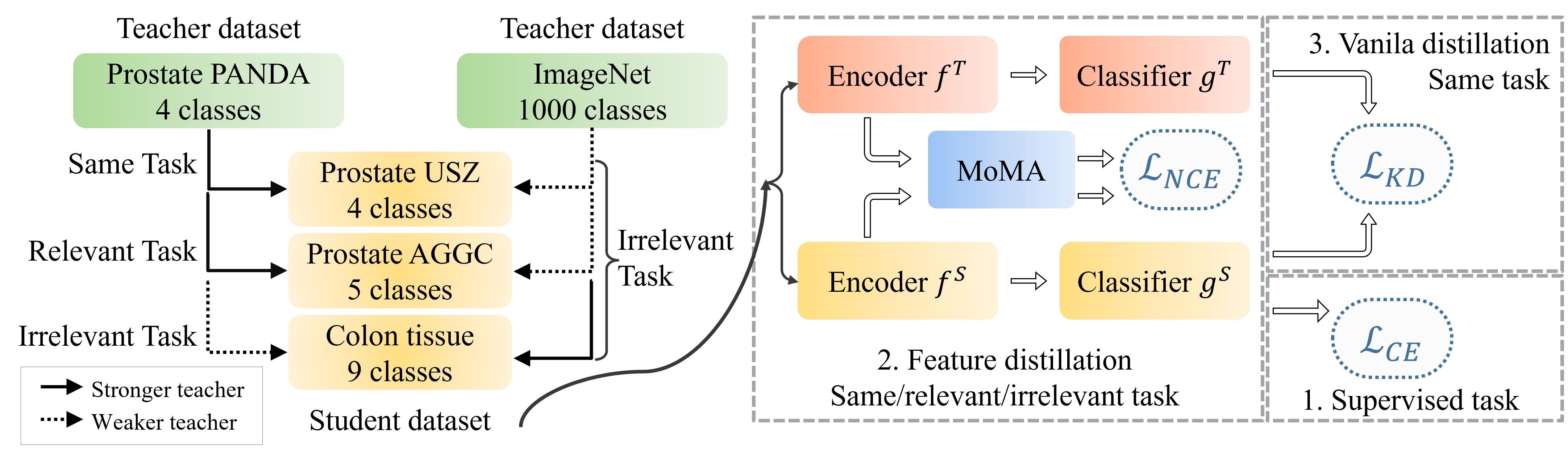
Figure 2: Overview of distillation flow across different tasks and datasets. 1) Supervised task is always conducted, 2) Feature distillation is applied if a well-trained teacher model is available, and 3) Vanilla ${L}_{KD}$ is employed if teacher and student models conduct the same task.

IV-C Experimental design

In order to evaluate the effectiveness of MoMA, we conduct three types of distillation tasks: 1) same task distillation: distillation between prostate cancer classification models, 2) relevant task distillation: distillation from 4-class prostate cancer classification to 5-class prostate cancer classification, and 3) irrelevant task distillation: distillation from prostate cancer classification to colon tissue type classification. Fig. 2 illustrates the distillation flow and the associated datasets and models.

We also compare MoMA with three different types of competing methods:

• Transfer Learning ($TL$): 1) TC_PANDA: $f^{T}$ trained on PANDA without fine-tuning on student datasets, 2) ST_no: $f^{S}$ without pre-trained weights, 3) ST_ImageNet: $f^{S}$ with pre-trained weights on ImageNet, 4) ST_PANDA: $f^{S}$ with pre-trained weights on PANDA.

• Logits distillation ($LD$): 1) Vanilla KD [18]: $f^{S}$ with vanilla KD method, 2) SimKD [89]: $f^{S}$ with re-used $g^{T}$ but no vanilla KD. Vanilla KD and SimKD are only applied to the same task distillation experiments due to the usage of $g^{T}$.

• Feature-Map/Embedding Distillation ($FD$): 1) FitNet [90], 2) AT [44], 3) SemCKD [45], 4) CC [48], and 5) CRD [19].

Moreover, we carry out an ablation study without utilizing MSA (MoMA w/o MSA) to investigate the influence of MSA on strengthening feature representations.

IV-D Quantitative evaluation

We evaluate MoMA and its competing models on the three distillation tasks using 1) Accuracy (ACC), 2) Macro-average F1 (F1), and 3) quadratic weighted kappa ($\kappa_{w}$). For the revelant distillation task on Prostate AGGC, we use weighted-average F1, F1_w = 0.25 * F1_G3 + 0.25 * F1_G4 +0.25 * F1_G5 +0.125 * F1_Normal +0.125 * F1_Stroma, which is the evaluation metric in the AGGC22 challenge.

V Experimental results

V-A Same task distillation: prostate cancer classification

TABLE I: Results of same task distillation. KL denotes the use of KL divergence loss.

			Prostate USZ (Test I)			Prostate UBC (Test II)
Method	Pretrained	ACC($\%$)	F1	$\kappa_{w}$	ACC($\%$)	F1	$\kappa_{w}$
TCPANDA	ImageNet	$63.4$	$0.526$	$0.531$	$78.2$	$0.580$	$0.680$
ST	None	$66.4\pm 1.600$	$0.566\pm 0.012$	$0.551\pm 0.020$	$31.7\pm 9.600$	$0.239\pm 0.073$	$0.143\pm 0.104$
ST	ImageNet	$67.0\pm 2.600$	$0.612\pm 0.027$	$0.604\pm 0.016$	$71.0\pm 2.800$	$0.592\pm 0.026$	$0.619\pm 0.036$
ST	PANDA	$72.7\pm 1.100$	$\textbf{0.687}\pm\textbf{0.009}$	$\textbf{0.671}\pm\textbf{0.005}$	$73.1\pm 1.900$	$0.599\pm 0.023$	$0.654\pm 0.031$
FitNet [43]	PANDA	$65.7\pm 3.600$	$0.574\pm 0.048$	$0.559\pm 0.056$	$34.5\pm 19.500$	$0.260\pm 0.150$	$0.139\pm 0.131$
AT [44]	PANDA	$71.2\pm 1.600$	$0.653\pm 0.021$	$0.652\pm 0.023$	$76.0\pm 3.500$	$0.628\pm 0.038$	$0.660\pm 0.053$
CC [48]	PANDA	$69.4\pm 1.400$	$0.624\pm 0.016$	$0.608\pm 0.026$	$51.9\pm 12.600$	$0.392\pm 0.100$	$0.268\pm 0.179$
CRD [19]	PANDA	$70.9\pm 0.700$	$0.642\pm 0.012$	$0.639\pm 0.015$	$70.7\pm 3.500$	$0.577\pm 0.032$	$0.610\pm 0.046$
SemCKD [45]	PANDA	$69.8\pm 1.000$	$0.638\pm 0.013$	$0.635\pm 0.007$	$75.4\pm 1.700$	$0.627\pm 0.009$	$0.685\pm 0.017$
MoMA (Ours)	ImageNet	$67.3\pm 3.400$	$0.617\pm 0.013$	$0.594\pm 0.028$	$65.4\pm 5.800$	$0.534\pm 0.059$	$0.533\pm 0.128$
MoMA (Ours)	PANDA	$\textbf{73.6}\pm\textbf{1.000}$	$0.687\pm 0.011$	$0.670\pm 0.010$	$75.5\pm 1.800$	$0.622\pm 0.019$	$0.666\pm 0.015$
Vanilla KD [18]	PANDA	$69.2\pm 0.400$	$0.596\pm 0.008$	$0.593\pm 0.005$	$82.9\pm 0.500$	$0.649\pm 0.013$	$0.74\pm 0.013$
SimKD [89]	PANDA	$65.9\pm 0.300$	$0.420\pm 0.001$	$0.413\pm 0.004$	$79.8\pm 0.100$	$0.586\pm 0.001$	$0.673\pm 0.002$
KL+FitNet [43]	PANDA	$68.7\pm 1.400$	$0.583\pm 0.030$	$0.585\pm 0.031$	$61.2\pm 27.000$	$0.452\pm 0.211$	$0.437\pm 0.279$
KL+AT [44]	PANDA	$68.7\pm 1.100$	$0.586\pm 0.017$	$0.593\pm 0.014$	$82.0\pm 1.100$	$0.650\pm 0.009$	$0.728\pm 0.018$
KL+CC [48]	PANDA	$68.6\pm 0.700$	$0.586\pm 0.016$	$0.589\pm 0.013$	$81.8\pm 0.900$	$0.630\pm 0.015$	$0.725\pm 0.017$
KL+CRD [19]	PANDA	$69.2\pm 1.000$	$0.595\pm 0.020$	$0.586\pm 0.010$	$82.3\pm 1.700$	$0.640\pm 0.016$	$0.728\pm 0.036$
KL+SemCKD [45]	PANDA	$68.9\pm 0.400$	$0.595\pm 0.004$	$0.596\pm 0.002$	$81.9\pm 0.800$	$\textbf{0.652}\pm\textbf{0.014}$	$0.734\pm 0.010$
KL+MoMA (Ours)	ImageNet	$70.3\pm 0.600$	$0.640\pm 0.019$	$0.618\pm 0.011$	$72.9\pm 3.500$	$0.585\pm 0.035$	$0.626\pm 0.027$
KL+MoMA (Ours)	PANDA	$72.2\pm 0.600$	$0.638\pm 0.018$	$0.618\pm 0.014$	$\textbf{83.3}\pm\textbf{0.800}$	$0.648\pm 0.016$	$\textbf{0.763}\pm\textbf{0.009}$

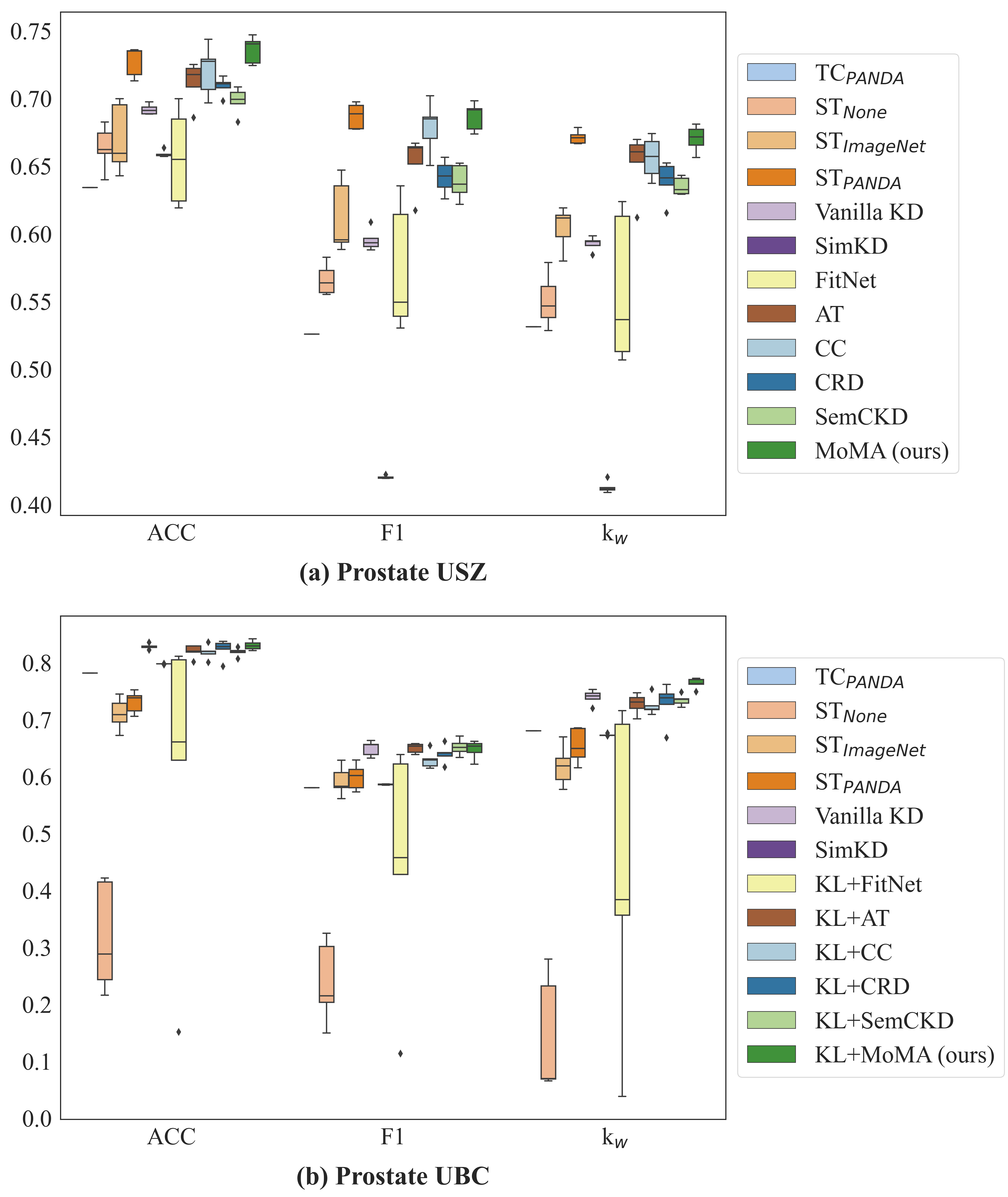
Figure 3: Bar plots for same task distillation: All the KD models utilize the pre-trained weights from PANDA.

Table I and Fig. 3 show the results of MoMA and its competitors on the two TMA prostate datasets (Prostate USZ and Prostate UBC). On Prostate USZ, the teacher model TC_PANDA, which was trained on PANDA only, achieved 63.4 $\%$ ACC, 0.526 F1, and 0.531 $\kappa_{w}$, which is substantially lower to other student models with $TL$, $LD$, and $FD$. Among the student models with $TL$, the student model with no pre-trained weights (ST_None) was inferior to other two student models; the student model pre-trained on PANDA (ST_PANDA) outperformed the student model pre-trained on ImageNet (ST_ImageNet). These indicate the importance of pre-trained weights and fine-tuning on the target dataset, i.e., Prostate USZ. As for the KD approaches, MoMA_PANDA, pre-trained on PANDA, outperformed all other KD methods, achieving ACC of 73.6 %, which is 0.9 % higher than ST_PANDA, and F1 of 0.687 and $\kappa_{w}$ of 0.670, which are comparable to those of ST_PANDA.

On the independent test set, Prostate UBC, it is remarkable that TC_PANDA achieved 78.2 $\%$ ACC and 0.680 $\kappa_{w}$, which are superior to those of all the student models with $TL$, likely suggesting that the characteristics of PANDA is more similar to Prostate UBC than Prostate USZ. The performance of the student models with $TL$ and $FD$ was similar to each other between Prostate USZ and Prostate UBC; for instance, MoMA_PANDA obtained higher ACC but lower F1 and $\kappa_{w}$ on Prostate UBC than on Prostate USZ. As MoMA and other student models with $FD$ adopt vanilla KD by setting $\gamma$ to 1 in $\mathcal{L}$, i.e., mimicking the output logits of the teacher model, there was, in general, a substantial increase in the performance on Prostate UBC. MoMA_PANDA, in particular, achieved the highest ACC of 83.3 % and $\kappa_{w}$ of 0.763 over all models under consideration, which are 11.1 % and 0.145 higher than those on Prostae USZ in ACC and $\kappa_{w}$, respectively.

V-B Relevant task distillation: prostate cancer classification

TABLE II: Results of relevant task distillation.

			AGGC CV (Test I)			AGGC test (Test II)
Method	Pretrained	ACC($\%$)	F1w	$\kappa_{w}$	ACC($\%$)	F1w	$\kappa_{w}$
ST	None	$74.0\pm 3.700$	$0.644\pm 0.039$	$0.774\pm 0.043$	$62.8\pm 1.000$	$0.483\pm 0.021$	$0.483\pm 0.089$
ST	ImageNet	$73.8\pm 4.500$	$0.645\pm 0.057$	$0.764\pm 0.043$	$76.0\pm 2.100$	$0.593\pm 0.012$	$0.770\pm 0.042$
ST	PANDA	$76.6\pm 2.800$	$0.660\pm 0.025$	$0.792\pm 0.031$	$76.5\pm 1.900$	$0.603\pm 0.013$	$0.771\pm 0.036$
FitNet [43]	PANDA	$74.2\pm 4.500$	$0.638\pm 0.050$	$0.774\pm 0.037$	$69.6\pm 7.600$	$0.554\pm 0.044$	$0.653\pm 0.095$
AT [44]	PANDA	$75.3\pm 3.000$	$0.649\pm 0.053$	$0.782\pm 0.046$	$74.3\pm 3.400$	$0.583\pm 0.017$	$0.779\pm 0.038$
CC [48]	PANDA	$\textbf{77.4}\pm\textbf{3.000}$	$0.668\pm 0.352$	$0.796\pm 0.350$	$77.2\pm 1.500$	$0.603\pm 0.016$	$0.760\pm 0.007$
CRD [19]	PANDA	$76.7\pm 2.700$	$0.663\pm 0.040$	$0.796\pm 0.036$	$\textbf{77.3}\pm\textbf{4.000}$	$0.602\pm 0.033$	$0.789\pm 0.029$
SemCKD [45]	PANDA	$74.1\pm 5.800$	$0.639\pm 0.043$	$0.762\pm 0.058$	$65.7\pm 13.300$	$0.532\pm 0.087$	$0.642\pm 0.107$
MoMA (Our)	ImageNet	$75.7\pm 4.800$	$0.663\pm 0.054$	$0.772\pm 0.035$	$75.5\pm 3.500$	$0.587\pm 0.019$	$0.788\pm 0.021$
MoMA (Our)	PANDA	$77.1\pm 2.000$	$\textbf{0.670}\pm\textbf{0.042}$	$\textbf{0.798}\pm\textbf{0.029}$	$77.1\pm 2.300$	$\textbf{0.609}\pm\textbf{0.015}$	$\textbf{0.794}\pm\textbf{0.018}$

Figure 4: Bar plots for relevant task distillation. All the KD models utilize the pre-trained weights from PANDA.

Table II and Fig. 4 show the results of MoMA and its competing methods on relevant task distillation, i.e., distillation from 4-class prostate cancer classification to 5-class prostate cancer classification (Prostate AGGC22). The two tasks share 4 classes in common, and thus the direct application of the teacher model and logits distillation is infeasible. In the cross-validation experiments (AGGC CV), MoMA_PANDA, on average, achieved the best F1_w of 0.670 and $\kappa_{w}$ of 0.798 and obtained the second best ACC of 77.1 %. The performance of ST_PANDA was generally comparable to the student models with $FD$. Other student models with $TL$ were, by and large, inferior to the ones with $FD$. In a head-to-head comparison between Prostate AGGC CV and Prostate AGGC test, there was, in general, a slight performance drop, likely due to the differences in the type of images and scanners. Though there was a performance drop, similar trends were found across different models between AGGC CV and AGGC test. We also note that MoMA_PNADA, on average, was superior to all the competitors on two evaluation metrics (F1_w and $\kappa_{w}$) and attained the third best ACC, which is 0.2 % lower than CRD.

V-C Irrelevant task distillation: colon tissue type classification

TABLE III: Results of irrelevant task distillation.

			Colon K16 SN (Test I)			Colon K16 (Test II)
Method	Pretrained	ACC ($\%$)	F1	$\kappa_{w}$	ACC ($\%$)	F1	$\kappa_{w}$
ST	None	$76.8\pm 4.700$	$0.752\pm 0.057$	$0.871\pm 0.021$	$81.6\pm 1.900$	$0.814\pm 0.020$	$0.858\pm 0.011$
ST	ImageNet	$83.8\pm 0.600$	$0.834\pm 0.007$	$0.879\pm 0.007$	$86.2\pm 0.700$	$0.861\pm 0.008$	$0.898\pm 0.011$
ST	PANDA	$82.9\pm 0.700$	$0.827\pm 0.007$	$0.870\pm 0.006$	$83.2\pm 2.500$	$0.834\pm 0.023$	$0.848\pm 0.032$
FitNet [43]	ImageNet	$83.1\pm 0.700$	$0.826\pm 0.009$	$0.886\pm 0.005$	$83.2\pm 4.100$	$0.836\pm 0.038$	$0.853\pm 0.035$
AT [44]	ImageNet	$83.6\pm 0.700$	$0.832\pm 0.009$	$\textbf{0.889}\pm\textbf{0.002}$	$86.0\pm 1.600$	$0.861\pm 0.014$	$0.882\pm 0.028$
CC [48]	ImageNet	$83.9\pm 1.400$	$0.839\pm 0.014$	$0.859\pm 0.010$	$86.3\pm 0.900$	$0.862\pm 0.010$	$\textbf{0.898}\pm\textbf{0.008}$
CRD [19]	ImageNet	$81.6\pm 3.000$	$0.808\pm 0.038$	$0.885\pm 0.008$	$84.9\pm 2.700$	$0.846\pm 0.030$	$0.890\pm 0.017$
SemCKD [45]	ImageNet	$83.8\pm 0.800$	$0.837\pm 0.008$	$0.879\pm 0.007$	$80.8\pm 5.500$	$0.808\pm 0.058$	$0.847\pm 0.046$
MoMA (Ours)	ImageNet	$\textbf{85.2}\pm\textbf{0.600}$	$\textbf{0.850}\pm\textbf{0.006}$	$0.888\pm 0.006$	$\textbf{87.2}\pm\textbf{0.700}$	$\textbf{0.872}\pm\textbf{0.008}$	$0.898\pm 0.012$
MoMA (Ours)	PANDA	$82.5\pm 0.500$	$0.822\pm 0.004$	$0.867\pm 0.006$	$84.2\pm 0.900$	$0.844\pm 0.008$	$0.861\pm 0.020$

Figure 5: Bar plots for irrelevant task distillation. All the KD models utilize the pre-trained weights from ImageNet.

Table III and Fig. 5 show the results of distillation from 4-class prostate cancer classification to colon tissue type classification. Similar to the previous tasks, the student models either pre-trained on ImageNet ST_ImageNet or PANDA ST_PANDA were able to improve upon the model performance without pre-training. MoMA_ImageNet, utilizing the pre-trained weights of ImageNet, outperformed all the competing models except AT and CC in $\kappa_{w}$ for Colon K16 SN and Colon K16, respectively. It is worth noting that, for both $TL$ and $FD$ approaches, the effect of the pre-trained weights of ImageNet was larger than that of PANDA. ST_ImageNet was superior to ST_PANDA. Similarly, MoMA_ImageNet obtained better performance than MoMA_PANDA.

V-D Inter- and intra-class correlations for student and teacher models

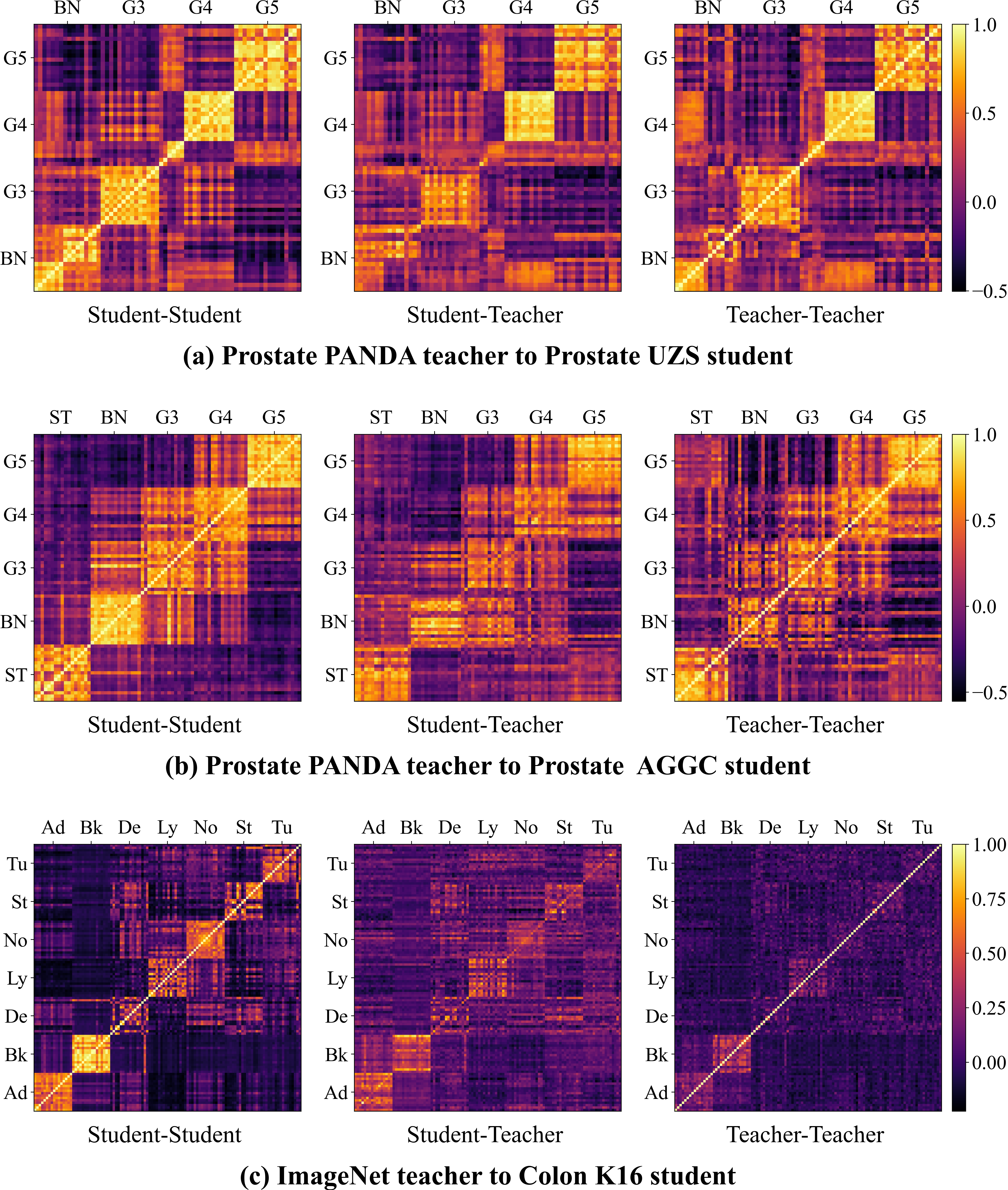
Figure 6: The correlation coefficient matrix between feature presentations of a teacher network and student network

Fig. 6 shows the inter- and intra-class correlations between feature embeddings encoded by the MoMA student and teacher models. Three types of correlations were measured, including student-to-student, student-to-teacher, and teacher-to-teacher correlations. As for the teacher model, we chose the best teacher model per task, i.e., the teacher models pre-trained on PANDA for two prostate cancer classification tasks and the ImageNet teacher model for the colon tissue type classification task. For each task, 16 samples per class were randomly chosen from the validation set.

For the three distillation tasks, the student models, in general, showed higher intra-class correlations and lower inter-class correlations, which explains the superior performance of the student models in the classification tasks. For instance, in the same task distillation, i.e., from PANDA to Prostate USZ, the PANDA teacher model was partially successful in demonstrating the connections between four different types of class labels; it had difficulties in distinguishing some samples in BN and G3, which can be shown by the lower intra-class correlations within B3 and G3. This is likely due to variations between the source and target datasets. However, the student model, trained on a target/student dataset, was able to achieve stronger intra-class correlations for both BN and G3 while still maintaining high intra-class correlations for G4 and G5; inter-class correlations were lowered in general. Similar observations were made for other two tasks. Such improvement, achieved through the MoMA framework, is not only due to the knowledge from the teacher model but also due to the utilization of the target dataset.

V-E Ablation study

TABLE IV: Ablation results compare the performance of MoMA with and without Multi-head Attention on the three tasks.

			Test I			Test II
Task	Method	ACC	F1	$\kappa_{w}$	ACC	F1	$\kappa_{w}$
Same task	MoMA w/o MSA	$72.0\pm 0.400$	$0.663\pm 0.004$	$0.654\pm 0.008$	$73.8\pm 1.700$	$0.616\pm 0.014$	$\textbf{0.667}\pm\textbf{0.012}$
distillation	MoMA	$\textbf{73.6}\pm\textbf{1.000}$	$\textbf{ 0.687}\pm\textbf{0.011}$	$\textbf{0.670}\pm\textbf{0.010 }$	$\textbf{75.5}\pm\textbf{1.800}$	$\textbf{0.622}\pm\textbf{0.019 }$	$0.666\pm 0.015$
Relevant task	MoMA w/o MSA	$75.6\pm 1.200$	$0.649\pm 0.036$	$0.786\pm 0.045$	$\textbf{77.2}\pm\textbf{2.400}$	$0.601\pm 0.02$	$\textbf{ 0.804}\pm\textbf{0.042}$
distillation	MoMA	$\textbf{77.1}\pm\textbf{ 2.000}$	$\textbf{0.670}\pm\textbf{0.042}$	$\textbf{0.798}\pm\textbf{0.029}$	$77.1\pm 2.300$	$\textbf{0.609}\pm\textbf{0.015}$	$0.794\pm 0.018$
Irrelevant task	MoMA w/o MSA	$84.0\pm 0.400$	$0.838\pm 0.004$	$0.880\pm 0.005$	$85.5\pm 1.400$	$0.856\pm 0.015$	$\textbf{0.900}\pm\textbf{0.008}$
distillation	MoMA	$\textbf{85.2}\pm\textbf{0.600}$	$\textbf{0.850}\pm\textbf{0.006}$	$\textbf{0.888}\pm\textbf{0.006}$	$\textbf{87.2}\pm\textbf{0.700}$	$\textbf{ 0.872}\pm\textbf{0.008}$	$0.898\pm 0.012$

Table IV compares the performance of MoMA with and without MSA across three distillation tasks. The results demonstrate the crucial role of MSA in the proposed approach. MoMA without MSA, in general, experienced a performance drop for the three distillation tasks. Without MSA, MoMA was able to achieve the better or comparable performance to other competing models across different distillation tasks, suggesting the effectiveness and robustness of the proposed framework.

VI Discussion

In this work, we introduce an approach of KD, so called MoMA, to build an optimal model for a target histopathology dataset using the existing models on similar, relevant, and irrelevant tasks. The experiment results show that MoMA offers advancements in distilling knowledge for the three classification tasks. Regardless of the type of the distillation tasks, MoMA enables the student model to inherit feature extraction capabilities from the teacher model and to conduct accurate classification for the target task. Exploiting the knowledge from both the source and target datasets, MoMA also provides the superior generalizability on unseen, independent test sets across three different tasks.

The aim of this work is to propose a method to distill the knowledge from the source/teacher domain to the target domain without direct access to the source data. Transferring only the teacher model is more feasible in various contexts; for instance, when the source data is enormous in size, like ImageNet, it is time-consuming and inefficient to train a model using such source data; healthcare data, including pathology images, is restricted for security and privacy reasons, and thus transferring to target data centers or hospitals is likely to be infeasible. In such circumstances, KD is a key to resolve all the related issues. In the distillation, we emphasize that the choice of the pre-trained teacher model is crucial as it directly impacts the performance of the target model. Based on the experimental results across different classification tasks, it is evident that the better the teacher model is, the greater benefits to the student model it provides.

The proposed MoMA framework is an end-to-end training approach, eliminating the need for extensive training of the self-supervised task followed by fine-tuning on labeled datasets. Moreover, self-supervised methods require a large amount of training data which is not always available in medical/pathology image analysis. Leveraging the high-quality teacher model through MoMA facilitates robust training and convergence of the student model on smaller target datasets. Furthermore, the excellence performance in the relevant and irrelevant tasks suggests that MoMA could be utilized solely as a feature-embedding distillation mechanism without requiring a meticulous redesign of the model architecture and distillation framework in response to the specific requirement of downstream tasks.

In the ablation study, the role of MSA was apparent in MoMA. The previous SSCL assumed that all samples are equally important. However, depending on the appearance and characteristics of an image and the extent of augmentation applied, the classification task may become easier or more challenging. By incorporating MSA, MoMA gains the ability to selectively focus on important samples while allocating less attention to other samples. It is worth noting that the contrastive loss $\mathcal{L}_{NCE}$ does not treat each input sample independently, unlike the supervised cross-entropy loss $\mathcal{L}_{CE}$. With MSA, MoMA learns the relationships among samples within a batch before they are fed into the self-supervised contrastive loss, and, in turn, used to update the queue $Z^{queue}$, prioritizing and enriching the information within these samples and allowing for more effective optimization of the model.

The results of the three distillation tasks, i.e., the same task, relevant task, and irrelevant task, provide insights into the distillation of knowledge from the source domain to the target domain and the model development for the target domain. First, supervised learning on the target domain provides comparable performance in all three distillation tasks, but its performance on unseen data, i.e., generalizability, is not guaranteed. Second, the usage of the pre-trained weights is crucial for both TL and KD, regardless of the type of distillation tasks. Third, the effect of the pre-trained weights depends on the type of distillation tasks. As for the same and relevant tasks, the pre-trained weights from the same or relevant tasks were more useful. For the irrelevant task, the pre-trained weights from ImageNet were more beneficial than those from PANDA. These indicate that not all pathology image datasets will be helpful to build a model for a specific computational pathology task and a dataset. Last, the KD strategy varies across different distillation tasks. The same task distillation takes advantage of the logits distillation, the relevant task distillation exploits the pre-trained weights, and the irrelevant task distillation does not make use of the (irrelevant) domain-specific knowledge much.

There are several limitations in our work. First, we utilize ImageNet and PANDA as the source datasets. ImageNet is one of the most widely studied and utilized large-scale datasets. PANDA is one of the large-scale pathology image datasets, but it is limited to four classes in one organ. The larger and more diverse the pathology image dataset is, the better the distillation quality we could obtain. Second, three pathology image classification tasks from two organs were considered in this study. The effect of KD may vary depending on the type of tasks and organs. Third, there exist other types of image classification tasks in computational pathology such as survival/outcome prediction. In general, the amount of survival/outcome dataset is smaller than that of cancer and tissue classifications, and thus KD may play a crucial role in survival/outcome prediction. Last, we only consider CNNs for the three distillation tasks. Several recent studies have shown that transformer-based models such as Vision Transformer (ViT) outperformed CNN-based models on image classification tasks. Evaluating the proposed MoMA on different teacher-student combinations like ViT teacher to ViT student and CNN teacher to ViT student could provide valuable insights into the effectiveness of the proposed method across different architectures. In order to focus on KD, we conduct our study on CNNs and leave the study involving transformer-based models for future research.

VII Conclusions

Herein, we propose an efficient and effective learning framework called MoMA to build an accurate and robust classification model in pathology images. Exploiting the KD framework, momentum contrastive learning, and SA, MoMA was able to transfer knowledge from a source domain to a target domain and to learn a robust classification model for three different tasks. Moreover, the experimental results of MoMA suggest an adequate learning strategy for different distillation tasks and scenarios. We anticipate that this will be a great help in developing computational pathology tools for various tasks. Future studies will entail the further investigation of the efficient KD method and extended validation and application of MoMA to other types of datasets and tasks in computational pathology.

References

- [1] M. Cui and D. Y. Zhang, “Artificial intelligence and computational pathology,” Laboratory Investigation, vol. 101, no. 4, pp. 412–422, 2021.
- [2] S. Graham, Q. D. Vu, S. E. A. Raza, A. Azam, Y. W. Tsang, J. T. Kwak, and N. Rajpoot, “Hover-net: Simultaneous segmentation and classification of nuclei in multi-tissue histology images,” Medical Image Analysis, vol. 58, p. 101563, 2019.
- [3] N. Marini, S. Otálora, H. Müller, and M. Atzori, “Semi-supervised training of deep convolutional neural networks with heterogeneous data and few local annotations: An experiment on prostate histopathology image classification,” Medical image analysis, vol. 73, p. 102165, 2021.
- [4] P. Chunduru, J. J. Phillips, and A. M. Molinaro, “Prognostic risk stratification of gliomas using deep learning in digital pathology images,” Neuro-oncology advances, vol. 4, no. 1, p. vdac111, 2022.
- [5] Z. Huang, H. Chai, R. Wang, H. Wang, Y. Yang, and H. Wu, “Integration of patch features through self-supervised learning and transformer for survival analysis on whole slide images,” in Medical Image Computing and Computer Assisted Intervention–MICCAI 2021: 24th International Conference, Strasbourg, France, September 27–October 1, 2021, Proceedings, Part VIII 24. Springer, 2021, pp. 561–570.
- [6] L. Li, Y. Liang, M. Shao, S. Lu, D. Ouyang et al., “Self-supervised learning-based multi-scale feature fusion network for survival analysis from whole slide images,” Computers in Biology and Medicine, vol. 153, p. 106482, 2023.
- [7] K. Stacke, G. Eilertsen, J. Unger, and C. Lundström, “Measuring domain shift for deep learning in histopathology,” IEEE journal of biomedical and health informatics, vol. 25, no. 2, pp. 325–336, 2020.
- [8] M. Aubreville, N. Stathonikos, C. A. Bertram, R. Klopfleisch, N. Ter Hoeve, F. Ciompi, F. Wilm, C. Marzahl, T. A. Donovan, A. Maier et al., “Mitosis domain generalization in histopathology images—the midog challenge,” Medical Image Analysis, vol. 84, p. 102699, 2023.
- [9] B. Ghorbani, O. Firat, M. Freitag, A. Bapna, M. Krikun, X. Garcia, C. Chelba, and C. Cherry, “Scaling laws for neural machine translation,” in International Conference on Learning Representations, 2022. [Online]. Available: https://openreview.net/forum?id=hR_SMu8cxCV
- [10] X. Zhai, A. Kolesnikov, N. Houlsby, and L. Beyer, “Scaling vision transformers,” in Proceedings of the IEEE/CVF Conference on Computer Vision and Pattern Recognition, 2022, pp. 12 104–12 113.
- [11] M. Dehghani, J. Djolonga, B. Mustafa, P. Padlewski, J. Heek, J. Gilmer, A. Steiner, M. Caron, R. Geirhos, I. Alabdulmohsin et al., “Scaling vision transformers to 22 billion parameters,” arXiv preprint arXiv:2302.05442, 2023.
- [12] J. N. Kather, J. Krisam, P. Charoentong, T. Luedde, E. Herpel, C.-A. Weis, T. Gaiser, A. Marx, N. A. Valous, D. Ferber et al., “Predicting survival from colorectal cancer histology slides using deep learning: A retrospective multicenter study,” PLoS medicine, vol. 16, no. 1, p. e1002730, 2019.
- [13] T. N. Doan, B. Song, T. T. Vuong, K. Kim, and J. T. Kwak, “Sonnet: A self-guided ordinal regression neural network for segmentation and classification of nuclei in large-scale multi-tissue histology images,” IEEE Journal of Biomedical and Health Informatics, vol. 26, no. 7, pp. 3218–3228, 2022.
- [14] W. Bulten, K. Kartasalo, P.-H. C. Chen, P. Ström, H. Pinckaers, K. Nagpal, Y. Cai, D. F. Steiner, H. van Boven, R. Vink et al., “Artificial intelligence for diagnosis and gleason grading of prostate cancer: the panda challenge,” Nature medicine, vol. 28, no. 1, pp. 154–163, 2022.
- [15] M. R. Hosseinzadeh Taher, F. Haghighi, R. Feng, M. B. Gotway, and J. Liang, “A systematic benchmarking analysis of transfer learning for medical image analysis,” in Domain Adaptation and Representation Transfer, and Affordable Healthcare and AI for Resource Diverse Global Health: Third MICCAI Workshop, DART 2021, and First MICCAI Workshop, FAIR 2021, Held in Conjunction with MICCAI 2021, Strasbourg, France, September 27 and October 1, 2021, Proceedings 3. Springer, 2021, pp. 3–13.
- [16] A. Dosovitskiy, L. Beyer, A. Kolesnikov, D. Weissenborn, X. Zhai, T. Unterthiner, M. Dehghani, M. Minderer, G. Heigold, S. Gelly, J. Uszkoreit, and N. Houlsby, “An image is worth 16x16 words: Transformers for image recognition at scale,” in International Conference on Learning Representations, 2021. [Online]. Available: https://openreview.net/forum?id=YicbFdNTTy
- [17] X. Li and K. N. Plataniotis, “How much off-the-shelf knowledge is transferable from natural images to pathology images?” Plos one, vol. 15, no. 10, p. e0240530, 2020.
- [18] G. Hinton, O. Vinyals, and J. Dean, “Distilling the knowledge in a neural network,” arXiv preprint arXiv:1503.02531, 2015.
- [19] Y. Tian, D. Krishnan, and P. Isola, “Contrastive representation distillation,” in International Conference on Learning Representations, 2020. [Online]. Available: https://openreview.net/forum?id=SkgpBJrtvS
- [20] Z. Yuan, X. Yan, Y. Liao, Y. Guo, G. Li, S. Cui, and Z. Li, “X-trans2cap: Cross-modal knowledge transfer using transformer for 3d dense captioning,” in Proceedings of the IEEE/CVF Conference on Computer Vision and Pattern Recognition, 2022, pp. 8563–8573.
- [21] S. M. Ahmed, S. Lohit, K.-C. Peng, M. J. Jones, and A. K. Roy-Chowdhury, “Cross-modal knowledge transfer without task-relevant source data,” in Computer Vision–ECCV 2022: 17th European Conference, Tel Aviv, Israel, October 23–27, 2022, Proceedings, Part XXXIV. Springer, 2022, pp. 111–127.
- [22] L. Zhao, X. Peng, Y. Chen, M. Kapadia, and D. N. Metaxas, “Knowledge as priors: Cross-modal knowledge generalization for datasets without superior knowledge,” in Proceedings of the IEEE/CVF Conference on Computer Vision and Pattern Recognition, 2020, pp. 6528–6537.
- [23] S. Du, S. You, X. Li, J. Wu, F. Wang, C. Qian, and C. Zhang, “Agree to disagree: Adaptive ensemble knowledge distillation in gradient space,” advances in neural information processing systems, vol. 33, pp. 12 345–12 355, 2020.
- [24] T. Lin, L. Kong, S. U. Stich, and M. Jaggi, “Ensemble distillation for robust model fusion in federated learning,” Advances in Neural Information Processing Systems, vol. 33, pp. 2351–2363, 2020.
- [25] Z. Allen-Zhu and Y. Li, “Towards understanding ensemble, knowledge distillation and self-distillation in deep learning,” in The Eleventh International Conference on Learning Representations, 2023. [Online]. Available: https://openreview.net/forum?id=Uuf2q9TfXGA
- [26] L. Gorelick, O. Veksler, M. Gaed, J. A. Gómez, M. Moussa, G. Bauman, A. Fenster, and A. D. Ward, “Prostate histopathology: Learning tissue component histograms for cancer detection and classification,” IEEE transactions on medical imaging, vol. 32, no. 10, pp. 1804–1818, 2013.
- [27] S. Doyle, M. D. Feldman, N. Shih, J. Tomaszewski, and A. Madabhushi, “Cascaded discrimination of normal, abnormal, and confounder classes in histopathology: Gleason grading of prostate cancer,” BMC bioinformatics, vol. 13, pp. 1–15, 2012.
- [28] J. N. Kather, C.-A. Weis, F. Bianconi, S. M. Melchers, L. R. Schad, T. Gaiser, A. Marx, and F. G. Zöllner, “Multi-class texture analysis in colorectal cancer histology,” Scientific reports, vol. 6, no. 1, pp. 1–11, 2016.
- [29] R. Sarkar and S. T. Acton, “Sdl: Saliency-based dictionary learning framework for image similarity,” IEEE Transactions on Image Processing, vol. 27, no. 2, pp. 749–763, 2017.
- [30] A. Paul, A. Dey, D. P. Mukherjee, J. Sivaswamy, and V. Tourani, “Regenerative random forest with automatic feature selection to detect mitosis in histopathological breast cancer images,” in Medical Image Computing and Computer-Assisted Intervention–MICCAI 2015: 18th International Conference, Munich, Germany, October 5-9, 2015, Proceedings, Part II 18. Springer, 2015, pp. 94–102.
- [31] M. A. Kahya, W. Al-Hayani, and Z. Y. Algamal, “Classification of breast cancer histopathology images based on adaptive sparse support vector machine,” Journal of Applied Mathematics and Bioinformatics, vol. 7, no. 1, p. 49, 2017.
- [32] A. Nguyen, D. Moore, I. McCowan, and M.-J. Courage, “Multi-class classification of cancer stages from free-text histology reports using support vector machines,” in 2007 29th Annual International Conference of the IEEE Engineering in Medicine and Biology Society. IEEE, 2007, pp. 5140–5143.
- [33] J. T. Kwak, S. M. Hewitt, S. Sinha, and R. Bhargava, “Multimodal microscopy for automated histologic analysis of prostate cancer,” BMC cancer, vol. 11, no. 1, pp. 1–16, 2011.
- [34] C. Li, X. Wang, W. Liu, and L. J. Latecki, “Deepmitosis: Mitosis detection via deep detection, verification and segmentation networks,” Medical image analysis, vol. 45, pp. 121–133, 2018.
- [35] T. T. Le Vuong, B. Song, J. T. Kwak, and K. Kim, “Prediction of epstein-barr virus status in gastric cancer biopsy specimens using a deep learning algorithm,” JAMA Network Open, vol. 5, no. 10, pp. e2 236 408–e2 236 408, 2022.
- [36] S. Graham, Q. D. Vu, M. Jahanifar, S. E. A. Raza, F. Minhas, D. Snead, and N. Rajpoot, “One model is all you need: multi-task learning enables simultaneous histology image segmentation and classification,” Medical Image Analysis, vol. 83, p. 102685, 2023.
- [37] T. T. Vuong, B. Song, K. Kim, Y. M. Cho, and J. T. Kwak, “Multi-scale binary pattern encoding network for cancer classification in pathology images,” IEEE Journal of Biomedical and Health Informatics, vol. 26, no. 3, pp. 1152–1163, 2021.
- [38] H. Wu, Z. Wang, Y. Song, L. Yang, and J. Qin, “Cross-patch dense contrastive learning for semi-supervised segmentation of cellular nuclei in histopathologic images,” in Proceedings of the IEEE/CVF Conference on Computer Vision and Pattern Recognition, 2022, pp. 11 666–11 675.
- [39] X. Shi, H. Su, F. Xing, Y. Liang, G. Qu, and L. Yang, “Graph temporal ensembling based semi-supervised convolutional neural network with noisy labels for histopathology image analysis,” Medical image analysis, vol. 60, p. 101624, 2020.
- [40] T. J. Fuchs and J. M. Buhmann, “Computational pathology: challenges and promises for tissue analysis,” Computerized Medical Imaging and Graphics, vol. 35, no. 7-8, pp. 515–530, 2011.
- [41] S. Shinde, U. Kulkarni, D. Mane, and A. Sapkal, “Deep learning-based medical image analysis using transfer learning,” Health Informatics: A Computational Perspective in Healthcare, pp. 19–42, 2021.
- [42] M. A. Morid, A. Borjali, and G. Del Fiol, “A scoping review of transfer learning research on medical image analysis using imagenet,” Computers in biology and medicine, vol. 128, p. 104115, 2021.
- [43] A. Romero, N. Ballas, S. E. Kahou, A. Chassang, C. Gatta, and Y. Bengio, “Fitnets: Hints for thin deep nets,” in 3rd International Conference on Learning Representations, ICLR 2015, San Diego, CA, USA, May 7-9, 2015, Conference Track Proceedings, Y. Bengio and Y. LeCun, Eds., 2015. [Online]. Available: http://arxiv.org/abs/1412.6550
- [44] N. Komodakis, S. Zagoruyko, and , “Paying more attention to attention: improving the performance of convolutional neural networks via attention transfer,” in ICLR, 2017.
- [45] C. Wang, D. Chen, J.-P. Mei, Y. Zhang, Y. Feng, and C. Chen, “Semckd: semantic calibration for cross-layer knowledge distillation,” IEEE Transactions on Knowledge and Data Engineering, 2022.
- [46] Z. Huang and N. Wang, “Like what you like: Knowledge distill via neuron selectivity transfer,” arXiv preprint arXiv:1707.01219, 2017.
- [47] N. Passalis, M. Tzelepi, and A. Tefas, “Probabilistic knowledge transfer for lightweight deep representation learning,” IEEE Transactions on Neural Networks and Learning Systems, vol. 32, no. 5, pp. 2030–2039, 2020.
- [48] B. Peng, X. Jin, J. Liu, D. Li, Y. Wu, Y. Liu, S. Zhou, and Z. Zhang, “Correlation congruence for knowledge distillation,” in Proceedings of the IEEE/CVF International Conference on Computer Vision, 2019, pp. 5007–5016.
- [49] G. Xu, Z. Liu, X. Li, and C. C. Loy, “Knowledge distillation meets self-supervision,” in Computer Vision–ECCV 2020: 16th European Conference, Glasgow, UK, August 23–28, 2020, Proceedings, Part IX. Springer, 2020, pp. 588–604.
- [50] F. M. Thoker and J. Gall, “Cross-modal knowledge distillation for action recognition,” in 2019 IEEE International Conference on Image Processing (ICIP). IEEE, 2019, pp. 6–10.
- [51] A. Malinin, B. Mlodozeniec, and M. Gales, “Ensemble distribution distillation,” arXiv preprint arXiv:1905.00076, 2019.
- [52] H. Touvron, M. Cord, M. Douze, F. Massa, A. Sablayrolles, and H. Jégou, “Training data-efficient image transformers & distillation through attention,” in International conference on machine learning. PMLR, 2021, pp. 10 347–10 357.
- [53] I. Radosavovic, R. P. Kosaraju, R. Girshick, K. He, and P. Dollár, “Designing network design spaces,” in Proceedings of the IEEE/CVF conference on computer vision and pattern recognition, 2020, pp. 10 428–10 436.
- [54] A. Dosovitskiy, L. Beyer, A. Kolesnikov, D. Weissenborn, X. Zhai, T. Unterthiner, M. Dehghani, M. Minderer, G. Heigold, S. Gelly et al., “An image is worth 16x16 words: Transformers for image recognition at scale,” arXiv preprint arXiv:2010.11929, 2020.
- [55] J. M. Noothout, N. Lessmann, M. C. Van Eede, L. D. van Harten, E. Sogancioglu, F. G. Heslinga, M. Veta, B. van Ginneken, and I. Išgum, “Knowledge distillation with ensembles of convolutional neural networks for medical image segmentation,” Journal of Medical Imaging, vol. 9, no. 5, pp. 052 407–052 407, 2022.
- [56] S. Javed, A. Mahmood, T. Qaiser, and N. Werghi, “Knowledge distillation in histology landscape by multi-layer features supervision,” IEEE Journal of Biomedical and Health Informatics, 2023.
- [57] S. Shaw, M. Pajak, A. Lisowska, S. A. Tsaftaris, and A. Q. O’Neil, “Teacher-student chain for efficient semi-supervised histology image classification,” arXiv preprint arXiv:2003.08797, 2020.
- [58] T. Hassan, M. Shafay, B. Hassan, M. U. Akram, A. ElBaz, and N. Werghi, “Knowledge distillation driven instance segmentation for grading prostate cancer,” Computers in Biology and Medicine, vol. 150, p. 106124, 2022.
- [59] J. DiPalma, A. A. Suriawinata, L. J. Tafe, L. Torresani, and S. Hassanpour, “Resolution-based distillation for efficient histology image classification,” Artificial Intelligence in Medicine, vol. 119, p. 102136, 2021.
- [60] S. Gidaris, P. Singh, and N. Komodakis, “Unsupervised representation learning by predicting image rotations,” arXiv preprint arXiv:1803.07728, 2018.
- [61] P. Goyal, D. Mahajan, A. Gupta, and I. Misra, “Scaling and benchmarking self-supervised visual representation learning,” in Proceedings of the ieee/cvf International Conference on computer vision, 2019, pp. 6391–6400.
- [62] M. Noroozi and P. Favaro, “Unsupervised learning of visual representations by solving jigsaw puzzles,” in European conference on computer vision. Springer, 2016, pp. 69–84.
- [63] T. Chen, S. Kornblith, M. Norouzi, and G. Hinton, “A simple framework for contrastive learning of visual representations,” in International conference on machine learning. PMLR, 2020, pp. 1597–1607.
- [64] Z. Wu, Y. Xiong, S. X. Yu, and D. Lin, “Unsupervised feature learning via non-parametric instance discrimination,” in Proceedings of the IEEE conference on computer vision and pattern recognition, 2018, pp. 3733–3742.
- [65] K. He, H. Fan, Y. Wu, S. Xie, and R. Girshick, “Momentum contrast for unsupervised visual representation learning,” in Proceedings of the IEEE/CVF conference on computer vision and pattern recognition, 2020, pp. 9729–9738.
- [66] C. Chen, J. Zhang, Y. Xu, L. Chen, J. Duan, Y. Chen, S. D. Tran, B. Zeng, and T. Chilimbi, “Why do we need large batchsizes in contrastive learning? a gradient-bias perspective,” in Advances in Neural Information Processing Systems, A. H. Oh, A. Agarwal, D. Belgrave, and K. Cho, Eds., 2022. [Online]. Available: https://openreview.net/forum?id=T1dhAPdS--
- [67] O. Ciga, T. Xu, and A. L. Martel, “Self supervised contrastive learning for digital histopathology,” Machine Learning with Applications, vol. 7, p. 100198, 2022.
- [68] T. T. L. Vuong, Q. D. Vu, M. Jahanifar, S. Graham, J. T. Kwak, and N. Rajpoot, “Impash: A novel domain-shift resistant representation for colorectal cancer tissue classification,” in Computer Vision–ECCV 2022 Workshops: Tel Aviv, Israel, October 23–27, 2022, Proceedings, Part III. Springer, 2023, pp. 543–555.
- [69] J. Li, Y. Zheng, K. Wu, J. Shi, F. Xie, and Z. Jiang, “Lesion-aware contrastive representation learning for histopathology whole slide images analysis,” in Medical Image Computing and Computer Assisted Intervention–MICCAI 2022: 25th International Conference, Singapore, September 18–22, 2022, Proceedings, Part II. Springer, 2022, pp. 273–282.
- [70] P. Yang, X. Yin, H. Lu, Z. Hu, X. Zhang, R. Jiang, and H. Lv, “Cs-co: A hybrid self-supervised visual representation learning method for h&e-stained histopathological images,” Medical Image Analysis, vol. 81, p. 102539, 2022.
- [71] M. Jaderberg, K. Simonyan, A. Zisserman et al., “Spatial transformer networks,” Advances in neural information processing systems, vol. 28, 2015.
- [72] J. Hu, L. Shen, and G. Sun, “Squeeze-and-excitation networks,” in Proceedings of the IEEE conference on computer vision and pattern recognition, 2018, pp. 7132–7141.
- [73] Z. Huang, X. Wang, L. Huang, C. Huang, Y. Wei, and W. Liu, “Ccnet: Criss-cross attention for semantic segmentation,” in Proceedings of the IEEE/CVF international conference on computer vision, 2019, pp. 603–612.
- [74] M. Bilal, R. Jewsbury, R. Wang, H. M. AlGhamdi, A. Asif, M. Eastwood, and N. Rajpoot, “An aggregation of aggregation methods in computational pathology,” Medical Image Analysis, p. 102885, 2023.
- [75] Y. Sharma, A. Shrivastava, L. Ehsan, C. A. Moskaluk, S. Syed, and D. Brown, “Cluster-to-conquer: A framework for end-to-end multi-instance learning for whole slide image classification,” in Medical Imaging with Deep Learning. PMLR, 2021, pp. 682–698.
- [76] N. Hashimoto, D. Fukushima, R. Koga, Y. Takagi, K. Ko, K. Kohno, M. Nakaguro, S. Nakamura, H. Hontani, and I. Takeuchi, “Multi-scale domain-adversarial multiple-instance cnn for cancer subtype classification with unannotated histopathological images,” in Proceedings of the IEEE/CVF conference on computer vision and pattern recognition, 2020, pp. 3852–3861.
- [77] M. Ilse, J. Tomczak, and M. Welling, “Attention-based deep multiple instance learning,” in International conference on machine learning. PMLR, 2018, pp. 2127–2136.
- [78] A. Vaswani, N. Shazeer, N. Parmar, J. Uszkoreit, L. Jones, A. N. Gomez, Ł. Kaiser, and I. Polosukhin, “Attention is all you need,” Advances in neural information processing systems, vol. 30, 2017.
- [79] S. Khan, M. Naseer, M. Hayat, S. W. Zamir, F. S. Khan, and M. Shah, “Transformers in vision: A survey,” ACM computing surveys (CSUR), vol. 54, no. 10s, pp. 1–41, 2022.
- [80] O. L. Saldanha, C. M. Loeffler, J. M. Niehues, M. van Treeck, T. P. Seraphin, K. J. Hewitt, D. Cifci, G. P. Veldhuizen, S. Ramesh, A. T. Pearson et al., “Self-supervised attention-based deep learning for pan-cancer mutation prediction from histopathology,” NPJ Precision Oncology, vol. 7, no. 1, p. 35, 2023.
- [81] T. Sugimoto, H. Ito, Y. Teramoto, A. Yoshizawa, and R. Bise, “Multi-class cell detection using modified self-attention,” in Proceedings of the IEEE/CVF Conference on Computer Vision and Pattern Recognition, 2022, pp. 1855–1863.
- [82] R. J. Chen, M. Y. Lu, W.-H. Weng, T. Y. Chen, D. F. Williamson, T. Manz, M. Shady, and F. Mahmood, “Multimodal co-attention transformer for survival prediction in gigapixel whole slide images,” in Proceedings of the IEEE/CVF International Conference on Computer Vision, 2021, pp. 4015–4025.
- [83] X. Chen, H. Fan, R. Girshick, and K. He, “Improved baselines with momentum contrastive learning,” arXiv preprint arXiv:2003.04297, 2020.
- [84] A. v. d. Oord, Y. Li, and O. Vinyals, “Representation learning with contrastive predictive coding,” arXiv preprint arXiv:1807.03748, 2018.
- [85] E. Arvaniti, K. S. Fricker, M. Moret, N. Rupp, T. Hermanns, C. Fankhauser, N. Wey, P. J. Wild, J. H. Rueschoff, and M. Claassen, “Automated gleason grading of prostate cancer tissue microarrays via deep learning,” Scientific reports, vol. 8, no. 1, p. 12054, 2018.
- [86] G. Nir, S. Hor, D. Karimi, L. Fazli, B. F. Skinnider, P. Tavassoli, D. Turbin, C. F. Villamil, G. Wang, R. S. Wilson et al., “Automatic grading of prostate cancer in digitized histopathology images: Learning from multiple experts,” Medical image analysis, vol. 50, pp. 167–180, 2018.
- [87] C. Abbet, L. Studer, A. Fischer, H. Dawson, I. Zlobec, B. Bozorgtabar, and J.-P. Thiran, “Self-rule to multi-adapt: Generalized multi-source feature learning using unsupervised domain adaptation for colorectal cancer tissue detection,” Medical image analysis, vol. 79, p. 102473, 2022.
- [88] E. D. Cubuk, B. Zoph, J. Shlens, and Q. V. Le, “Randaugment: Practical automated data augmentation with a reduced search space,” in Proceedings of the IEEE/CVF conference on computer vision and pattern recognition workshops, 2020, pp. 702–703.
- [89] D. Chen, J.-P. Mei, H. Zhang, C. Wang, Y. Feng, and C. Chen, “Knowledge distillation with the reused teacher classifier,” in Proceedings of the IEEE/CVF Conference on Computer Vision and Pattern Recognition, 2022, pp. 11 933–11 942.
- [90] A. Romero, N. Ballas, S. E. Kahou, A. Chassang, C. Gatta, and Y. Bengio, “Fitnets: Hints for thin deep nets,” arXiv preprint arXiv:1412.6550, 2014.