Are “Changing-Look” Active Galactic Nuclei Special in the Coevolution of Supermassive Black Holes and their Hosts? I.

Abstract

The nature of the so-called “changing-look” (CL) active galactic nucleus (AGN), which is characterized by spectral-type transitions within $\sim 10$ yr, remains an open question. As the first in our series of studies, we here attempt to understand the CL phenomenon from a view of the coevolution of AGNs and their host galaxies (i.e., if CL-AGNs are at a specific evolutionary stage) by focusing on the SDSS local “partially obscured” AGNs in which the stellar population of the host galaxy can be easily measured in the integrated spectra. A spectroscopic follow-up program using the Xinglong 2.16 m, Lick/Shane 3 m, and Keck 10 m telescopes enables us to identify in total 9 CL-AGNs from a sample of 59 candidates selected by their mid-infrared variability. Detailed analysis of these spectra shows that the host galaxies of the CL-AGNs are biased against young stellar populations and tend to be dominated by intermediate-age stellar populations. This motivates us to propose that CL-AGNs are probably particular AGNs at a specific evolutionary stage, such as a transition stage from “feast” to “famine” fueling of the supermassive black hole. In addition, we reinforce the previous claim that CL-AGNs tend to be biased against both a high Eddington ratio and a high bolometric luminosity, suggesting that the disk-wind broad-line-region model is a plausible explanation of the CL phenomenon.

1 Introduction

“Changing-look” active galactic nuclei (CL-AGNs), which are AGNs with a temporary appearance or disappearance of their broad emission lines, show a spectral transition between Type 1, intermediate type, and Type 2 within a timescale of years to decades (Ricci & Trakhtenbrot 2022). The CL phenomenon is rare; thus far, with multi-epoch photometry and optical spectroscopy, only $\sim 150$ CL-AGNs have been identified (e.g., MacLeod et al. 2010, 2016, 2019; Shapovalova et al. 2010; Shappee et al. 2014; LaMassa et al. 2015; McElroy et al. 2016; Parker et al. 2016; Ruan et al. 2016; Runnoe et al. 2016; Gezari et al. 2017; Sheng et al. 2017, 2020; Kollatschny et al. 2018, 2020; Stern et al. 2018; Wang et al. 2018, 2019, 2020a, 2022; Yang et al. 2018; Frederick et al. 2019; Guo et al. 2019; Trakhtenbrot et al. 2019; Yan et al. 2019; Ai et al. 2020; Graham et al. 2020; Nagoshi et al. 2021; Green et al. 2022; Hon et al. 2022; Marin et al. 2019; Parker et al. 2019; Mathur et al. 2018; López-Navas et al. 2022, 2023).

Recently, many studies have been carried out of CL-AGNs (e.g., Nagoshi & Iwamuro 2022; Panda & Sniegowska 2022, and references above) owing to their peculiarity. The CL phenomenon shows that the different spectral types cannot be fully understood by the widely accepted orientation-based AGN unified model (e.g., Antonucci 1993), in which the central engine is obscured in Type 2 AGNs by the dusty torus along the line of sight to an observer. Moreover, it challenges the standard disk model in terms of the viscosity crisis (e.g., Lawrence 2018, and references therein).

Currently, the physical origin of CL-AGNs is an open question. Several interpretations have been proposed, including an accelerating outflow (e.g., Shapovalova et al. 2010), a variation of the obscuration (e.g., Elitzur 2012), a tidal disruption event (e.g., Merloni et al. 2015; Blanchard et al. 2017), and an accretion-rate change (e.g., Elitzur et al. 2014; Gezari et al. 2017; Sheng et al. 2017; Yang et al. 2018; Wang et al. 2018, 2019, 2020a,b, 2022; Guo et al. 2019). There is, in fact, accumulating evidence supporting the scenario that the CL phenomenon results from a variation of accretion power of a supermassive black hole (SMBH; e.g., Feng et al. 2021a), even though the physics behind the CL phenomenon is still poorly understood (e.g., Saade et al. 2022; Ren et al. 2022). Moreover, CL-AGNs provide us with an ideal opportunity to examine the coevolution between AGNs and their host galaxies (e.g., Heckman & Best 2014) by directly investigating the host-galaxy properties of luminous AGNs.

However, the properties of the host galaxies of CL-AGNs are still actively debated, depending on the adopted sample and analysis methods. On the one hand, some studies have shown that CL-AGNs and non-CL-AGNs (NCL-AGNs) share similar host-galaxy properties (e.g., Charlton et al. 2019; Yu et al. 2020; Dodd et al. 2021). On the other hand, a special stellar population has been reported for CL-AGNs by some recent studies (e.g., Liu et al. 2021; Jin et al. 2022). Our current understanding of the host galaxies of CL-AGNs is greatly hindered by two facts: (1) the sample size of confirmed CL-AGNs is small, and (2) starlight from the host is usually overwhelmed by strong nonstellar radiation from the luminous active nucleus. To address the second issue, we here report a pilot study of CL-AGNs in the context of the coevolution between SMBHs and their hosts by focusing on the CL-AGNs newly identified from a sample of local “partially obscured” AGNs, whose optical spectra enable us to measure the circumnuclear stellar populations of the host galaxies.

The paper is organized as follows. Section 2 presents the sample selection. Optical spectroscopy and X-ray follow-up observations, along with data reduction, are described in Section 3. Sections 4 presents our CL-AGN identification. The spectral analysis and statistical results are given in Section 5, and we discuss our conclusions in Section 6. A $\Lambda$CDM cosmological model with parameters H${}_{0}=70\,\mathrm{km\,s^{-1}\,Mpc^{-1}}$, $\Omega_{\mathrm{m}}=0.3$, and $\Omega_{\Lambda}=0.7$ is adopted throughout.

2 Sample Selection

We start from the SDSS local (redshift $z=0.011$–0.025) “partially obscured” AGNs studied comprehensively by Wang (2015). The sample in total contains 170 broad-line Seyfert galaxies/LINERs and 44 broad-line composite galaxies, all with high-quality SDSS spectra. A subsample of CL-AGN candidates are then selected from the 170 broad-line Seyfert galaxies/LINERs through two steps.

Initially, the 170 objects are crossmatched with the catalog of the Wide-field Infrared Survey Explorer (WISE and NEOWISE-R; Wright et al. 2010; Mainzer et al. 2014). Based on the study by Sheng et al. (2020), we exclude 84 objects with stable mid-infrared (MIR) light curves in both the $w1$ (3.4 $\mu$m) and $w2$ (4.6 $\mu$m) bands as follows At first, each light curve was smoothed by an averaged measurement, along with the corresponding uncertainty, within one day. Second, 45 light curves are in total identified as a stable one with $\mathrm{std}/\sigma_{\mathrm{mode}}<1$. $\mathrm{std}$ is the standard deviation calculated from all the averaged measurements, and $\sigma_{\mathrm{mode}}=3\times\sigma_{\mathrm{median}}-2\times\sigma_{\mathrm{mean}}$ the mode of the uncertainty of individual averaged measurement, where $\sigma_{\mathrm{median}}$ and $\sigma_{\mathrm{mean}}$ are the corresponding median and mean values, respectively. Finally, among the remaining 125 light curves, 39 objects were additionally excluded by visual inspection, because of their light curves with either strong fluctuation or unexpected large deviation. The previous studies (see citations in Section 1) in fact show that CL-AGNs are typical of smooth and long term ($\sim 1-10$ yrs) variability in MIR.

Second, the SDSS $g$-band brightness is required to be no fainter than 17.5 mag so that optical spectra of adequate quality with a median signal-to-noise ratio (S/N) per pixel of the whole spectrum $\mathrm{S/N>20}$ could be obtained by the Xinglong 2.16m and Lick/Shane 3m telescopes (see below )within an exposure time less than 3600 seconds. This left 59 CL-AGN candidates for subsequent spectroscopy.

3 Observations and Data Reduction

3.1 Optical Spectroscopy

3.1.1 Observations

The follow-up long-slit spectroscopy of the 59 CL-AGN candidates was carried out by the Beijing Faint Object Spectrograph and Camera (BFOSC) mounted on the 2.16 m telescope (Fan et al. 2016) at the Xinglong Observatory of the National Astronomical Observatories, Chinese Academy of Sciences (NAOC), and by the Kast double spectrograph (Miller & Stone 1994) mounted on the Shane 3 m telescope at Lick Observatory. In practice, we at first excluded the objects without a spectral variation (continuum shape and emission lines) by the spectra taken by the 2.16 telescope. In order to identify CL phenomenon by the spectral analysis and method described in Section 5, spectra of higher quality were then obtained for the remaining objects by the Lick/Shane telescope.

The spectra taken by the 2.16 m telescope were obtained with the G4 grism and a long slit of width 2″ oriented in the north–south direction, leading to a spectral resolution of $\sim 10$ Å and a wavelength coverage of 3850–-8200 Å. Wavelength calibration was carried out with spectra of iron-argon comparison lamps. In order to minimize the effects of atmospheric dispersion (Filippenko 1982), all spectra were obtained as close to the meridian as possible.

The Kast spectra were obtained with the 2″-wide slit, the 600/4310 grism on the blue side, and the 300/7500 grating on the red side. This configuration produced wavelength resolutions of $\sim 5$ Å and $\sim 12$ Å on the blue and red sides (respectively), and a combined wavelength range of 3600–10,700 Å. The slit was aligned at or near the parallactic angle (Filippenko 1982) to minimize differential light losses caused by atmospheric dispersion.

SDSS J151652.48+395413.4 was additionally observed with the DEep Imaging Multi-Object Spectrograph (DEIMOS; Faber et al. 2003) mounted on the Keck II 10 m telescope on 12 May 2023 (UTC dates are used throughout this paper). The 600 line mm^-1 grating and a 1″-wide slit were utilized, resulting in a spectral resolution of 5 Å and a wavelength range of 4500–9600 Å.

All of the spectra were flux calibrated with observations of Kitt Peak National Observatory standard stars (Massey et al. 1988). The exposure time for each object ranges from 300 s to 3600 s, depending on the telescope size, object brightness, and weather conditions.

3.1.2 Data Reduction

One-dimensional (1D) spectra were extracted from the raw images by utilizing IRAF (Tody 1986, 1992) packages and standard procedures for bias subtraction and flat-field correction.

All of the extracted 1D spectra were then calibrated in wavelength and in flux with spectra of the comparison lamps and standard stars. The accuracy of the wavelength calibration is better than 1 Å for the Kast and DEIMOS spectra, and better than 2 Å for the BFOSC spectra. The telluric A-band (7600–-7630 Å) and B-band (around 6860 Å) absorption produced by atmospheric $\mathrm{O_{2}}$ molecules were removed from the extracted spectra by using the standard-star spectra. Each calibrated spectrum was then corrected for Galactic extinction according to the color excess $E(B-V)$ taken from the Schlegel & Finkbeiner (2011) Galactic reddening map. The correction was applied by assuming the $R_{V}=3.1$ extinction law of our Galaxy (Cardelli et al. 1989). Spectra were then transformed to the rest frame according to their redshifts.

3.2 X-ray Observations and Data Reduction

X-ray follow-up observations of two objects (the newly identified CL-AGNs at their “turn-off” states; see Section 4), SDSS J124610.75+275615.9 and SDSS J151652.48+395413.4, were carried out by using the Neil Gehrels Swift Observatory (Gehrels et al. 2004) X-ray telescope (XRT). Both objects were targeted (ObsID = 00016002001 and 00016004001) on 2023 May 03. The exposure times were 1281 s and 1636 s for SDSS J124610.75+275615.9 and SDSS J151652.48+395413.4, respectively, in the XRT Photon Counting (PC) mode.

We reduced the XRT data by HEASOFT version 6.27.2, along with the corresponding CALDB version 20190910. For each of the two objects, the source spectrum was extracted from the image in a circular region with a radius of 10.0″. An adjacent region free of any sources was adopted to extract the background-sky spectrum. The task xrtmkarf was used to generate the corresponding ancillary response file.

4 Identification of New CL-AGNs

For each of the 59 “partially obscured” CL-AGN candidates, a differential spectrum in the rest frame is created from a pair of the Shane and SDSS DR16 spectra, and is used to search for new CL-AGNs. Each differential spectrum is created as follows. First, the SDSS DR16 spectrum is convolved with a Gaussian function with a velocity dispersion $\sigma$ to match the spectral resolution of the corresponding Shane spectrum through $\sigma=\sqrt{\sigma_{\mathrm{Shane}}^{2}-\sigma_{\mathrm{SDSS}}^{2}}$, where $\sigma_{\mathrm{Shane}}$ and $\sigma_{\mathrm{SDSS}}$ are the instrumental resolution of the Shane and SDSS DR16 spectra, respectively. A zero-point correction of the wavelength calibration is then applied to each Shane spectrum by matching the [O III] $\lambda 5007$ line centroid in the rest frame. After scaling the flux level by the [O III] $\lambda 5007$ line flux, a differential spectrum is built by $\Delta f_{\lambda}=f_{\lambda,\mathrm{Shane}}-f_{\lambda,\mathrm{DR16}}$.

With the differential spectra, we at first extract 12 sources with an evident line variation by requiring the signal-to-noise ratio of flux variation $\Delta F/\sigma_{l}>5.0$ for either H$\beta$ or H$\alpha$ emission lines, where $\Delta F$ is the flux integrated over a proper wavelength range on each differential spectrum. $\sigma_{l}$ is the corresponding statistic error of the line flux, which is determined by the method given in Perez-Montero & Diaz (2013).

With an examining the differential spectra individually by eye and the spectral analysis (see Section 5) which enables us to determine an existence of broad Balmer emission line, 9 new CL-AGNs are in total identified by either of the two criteria: (1) a disappearance of broad H$\alpha$ emission in our new spectra; (2) an appearance/disappearance of broad H$\beta$ emission in our new spectra if the broad H$\beta$ was not/was required in the SDSS spectra. Among the 9 new CL-AGNs, SDSS J075244.20+455657.4 (B3 0749+460A) has been reported and studied separately by Wang et al. (2022); see that paper for the details of the data reduction and spectral analysis. A log of the eight new CL-AGNs identified here is listed in Table 1.

The objects are displayed in Figure 1 not only by a comparison between the Shane and SDSS DR16 spectra, but also by the corresponding differential spectrum. One can see that the “turn-on” fraction resulting from our spectroscopic campaign is 5/9. This high fraction is not hard to understand, since the “partially obscured” AGNs typically have a Seyfert 1.5 to 1.9-like spectrum that is usually far from a “turn-on” state.

Figure 1: A comparison of the multi-epoch rest-frame spectra of the 8 newly identified CL-AGNs. In each panel, the Shane and SDSS DR16 spectra are denoted by the red and blue lines, respectively. The bottom black lines are the differential spectrum, when the SDSS DR16 spectrum is used as a reference. Before the subtraction, the two spectra are matched in the instrumental resolution, and then scaled according to their [O III] $\lambda$5007 line fluxes. The spectra are shifted vertically for clarity.

5 Analysis and Results

In order to quantify the CL phenomena identified in the eight new CL-AGNs and to reveal the underlying physics, spectral analysis was performed by following our previous studies (e.g., Wang 2015; Wang et al. 2019, and references therein).

5.1 Continuum Removal

As shown in the Figure 1, the continuum of the CL “partially obscured” AGNs is dominated by the starlight component emitted from the host galaxies, even in the “turn-on” state. We therefore model the stellar absorption features in each Shane spectrum by the method adopted by Wang (2015). Briefly, to isolate the emission-line spectrum, the continuum of each Shane spectrum is fitted by a linear combination of the first seven eigenspectra that are built through the principal-component analysis (PCA) method (e.g., Francis et al. 1992; Hao et al. 2005; Wang & Wei, 2008) from the standard single stellar population spectral library developed by Bruzual & Charlot (2003). In addition, an intrinsic extinction due to the host galaxy described by a Galactic extinction curve with $R_{V}=3.1$ is involved in our continuum modeling.

For each spectrum, a $\chi^{2}$ minimization is performed iteratively over the entire spectral wavelength range, except for the regions with known strong emission lines, such as low-order Balmer lines (both narrow and broad components), [S II] $\lambda\lambda$6716, 6731, [N II] $\lambda\lambda$6548, 6583, [O I] $\lambda$6300, [O III] $\lambda\lambda$4959, 5007, [O II] $\lambda\lambda$3726, 3729, [Ne III] $\lambda$3869, and [Ne V] $\lambda$3426. In the minimization, the velocity dispersion of the stellar component is a free parameter for the SDSS DR16 spectra, and is fixed in advance for the Shane/Kast spectrum, because the observed absorption features are dominated by the instrumental profile. As an example, the subtraction of the starlight component is illustrated in the left panels of Figure 2 for SDSS J102530.44+462808.6.

Figure 2: Illustration of analysis for the multi-epoch spectra of SDSS J102530.44+462808.6. Left panels: modeling and removal of the continuum by a linear combination of the first seven eigenspectra that are extracted from the standard single stellar population spectral library developed by Bruzual & Charlot (2003). In each panel, the top-blue curve shows the continuum-removed emission-line spectrum. The heavy black curve underneath shows the observed rest-frame spectrum, overplotted by the best-fit continuum indicated by the red curve. Middle panels: an illustration of the line-profile modeling with a linear combination of a set of Gaussian functions for the H$\beta$ region. In each panel, the modeled continuum has already been removed from the originally observed spectrum. The observed and modeled line profiles are plotted with black and red solid lines, respectively. Each used Gaussian function is shown with a dashed line. The subpanel underneath the line spectrum presents the residuals between the observed and modeled profiles. Right panels: same as the middle panels, but for the H$\alpha$ region.

5.2 Line-Profile Modeling

After removing the underlying continuum in each of the spectra, a linear combination of a set of Gaussians is adopted to model the emission-line profiles in both the H$\alpha$ and H$\beta$ regions by the SPECFIT task (Kriss 1994) in IRAF. In the modeling, the line-flux ratios of the [O III] $\lambda\lambda$4959, 5007 and [N II] $\lambda\lambda$6548, 6583 doublets are fixed to their theoretical values of 1:3 (e.g., Dimitrijevic et al. 2007). In addition to a narrow component, a blueshifted broad component is necessary for reproducing the [O III] $\lambda\lambda$4959, 5007 line profiles in a fraction of the spectra (e.g., Boroson 2005; Zhang et al. 2013; Harrison et al. 2014; Woo et al. 2017; Wang et al. 2011, 2018). As an example, the line-profile modeling is illustrated in the middle and right panels of Figure 2 for the H$\beta$ and H$\alpha$ regions, respectively.

The results of our spectral analysis are given in Table 1. The redshift and UTC observation date are listed in Columns (2) and (3), respectively. Columns (4), (5), and (6) give the measured line fluxes of [O III] $\lambda$5007, broad H$\beta$, and broad H$\alpha$ emission, respectively. The widths of the broad H$\beta$ and H$\alpha$ are shown in Columns (7) and (8), respectively. In SDSS J143016.03+230344.2, the H$\alpha$ broad emission has to be reproduced by two Gaussian functions. The full width at half-maximum intensity (FWHM) of the integrated broad-line emission is measured from a residual profile that is obtained by subtracting the modeled narrow component from the observed profile. In addition, the corresponding CL phenomenon status (“turn on” or “turn off”) is shown in Column (12). The “turn-off” state corresponds to undetectable broad H$\beta$ or H$\alpha$ emission, and the “turn-on” state has easily evident broad H$\beta$ emission.

All of the uncertainties reported in Table 1 correspond to the 1$\sigma$ significance level and include only the uncertainties caused by the fitting, rather than the removal of the stellar continuum.

Table 1: Results of Line-Profile Modeling and Analysis

SDSS ID	$z$	UT Date	$F(\mathrm{[O~{}III]}\lambda 5007)$	$F(\mathrm{H\beta_{b}})$	$F(\mathrm{H\alpha_{b}})$	($\mathrm{FWHM\beta_{b}}$)	$\mathrm{FWHM(H\alpha_{b})}$	$\log(M_{\mathrm{BH}}/{\rm M}_{\odot})$	$L/L_{\mathrm{Edd}}$	$D_{\mathrm{n}}(4000)$	H$\delta_{\mathrm{A}}$	Status
			$\mathrm{(10^{-15}\ erg\ s^{-1}\ cm^{-2})}$			$\mathrm{(km\ s^{-1})}$					(Å)
J102530.44+462808.6	0.0795948	2002-12-06	$2.70\pm 0.26$		$9.95\pm 0.24$		$3580\pm 130$	7.36	0.020	1.39	2.39	turn off
		2021-05-11	$2.91\pm 0.12$	$5.02\pm 0.35$	$17.48\pm 0.59$	$2770\pm 230$	$3160\pm 110$	7.48	0.048			turn on
J124610.75+275615.9	0.0230846	2007-04-14	$13.53\pm 0.15$		$24.89\pm 0.53$		$5430\pm 170$	7.33	0.003	1.83	-0.75	turn on
		2021-07-12	$15.34\pm 0.57$									turn off
		2023-05-13	$8.40\pm 0.17$						0.001			turn off
J141020.59+130829.3	0.0593172	2005-03-12	$6.34\pm 0.55$		$12.23\pm 0.23$		$3310\pm 70$	7.10	0.016	1.38	-0.02	turn off
		2022-05-25	$9.00\pm 0.18$	$6.35\pm 0.30$	$3690\pm 210$	$26.76\pm 0.40$	$3600\pm 60$	7.42	0.026			turn on
J143016.03+230344.2	0.0809661	2005-03-03	$8.49\pm 0.34$		$17.56\pm 0.54$		$9350\pm 320$	8.43	0.004	1.61	-0.48	turn off
		2021-05-11	$8.00\pm 0.21$	$12.55\pm 0.72$	$9580\pm 640$	$85.29\pm 0.63$	$3360\pm 160$	7.84	0.08			turn on
J145536.95+013151.2	0.0973581	2001-04-29	$4.92\pm 0.52$		$12.83\pm 0.41$		$7760\pm 320$	8.34	0.008	1.59	0.32	turn off
		2020-05-25	$7.11\pm 0.28$	$9.49\pm 0.67$	$52.19\pm 0.73$	$4650\pm 430$	$4380\pm 70$	7.73	0.024			turn on
J150240.63+612851.4	0.109168	2001-05-25	$3.39\pm 0.09$		$12.39\pm 0.23$		$5660\pm 130$	8.43	0.004	1.52	-1.56	turn off
		2021-07-12	$4.50\pm 0.22$	$8.37\pm 0.60$	$24.17\pm 0.41$	$4340\pm 120$	$4290\pm 100$	7.84	0.081			turn on
J151652.48+395413.4	0.0632311	2003-04-08	$5.62\pm 0.09$		$11.34\pm 0.32$		$4350\pm 170$	7.57	0.014	1.66	1.84	turn on
		2021-07-10	$7.26\pm 0.18$									turn off
		2023-05-12	$5.38\pm 0.06$		$5.28\pm 0.25$		$4670\pm 400$	7.43	0.010/0.027			turn on
J161950.25+261329.6	0.0955506	2005-05-02	$6.30\pm 0.09$		$15.95\pm 0.35$		$4890\pm 140$	7.84	0.016	1.48	3.01	turn on
		2022-05-25	$6.36\pm 0.22$									turn off

5.3 X-Ray Emission

The total XRT count rates in the 0.3-–10 keV range were $(1.11\pm 0.30)\times 10^{-2}$ and $(1.04\pm 0.26)\times 10^{-2}\ \mathrm{count\ s^{-1}}$ for SDSS J124610.75+275615.9 and SDSS J151652.48+395413.4, respectively. Owing to their low count rates, the X-ray energy spectra of both objects are modeled by XSPEC (v12.11; Arnaud 1996) with a simple model of $wabs*zwabs*powerlaw$ over the 0.3-–10 keV range in terms of the C-statistic (Cash 1979; Humphrey et al. 2009; Kaastra 2017). In the fitting, the power-law photon index is fixed to be 2, and the Galactic hydrogen column density values are taken from the Leiden/Argentine/Bonn (LAB) Survey (Kalberla et al. 2005). The best fits are displayed in Figure 3. The modeled hard X-ray flux in 2–10 keV energy band $F_{\mathrm{2-10~{}keV}}$, along with a comparison with previous measurements, are given in Table 2.

One can see from the table a decreased $F_{\mathrm{2-10~{}keV}}$ for the “turn-off” state of SDSS J124610.75+275615.9. In SDSS J151652.48+395413.4, the value of $F_{\mathrm{2-10~{}keV}}$ is estimated to be comparable to that reported in the ROSAT catalog (Zimmermann et al. 2001; Voges et al. 1999), which agrees with the observed weak H$\alpha$ broad emission.

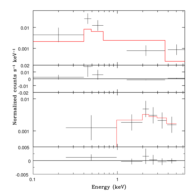
Figure 3: Swift/XRT X-ray spectra of SDSS J124610.75+275615.9 (upper panel) and SDSS J151652.48+395413.4 (lower panel), both taken on 2023-05-03. The best-fit spectral models expressed as $wabs*zwabs*powerlaw$ with a fixed power-law photon index of 2 are overplotted by the red solid lines. The subpanel underneath each spectrum shows the deviations, in units of $\mathrm{counts\ s^{-1}\ keV^{-1}}$ , of the observed data from the best-fit model.

Table 2: Hard X-ray flux in the 2–10 keV energy band.

Object	Mission	Date	$F_{\mathrm{2-10~{}keV}}$	Reference
			($\mathrm{erg\ s^{-1}\ cm^{-2}}$)
(1)	(2)	(3)	(4)	(5)
SDSS J124610.75+275615.9	ROSAT	1990-1991	$(1.9\pm 0.4)\times 10^{-13}$	Zimmermann et al. (2001)
	Swift	2023-05-03	$(1.6\pm 0.9)\times 10^{-13}$	This work
SDSS J151652.48+395413.4	XMM-Newton	2014-08-13	$(2.3\pm 1.2)\times 10^{-12}$	XMM-SSC (2018)
	Swift	2023-05-03	$(9.9\pm 6.7)\times 10^{-13}$	This work

5.4 Estimation of Black Hole Mass and Eddington Ratio

Columns (9) and (10) in Table 1 list the estimated $M_{\mathrm{BH}}$ and $L_{\mathrm{bol}}/L_{\mathrm{Edd}}$, respectively. Thanks to the well-established calibrated relationships based on AGN single-epoch spectra (e.g., Kaspi et al. 2000, 2005; Wu et al. 2004; Peterson & Bentz 2006; Marziani & Sulentic 2012; Du et al. 2014, 2015; Peterson 2014; Wang et al. 2014), the black hole virial mass ($M_{\mathrm{BH}}$) and Eddington ratio ($L_{\mathrm{bol}}/L_{\mathrm{Edd}}$, where $L_{\mathrm{Edd}}=1.5\times 10^{38}\,(M_{\mathrm{BH}}/{\it M}_{\odot})\,\mathrm{erg\,s^{-1}}$ is the Eddington luminosity, Eq. 3.16 in Netzer (2013)) can be estimated in terms of the modeled H$\alpha$ broad emission line through the traditional method described by Wang et al. (2020a).

Briefly, $M_{\mathrm{BH}}$ can be estimated by the calibration (Greene & Ho 2007)

$$\small M_{\mathrm{BH}}=3.0\times 10^{6}\bigg{(}\frac{L_{\mathrm{H\alpha}}}{10^{42}\ \mathrm{erg\ s^{-1}}}\bigg{)}^{0.45}\bigg{(}\frac{\mathrm{FWHM_{H\alpha}}}{1000\ \mathrm{km\ s^{-1}}}\bigg{)}^{2}\ {\rm M}_{\odot}$$ (1)

and $L_{\mathrm{bol}}/L_{\mathrm{Edd}}$ through a bolometric correction of $L_{\mathrm{bol}}=9\lambda L_{\lambda}(5100\,{\rm\AA})$ (e.g., Kaspi et al. 2000), where (Greene & Ho 2005)

$$\lambda L_{\lambda}(5100\,{\rm\AA})=2.4\times 10^{43}\bigg{(}\frac{L_{\mathrm{H\alpha}}}{10^{42}\,\mathrm{erg\,s^{-1}}}\bigg{)}^{0.86}\ \mathrm{erg\,s^{-1}}\,.$$ (2)

In deriving the intrinsic broad H$\alpha$ line luminosity $L_{\mathrm{H\alpha}}$ obtained at different epochs, the measured broad H$\alpha$ line fluxes of individual objects are first scaled by a factor determined by equaling the total [O III] $\lambda$5007 line flux to that of the SDSS DR16 spectrum, which is given by Wang (2015). The intrinsic extinction is then corrected from the narrow-line flux ratio $\mathrm{H\alpha/H\beta}$ by assuming the Balmer decrement of standard Case B recombination and a Galactic extinction curve with $R_{V}=3.1$. Being dominated by the calibration scatter, the uncertainties of $M_{\mathrm{BH}}$ and $L_{\mathrm{bol}}/L_{\mathrm{Edd}}$ are $\sim 0.2$ dex and $\sim 65$% (or 0.28 dex), respectively. $L_{\mathrm{bol}}/L_{\mathrm{Edd}}$ is instead estimated from their unabsorbed X-ray 2–10 keV luminosity for the “turn-off” state of two objects, SDSS J124610.75+275615.9 and SDSS J151652.48+395413.4, by adopting a bolometric correction of $L_{\mathrm{bol}}=16L_{\mathrm{2-10~{}keV}}$.

5.5 Stellar Population of the Hosts of the New CL-AGNs

It is well known that both the 4000 Å break [$D_{\rm n}(4000)$] and the equivalent width (EW) of the H$\delta$ absorption due to A-type stars ($\mathrm{H\delta_{A}}$) are widely used as reliable age indicators in AGN host galaxies until a few Gyr after a starburst (e.g., Kauffmann et al. 2003; Heckman et al. 2004; Kewley et al. 2006; Kauffmann & Heckman 2009; Wild et al. 2010; Wang & Wei 2008, 2010; Wang et al. 2013; Wang 2015), although both indices are sensitive to metallicity in very old stellar populations. The $D_{\rm n}(4000)$ is defined as (Balogh et al. 1999; Bruzual 1983)

$$D_{\rm n}(4000)=\frac{\int_{4000}^{4100}f_{\lambda}d\lambda}{\int_{3850}^{3950}f_{\lambda}d\lambda}\,.$$ (3)

The index H$\delta_{\mathrm{A}}$ is defined as (Worthey & Ottaviani 1997)

$$\mathrm{H\delta_{A}}=(4122.25–4083.50)\bigg{(}1-\frac{F_{I}}{F_{c}}\bigg{)}\ \mathrm{\AA}$$ (4)

where $F_{I}$ is the flux within the feature bandpass of $\lambda\lambda$4083.50–4122.25, and $F_{c}$ the flux of the pseudo continuum evaluated in the two beside regions: blue $\lambda\lambda$4041.60–4079.75 and red $\lambda\lambda$4128.50–4161.00.

Columns (11) ans (12) of Table 1 list the values of both $D_{\rm n}(4000)$ and H$\delta_{\mathrm{A}}$ that are measured from the modeled starlight component by Wang (2015). Combining the uncertainties due to both measurements in duplicate observations (Wang et al. 2011) and AGN continuum removal (Wang 2015), the typical uncertainties of $D_{\rm n}(4000)$ and H$\delta_{\mathrm{A}}$ are estimated to be $\sim 0.04$ and $\sim 0.4$Å, respectively.

5.6 Statistics

5.6.1 SMBH Accretion

Figure 4 shows the distributions of CL-AGNs in the $L_{\mathrm{bol}}$ vs. $M_{\mathrm{BH}}$ (left panels) and $L_{\mathrm{bol}}$ vs. $L_{\mathrm{bol}}/L_{\mathrm{Edd}}$ (right panels) diagrams, after combining the 9 CL “partially obscured” AGNs identified in this study and the CL-AGNs studied and compiled by Wang et al. (2019, see references therein). The comparison samples shown by different symbols and colors are (1) the SDSS DR7 quasars with $z<0.5$ (Shen et al. 2011), (2) the SDSS DR3 narrow-line Seyfert 1 galaxies (NLS1s) given by Zhou et al. (2006), (3) the Swift/BAT AGN sample with a spectral type classification by Winter et al. (2012), and (4) the SDSS intermediate-type Seyfert galaxies studied by Wang (2015). In the figure, the upper two panels correspond to the “turn-on” state, and the lower two panels to the “turn-off” state.

Two facts can be gleaned from the figure. First, compared to the parent sample (i.e., the 170 SDSS “partially obscured” AGNs studied by Wang (2015), the magenta points in Figure 4), one can see from the upper two panels that the “partially obscured” CL-AGNs identified by us tend to be biased against both high $L_{\mathrm{bol}}$ and high $L_{\mathrm{bol}}/L_{\mathrm{Edd}}$ as claimed previously for luminous quasars (e.g., MacLeod et al. 2019; Wang et al. 2019; Frederick et al. 2019; Jin et al. 2022). Second, SDSS J143016.03+230844.2 shows Balmer emission-line profiles that are typical of a Type I AGN at its “turn-on” state with high $L_{\mathrm{bol}}=8.6\times 10^{45}\ \mathrm{erg\ s^{-1}}$ and $L_{\mathrm{bol}}/L_{\mathrm{Edd}}=0.1$, reinforcing our previous claim that there are two kinds of origins of intermediate-type AGNs: one to the well-accepted orientation effect and the other to an intrinsic change of accretion rate (Wang et al. 2019).

Figure 4: Distributions of the CL-AGNs on the $L_{\mathrm{bol}}$–$M_{\mathrm{BH}}$ (left panels) and $L_{\mathrm{bol}}$–$L_{\mathrm{bol}}/L_{\mathrm{Edd}}$ (right panels) diagrams, after combining the 9 new “partially obscured” CL-AGNs (denoted by the solid circles) identified in this study and the 26 previously identified CL-AGNs (denoted by the open squares) complied by Wang et al. (2019). The “turn-on” and “turn-off” states are displayed in the upper and lower rows, respectively. The underlying comparison samples are described as follows. Red crosses, quasars with $z<0.5$ taken from the value-added SDSS DR7 quasar catalog (Shen et al. 2011); green crosses, the SDSS DR3 NLS1 catalog established by Zhou et al. (2006); and magenta crosses, the SDSS DR7 intermediate-type AGNs studied by Wang (2015). The Swift/BAT AGN sample of Winter et al. (2012) is shown by the cyan, yellow, and blue crosses for Seyfert 1, 1.2, and 1.5 galaxies, respectively.

5.6.2 Host Galaxies

The $D_{\rm n}(4000)$ index measured by Wang (2015) ranges from 1.38 to 1.83 for the 9 “partially obscured” CL-AGNs. With a determined standard deviation of 0.15, the average and median values of $D_{\rm n}(4000)$ are 1.58 and 1.59, respectively. A comparison of the cumulative distribution of $D_{\rm n}(4000)$ is presented in Figure 5. A one-side Kolmogrov-Smirnov test returns a result that the distributions of the 9 CL-AGNs and of the parent sample (i.e., the 170 “partially obscured” AGNs studied by Wang (2015)) have a maximum distance of 0.40, which corresponds to a discrepancy with a probability of 0.961. The figure and the corresponding statistics suggest that the CL-AGNs identified in the current study are clearly biased against a young stellar population, and tend to be associated with an intermediate-age stellar population, although a larger sample of CL-AGNs with direct measurements of their host galaxies is needed to confirm these claims at a higher significance level. A value of $D_{\rm n}(4000)=1.4$–1.6 is, in fact, usually adopted as a threshold for separating young and old stellar populations (e.g., Kauffmann et al. 2003). The revealed association with an intermediate-age stellar population roughly agrees with the results recently reported by Liu et al. (2021) and Jin et al. (2022). Liu et al. (2021) point out that the local CL-AGNs tend to reside in galaxies located in the “green valley,” rather than in blue host galaxies, where the average and median $D_{\rm n}(4000)$ values are 1.47 and 1.46, respectively. The corresponding standard deviation of $D_{\rm n}(4000)$ is 0.21. In addition, based on stellar-population synthesis on 26 “turn-off” CL-AGNs, Jin et al. (2022) proposed that CL-AGNs are mainly characterized by intermediate-age stellar populations.

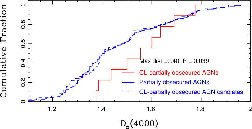
Figure 5: A comparison of the distributions of $D_{\rm n}(4000)$ index. The distribution of the 9 “partially obscured” CL-AGNs is denoted by the red solid line. The blue dashed and blue solid lines show the distribution of the 59 “partially obscured” CL-AGN candidates that are selected according to their variability in the MIR band and the distribution of the total 170 intermediate-type AGNs from which the candidates are selected.

As an additional test, Figure 6 shows the H$\delta_{\mathrm{A}}$ versus $D_{\rm n}(4000)$ plot, after combining the local CL-AGNs identified in this study and the ones quoted from literature. The values of both $D_{\rm n}(4000)$ and H$\delta_{\mathrm{A}}$ of 30 local CL-AGNs are reported in Table 3 in Liu et al. (2021). For the 17 CL-AGNs recently identified in Lopez-Navas et al. (2023), the corresponding Lick indices are obtained from the value-added MPA/JHU catalog (Kauffmann et al. 2003; Heckman & Kauffmann 2006), in which the contamination caused by emission lines has been removed. One can see from the figure that the enlarged sample reinforces the trend that CL-AGNs are associated with an intermediate-aged stellar population.

Figure 6: $D_{\rm n}(4000)-\mathrm{H}\delta_{\mathrm{A}}$ plane for local CL-AGNs (see the main text for the details of the used samples). The underlying density contours (the dashed black heavy lines) show the distribution of $\sim 80,000$ Seyfert 2 galaxies extracted from the MPA/JHU value-added catalog (e.g., Kauffmann et al. 2003; Heckman & Kauffmann 2006). The solid line marks the stellar population evolution locus of the single-stellar population model with solar metallicity, and the dot-dashed line the model with exponentially decreasing star formation rate $\psi(t)\propto e^{-(t/\mathrm{4Gyr})}$.

6 Discussion

Through a follow-up spectroscopy program on the MIR variability-selected SDSS “partially obscured” AGNs, we identified 9 CL-AGNs whose spectral types have changed during past $\sim 15$–20 yr from a parent sample of 59 candidates, which leads to a CL-AGN identification rate of 15%, suggesting that variability in the MIR band is quite useful in searching for and studying the CL phenomenon. Taking into account the parent sample of 170 “partially obscured” AGNs, the CL-AGN fraction is determined to be no less than 5%. This number is much larger than the previously claimed CL-AGN fraction of 0.007–0.11% (e.g., Yang et al. 2018; Yu et al. 2020). In addition, it is interesting that our spectroscopic campaign returns a “turn-on” over “turn-off” ratio of 5:4 that is quite close to 1. Miniutti et al. (2019) argued a connection between CL-AGNs and the rarely discovered X-ray quasiperiodic eruptions (QPE) from SMBHs that predict similar numbers of “turn-on” and “turn-off” CL states according to the symmetric light-curve profile of the eruptions, although the physical origin of the SMBH’s QPE is still an open question.

Subsequent spectral analysis of the “partially obscured” CL-AGNs enables us to reinforce the previous claims that CL-AGNs tend to be biased against both high $L_{\mathrm{bol}}$ and high $L_{\mathrm{bol}}/L_{\mathrm{Edd}}$, and toward an intermediate-age stellar population.

Figure 7 shows that the Keck follow-up spectrum with weak broad H$\alpha$ emission allows us to identify SDSS J151652.48+295413.4 as a new repeat CL-AGNs with a rapid “turn-on” timescale of $\sim 2$ yr. The repeat CL phenomenon is further supported by the X-ray emission level assessed from our new Swift/XRT observation. The X-ray emission is close to that given by the ROSAT survey and leads to $L/L_{\mathrm{Edd}}=0.032$, comparable to the value estimated in the “turn-on” state. Up to now, there have been only eight confirmed repeat CL-AGNs: Mrk 590, Mrk 1018, NGC 1566, NGC 4151, NGC 7603, Fairall 9, 3C 390.3, and UGC 3223 (Marin et al. 2019; Parker et al. 2019; Wang et al. 2020; Mathur et al. 2018). With $M_{\mathrm{BH}}=3.7\times 10^{7}\,{\rm M}_{\odot}$, the timescale of a typical TDE is predicted to be $\Delta t=0.35(M_{\mathrm{BH}}/10^{7}\,{\rm M}_{\odot})^{1/2}(M_{\star}/{\rm M}_{\odot})^{-1}(R_{\star}/{\rm R}_{\odot})^{3/2}\approx 1$ yr (e.g., Rees 1988; Lodato & Rossi 2011, and references therein) for the object, where $M_{\star}$ and $R_{\star}$ are respectively the mass and radius of the disrupted star. Although this prediction is comparable to the “turn-on” timescale revealed in the object, it is difficult for the TDE scenario to explain the repeat CL phenomenon identified in the object, because the TDE rate is expected to be as low as one event every $10^{4}$–$10^{5}$ yr per galaxy (e.g., Gezari et al. 2008; Donley et al. 2002; van Velzen et al. 2014).

Figure 7: A comparison of the line-profile modeling in the H$\alpha$ region of SDSS J151652.48+295413.4. The spectra obtained by SDSS, Shane 3 m, and Keck II 10 m telescopes at different epochs are displayed from left to right. In the modeling of the Keck spectrum, the narrow H$\alpha$ emission line is produced from the profile of the adjacent [N II] $\lambda$6583 emission line by a fixed line flux ratio of 0.9 determined from the SDSS spectrum, because the narrow H$\alpha$ emission line falls in the 12 Å chip gap that is ignored in our modeling. Symbols are the same as in Figure 2.

6.1 Physical Origin of the CL Phenomenon

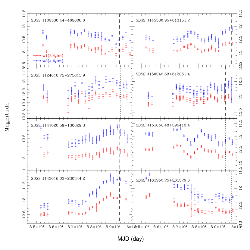
Figure 8: WISE MIR light curves of the 8 “partially obscured” CL-AGNs. Each light curve is binned by averaging the measurements within one day. In each panel, the vertical black lines mark the epochs of our optical spectra, where the long-dashed line corresponds to a “turn-on” state and the short-dashed one to a “turn-off” state.

The MIR light curves of the “partially obscured” CL-AGNs identified in this study are shown in Figure 8, in which the $w1$ (3.4 $\mu$m) and $w2$ (4.6 $\mu$m) values are taken from the Wide-field Infrared Survey Explorer (WISE and NEOWISE-R; Wright et al. 2010; Mainzer et al. 2014). Table 3 compares the relative MIR brightness offsets $\delta w$ at the epoch of our spectroscopy with the identified CL status. The relative offset is defined as $\delta w=(w-\langle w\rangle)/\Delta w$, where $\langle w\rangle$ is the mean brightness and $\Delta w$ the photometric error, respectively. A positive $\delta w$ denotes a MIR brightness fainter than the mean brightness, and a negative one a brighter MIR brightness. Although the epochs of the SDSS DR16 spectra are not covered by the WISE survey, one can see from the table that the CL status revealed by our follow-up spectra is generally related to the $w1$ and $w2$ brightness: a “turn-on” status corresponds to an MIR brightening, and a ‘turn-off” status to an MIR dimming, except SDSS J102530.44+462808.6 and SDSS J124610.75+275615.9. A close inspection of the light curves of both objects shows that their CL status are related with the light curve trends at the corresponding spectroscopic epochs: the “turn-on” phenomenon occurs during the MIR brightening process, and the “turn-off” phenomenon during the MIR dimming process.

Table 3: MIR brightness versus CL status

Object	MJD	$\delta w1$	$\delta w2$	CL status
	(day)
(1)	(2)	(3)	(4)	(5)
J075244.20+455657.4	57428	+1.8	+3.9	off
J102530.44+462808.6	59345	+0.9	+2.0	on
J124610.75+275615.9	59407	$-0.1$	$-0.4$	off
J141020.59+130829.3	59359	$-0.8$	$-1.2$	on
J143016.03+230344.2	59345	$-6.3$	$-7.2$	on
J145536.95+013151.2	59407	$-2.5$	$-2.1$	on
J150240.63+612851.4	59407	$-0.9$	$-0.6$	on
J151652.48+395413.4	59405	+1.0	+2.3	off
J161950.25+261329.6	59724	+0.8	+1.5	off

The dependence of CL status on MIR brightness is consistent with the expectation of the accretion-rate enhancement scenario of the CL phenomenon (e.g., Sheng et al. 2017; Stern et al. 2018; Wang et al. 2019, 2020, 2021; Yang et al. 2018; Lopez-Navas et al. 2022, 2023). In addition to their MIR variation, the spectropolarimetry performed by Hutsemekers et al. (2019) shows that CL-AGNs in the “turn-off” state typically have polarization below 1%, implying that the clumpy obscuration scenario is unlikely to explain the disappearance of the broad emission lines.

The fact that CL-AGNs tend to be biased against high $L_{\mathrm{bol}}$ and high $L_{\mathrm{bol}}/L_{\mathrm{Edd}}$ therefore motivates some authors to argue that the CL phenomenon could be understood by the disk-wind broad-line region (BLR) models previously proposed by Elitzur & Ho (2009) and Nicastro (2000). On the one hand, in the Elitzur & Ho (2009) model, because the mass-outflow rate scales with $L$ as $L^{1/4}$, an observable BLR cannot be sustained below a certain luminosity, $L\approx 5\times 10^{39}(M_{\mathrm{BH}}/10^{7}~{}{\rm M}_{\odot})^{2/3}\,\mathrm{erg\,s^{-1}}$, which corresponds to a critical value of $L_{\mathrm{bol}}/L_{\mathrm{Edd}}\approx 10^{-6}$ (Elitzur & Shlosman 2006).

On the other hand, a much higher critical value of $L_{\mathrm{bol}}/L_{\mathrm{Edd}}\approx 2$–3 $\times 10^{-3}$ has been proposed for $M_{\mathrm{BH}}$ within a range of $10^{7-8}~{}{\rm M}_{\odot}$ by Nicastro (2000), in which the appearance or disappearance of the BLR depends on a critical radius of the accretion disk where the power deposited into the vertical outflow is the maximum value. One would argue against this scenario by being aware of the fact that, as shown in Figure 3 and Table 1, the calculated $L_{\mathrm{bol}}/L_{\mathrm{Edd}}$ at the “turn-off” state is usually higher than the above critical value by an order of magnitude. This problem can be easily resolved since the reported $L_{\mathrm{bol}}/L_{\mathrm{Edd}}$ at the “turn-off” state is usually estimated from the weakened broad Balmer emission lines. In fact, the X-ray inferred $L_{\mathrm{bol}}/L_{\mathrm{Edd}}$ is estimated to be $\sim 2\times 10^{-3}$ and $\sim 1\times 10^{-3}$ for SDSS J075244.20+455657.4 (Wang et al. 2022) and SDSS J151652.48+395413.4 (this study), respectively, at their “turn-off” state with a disappeared classic BLR. In addition, our X-ray observation of the CL-AGN UGC 3223 shows that its $L_{\mathrm{bol}}/L_{\mathrm{Edd}}$ was as low as $\sim 2\times 10^{-4}$ when the broad Balmer emission lines disappeared completely (Wang et al. 2020b, and see Ai et al. (2020) for other cases with $L_{\mathrm{bol}}$ and $L_{\mathrm{bol}}/L_{\mathrm{Edd}}$ inferred from X-rays).

In the disk-wind model, a thermally unstable radiation-pressure-dominated disk region is required for the existence of a BLR, which implies that the thermal timescale is typical of the CL phenomenon. This timescale is, in fact, able to account for the observed variations of order 10–20 yr, especially the $\sim 2$ yr rapid “turn-on” process observed in SDSS J151652.48+395413.4. The evolutionary $\alpha$-disk model developed by Siemiginowska et al. (1996), in fact, predicts

$$\small t_{\mathrm{th}}\approx\frac{1}{\alpha\Omega_{\mathrm{K}}}\\ =2.7\bigg{(}\frac{\alpha}{0.1}\bigg{)}^{-1}\bigg{(}\frac{r}{10^{16}\,\mathrm{cm}}\bigg{)}^{3/2}\bigg{(}\frac{M_{\mathrm{BH}}}{10^{8}~{}{\rm M}_{\odot}}\bigg{)}^{-1/2}\mathrm{yr},$$ (5)

which leads to a variability timescale of 3–8 yr for the 9 “partially obscured” AGNs, when the fiducial values of “viscosity parameter” $\alpha=0.1$ and $r=10^{16}~{}\mathrm{cm}$ and the estimated $M_{\mathrm{BH}}$ are adopted. Additionally, a shorter variability timescale can be obtained either by introducing a narrow unstable zone (Sniegowska et al. 2020), or by involving an accretion disk elevated by a magnetic field (e.g., Ross et al. 2018; Stern et al. 2018; Dexter & Begelman 2019), which is supported by recent numerical simulations carried out by Pan et al. (2021).

On the contrary, the classical viscous radial inflow is not a plausible scenario for the observed CL phenomenon. The viscous timescale of a viscous radial inflow can be estimated as (e.g., Shakura & Sunyaev 1973; Krolik 1999; LaMassa et al. 2015; Gezari et al. 2017)

$$\scriptsize t_{\mathrm{infl}}=6.5\bigg{(}\frac{\alpha}{0.1}\bigg{)}^{-1}\bigg{(}\frac{L/L_{\mathrm{Edd}}}{0.1}\bigg{)}^{-2}\bigg{(}\frac{\eta}{0.1}\bigg{)}^{2}\bigg{(}\frac{r}{r_{g}}\bigg{)}^{7/2}\bigg{(}\frac{M_{\mathrm{BH}}}{10^{8}~{}{\rm M}_{\odot}}\bigg{)}~{}\mathrm{yr}\,,$$ (6)

where $\eta$ is the efficiency of converting potential energy to radiation and $r_{g}$ is the gravitational radius in units of $GM/c^{2}$. Taking the fiducial values of $\alpha=\eta=0.1$, the viscous timescale is estimated to be $10^{3-5}$ yr, when $r\approx(50$–100)$r_{g}$ is adopted to account for the outer disk producing optical emission. However, Feng et al. (2021b) propose that the inflow timescale can be significantly reduced in a magnetic accretion disk-outflow model by magnetic outflows.

With increasing cases of identified CL-AGNs, a few other possible models have been proposed recently to understand the CL phenomenon. For instance, the theoretical study by Wang & Bon (2020) suggests that CL-AGNs could be triggered by close binaries of SMBHs with a high eccentricity. A tidal torque on the mini-disk of each SMBH can either squeeze or expand the disk, resulting in a spectral type transition cycle determined by the orbital period. The authors argue that this scenario is able to explain the highly asymmetric and double-peaked broad-line profiles observed in some CL-AGNs (e.g., Storchi-Bergmann et al. 2017).

6.2 Implication from the Intermediate-Age Stellar Populations

Although no significant difference between the host galaxies of CL-AGNs and NCL-AGNs has been reported by some studies in recent years (e.g., Charlton et al. 2019; Yu et al. 2020; Dodd et al. 2021), our spectroscopic campaign on “partially obscured” CL-AGNs and direct measurements of stellar populations allow us to suggest that CL-AGNs tend to be dominated by intermediate-age populations, roughly consistent with Liu et al. (2021) and Jin et al. (2022).

Given the inferred intermediate-age stellar population and the concept of coevolution between SMBH and host galaxy (see Heckman & Kauffmann 2011, Heckman & Best 2014 for a review), we propose that CL-AGNs are AGNs at a specific evolutionary stage. Figure 9 marks the 9 “partially obscured” CL-AGNs, along with other CL-AGNs identified and complied in previous studies (Lopez-Navas et al. 2022; Liu et al. 2021 and references therein), on the $D_{\rm n}(4000)$–$L_{\mathrm{bol}}/L_{\mathrm{Edd}}$ diagram. There were, in fact, a series of studies that show a strong relationship between $L_{\mathrm{bol}}/L_{\mathrm{Edd}}$ and $D_{\rm n}(4000)$ for local AGNs (Wang 2015 and references therein). The relationship suggests a coevolution between SMBH growth and host galaxy wherein the SMBH resides: $L_{\mathrm{bol}}/L_{\mathrm{Edd}}$ decreases as the young stellar population continuously ages (e.g., Kewley et al. 2006; Wang et al. 2006, 2013; Wang & Wei 2008, 2010; Wang 2015). It is clearly that the local CL-AGNs closely follow the $D_{\rm n}(4000)$–$L_{\mathrm{bol}}/L_{\mathrm{Edd}}$ sequence, and tend to mainly occupy the middle of the sequence simply due to their associated intermediate-aged stellar populations, which implies that CL is a special phenomenon occurring only in evolved AGNs in the context of the coevolution of SMBHs and their host galaxies.

By analyzing the distribution of $L_{\mathrm{bol}}/L_{\mathrm{Edd}}$ as a function of $M_{\mathrm{BH}}$ and properties of the host galaxies for a large sample of local Seyfert 2 galaxies surveyed by SDSS, Kauffmann & Heckman (2009) proposed that there are two distinct regimes of SMBH accretion. On the one hand, the growth of SMBHs associated with a young central stellar population and significant star formation is less dependent on the central stellar population of the galaxy. The plentiful cold gas supply can guarantee a steady inward fueling flow of cold gas (i.e., “feast fueling”). One the other hand, for the SMBHs associated with an old central stellar population, the time-averaged mass growth rate is proportional to the mass of the bulge of the host galaxy (i.e., “famine fueling”). This dependence could be understood if, when the cold gas in a reservoir is consumed, the SMBHs are fed by slow stellar winds generated by evolved stars or by inward mass transport triggered by either minor mergers or multiple collisions of cold-gas clumps in the intergalactic medium (e.g., Kauffmann & Heckman 2009; Davies et al. 2007, 2014; Pizzolato & Soker 2005; Gaspari et al. 2013).

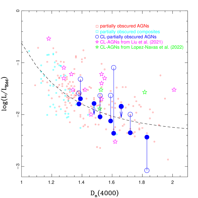
Figure 9: $L_{\mathrm{bol}}/L_{\mathrm{Edd}}$ plotted as a function of stellar population age index $D_{\rm n}(4000)$. The 9 “partially obscured” CL-AGNs identified by us are shown by the solid and open blue circles for the “turn-off” and “turn-on” states, respectively. The other CL-AGNs (at “turn-on” state) compiled in Liu et al. (2021 and references therein) and identified in Lopez-Navas et al. (2022) are displayed by the open stars in magenta and green, respectively. The small red and cyan open squares are the local “partially obscured” Seyfert galaxies and composite galaxies studied by Wang (2015), respectively. The dashed line is the best-fit nonlinear relationship to these “partially obscured” AGNs.

Given the inferred stellar population and the concept of coevolution between SMBH and host galaxy, here we propose that CL-AGNs are probably at a transition between the feast and famine SMBH fueling stages that are profiled by Kauffmann & Heckman (2009). The authors, in fact, indicate that a transition between the aforementioned two SMBH accretion regimes occurs at $D_{\rm n}(4000)=1.5$–1.8, comparable to the measured average value and standard deviation of $D_{\rm n}(4000)$ of the CL-AGNs focused in the current study. At the transition, the cold gas in the reservoir has been almost exhausted by steady inward fueling flow; thereafter, episodic fueling is expected when the fueling is contributed by slow stellar winds of evolved stars, especially those on the asymptotic giant branch, or by chaotic accretion (e.g., King & Pringle 2006, 2007). The proposed particular evolutionary stage of CL-AGNs is supported by recent other studies. On the one hand, from the view of host galaxies, besides the studies of direct stellar populations mentioned above, Dodd et al. (2021) indicate that CL-AGNs tend to reside in high-density pseudobulges located in the so-called “green valley” that is believed to be a transition region between active star-forming galaxies and inactive elliptical galaxies owing to the quenching of AGNs. On the other hand, from the view of SMBH accretion, the MIR Eddington ratio of CL-AGNs is found to be in accord with a transition between a Shakura-Sunyaev disk (Shakura & Sunyaev 1973) and radiatively inefficient accretion flow (Lyu et al. 2022). By comparing CL-AGNs and different types of AGNs, Liu et al. (2021) suggest that CL-AGNs are possible at a specific evolutionary stage with $L_{\mathrm{bol}}/L_{\mathrm{Edd}}\approx 0.1$, since the objects show a transition between the positive and negative $\Gamma–L_{\mathrm{X}}/L_{\mathrm{Edd}}$ correlation in the CL phenomenon.

7 Conclusions

We study the physics of CL-AGNs from the perspective of the coevolution of AGNs and their host galaxies. By focusing on the local “partially obscured” AGNs, our follow-up spectroscopy and detailed analysis of these spectra allow us to arrive at following conclusions.

1. Nine new “partially obscured” CL-AGNs are identified from a sample of 59 candidates that are selected according to their variability in the MIR band.

2. The host galaxies of the identified “partially obscured” CL-AGNs are biased against young stellar populations, and tend to be dominated by intermediate-age stellar populations, consistent with the results recently reported by Liu et al. (2021) and Jin et al. (2022). This population motivates us to propose that CL-AGNs are probably AGNs at a specific evolutionary stage, going from a plentiful supply of cold gas to fueling by the slow stellar winds of evolved stars — that is, at a transition stage from “feast” to “famine” SMBH fueling. The validation of the evolutionary-stage specificity of CL-AGNs requires larger samples of CL-AGNs with directly measured host-galaxy properties. Future studies using such samples would illuminate the relationship between CL-AGN behavior and host-galaxy properties, allowing us to gain deeper insights into the unique evolutionary mechanisms of these objects.

3. We reinforce the claims that CL-AGNs tend to be biased against a high $L_{\mathrm{bol}}/L_{\mathrm{Edd}}$ and a high $L_{\mathrm{bol}}$, implying that the disk-wind BLR model is a plausible explanation of the CL phenomenon.

References

- Ai et al. (2020) Ai, Y. L., Dou, L. M., Yang, C. W., et al. 2020, ApJ, 890, 29
- Antonucci (1993) Antonucci, R. R. J. 1993, ARA&A, 31, 473
- Arnaud (1996) Arnaud, K. A. 1996, ASPC, 101, 17
- Balogh et al. (1999) Balogh, M.L. et al. 1999, ApJ, 527, 54
- Bentz et al. (2013) Bentz, M. C., Denney, K. D., Grier, C. J., et al. 2013, ApJ, 767, 149
- Blanchard et al. (2017) Blanchard, P. K., Nicholl, M., Berger, E., et al. 2017, ApJ, 843, 106
- Boroson (2005) Boroson, T. A. 2005, AJ, 130, 381
- Bowen & Vaughan (1973) Bowen, I. S., & Vaughan, A. H., Jr. 1973, ApOpt, 12, 1430
- Bruhweiler & Verner (2008) Bruhweiler, F., & Verner, E. 2008, ApJ, 675, 83
- Bruzual (1983) Bruzual, A.G. 1983, ApJ, 273, 105
- Bruzual & Charlot (2003) Bruzual, G., & Charlot, S. 2003, MNRAS, 344, 1000
- Cardelli et al. (1989) Cardelli, J. A., Clayton, G. C., & Mathis, J. S. 1989, ApJ, 345, 245
- Charlton et al. (2019) Charlton, P. J. L., Ruan, J. J., Haggard, D., et al. 2019, ApJ, 876, 75
- Cooper et al. (2012) Cooper, M. C., Newman, J. A., Davis, M., Finkbeiner, D. P., & Gerke, B. F. 2012, spec2d, ASCL, 1203.003
- Davies et al. (2017) Davies, R. I., Hicks, E. K. S., Erwin, P., et al. 2017, MNRAS, 466, 4917
- Davies et al. (2014) Davies, R. I., Maciejewski, W., Hicks, E. K. S., et al. 2014, ApJ, 792, 101
- Dexter & Begelamn (2019) Dexter, J., & Begelman, M. C. 2019, MNRAS, 483, L17
- Dietrich et al. (2002) Dietrich, M., Hamann, F., Shields, J. C., et al. 2002, ApJ, 581, 912
- Dimitrijevic et al. (2007) Dimitrijevic, M. S., Popovic, L. C., Kovacevic, J., Dacic, M., & Ilic, D. 2007, MNRAS, 374, 1181
- Dodd et al. (2021) Dodd, S. A., Law-Smith, J. A. P., Auchettl, K., et al. 2021, ApJ, 907, 21
- Donley et al. (2002) Donley, J. L., Brandt, W. N., Eracleous, M., & Boller, T. 2002, AJ, 124, 1308
- Du et al. (2015) Du, P., Hu, C., Lu, K. X., et al. 2015, ApJ, 806, 22
- Du et al. (2014) Du, P., Wang, J. M., Hu, C., et al. 2014, MNRAS, 438, 2828
- Elitzur (2012) Elitzur, M., 2012, ApJ, 747, 33
- Elitzur & Ho (2009) Elitzur, M., & Ho, L. C. 2009, ApJ, 701, 91
- Elitzur et al. (2014) Elitzur, M., Ho, L. C., & Trump, J. R. 2014, MNRAS, 438, 3340
- Elitzur & Shlosman (2006) Elitzur, M., & Shlosman, I. 2006, ApJ, 648, 101
- Faber et al. (2003) Faber, S. M., Phillips, A. C., Kibrick, R. I., et al. 2003, SPIE, 4841, 1657
- Feng et al. (2021a) Feng, H. C., Hu, C., Li, S. S., et al. 2021a, ApJ, 909, 18
- Feng et al. (2021b) Feng, J., Cao, X., Li, J. W., & Gu, W. M. 2021b, ApJ, 916, 61
- Filippenko (1982) Filippenko, A. V. 1982, PASP, 94, 715
- Francis et al. (1992) Francis, P. J., Hewett, P. C., Foltz, C. B., & Chaffee, F.H. 1992, ApJ, 398, 476
- Frederick et al. (2019) Frederick, S., Gezari, S., Graham, M. J., et al. 2019, ApJ, 883, 31
- Gaspari et al. (2013) Gaspari, M., Ruszkowski, M., & Oh, S. P. 2013, MNRAS, 432, 3401
- Gezari et al. (2008) Gezari, S., Basa, S., Martin, D. C., et al. 2008, ApJ, 676, 944
- Gehrels et al. (2004) Gehrels, N., Chincarini, G., Giommi, P., et al. 2004, ApJ, 611, 1005
- Gezari et al. (2017) Gezari, S., Hung, T., Cenko, S. B., et al. 2017, ApJ, 835, 144
- Guo et al. (2019) Guo, H. X., Sun, M. Y., Liu, X., Wang, T. G., Kong, M. Z., Wang, S., Sheng, Z. F., & He, Z. C. 2019, ApJ, 833, 44
- Graham et al. (2020) Graham, M. J., Ross, N. P., Stern, D., et al. 2020, MNRAS, 491, 4925
- Green et al. (2022) Green, P. J., Pulgarin-Duque, L., Anderson, S. F., et al. 2022, arXiv: astro-ph/220109123
- Greene & Ho (2005) Greene, J. E., & Ho, L. C. 2005, ApJ, 630 ,122
- Greene & Ho (2007) Greene, J. E., & Ho, L. C. 2007, ApJ, 670, 92
- Grimm et al. (2003) Grimm, H. -J., Gilfanov, M., & Sunyaev, R. 2003, MNRAS, 339, 793
- Gunn et al. (2006) Gunn, J. E., Siegmund, W. A., Mannery, E. J., et al. 2006, AJ, 131, 2332
- Haoc et al. (2005) Hao, L., et al. 2005, AJ, 129, 1795
- Harrison et al. (2014) Harrison, C. M., Alexander, D. M., Mullaney, J. R., & Swinbank, A. M. 2014, MNRAS, 441, 3306
- Heckman (1980) Heckman, T. M. 1980, A&A, 87, 152
- Heckman & Best (2014) Heckman, T. M., & Best, P. N. 2014, ARA&A, 52, 589
- Heckman & Kauffmann (2006) Heckman, T. M., & Kauffmann, G. 2006, New A Rev., 50, 677
- Heckman & Kauffmann (2011) Heckman, T. M., & Kauffmann, G. 2011, Science, 333, 182
- Heckman et al. (2004) Heckman, T. M., Kauffmann, G., Brinchmann, J., Charlot, S., Tremonti, C., & White, S. D. M. 2004, ApJ, 613, 109
- Hon et al. (2020) Hon, W. J., Webster, R., & Wolf, C. 2020, MNRAS, 497, 192
- Hon et al. (2022) Hon, W. J., Wolf, C., Onken, C. A., Webster, R., & Auchettl, K. 2022, MNRAS, 511, 54
- Husemann et al. (2016) Husemann, B., Urrutia, T., Tremblay, G. R., et al. 2016, A&A, 593, L9
- Hutsemekers et al. (2019) Hutsemekers D., Agis Gonzalez B., Marin F., Sluse D., Ramos Almeida C., Acosta Pulido J.-A., 2019, A&A, 625, A54
- Jarvela et al. (2017) Jarvela, E., Lahteenmaki, A., Lietzen, H., Poudel, A., Heinamaki, P., & Einasto, M. 2017, A&A, 606, 9
- Jin et al. (2022) Jin, J. J., Wu, X. B., & Feng, X. T. 2022, ApJ, 926, 184
- Kalberla et al. (2005) Kalberla, P. M. W., Burton, W. B., Hartmann, D., et al. 2005, A&A, 440, 775
- Kaspi et al. (2005) Kaspi, S., Maoz, D., Netzer, H., et al. 2005, ApJ, 629, 61
- Kaspi et al. (2000) Kaspi, S., Smith, P. S., Netzer, H., et al. 2000, ApJ, 533, 631
- Kauffmann & Heckman (2009) Kauffmann, G., & Heckman, T. M. 2009, MNRAS, 397, 135
- Kauffmann et al. (2003) Kauffmann, G., Heckman, T. M., White, S. D. M., et al. 2003, MNRAS, 341, 33
- Kewley et al. (2006) Kewley, L. J., Groves, B., Kauffmann, G., & Heckman, T. M. 2006, MNRAS, 372, 961
- King & Pringle (2006) King, A. R., & Pringle, J. E. 2006, MNRAS, 373, L90
- King & Pringle (2007) King, A. R., & Pringle, J. E. 2007, MNRAS, 377, L25
- Kollatschny et al. (2020) Kollatschny, W., Grupe, D., Parker, M. L., et al. 2020, A&A, 638, 91
- Kollatschny et al. (2018) Kollatschny, W., Ochmann, M. W., Zetzl, M., Haas, M., Chelouche, D., Kaspi, S., Pozo Nuñez, F., & Grupe, D. 2018, A&A, 619, 168
- Kollmeier et al. (2017) Kollmeier, J. A., Zasowski, G., Rix, H. W., et al. 2017, arXiv: astro-ph/171103234
- Kormendy et al. (2011) Kormendy, J., Bender, R., & Cornell, M. E. 2011, Nature, 469, 374
- Kriss (1994) Kriss, G. 1994, in ASP Conf. Ser. 61, Astronomical Data Analysis Software and Systems III, ed. D. R. Crabtree, R. J. Hanisch, & J. Barnes (San Fransisco, CA: ASP), 437
- Krolik (1999) Krolik, J. H. 1999, Active Galactic Nuclei: From the Central Black Hole to the Galactic Environment (Princeton University Press: Princeton, NJ)
- LaMassa et al. (2015) LaMassa, S. M., Cales, S., Moran, E. C., et al. 2015, ApJ, 800, 144
- Lawrence (2018) Lawrence, A. 2018, Nature Astronomy, 2, 102
- Liu et al. (2021) Liu, W. J., Lira, P., Yao, S., Xu, D. W., Wang, J., Dong, X. B., & Martínez-Palomera, J. 2021, ApJ, 915, 63
- Lodato & Rossi (2011) Lodato, G., & Rossi, E. M. 2011, MNRAS, 410, 359
- López-Navas et al. (2022) López-Navas, E., Martínez-Aldama, M. L., Bernal, S., et al. 2022, MNRAS, 513, L57
- López-Navas et al. (2023) López-Navas, E., Sánchez-Sáez, P., Arévalo, P., et al. 2023, MNRAS, 524, 188
- Lyke et l. (2020) Lyke, B. W., Higley, A. N., McLane, J. N., et al. 2020, ApJS, 250., 8
- Lyu et al. (2022) Lyu, B., Wu, Q., Yan, Z., et al. 2022, ApJ, 927, 227
- MacLeod et al. (2019) MacLeod, C. L., Green, P. J., Anderson, S. F., et al. 2019, ApJ, 874, 8
- MacLeod et al. (2010) MacLeod, C. L., Ivezic, Z., Kochanek, C. S., et al. 2010, ApJ, 721, 1014
- MacLeod et al. (2016) MacLeod, C. L., Ross, N. P., Lawrence, A., et al. 2016, MNRAS, 457, 389
- Mainzer et al. (2014) Mainzer, A., Bauer, J., Cutri, R. M., et al. 2014, ApJ, 792, 30
- Marin et al. (2019) Marin, F., Hutsemekers, D., & Agis Gonzalez, B. 2019, proceedings of the 2019’s annual conference of the SF2A , arXiv/astro-ph:1909.02801
- Malkan & Sargent (1982) Malkan, M. A., & Sargent, W. L. W. 1982, ApJ, 254, 22
- Marinucci et al. (2016) Marinucci, A., Bianchi, S., Nicastro, F., Matt, G., & Goulding, A. D. 2012, ApJ, 748, 130
- Marziani & Sulentic (2012) Marziani, P., & Sulentic, J. W. 2012, NewAR, 56, 49
- Massey et al. (1988) Massey, P., Strobel, K., Barnes, J. V., et al. 1988, ApJ, 328, 315
- Mathur (2000) Mathur, S. 2000, MNRAS, 314, 17
- Mathur et al. (2018) Mathur, S., Denney, K. D., Gupta, A., et al. 2018, ApJ, 886, 123
- Mathur et al. (2012) Mathur, S., Fields, D., Peterson, B. M., & Grupe, D. 2012, ApJ, 754, 146
- McElroy et al. (2016) McElroy, R. E., Husemann, B., Croom, S. M., et al. 2016, A&A, 593, L8
- Merloni et al. (2015) Merloni, A., Dwelly, T., Salvato, M., et al. 2015, MNRAS, 452, 69
- Miller & Stone (1994) Miller, J. S., & Stone, R. P. S. 1994, Lick Obs. Tech. Rep. 66 (Santa Cruz, CA: Lick Observatory)
- Miniutti et al. (2019) Miniutti, G., Saxton, R. D., Giustini, M., et al. 2019, Nature, 573, 381
- Nagoshi et al. (2021) Nagoshi, S., Iwamuro, F., Wada, K., & Saito, T. 2021, PASJ, 73, 122
- Newman et al. (2013) Newman, J. A., Cooper, M. C., Davis, M., et al. 2013, ApJS, 208, 5
- Netzer (2013) Netzer, H. 2013, The Physics and Evolution of Active Galactic Nuclei, by Hagai Netzer, Cambridge, UK: Cambridge University Press, 2013
- Nicastro (2000) Nicastro, F. 2000, ApJ, 530, 65
- Oke et al. (1995) Oke, J. B., Cohen, J. G., Carr, M., et al. 1995, PASP, 107, 375
- Orban de Xivry et al. (2011) Orban de Xivry, G., Davies, R., Schartmann, M., Komossa, S., Marconi, A., Hicks, E., Engel, H., & Tacconi, L. 2011, MNRAS, 417, 2721
- Pan et al. (2021) Pan, X., Li, S. -L., & Cao, X. 2021, arXiv:astro-ph/2103:00828, accetped by ApJ
- Parker et al. (2016) Parker, M. L., Komossa, S., Kollatschny, W., et al. 2016, MNRAS, 461, 1927
- Parker et al. (2019) Parker, M. L., Schartel, N., Grupe, D., et al. 2019, MNRAS, 483, L88
- Perez-Montero & Diaz (2003) Perez-Montero, E., & Diaz, A. I. 2013, MNRAS, 346, 105
- Perley (2019) Perley, D. A. 2019, PASP, 131h4503P
- Peterson (2014) Peterson, B. M. 2014, SSRv, 183, 253
- Peterson & Bentz (2006) Peterson, B. M., & Bentz, M. C. 2006, NewAR, 50, 769
- Peterson et al. (2000) Peterson, B. M., McHardy, I. M., Wilkes, B. J., et al. 2000, ApJ, 542, 161
- Pizzolato & Soker (2005) Pizzolato, F., & Soker, N. 2005, ApJ, 632, 821
- Rees (1988) Rees, M. J. 1988, Nature, 333, 523
- Ricci & Trakhtenbrot (2022) Ricci, C., & Trakhtenbrot, B. 2022, arXiv: astro-ph/221105132
- Risaliti et al. (2009) Risaliti, G., Salvati, M., Elvis, M., et al. 2009, MNRAS, 393, L1
- Ross et al. (2018) Ross, N. P., Ford, K. E. S., Graham, M., et al. 2018, MNRAS, 480, 4468
- Ruan et al. (2016) Ruan, J. J., Anderson, S. F., Cales, S. L., et al. 2016, ApJ, 826, 188
- Ruan et al. (2019) Ruan, J. J., Anderson, S. F., Eracleous, M., Green, P. J., Haggard, D., MacLeod, C. L. Runnoe, J. C., & Sobolewska, M. A. 2019, ApJ, 883, 76
- Runnoe et al. (2016) Runnoe, J. C., Cales, S., Ruan, J. J., et al. 2016, MNRAS, 455, 1691
- Sani et al. (2010) Sani, E., Lutz, D., Risaliti, G., et al. 2010, MNRAS, 403, 124
- Shakura & Sunyaev (1973) Shakura, N. I., & Sunyaev, R. A. 1973, A&A, 24, 337
- Shapovalova et al. (2010) Shapovalova, A. I., Popovic, L. C., Burenkov, A. N., et al. 2010, A&A, 509, 106
- Shappee et al. (2014) Shappee, B. J., Prieto, J. L., Grupe, D., et al. 2014, ApJ, 788, 48
- Scharwachter et al. (2017) Scharwachter, J., Husemann, B., Busch, G., Komossa, S., & Dopita, M. A. 2017, ApJ, 848, 35
- Schlegel & Finkbeiner (2011) Schlafly, E. F., & Finkbeiner, D. P. 2011, ApJ, 737, 103
- Schlegel et al. (1998) Schlegel, D., Finkbeiner, D. P., & Davis, M. 1998, ApJ, 500, 525
- Shen et al. (2011) Shen, Y., Richards, G. T., Strauss, M. A., et al. 2011, ApJS, 194, 45
- Sheng et al. (2017) Sheng, Z., Wang, T., Jiang, N., et al. 2017, ApJ, 846, 7
- Sheng et al. (2020) Sheng, Z., Wang, T., Jiang, N., et al. 2020, ApJ, 889, 46
- Siemiginowska et al. (1996) Siemiginowska, A., Czerny, B., & Kostyunin, V. 1996, ApJ, 458, 491
- Smee et al. (2013) Smee, S. A., Gunn, J. E., Uomoto, A., et al. 2013, AJ, 146, 32
- Sniegowska et al. (2020) Sniegowska, M., Czerny, B., Bon, E., & Bon, N. 2020, A&A, 641, 167
- Stern et al. (2018) Stern, D., McKernan, B., Graham, M. J., et al. 2018, ApJ, 864, 27
- Storchi-Bergmann et al. (2017) Storchi-Bergmann, T., Schimoia, J. S., Peterson, B. M., Elvis, M., Denney, K. D., Eracleous, M., & Nemmen, R. S. 2017, ApJ, 835, 236
- Storey & Hummer (1995) Storey, P. J., & Hummer, D. G. 1995, MNRAS, 272, 41
- Strateva et al. (2003) Strateva, I. V., Strauss, M. A., Hao, L., et al. 2003, AJ, 126, 1720
- Tody (1986) Tody, D. 1986, Proc. SPIE, 627, 733
- Tody (1992) Tody, D. 1992, in ASP Conf. Ser. 52, Astronomical Data Analysis Software and Systems II, ed. R. J. Hanisch, R. J. V. Brissenden, & J. Barnes (San Fransisco, CA: ASP), 173
- Trakhtenbrot et al. (2019) Trakhtenbrot, B., Arcavi, I., MacLeod, C. L., et al. 2019, ApJ, 883, 94
- van Velzen & Farrar (2014) van Velzen, S., & Farrar, G. R. 2014, ApJ, 792, 53
- Veron-Cetty et al. (2004) Veron-Cetty, M. -P., Joly, M., & Veron, P. 2004, A&A, 417, 515
- Voges et al. (1999) Voges, W., Aschenbach, B., Boller, T., et al. 1999, A&A, 349, 389
- Wang (2015) Wang, J. 2015, NewA, 37, 15
- Wang et al. (2011) Wang, J., Mao, Y. F., & Wei, J. Y. 2011, ApJ, 741, 50
- Wang & Wei (2008) Wang, J., & Wei, J. Y. 2008, ApJ, 679, 86
- Wang & Wei (2010) Wang, J., & Wei, J. Y. 2010, ApJ, 719, 1157
- Wang et al. (2006) Wang, J., Wei, J. Y., & He, X. T. 2006, ApJ, 638, 106
- Wang et al. (2020a) Wang, J., Xu, D. W., Sun, S. S., Feng, Q. C. Li T. R., Xiao, P. F., & Wei, J. Y. 2020a, AJ, 159, 245
- Wang et al. (2020b) Wang, J., Xu, D. W., & Wei, J. Y. 2020b, ApJ, 901, 1
- Wang et al. (2018) Wang, J., Xu, D. W., & Wei, J. Y. 2018, ApJ, 852, 26
- Wang et al. (2019) Wang, J., Xu, D. W., Wang, Y., Zhang, J. B., Zheng, J., & Wei, J. Y. 2019, ApJ, 887, 15
- Wang et al. (2018) Wang, J., Xu, D. W., & Wei, J. Y. 2018, ApJ, 858, 49
- Wang et al. (2022a) Wang, J., Zheng, W. K., Xu, D. W., Brink, T. G., Filippenko, A. V., Gao, C., Sun, S. S., & Wei, J. Y. 2022, RAA, 22, 015011
- Wang et al. (2013) Wang, J., Zhou, X. L., & Wei, J. Y. 2013, ApJ, 768, 176
- Wang et al. (2014) Wang, J. M., Du, P., Hu, C., et al. 2014, ApJ, 793, 108
- Wang & Bon (2020) Wang, J. -M., & Bon, E. 2020, ApJ, 643, 9
- Wang et la. (2022b) Wang, Y., Jiang, N., Wang, T., et al. 2022b, ApJS, 258, 21
- Wild et al. (2010) Wild, V., Heckman, T. M., & Charlot, S. 2010, MNRAS, 405, 933
- Wild et al. (2007) Wild, V., Kauffmann, G., Heckman, T., et al. 2007, MNRAS, 381, 543
- Winter et al. (2012) Winter, L. M., Veilleux, S., McKernan, B., & Kallman, T. R. 2012, ApJ, 745, 107
- Woo et al. (2017) Woo, J. H., Son, D., & Bae, H. J. 2017, ApJ, 839, 120
- Worthey & Ottaviani (1997) Worthey, G., & Ottaviani, D. L. 1997, ApJS, 111, 377
- Wright et al. (2010) Wright, E. L., Eisenhardt, P. R. M., Mainzer, A. K., et al. 2010, AJ, 140, 1868
- Wu et al. (2004) Wu, X. B., Wang, R., Kong, M. Z., Liu, F. K., & Han, J. L. 2004, A&A, 424, 793
- XMM-SSC (2018) XMM-SSC 2018, VizieR Online Data Catalog: XMM-Newton Slew Survey Source Catalogue, version 2.0
- Yan et al. (2019) Yan, L., Wang, T. G., Jiang, N., et al. 2019, ApJ, 874, 44
- Yang et al. (2018) Yang, Q., Wu, X. B., Fan, X. H., et al. 2018, ApJ, 862, 109
- Yu et al. (2020) Yu, X., Shi, Y., Chen, Y., et al. 2020, MNRAS, 498, 3985
- Zhang et al. (2013) Zhang, K., Wang, T., Gaskell, C. M., & Dong, X. 2013, ApJ, 762, 51
- Zhou et al. (2006) Zhou, H. Y., Wang, T. G., Yuan, W. M., et al. 2006, ApJS, 166, 128
- Zimmermann et al. (2001) Zimmermann, H. -U., Boller, T., Döbereiner, S., & Pietsch, W. 2001, A&A, 378, 30