PivotNet: Vectorized Pivot Learning for End-to-end HD Map Construction

Abstract

Vectorized high-definition map online construction has garnered considerable attention in the field of autonomous driving research. Most existing approaches model changeable map elements using a fixed number of points, or predict local maps in a two-stage autoregressive manner, which may miss essential details and lead to error accumulation. Towards precise map element learning, we propose a simple yet effective architecture named PivotNet, which adopts unified pivot-based map representations and is formulated as a direct set prediction paradigm. Concretely, we first propose a novel Point-to-Line Mask module to encode both the subordinate and geometrical point-line priors in the network. Then, a well-designed Pivot Dynamic Matching module is proposed to model the topology in dynamic point sequences by introducing the concept of sequence matching. Furthermore, to supervise the position and topology of the vectorized point predictions, we propose a Dynamic Vectorized Sequence loss. Extensive experiments and ablations show that PivotNet is remarkably superior to other SOTAs by 5.9 mAP at least. The code will be available soon.

1 Introduction

High-definition map (HD map) is one of the most critical components in many autonomous driving modules, including simulation, localization, and planning. Typical HD map construction relies on manual annotation on lidar point clouds, which is time-consuming and labor-intensive. Recent works explore the map learning problems to reduce the labeling costs [9, 11, 20, 25, 42]. Given data from onboard sensors, map learning aims to construct local map within a predefined bird’s-eye-view (BEV) range.

Most existing works view the map construction as a semantic learning problem [9, 20, 25, 42]. They represent a map within certain range as an evenly spaced field and predict the class label for each grid, generating a rasterized map. However, there are obvious limitations of rasterized representation in map learning. First, rasterized maps are composed of dense semantic pixels that contain redundant information, requiring large amounts of memory and transmission bandwidth, especially if the map extent is large. Second, the rasterized representation assumes the independence of map grids, which ignores the geometric relationship between and within map elements. Third, complex post-processing [11] is required to obtain vectorized maps for downstream tasks, which brings additional computation, time consumption, and accumulated errors.

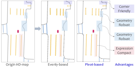
Figure 1: Illustration of our motivation for pivot-based vectorization. Given an original HD map example from nuScenes, there are two different ways to construct a vectorized map, i.e. evenly-based and pivot-based. Comparison shows that pivot-based vectorization is more corner-friendly, geometry-robust, and expression-compact. Circles on the lines denote the real vectorization GT.

To address the limitations of current semantic learning methods, there have been proposals for generating vectorized representations in an end-to-end manner. One such method is MapTR [15], which uses a fixed number of points to represent a map element, regardless of its shape complexity. However, this approach has two drawbacks. First, the evenly-based representation contains redundant points that have little effect on the geometry. Second, representing a dynamically shaped line with a fixed number of points may miss essential details in map elements, resulting in information loss, particularly for rounded corners and right angles (Fig.1). Therefore, to learn an accurate and compact representation, we model a map element as an ordered list of pivotal points, which is expression compact, corner friendly, and geometry robust. However, the pivot-based representation brings new challenges due to the dynamic number of the pivot points within different map elements. Previous work [18] has utilized a coarse-to-fine framework and autoregressive decoding to address these challenges, but the autoregressive nature can lead to long inference time and accumulated errors. Towards these issues, we propose PivotNet, which accurately models map elements through pivot-based representation in a set prediction framework.

The framework of PivotNet is depicted in Fig. 2, which presents an architecture consisting of four primary modules: the camera feature extractor, BEV feature decoder, line-aware point decoder, and pivotal point predictor. The surrounding multi-view images from onboard cameras are fed into the camera feature extractor, which generates camera view features. Next, the image features are aggregated and transformed into a unified BEV feature through the BEV feature decoder. The lane-aware point decoder then extracts line-aware point features. Finally, the pivotal point predictor removes collinear points and predicts a flexible yet compact pivot-based representation.

To be concrete, we first propose a point-to-line mask module for the line-aware point decoder, which encodes both the subordinate and geometric point-line relation through a line-aware mask. Secondly, we further design a pivot dynamic matching module, which models the connection in pivotal point sequences by introducing the concept of sequence matching. A custom sequence matching algorithm is further devised to enhance the time efficiency. Lastly, we propose a novel dynamic vectorized sequence loss to supervise the position and topology of the vectorized point predictions, through both pivot and collinear point supervision. By formulating the task as a sparse set prediction problem and leveraging an end-to-end sequence matching based bipartite matching loss, we present a method that generates precise yet compact vectorized representations without requiring any post-processing.

The contributions of the paper are threefold:

• We present PivotNet, an end-to-end framework for precise yet compact HD map construction via pivot-based vectorization.

• We innovatively introduce point-to-line mask module, pivot dynamic matching module, and dynamic vectorized sequence loss for accurate map element modeling.

• PivotNet exhibits remarkable superiority over state of the arts (SOTAs) on existing benchmarks, indicating the effectiveness of our approach.

2 Related Works

2.1 Semantic map learning

HD map encompasses intricate details that transcend the scope of standard maps, which amplifies the challenge of precise annotations. The conventional process of map construction hinges upon the utilization of LiDAR sensors. This intricate pipeline encompasses stages such as data collection, point cloud registration [10, 21, 32, 33, 41, 43] and manual annotation. To curtail the labeling expenses and enhance overall efficiency, map learning techniques have been introduced. These methods aim to extract pertinent map elements from various on-board sensors, such as cameras and LiDAR sensors [9, 20, 11]. Most approaches generates semantic BEV map representations only. To transform the image features to the BEV space, VPN [25] utilize a multilayer perceptron to learn the mapping between camera views and the BEV. LSS [26] and BEVDet [8] bridge the view gap based on the depth distribution estimation. With the prevalent DETR [2] paradigm, recent methods adopt BEV queries and encode the geometry prior in the attention mechanism in Transformer [3, 14, 42, 39]. To obtain vectorized map for downstream tasks, HDMapNet [11] first produce semantic map and then groups pixel-wise segmentation results in the post-processing. Instead of adopting the semantic first and vectorization later pipeline, PivotNet learns the vectorized map representation in an end-to-end manner.

2.2 Vectorized HD Map Construction

To avoid time-consuming post-processing, recent works explore vectorized map learning methods [15, 18] to obtain compact vectorized map in an end-to-end manner. It is challenging to model the topology between and within map elements due to the various geometric shape and complexity. MapTR [15] models a map element using a fixed number of points, which results in information loss, especially for the rounded corners and the right-angles. VectorMapNet [18] utilizes a coarse-to-fine architecture with an autoregressive network, which leads to long inference time and possible accumulated errors. Different from the existing works [15, 18], PivotNet models a map element using a dynamic number of pivotal points and adopts a set prediction paradigm, which preserves map details while avoiding the drawbacks of [18].

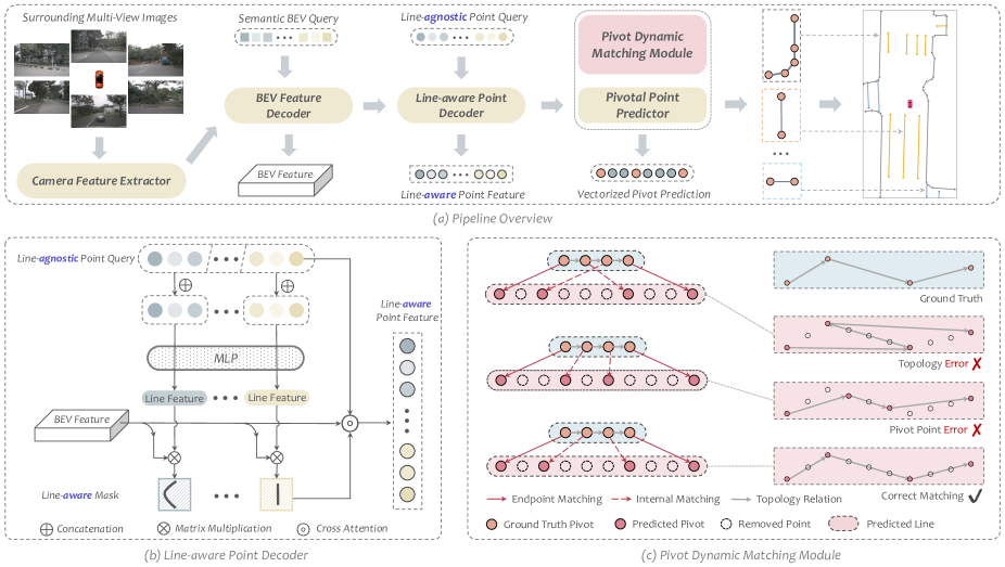
Figure 2: An overview of the proposed PivotNet. The top row is the architecture pipeline of our model, containing four primary components for extracting progressively richer information, which takes the RGB images as inputs and generates flexible and compact vectorized representation without any post-processing. The bottom row illustrates detailed structures of the line-aware point decoder which decodes the map elements from the BEV feature, and the pivot dynamic matching module which enables end-to-end sequence learning.

2.3 Topology Modeling of Map Elements

There are many works to model map elements in a sparse manner. Some methods generate map elements in a recurrent way. HDMapGen[23] generates synthetic HD map by using a hierarchical graph. Global graph with important points are first generated using a recurrent attention network and lane details are then generated using MLPs. VectorMapNet [18] adopts a coarse-to-fine scheme, which predicts coarse shape first and generates points on element in a recurrent way. The recurrent nature of these works makes them time-consuming and hard to train. Other methods formulate map element detection as a keypoint estimation and association problem [28, 38], which lack geometry relations modeling in point regression and need complex post-processing to group keypoints. Some anchor-based approaches [12, 34] utilize the lane shape prior via special design on the anchor. There are also approaches that model the lanes as parameterized curves, such as polynomial curve [16, 36] and Bezier curve [6, 17, 27]. Considering the changeful map elements, we choose the polyline representation. Rather than adopting the two-stage coarse-to-fine [18, 23] or bottom-up [22, 28, 38] design, we model both the point-level and line-level geometries in a uniform manner, and innovatively incorporate point-line prior through line-aware attention masks.

3 Method

We first present the formulation of vectorized HD map modeling with pivot-based representation in Sec.3.1. Then we elaborate on the design of PivotNet in Sec.3.2. Lastly, we present the overall training loss in Sec.3.3.

3.1 Problem Formulation

Our objective is to generate vectorized representations for map elements in urban environments, utilizing data from onboard RGB cameras [11, 15, 18]. We illustrate the problem formulation in Fig. 3. For each map element $\mathcal{L}$, we formulate it as a vectorized sequence $\mathcal{S}$ constructed by $N$ ordered points, where the connection of points is implicitly encoded in the index ordering. As $N$ tends to infinity, $\mathcal{S}$ tends to $\mathcal{L}$, which is formulated as $\displaystyle\lim_{N\to\infty}\mathcal{S}(N)=\mathcal{L}$. To form an efficient and compact representation, we further divide the vectorized sequence $\mathcal{S}$ into a pivotal point sequence $\mathcal{S}^{p}$ and a collinear point sequence $\mathcal{S}^{c}$ by the contribution to the map element shape. The pivotal sequence consists of a list of ordered pivot points that contribute to the overall shape and typically indicate a change in direction in a map element. Given a tolerable error $\epsilon$, $\mathcal{S}^{p}$ is supposed to be a subsequence of $\mathcal{S}$ that satisfies $d(\mathcal{S}^{p},L)<\epsilon$ with the minimum sequence length, where $d(\cdot)$ denotes a distance metric. The collinear point sequence $\mathcal{S}^{c}$ is the complement sequence of $\mathcal{S}^{p}$ and $\mathcal{S}^{c}=\mathcal{S}-\mathcal{S}^{p}$. $\mathcal{S}^{c}$ consists of the points that are collinear to any two adjacent points in $\mathcal{S}^{p}$ and do not significantly contribute to the element shape. We denote the points in $\mathcal{S}^{c}$ as collinear points. Note map elements are often referred to as instances or lines in the next sections.

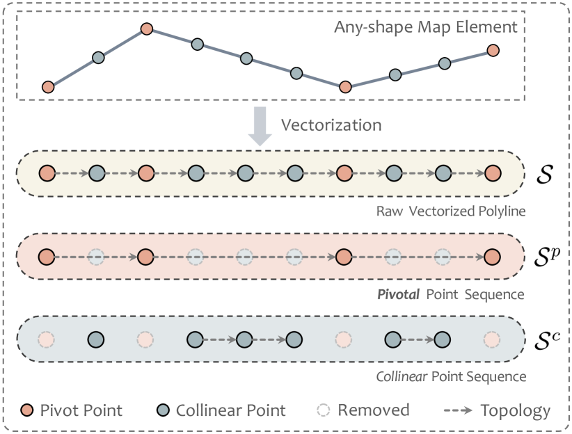
Figure 3: Problem Formulation. An any-shape map element is modeled as a vectorized sequence, which are split into pivotal sequence and collinear sequence. Pivot points are points that contribute to the overall shape and direction of the lines and are necessary to maintain its essential features. Collinear points refer to points that can be safely removed without affecting the line shape.

Preliminary on vectorized HD map modeling. We formulate the map construction task as a set prediction problem. We aim to learn a model that extracts compact information from the onboard cameras and predicts, for each map element, its corresponding pivotal point sequence, which uniquely determines the map element shape and position. Logically, there are three main challenges.

1) Point-Line Relation Modeling. Based on the formulation, a map element is formed by a list of ordered points. For accurate modeling of map elements, it is crucial to encode the point-line relationship prior in the network. In Sec.3.2.2, we propose the Point-to-Line Mask module, which models both the subordinate and geometrical relation in a direct and interpretable manner.

2) Intra-instance Topology Modeling. Vectorization necessitates precise topological relationships between points. For instance, distinct topology with the same point set can represent entirely distinct line shapes (refer to Fig.2 (c)). In Sec.3.2.3, we propose efficient Pivot Dynamic Matching to model and constrain the topology within an instance.

3) Intra-instance Dynamic Point Number Modeling. To achieve compactness in representation, our basic principle is to accurately represent map elements using the fewest possible pivotal points. Therefore, even for the same type of map element, such as a $road$-$boundary$, different instances require a dynamic number of points to achieve precise representation. The proposed pivot dynamic matching approach naturally solves the dynamic number problem through pivotal point classification.

3.2 PivotNet

3.2.1 Architecture Overview.

The overall model architecture is presented in Fig. 2, which consists of four primary components as follows:

Camera Feature Extractor. Given multi-view images from the onboard cameras, a shared backbone network is adopted to extract image features. Then the multi-view image features are concatenated in order as outputs.

BEV Feature Decoder. Following [3, 14], we aggregate and transform the image features into a unified BEV representation via a Transformer-based module, while the deformable attention mechanism is adopted to reduce the computational memory. Specifically, a group of learnable parameters are predefined as BEV queries, where each query represents a grid cell in the BEV plane and only interacts with its regions of interest across camera views. To utilize the geometry prior between camera and BEV features, reference points of each BEV query are determined by the projection of BEV coordinates on the camera views.

Line-aware Point Decoder. We view the vectorized map construction as a set prediction task, and utilize a mask-attention based transformer to decode the lines from the BEV features. Specifically, this module takes the BEV features $F^{b}\in\mathbb{R}^{C\times H^{b}\times W^{b}}$ and a set of learnable point queries $\{Q_{m,n}\}_{m=1,n=1}^{M,N}$, where $Q_{m,n}\in\mathbb{R}^{C}$, and outputs a set of point descriptors $\{D_{m,n}\}_{m=1,n=1}^{M,N}$. Here $M$ is the max number of instances and $N$ is the max number of points in an instance. Each descriptor $D_{m,n}\in\mathbb{R}^{C}$ captures essential positional information and geometrical relationships within and between instances. Moreover, a descriptor $D_{m,n}$ corresponds to a point on the line, and an ordered list composed of descriptors $\{D_{m,n}\}_{n=1}^{N}$ represents a potential map element. To model the point-line relation, we propose a novel Point-to-Line Mask module, which encodes both the subordinate and geometric relation in a straightforward manner with the added benefit of auxiliary supervision.

Pivot Point Head. This module consists of a pivotal point predictor and a pivot dynamic matching module. Given a set of point descriptors $\{D_{m,n}\}_{m=1,n=1}^{M,N}$, a set of point coordinates $\hat{V}=\{\hat{v}_{m,n}\}_{m=1,n=1}^{M,N}$ are first generated via point regression, where $\hat{v}_{m,n}\in\mathbb{R}^{2}$ denotes a point coordinate. We define an ordered point sequence $\hat{\mathcal{S}}=\{\hat{v}_{m,n}\}_{n=1}^{N}$ to represent a map element with index $m$, which contains both pivotal and collinear points. Therefore, to model the sequence order, we propose a novel Pivot Dynamic Matching module for end-to-end sequence learning. Based on the matching results, $\hat{\mathcal{S}}$ is split into a pivotal sequence $\hat{\mathcal{S}}^{p}$ and a collinear sequence $\hat{\mathcal{S}}^{c}$. During inference, the pivotal point predictor identifies the valid map elements and pivotal points, and outputs compact pivot-based representations.

3.2.2 Point-Line Relation Modeling.

As illustrated in Sec.3.2.1, we approach the vectorized map construction as a set prediction task. To accomplish this, we utilize a transformer network [4] with each query representing a point. Yet, this approach poses an inherent challenge. Specifically, in the cross-attention module, there is no clear distinction between inter-instance and intra-instance points, which can result in mixed instances. Thus, it is crucial to encode the point-line relationship in the network to ensure accurate modeling of map elements. There exist both subordinate and geometrical priors between points and lines. The subordinate prior reflects the fact that some points belong to the same line, while others belong to different lines. The geometrical prior states that an ordered list of points contain the necessary information to form a line.

Point-to-Line Mask Module. Previous research on map construction [15] has focused on encoding subordinate priors using hierarchical queries. In this paper, we propose a novel module, called the Point-to-Line Mask module (PLM), that encodes both the subordinate and geometrical relations. The fundamental concept of this module is that a vectorized ordered point sequence is capable of constructing a map element. Based on this concept, we enforce the point queries of the same instance to learn a shared line-aware attention mask. The line mask is then incorporated in the cross-attention layer, implicitly encoding the subordinate relation through shared or different line-level masks. Additionally, the geometry relation is explicitly constrained through supervision on the line-aware mask.

As is shown in Fig.2 (b), point queries $\{Q_{m,n}\}_{n=1}^{N}$ of the same instance with index $m$ are concatenated and fed into a multilayer perceptron, resulting in the instance-level line feature $I_{m}\in\mathbb{R}^{C}$. Then the line feature $I_{m}$ and the BEV feature map ${F}^{b}\in\mathbb{R}^{C\times H^{b}\times W^{b}}$ are multiplied to obtain the line-aware mask $\mathcal{M}_{m}\in\mathbb{R}^{H^{b}\times W^{b}}$. This mask is subsequently used in the cross-attention layer, along with the BEV feature and line-agnostic point queries, to produce line-aware point features. Notably, the line-aware mask effectively constrains the attention region of point queries to within the corresponding foreground map element region. Moreover, each unique attention mask is responsible for all the point queries of the same instance, which further enhances the subordinate prior encoding.

Line-aware Loss. To ensure meaningful line features and constrain the geometrical relations, we introduce the line-aware loss $\mathcal{L}_{LA}$, which is formulated as follows:

$$\mathcal{L}_{LA}=\mathcal{L}_{bce}(\hat{M}_{line},M_{line})+\mathcal{L}_{dice}(\hat{M}_{line},M_{line}).$$ (1)

Here $\hat{M}_{line}$ denotes the line-aware mask feature and $M_{line}$ denotes the segmentation ground truth. $\mathcal{L}_{bce}$ and $\mathcal{L}_{dice}$ are the binary cross-entropy loss and dice loss [24] respectively.

3.2.3 Vectorized Pivot Learning.

Pivot Dynamic Matching. The arbitrary shape and dynamic point number of map elements bring challenges to topology modeling within instances. To address these issues, we propose Pivot Dynamic Matching (PDM), which models the connection in dynamic point sequence by introducing the concept of sequence matching. A custom matching algorithm is further proposed to enhance time efficiency.

We consider the point matching problem between a predicted sequence $\hat{\mathcal{S}}=\{\hat{v}_{n}\}_{n=1}^{N}$ and a ground truth sequence $\mathcal{S}^{p}=\{{v}_{n}\}_{n=1}^{T}$. Here $N$ is the predefined max number of points in a line prediction and $T$ is the length of a ground truth sequence. $N$ is fixed while $T$ is dynamic depending on the map element shape. The instance index $m$ is omitted here for readability. $\hat{\mathcal{S}}$ contains both the pivot and collinear points, while $\mathcal{S}^{p}$ contains pivot points only. We denote a $T$-combination of the prediction $\hat{\mathcal{S}}$ sorted by point index as $\beta$. Apparently, if there are no constraints, the total number of unique $\beta$ is $C_{N}^{T}$. Examples of pivotal point matching are shown in Fig.2 (c). Let’s denote the $\beta(n)$-th point in the sequence prediction as $\hat{v}_{\beta(n)}$. Given $\hat{\mathcal{S}}$, $\mathcal{S}^{p}$ and a combination $\beta$, we define the sequence matching cost as,

$$\mathcal{L}_{{match}}(\hat{\mathcal{S}},\mathcal{S}^{p},\beta)=\frac{1}{T}{\sum_{n=1}^{T}||{v}_{n}-\hat{v}_{\beta^{(}n)}||_{1}},$$ (2)

where $||\cdot||_{1}$ denotes $L_{1}$ norm. The proposed PDM searches for the optimal $\beta^{*}$ with the lowest sequence matching cost:

$$\beta^{*}=\mathop{\arg\min}\limits_{\beta}\mathcal{L}_{match}(\hat{\mathcal{S}},\mathcal{S}^{p},\beta),$$ (3)

Based on the matching result, $\hat{\mathcal{S}}$ is split into a pivot sequence $\hat{\mathcal{S}}^{p}$ and a collinear sequence $\hat{\mathcal{S}}^{c}$, where $\hat{\mathcal{S}}^{p}=\{\hat{v}_{\beta^{*}(n)}\}_{n=1}^{T}$ and $\hat{\mathcal{S}}^{c}=\hat{\mathcal{S}}-\hat{\mathcal{S}}^{p}$. For predicted lines with distinct point distribution, the optimal $\beta^{*}$ is different, resulting in distinct splits of pivot sequence $\hat{S}^{p}$ and collinear sequence $\hat{S}^{c}$. A brute force solution to find the optimal $\beta^{*}$ is to calculate the sequence matching cost for each $\beta$, leading to $O(C_{N}^{T})$ time complexity. To improve efficiency, we further devise a custom matching algorithm and reduce the time complexity to $O(NT)$. As we treat the entire ordered sequence as a possible map element, a fixed correspondence of endpoints to those of the ground truth is enforced, i.e., $\beta(1)=1$, $\beta(T)=N$. With such design, we are able to adopt the idea of dynamic programming. We use an array $dp$, where $dp[i][j]$ denotes the lowest sequence matching cost between the front-$i$ points in the target sequence and the front-$j$ points in the prediction sequences. Then,

$$dp[i][j]=\mathop{\min}\limits_{k\in[1,j-1]}dp[i-1][k]+||v_{i}-\hat{v}_{j}||_{1}$$ (4)

The base case is $dp[1][1]=||v_{1}-\hat{v}_{1}||_{1}$. The optimal $T$-combination $\beta^{*}$ is obtained during traversal in $dp$, which ends when $i=T,j=N$. We use another array to store the minimum cost during traversal to avoid unnecessary sorting, which is detailed in Supplementary Materials.

Dynamic Vectorized Sequence Loss. To satisfy the problem formulation, we propose a novel Dynamic Vectorized Sequence loss (DVS), which provides meaningful constraints for both the pivotal point sequence $\hat{\mathcal{S}}^{p}$ and the collinear sequence $\hat{\mathcal{S}}^{c}$, as well as the topology of the vectorized point predictions. DVS loss consists of three main parts, including pivotal point supervision, collinear point supervision, and pivot classification loss.

1) Pivotal Point Supervision. Based on the matching result, predicted pivot points in $\hat{S}^{p}$ is in one-to-one correspondence to the ground truth sequence $S^{p}$, and $|\hat{S}^{p}|=|S^{p}|=T$. Pivotal point loss constrains the $L_{1}$ distance between $\hat{\mathcal{S}}^{p}$ and the ground truth sequence $\mathcal{S}^{p}$, which is formulated as:

$$\mathcal{L}_{pp}=\frac{1}{T}{\sum_{n=1}^{T}||\hat{\mathcal{S}}^{p}_{n}-\mathcal{S}^{p}_{n}||_{1}}.$$ (5)

2) Collinear Point Supervision. Based on the formulation, a collinear point in $\hat{\mathcal{S}}^{c}$ is supposed to be collinear to certain adjacent points in $\hat{\mathcal{S}}^{p}$ following the order in $\hat{\mathcal{S}}$. Assume there are $R_{n}$ collinear points between two adjacent pivot points $\hat{\mathcal{S}}^{p}_{n}$ and $\hat{\mathcal{S}}^{p}_{n+1}$, where $1\leq n\leq T-1$, then $|\hat{\mathcal{S}}^{c}|=\sum_{n=1}^{T-1}R_{n}=N-T$. We consider a collinear point $\hat{C}_{n,r}$ between $\hat{\mathcal{S}}^{p}_{n}$ and $\hat{\mathcal{S}}^{p}_{n+1}$ that ranks $r$ among $R_{n}$ collinear points. To ensure the linearity, the target coordinate of $\hat{C}_{n,r}$ is supposed to be:

$$C_{n,r}=(1-\theta_{n,r})S^{p}_{n}+\theta_{n,r}S^{p}_{n+1},$$ (6)

where $\theta_{n,r}$ is a coefficient that controls the relative position and $0<\theta_{n,r}<1$. Larger $\theta_{n,r}$ represents that $C_{n,r}$ is nearer to $S^{p}_{n+1}$ while farther from $S^{p}_{n}$. Therefore, to ensure the ordering of the sequence prediction, $\theta_{n,r}$ is supposed to increase monotonically with $r$. For implementation convenience, we define $\theta_{n,r}=r/(R_{n}+1)$. Then the collinear point loss is formulated as:

$$\mathcal{L}_{cp}=\frac{1}{N-T}\sum_{n=1}^{T-1}\sum_{r=1}^{R_{n}}||\hat{C}_{n,r}-C_{n,r}||_{1}.$$ (7)

3) Pivot Classification Loss. To model the dynamic pivotal point number, a binary cross-entropy loss is adopted to supervise the probability of a predicted point being a pivotal point. Given the probability of each point $\{p_{n}\}_{n=1}^{N}$ in an element prediction, classification loss is formulated as:

$$\mathcal{L}_{cls}=\frac{1}{N}\sum_{n=1}^{N}\mathcal{L}_{bce}(p_{n},\mathds{1}_{\hat{\mathcal{S}}_{n}\in\hat{\mathcal{S}}^{p}}),$$ (8)

where $N$ is the predefined maximum number of points in a map element. $\mathds{1}_{A}$ is an indicator function which returns $1$ if $A$ is true, and returns $0$ otherwise.

Then the DVS loss is formulated as follows:

$$\mathcal{L}_{DVS}=\alpha_{1}\mathcal{L}_{pp}+\alpha_{2}\mathcal{L}_{cp}+\alpha_{3}\mathcal{L}_{cls},$$ (9)

where $\alpha_{1}$, $\alpha_{2}$ and $\alpha_{3}$ denote the weighted factors.

3.3 Training Loss

Auxiliary BEV Supervision. To ensure that BEV features contain necessary map information, we introduce an auxiliary segmentation-based loss for BEV supervision:

$$\mathcal{L}_{BEV}=\mathcal{L}_{bce}(\hat{M}_{bev},M_{bev})+\mathcal{L}_{dice}(\hat{M}_{bev},M_{bev}).$$ (10)

$\hat{M}_{bev}$ is the predicted BEV mask and $M_{bev}$ is the ground truth. $\mathcal{L}_{bce}$ represents the binary cross-entropy loss and $\mathcal{L}_{dice}$ denotes dice loss [24].

Overall Loss. The overall loss is formulated as follows:

$$\mathcal{L}_{TOTAL}=\mathcal{L}_{DVS}+\lambda_{1}\mathcal{L}_{LA}+\lambda_{2}\mathcal{L}_{BEV},$$ (11)

where $\lambda_{1}$ and $\lambda_{2}$ are weighted factors.

Method	BKB	Epoch	AP${}_{\textit{divider}}$	AP${}_{\textit{ped}}$	AP${}_{\textit{boundary}}$	mAP	AP${}_{\textit{divider}}$	AP${}_{\textit{ped}}$	AP${}_{\textit{boundary}}$	mAP	FPS	Params.
			$\{0.2,0.5,1.0\}m$				$\{0.5,1.0,1.5\}m$
LSS [26]	EB0	30	22.9	5.1	24.2	17.4	-	-	-	-	-	-
VPN [25]	EB0	30	22.1	5.2	25.3	17.5	-	-	-	-	-	-
HDMapNet [11]	EB0	30	28.3	7.1	32.6	22.7	-	-	-	-	-	-
‡HDMapNet [11]	EB0	30	17.7‡	13.6‡	32.7‡	21.3‡	23.6‡	24.1‡	43.5‡	31.4‡	0.7‡	69.8M
VectorMapNet [18]	R50	110	27.2†	18.2†	18.4†	21.3†	47.3	36.1	39.3	40.9	1.2†	19.4M
MapTR [15]	R50	24	30.7†	23.2†	28.2†	27.3†	51.5	46.3	53.1	50.3	10.1†	35.9M
PivotNet (Ours)	EB0	24	39.4	32.9	37.1	36.5	55.7	55.1	58.5	56.4	7.7	17.1M
PivotNet (Ours)	R50	24	41.4	34.3	39.8	38.5	56.5	56.2	60.1	57.6	6.7	41.2M
PivotNet (Ours)	SwinT	24	45.0	36.2	41.2	40.8	60.6	59.2	62.2	60.6	5.1	44.8M
PivotNet (Ours)	EB0	30	43.7	34.7	40.2	39.6	59.7	53.9	61.0	58.2	7.7	17.1M
PivotNet (Ours)	R50	30	42.9	34.8	39.3	39.0	58.8	53.8	59.6	57.4	6.7	41.2M
PivotNet (Ours)	SwinT	30	47.6	38.3	43.8	43.3	63.8	58.7	64.9	62.5	5.1	44.8M
PivotNet (Ours)	SwinT	110	53.6	43.4	50.5	49.2	68.0	62.6	69.7	66.8	5.1	44.8M

Table 1: Comparison with SOTAs on nuScenes. The ^† indicates that results are re-evaluated on the tighter threshold setup with their released model checkpoint. And ^‡ represents that the performances are reproduced with their public codes. Results in green and blue shades mean that the pedestrian crossing are modeled with polygon as  [15, 18] and straight lines as  [11]. All mAP are obtained by averaging across three map elements. All numbers in the column of FPS are re-test in the same $2080$Ti GPU device for fair comparison.

4 Experiments

4.1 Experimental Settings

Benchmarks. We evaluate PivotNet on two popular and large-scale datasets, i.e. nuScenes [1] and Argoverse 2 [40]. The nuScenes dataset is annotated with $2$Hz. Each frame contains RGB images from surrounding $6$ cameras, which cover full $360$ degree field of view. There are $1000$ scenes in the dataset, where each scene contains around $40$ frames. The dataset is split to $28K$ frames for training and $6K$ frames for validation. The Argoverse 2 is annotated with $10$Hz. Each frame contains $7$ ring cameras and $2$ stereo cameras. We use images from the ring cameras only. There are $110K$ frames for train and $24K$ frames for validation.

Evaluation Protocol. Following previous methods [11, 15, 18], we consider three categories of map element, namely $lane$-$divider$, $ped$-$crossing$, and $road$-$boundary$ for evaluating HD map construction. Note the prediction map range is defined as $30m$ front and rear and $15m$ left and right of the vehicle. The common average precision (AP) based on Chamfer Distance is adopted as the evaluation metric. We consider AP under three thresholds of $\{0.2,0.5,1.0\}m$ in default, where a prediction is treated as true positive (TP) only if the distance between prediction and ground-truth is less than the specified threshold. Furthermore, evaluation with an easier threshold setting of $\{0.5,1.0,1.5\}m$ is also taken into account in Table 1 for fair comparison.

Implementation Details. We adopt EfficientNet-B0 [35], ResNet50 [7], and SwinTiny [19] as backbones and employ transformer-based architecture as BEV feature extractor and line-aware point decoder, whose number of encoder/decoder layers are set to $4$/$4$ and $0$/$6$ respectively. Moreover, we set the BEV feature size to $64\times 32$ and the max number of point queries to $\{200,50,450\}$ for $lane$-$divider$, $ped$-$crossing$, and $road$-$boundary$, where the max number of instances $M=\{20,25,15\}$ and the max number of points $N=\{10,2,30\}$. Our model is trained on $8$ NVIDIA $2080$Ti GPUs with batch size $1$ per GPU. We use the AdamW [31] optimizer with learning rate $2e^{-4}$ and weight decay $1e^{-4}$. Following the multistep scheduler, the learning rate is decayed by a factor of $0.2$ when training to the schedule of $0.7$ and $0.9$ of total epochs. The weighted factors $\{\alpha_{1},\alpha_{2},\alpha_{3},\lambda_{1},\lambda_{2}\}$ are set to $\{5,2,2,5,3\}$ respectively without fine tune.

Method	BKB	Epoch	AP${}_{\textit{divider}}$	AP${}_{\textit{ped}}$	AP${}_{\textit{boundary}}$	mAP
‡HDMapNet [11]	EB0	6	19.5	9.8	35.9	21.8
‡VectorMapNet [18]	R50	24	33.3	18.3	20.4	24.0
‡MapTR [15]	R50	6	42.2	28.3	33.7	34.8
PivotNet (Ours)	EB0	6	46.4	29.8	42.4	39.5
PivotNet (Ours)	R50	6	47.5	31.3	43.4	40.7
PivotNet (Ours)	SwinT	6	48.0	30.6	44.5	41.0
PivotNet (Ours)	SwinT	10	51.1	36.1	47.8	45.0

Table 2: Comparison with state-of-the-art method on Argoverse 2. The meanings of symbol ^‡ is the same as in Table 1.

4.2 Comparisons with State-of-the-art Methods

Results on nuScenes. In Table 1, we compare the overall evaluation performance of PivotNet with existing SOTAs on nuScenes [1] under different settings. Existing methods use different AP thresholds in evaluation. Note [11] employs the threshold of $\{0.2,0.5,1.0\}m$ while [18] and [15] adopt an easier setting of $\{0.5,1.0,1.5\}m$. Therefore, we evaluate PivotNet with both settings in Table 1 for a fair comparison. Compared to the existing state-of-the-art  [15], we achieve $11.2$ higher mAP with the $\{0.2,0.5,1.0\}m$ setting and ${7.3}$ higher mAP with the $\{0.5,1.0,1.5\}m$ setting. The results of PivotNet with various backbones and training epochs are also provided. The reproduced performances of existing methods [11, 15, 25, 26] are obtained based on the public source code (^‡) and released model checkpoint (^†).

Results on Argoverse 2. Table 2 benchmarks PivotNet on a newly large-scale dataset Argoverse 2 [40] and compares the performance with SOTAs. The methods [11, 15, 18] are reproduced with the public source code and then adapted to the Argoverse 2 benchmark. Note all results in Table 2 are evaluated with the $\{0.2,0.5,1.0\}m$ threshold, and with pedestrian crossings modeled by polygons. As can be seen, PivotNet is superior to the existing SOTA approaches [11] by a considerable margin on Argoverse 2.

# Row	PLM	PDM	AP${}_{\textit{divider}}$	AP${}_{\textit{ped}}$	AP${}_{\textit{boundary}}$	mAP
1	✗	✗	33.8	36.8	32.4	34.4
2	✓	✗	42.3	35.5	34.9	37.6
3	✗	✓	40.6	37.4	39.6	39.2
4	✓	✓	47.6	38.3	43.8	43.3

Table 3: Effectiveness of different modules in PivotNet. All results are conducted on nuScenes with thresholds $\{0.2,0.5,1.0\}m$. PLM denotes the proposed point-to-line mask module and PDM denotes the pivotal dynamic matching.

4.3 Ablation Study

Effectiveness of different modules. We conduct ablations on nuScenes to carefully analyze how much each module contributes to the final performance of PivotNet. Table 3 summarizes all results in great details. Specifically, the first row represents the baseline method, which adopts a vanilla transformer-based point decoder and a classification-based length predictor (as point sequence matcher). As a simple alternative of sequence matching for arbitrary length sequence modeling, the later predicts the number of pivotal points as $k$ and outputs front-$k$ points as the final line. Comparison between row 2 and row 4 shows the effectiveness of dynamic sequence matching, especially on the complex-shaped $road$-$boundary$ with $8.9\%$ higher AP. Comparison between row 3 and row 4 validates the effectiveness of the proposed point-to-line mask module with $4.9\%$ higher mAP. Finally, we integrate the above two modules into baseline and show the final improvements in Row 4.

$\mathcal{L}_{BEV}$	AP${}_{\textit{divider}}$	AP${}_{\textit{ped}}$	AP${}_{\textit{boundary}}$	mAP
✗	44.3	37.4	42.4	41.4
✓	47.6(+3.3)	38.3(+0.9)	43.8(+1.4)	43.3(+1.9)

Table 4: Effectiveness of BEV supervision. All results are conducted on nuScenes with thresholds $\{0.2,0.5,1.0\}m$.

Method	AP${}_{\textit{divider}}$	AP${}_{\textit{ped}}$	AP${}_{\textit{boundary}}$	mAP
Point Query	40.6	37.4	39.6	39.2
Hierarchical Query	37.4(-3.2)	33.1(-4.3)	37.3(-2.3)	35.9(-3.3)
PLM (Ours)	47.6(+7.0)	38.3(+0.9)	43.8(+4.2)	43.3(+4.1)

Table 5: Comparison of point-line relation modeling methods.

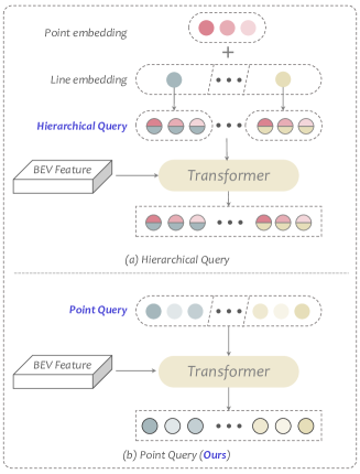
Figure 4: Comparison between hierarchical query and point query design. Hierarchical queries of the same line share the same line embedding and those with the same point index share the same point embedding. Point queries are both line-independent and index-independent.

Effectiveness of BEV loss. Table. 4 shows the effectiveness of BEV supervision. $\mathcal{L}_{bev}$ improves the performance by $1.9\%$ mAP by constraining the BEV features to capture meaningful information within the BEV range.

Discussion of the point-line relation modeling. In Table 5, we compare different methods to model the point-line relation, including the point-to-line mask module (PLM) and the existing methods [15] with hierarchical queries. Row 1 represents the baseline of the line-aware point decoder with no point-line prior, utilizing a vallina mask-attention based transformer [4]. Comparison between row 1 and 2 suggests that the hierarchical query design like [15] is unhelpful to the dynamic sequence modeling. The reason is below. We present the hierarchical queries and the point queries in Fig.4. In the hierarchical query design [15], point queries with the same index share the same point embedding. However, as we model a map element using a dynamic number of points, there is little relation between points with the same index in different line prediction. As illustrated in Sec.3.2.3, the indexes of points selected to form the pivot sequences are various, depending on the point distribution. In short, the hierarchical embedding is index-dependent, which is in conflict with our index-independent problem formulation and may introduce noises about the index information. Therefore, to avoid the index-dependent embedding, we adopt point queries and embed the subordinate and geometrical point-line relation in the attention masks.

Method	mAP0.2m	mAP0.5m	mAP1.0m	mAP1.5m
HDMapNet [11]	11.5	20.8	31.9	38.6
VectorMapNet [18]	1.1(-10.4)	16.6(-4.2)	46.2(+14.3)	64.0(+25.4)
MapTR [15]	2.2(-9.3)	24.7(+3.9)	55.1(+23.2)	70.1(+31.5)
PivotNet (Ours)	13.3(+1.8)	40.8(+20.0)	61.4(+29.5)	70.6(+32.0)

Table 6: Comparison of improvement under different thresholds. Note the mAP is obtained by averaging across three map elements.

Discussion of different AP thresholds. Different threshold setups represent different tolerance degree of the evaluation protocol to model performance. Considering the application of auto-driving, HD map usually requires centimeter-level information, so we argue that the improvement under stricter threshold is more practical. Compared with HDMapNet [11], VectorMapNet [18] and MapTR [15] significantly improves under simple thresholds, e.g. $1.0m$, $1.5m$, but the improvement margin drop rapidly in stricter scenarios, e.g. $0.2m$, $0.5m$. Table 6 shows that no matter which threshold is token, our model always achieves better results, which shows the robustness of our framework.

Layer Num.	AP${}_{\textit{divider}}$	AP${}_{\textit{ped}}$	AP${}_{\textit{boundary}}$	mAP
1	37.8	34.4	36.1	36.1
3	46.7	36.8	41.9	41.8
6	47.6	38.3	43.8	43.3
7	47.1	37.7	42.8	42.6

Table 7: Impact of line-aware point decoder layer number. The gray row represents the setting we use in default.

Impact of line-aware point decoder layer number. The effect of the layer number in line-aware point decoder is evaluated in Table 7. The performance of PivotNet improves with more layer and saturates at layer number of $6$. Therefore, we stack $6$ layers for the decoder.

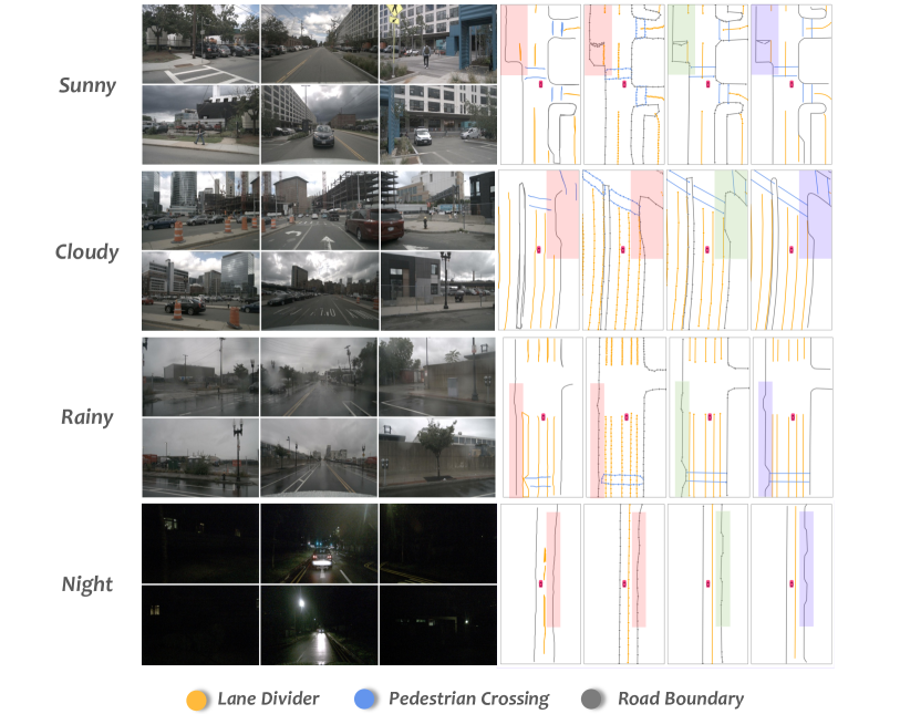
Figure 5: Comparison with SOTAs on qualitative visualization under different weather and lighting conditions, i.e. sunny, cloudy, rainy and night. Each sub-part contains four qualitative results of HDMapNet [11], MapTR [15], PivotNet and GroundTruth respectively. The red and green shades show the differences and alignments with the ground truth in blue area. Please zoom in to see more vectorized point details. Note that we further provide more detailed visualization results in the supplementary material.

Qualitative Analysis. We show the qualitative comparisons with SOTAs in Fig. 5 under various environment conditions.

1) PivotNet vs. HDMapNet. Besides avoiding complex vectorized post-processing, our pivot-based method expresses endpoints more accurately than segmentation-based ones.

2) PivotNet vs. MapTR. Our approach express map shapes, e.g. straight lines, rounded-corners, and right-angles, more smoothly than the method based on uniform-split polylines. Moreover, the PivotNet requires fewer points for modeling.

3) PivotNet vs. GroundTruth. Compared to other methods, our model is robust to various driving scenes and maintains good performance in different environments. Even at night, the map near the vehicle closely matches the ground truth.

Additional ablation Discussions. Due to space limitation, we further provide more extensive ablation studies on encoder/decoder layer number, and predefined instance/point number in Supplementary Materials.

5 Conclusion

This paper focuses on the map construction and view the task as a direct point set prediction problem. We present an end-to-end framework for precise and compact pivot-based HD map construction, which embeds both geometrical and subordinate relations into map elements modeling in a unified manner. By introducing three well-designed modules, i.e. Point-to-Line Mask Module (PLM), Pivot Dynamic Matching (PDM) module, and Dynamic Vectorized Sequence (DVS) loss, the proposed PivotNet reaches SOTA results and provides a new perspective for future research.

Supplementary Material

In this supplementary material, we provide additional details which we could not include in the main paper due to space limitation. Specifically, we provide:

• Detailed illustrations on PivotNet design.

• Additional ablation studies.

• Extensive qualitative visualization results.

Appendix A Detailed illustrations on model design

A.1 Code of the custom matching algorithm

We provide the python code of the custom matching algorithm as follows. The input $cost$ refers to the distance array, where ${cost[i][j]}$ denotes the $L_{1}$ distance between the $i$-th point in the ground truth and the $j$-th point in the line prediction. $dp[i][j]$ denotes the lowest matching cost between the front-$i$ points in the ground truth and the front-$j$ points in the line prediction. $mem\_sort$ stores the minimum cost during traversal to avoid unnecessary sorting. $match\_res1$ and $match\_res2$ store the temporary matching results.

def pivot_dynamic_matching(cost: np.array): A, B = cost.shape assert A ¿= 2 and B ¿= 2,  ”A line should contain two points at least” if A ¿ B: # special case seq_dist = 0 for j in range(B): seq_dist += cost[j][j] combination = list(range(B)) return seq_dist, combination dp = np.ones((A, B)) * np.inf mem_sort = np.ones((A, B)) * np.inf match_res1 = [[] for _in range(B)] match_res2 = [[] for _in range(B)] # initialize for j in range(0, B-A+1): match_res1[j] = [0] mem_sort[0][j] = cost[0][0] if j == 0: dp[0][j] = cost[0][0] # update for i in range(1, A): for j in range(i, B-A + i+1): dp[i][j] = mem_sort[i-1][j-1]  + cost[i][j] if dp[i][j] ¡ mem_sort[i][j-1]: mem_sort[i][j] = dp[i][j] if i ¡ A-1: match_res2[j] = match_res1[j-1] + [j] else: mem_sort[i][j] = mem_sort[i][j-1] if i ¡ A -1: match_res2[j] = match_res2[j-1] if i ¡ A-1: match_res1 = match_res2.copy() match_res2 = [[] for _in range(B)] seq_dist = dp[-1][-1] combination = match_res1[-2] + [B-1] return seq_dist, combination

A.2 Detailed illustrations of notations

Fig.6 illustrates the notations of pivot dynamic matching (PDM) in detail. As stated in Sec.3.2.3, given a ground truth sequence $S^{p}=\{v_{n}\}_{n=1}^{T}$, and a predicted line $\hat{S}=\{\hat{v}_{n}\}_{n=1}^{N}$, PDM searches the optimal T-combination $\beta^{*}$ with the lowest sequence matching cost among all the T-combinations. $T$ is the length of the ground truth sequence, and $N$ is the predefined max number of points in a line prediction. For predicted lines with distinct point distribution, the optimal $\beta^{*}$ is different, resulting in distinct splits of pivot sequence $\hat{S}^{p}$ and collinear sequence $\hat{S}^{c}$. Fig.6 shows examples of $\beta^{*},S^{p},\hat{S},\hat{S}^{p}$ and $\hat{S}^{c}$.

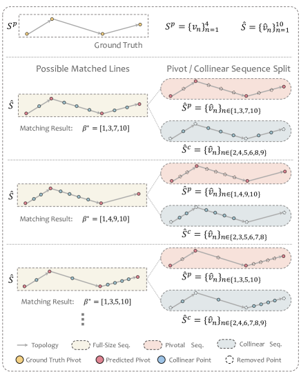
Figure 6: More illustrations of notations in pivot dynamic matching module. $\beta^{*}$ is the optimal $T$-combination for the predicted lines with respect to the ground truth. The figure shows the case where $T=4,N=10$. The ground truth sequence $S^{p}$ contains only pivot points while the predicted sequence $\hat{S}$ contains both pivot points and collinear points. $\hat{S}$ is split into a pivot sequence $\hat{S}^{p}$ and a collinear sequence $\hat{S}^{c}$ based on $\beta^{*}$, which is different for distinct point distribution. Predicted pivot points in $\hat{S}^{p}$ is in one-to-one correspondence to the ground truth sequence $S^{p}$, and $|S^{p}|=|\hat{S}^{p}|=T$, while the number of collinear points $|\hat{S}^{c}|$ is $N-T$.

A.3 Ground-truth pivot point generation

Pivot points in the paper are defined as the points in a map element that contribute to the overall shape and typically indicate a change in direction. Ground-truth pivot point generation can be considered as a polyline simplification problem, which has been studied for years [5, 13, 29, 30, 37]. Given a polyline connected by vertices, polyline simplification aims to find a similar polyline with fewer vertices, which we call pivot points. In this paper, we choose Visvalingam-Whyatt (VW) algorithm [37] to generate ground-truth pivot points. Given an ordered set of points, the importance of each interior point is determined by the area of triangle formed by it and its immediate neighbors. Then the point with the smallest triangle area is obtained. If the area is below the predefined threshold, the point is removed from the set. After that, the triangle area is calculated again to find the most unimportant point. This process is repeated until no triangle area is below the threshold. It is worth noting that the VW algorithm [37] is used for ground truth generation only and can be simply replaced by other pivot point generation methods like [5, 13, 29, 30].

Appendix B Additional ablation studies

B.1 Impact of BEV encoder layer number

The impact of BEV encoder layer number is evaluated in Table 8. The performance of PivotNet improves with more encoder and decoder layers. Even with single encoder and decoder layer, PivotNet achieves satisfying performance, i.e., $36.0\%$ in mAP.

Layer Num.	AP${}_{\textit{divider}}$	AP${}_{\textit{ped}}$	AP${}_{\textit{boundary}}$	mAP
(1, 1)	38.2	33.7	36.0	36.0
(2, 4)	45.5	36.9	42.4	41.6
(4, 2)	46.3	38.2	41.8	42.1
(4, 4)	47.6	38.3	43.8	43.3
(6, 6)	48.0	38.9	45.9	44.3

Table 8: Impact of BEV encoder layer number. The gray row represents the setting we use in default.

B.2 Impact of the maximum instance number

We evaluate the effect of maximum instance number in Table 9. We define the maximum instance number based on the rule that it should be larger than the instance number in typical ground truth. In default, we choose maximum instance number of $(20,25,15)$ for $lane$-$divider$, $ped$-$crossing$, and $road$-$boundary$ respectively. We provide performances with other number settings in Table 9. The performance of PivotNet get saturated when the maximum instance number is set to $(20,25,15)$.

Instance Num.	AP${}_{\textit{divider}}$	AP${}_{\textit{ped}}$	AP${}_{\textit{boundary}}$	mAP
(15, 20, 10)	46.5	37.1	42.8	42.2
(20, 25, 15)	47.6	38.3	43.8	43.3
(30, 30, 30)	47.6	38.9	43.2	43.2

Table 9: Impact of the maximun instance number. The gray row represents the setting we use in default.

B.3 Impact of the maximum pivot point number

The impact of the maximum pivot point number is evaluated in Table 10. The maximum number of pivot points roughly represents the complexity of map elements that PivotNet is able to model. For a certain type of map element, too small maximum number will lead to insufficient modeling capability, yet too large maximum number will increase the learning burden of the model. Therefore, an appropriate value is required for trade-off.

Pivot Point Num.	10	20	30
AP${}_{\textit{divider}}$	47.6	47.5	42.6
Pivot Point Num.	30	50	60
AP${}_{\textit{boundary}}$	43.8	45.4	43.2

Table 10: Impact of the maximum pivot point number.

Appendix C More qualitative visualization results

Fig.7-10 provide extensive visualization results for comparison with SOTA approaches [11, 15] on various environmental conditions. The visualization of HDMapNet [11] is reproduced with its public code, and that of MapTR [15] is generated by its released model checkpoint. Even in challenging road scenarios like intersections and dense roads, PivotNet produces accurate yet compact representations.

We visualize the predictions of the PivotNet with Swin-Tiny [19] backbone on nuScenes. The predictions on different environmental conditions are presented. Even at the most challenging night scenario, the predictions near the vehicle closely match the ground truth (see Fig. 10). Seen from visualization, the modeling of PivotNet is flexible and can describe map elements of arbitrary shape, including line segments, curves, and combinations of them.

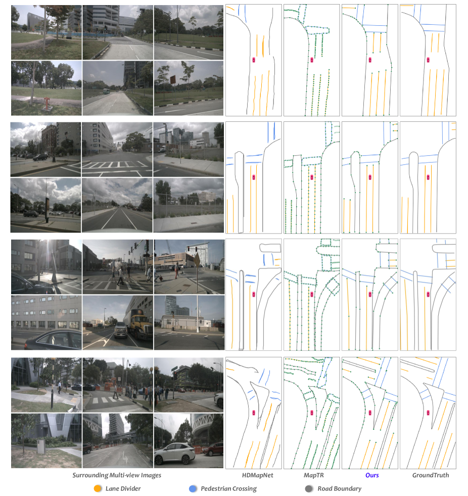
Figure 7: Visualization results under the weather condition of sunny.

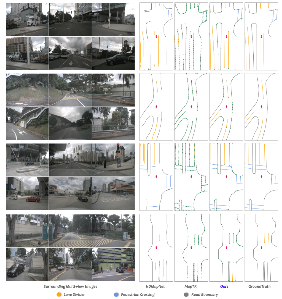
Figure 8: Visualization results under the weather condition of cloudy.

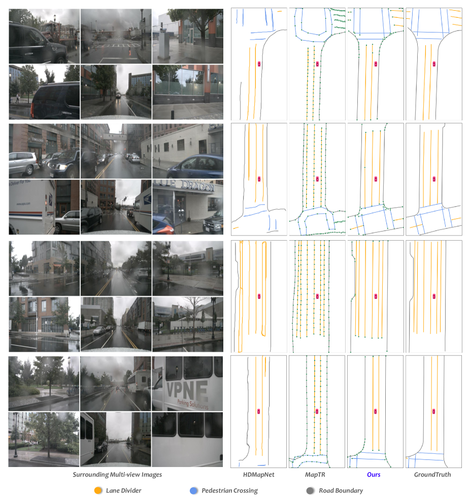
Figure 9: Visualization results under the weather condition of rainy.

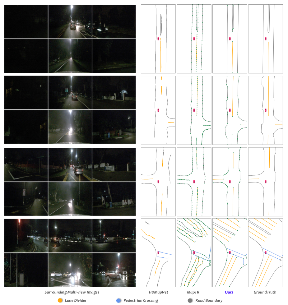
Figure 10: Visualization results under the lighting condition of nighttime.

References

- [1] Holger Caesar, Varun Bankiti, Alex H Lang, Sourabh Vora, Venice Erin Liong, Qiang Xu, Anush Krishnan, Yu Pan, Giancarlo Baldan, and Oscar Beijbom. nuscenes: A multimodal dataset for autonomous driving. In Proceedings of the IEEE/CVF conference on computer vision and pattern recognition, pages 11621–11631, 2020.
- [2] Nicolas Carion, Francisco Massa, Gabriel Synnaeve, Nicolas Usunier, Alexander Kirillov, and Sergey Zagoruyko. End-to-end object detection with transformers. In Andrea Vedaldi, Horst Bischof, Thomas Brox, and Jan-Michael Frahm, editors, Computer Vision - ECCV 2020 - 16th European Conference, Glasgow, UK, August 23-28, 2020, Proceedings, Part I, volume 12346 of Lecture Notes in Computer Science, pages 213–229. Springer, 2020.
- [3] Li Chen, Chonghao Sima, Yang Li, Zehan Zheng, Jiajie Xu, Xiangwei Geng, Hongyang Li, Conghui He, Jianping Shi, Yu Qiao, et al. Persformer: 3d lane detection via perspective transformer and the openlane benchmark. In Computer Vision–ECCV 2022: 17th European Conference, Tel Aviv, Israel, October 23–27, 2022, Proceedings, Part XXXVIII, pages 550–567. Springer, 2022.
- [4] Bowen Cheng, Ishan Misra, Alexander G Schwing, Alexander Kirillov, and Rohit Girdhar. Masked-attention mask transformer for universal image segmentation. In Proceedings of the IEEE/CVF Conference on Computer Vision and Pattern Recognition, pages 1290–1299, 2022.
- [5] David H Douglas and Thomas K Peucker. Algorithms for the reduction of the number of points required to represent a digitized line or its caricature. Cartographica: the international journal for geographic information and geovisualization, 10(2):112–122, 1973.
- [6] Zhengyang Feng, Shaohua Guo, Xin Tan, Ke Xu, Min Wang, and Lizhuang Ma. Rethinking efficient lane detection via curve modeling. In Proceedings of the IEEE/CVF Conference on Computer Vision and Pattern Recognition, pages 17062–17070, 2022.
- [7] Kaiming He, Xiangyu Zhang, Shaoqing Ren, and Jian Sun. Deep residual learning for image recognition. In Proceedings of the IEEE conference on computer vision and pattern recognition, pages 770–778, 2016.
- [8] Junjie Huang, Guan Huang, Zheng Zhu, Ye Yun, and Dalong Du. Bevdet: High-performance multi-camera 3d object detection in bird-eye-view. arXiv preprint arXiv:2112.11790, 2021.
- [9] Jialin Jiao. Machine learning assisted high-definition map creation. In 2018 IEEE 42nd Annual Computer Software and Applications Conference (COMPSAC), volume 1, pages 367–373. IEEE, 2018.
- [10] Gim Hee Lee, Friedrich Fraundorfer, and Marc Pollefeys. Robust pose-graph loop-closures with expectation-maximization. In 2013 IEEE/RSJ International Conference on Intelligent Robots and Systems, pages 556–563. IEEE, 2013.
- [11] Qi Li, Yue Wang, Yilun Wang, and Hang Zhao. Hdmapnet: An online hd map construction and evaluation framework. In 2022 International Conference on Robotics and Automation (ICRA), pages 4628–4634. IEEE, 2022.
- [12] Xiang Li, Jun Li, Xiaolin Hu, and Jian Yang. Line-cnn: End-to-end traffic line detection with line proposal unit. IEEE Transactions on Intelligent Transportation Systems, 21(1):248–258, 2019.
- [13] Zhilin Li. An algorithm for compressing digital contour data. The Cartographic Journal, 25(2):143–146, 1988.
- [14] Zhiqi Li, Wenhai Wang, Hongyang Li, Enze Xie, Chonghao Sima, Tong Lu, Yu Qiao, and Jifeng Dai. Bevformer: Learning bird’s-eye-view representation from multi-camera images via spatiotemporal transformers. In Computer Vision–ECCV 2022: 17th European Conference, Tel Aviv, Israel, October 23–27, 2022, Proceedings, Part IX, pages 1–18. Springer, 2022.
- [15] Bencheng Liao, Shaoyu Chen, Xinggang Wang, Tianheng Cheng, Qian Zhang, Wenyu Liu, and Chang Huang. Maptr: Structured modeling and learning for online vectorized hd map construction. In International Conference on Learning Representations, 2023.
- [16] Ruijin Liu, Zejian Yuan, Tie Liu, and Zhiliang Xiong. End-to-end lane shape prediction with transformers. In Proceedings of the IEEE/CVF winter conference on applications of computer vision, pages 3694–3702, 2021.
- [17] Yuliang Liu, Hao Chen, Chunhua Shen, Tong He, Lianwen Jin, and Liangwei Wang. Abcnet: Real-time scene text spotting with adaptive bezier-curve network. In proceedings of the IEEE/CVF conference on computer vision and pattern recognition, pages 9809–9818, 2020.
- [18] Yicheng Liu, Yue Wang, Yilun Wang, and Hang Zhao. Vectormapnet: End-to-end vectorized hd map learning. arXiv preprint arXiv:2206.08920, 2022.
- [19] Ze Liu, Yutong Lin, Yue Cao, Han Hu, Yixuan Wei, Zheng Zhang, Stephen Lin, and Baining Guo. Swin transformer: Hierarchical vision transformer using shifted windows. In Proceedings of the IEEE/CVF International Conference on Computer Vision, pages 10012–10022, 2021.
- [20] Chenyang Lu, Marinus Jacobus Gerardus van de Molengraft, and Gijs Dubbelman. Monocular semantic occupancy grid mapping with convolutional variational encoder–decoder networks. IEEE Robotics and Automation Letters, 4(2):445–452, 2019.
- [21] Ellon Mendes, Pierrick Koch, and Simon Lacroix. Icp-based pose-graph slam. In 2016 IEEE International Symposium on Safety, Security, and Rescue Robotics (SSRR), pages 195–200. IEEE, 2016.
- [22] Annika Meyer, Philipp Skudlik, Jan-Hendrik Pauls, and Christoph Stiller. Yolino: Generic single shot polyline detection in real time. In Proceedings of the IEEE/CVF International Conference on Computer Vision (ICCV) Workshops, pages 2916–2925, October 2021.
- [23] Lu Mi, Hang Zhao, Charlie Nash, Xiaohan Jin, Jiyang Gao, Chen Sun, Cordelia Schmid, Nir Shavit, Yuning Chai, and Dragomir Anguelov. Hdmapgen: A hierarchical graph generative model of high definition maps. In Proceedings of the IEEE/CVF Conference on Computer Vision and Pattern Recognition, pages 4227–4236, 2021.
- [24] Fausto Milletari, Nassir Navab, and Seyed-Ahmad Ahmadi. V-net: Fully convolutional neural networks for volumetric medical image segmentation. In 2016 fourth international conference on 3D vision (3DV), pages 565–571. IEEE, 2016.
- [25] Bowen Pan, Jiankai Sun, Ho Yin Tiga Leung, Alex Andonian, and Bolei Zhou. Cross-view semantic segmentation for sensing surroundings. IEEE Robotics and Automation Letters, 5(3):4867–4873, 2020.
- [26] Jonah Philion and Sanja Fidler. Lift, splat, shoot: Encoding images from arbitrary camera rigs by implicitly unprojecting to 3d. In European Conference on Computer Vision, pages 194–210. Springer, 2020.
- [27] Limeng Qiao, Wenjie Ding, Xi Qiu, and Chi Zhang. End-to-end vectorized hd-map construction with piecewise bezier curve. In Proceedings of the IEEE/CVF Conference on Computer Vision and Pattern Recognition (CVPR), pages 13218–13228, June 2023.
- [28] Zhan Qu, Huan Jin, Yang Zhou, Zhen Yang, and Wei Zhang. Focus on local: Detecting lane marker from bottom up via key point. In Proceedings of the IEEE/CVF Conference on Computer Vision and Pattern Recognition (CVPR), pages 14122–14130, June 2021.
- [29] Urs Ramer. An iterative procedure for the polygonal approximation of plane curves. Computer graphics and image processing, 1(3):244–256, 1972.
- [30] Helmut Ratschek, J Rokne, and M Leriger. Robustness in gis algorithm implementation with application to line simplification. International Journal of Geographical Information Science, 15(8):707–720, 2001.
- [31] Sashank J Reddi, Satyen Kale, and Sanjiv Kumar. On the convergence of adam and beyond. arXiv preprint arXiv:1904.09237, 2019.
- [32] Tixiao Shan and Brendan Englot. Lego-loam: Lightweight and ground-optimized lidar odometry and mapping on variable terrain. In 2018 IEEE/RSJ International Conference on Intelligent Robots and Systems (IROS), pages 4758–4765. IEEE, 2018.
- [33] Tixiao Shan, Brendan Englot, Drew Meyers, Wei Wang, Carlo Ratti, and Daniela Rus. Lio-sam: Tightly-coupled lidar inertial odometry via smoothing and mapping. In 2020 IEEE/RSJ international conference on intelligent robots and systems (IROS), pages 5135–5142. IEEE, 2020.
- [34] Lucas Tabelini, Rodrigo Berriel, Thiago M Paixao, Claudine Badue, Alberto F De Souza, and Thiago Oliveira-Santos. Keep your eyes on the lane: Real-time attention-guided lane detection. In Proceedings of the IEEE/CVF conference on computer vision and pattern recognition, pages 294–302, 2021.
- [35] Mingxing Tan and Quoc Le. Efficientnet: Rethinking model scaling for convolutional neural networks. In International conference on machine learning, pages 6105–6114. PMLR, 2019.
- [36] Wouter Van Gansbeke, Bert De Brabandere, Davy Neven, Marc Proesmans, and Luc Van Gool. End-to-end lane detection through differentiable least-squares fitting. In Proceedings of the IEEE/CVF International Conference on Computer Vision Workshops, pages 0–0, 2019.
- [37] Maheswari Visvalingam and James D Whyatt. Line generalization by repeated elimination of points. In Landmarks in Mapping, pages 144–155. Routledge, 2017.
- [38] Jinsheng Wang, Yinchao Ma, Shaofei Huang, Tianrui Hui, Fei Wang, Chen Qian, and Tianzhu Zhang. A keypoint-based global association network for lane detection. In Proceedings of the IEEE/CVF Conference on Computer Vision and Pattern Recognition, pages 1392–1401, 2022.
- [39] Yue Wang, Vitor Guizilini, Tianyuan Zhang, Yilun Wang, Hang Zhao, , and Justin M. Solomon. Detr3d: 3d object detection from multi-view images via 3d-to-2d queries. In The Conference on Robot Learning (CoRL), 2021.
- [40] Benjamin Wilson, William Qi, Tanmay Agarwal, John Lambert, Jagjeet Singh, Siddhesh Khandelwal, Bowen Pan, Ratnesh Kumar, Andrew Hartnett, Jhony Kaesemodel Pontes, Deva Ramanan, Peter Carr, and James Hays. Argoverse 2: Next generation datasets for self-driving perception and forecasting. In Proceedings of the Neural Information Processing Systems Track on Datasets and Benchmarks (NeurIPS Datasets and Benchmarks 2021), 2021.
- [41] Sheng Yang, Xiaoling Zhu, Xing Nian, Lu Feng, Xiaozhi Qu, and Teng Ma. A robust pose graph approach for city scale lidar mapping. In 2018 IEEE/RSJ International Conference on Intelligent Robots and Systems (IROS), pages 1175–1182. IEEE, 2018.
- [42] Weixiang Yang, Qi Li, Wenxi Liu, Yuanlong Yu, Yuexin Ma, Shengfeng He, and Jia Pan. Projecting your view attentively: Monocular road scene layout estimation via cross-view transformation. In Proceedings of the IEEE/CVF Conference on Computer Vision and Pattern Recognition (CVPR), pages 15536–15545, June 2021.
- [43] Fisher Yu, Jianxiong Xiao, and Thomas Funkhouser. Semantic alignment of lidar data at city scale. In Proceedings of the IEEE Conference on Computer Vision and Pattern Recognition, pages 1722–1731, 2015.