Efficient Computation of Tucker Decomposition for Streaming Scientific Data Compression

Abstract

The Tucker decomposition, an extension of singular value decomposition for higher-order tensors, is a useful tool in analysis and compression of large-scale scientific data. While it has been studied extensively for static datasets, there are relatively few works addressing the computation of the Tucker factorization of streaming data tensors. In this paper we propose a new streaming Tucker algorithm tailored for scientific data, specifically for the case of a data tensor whose size increases along a single streaming mode that can grow indefinitely, which is typical of time-stepping scientific applications. At any point of this growth, we seek to compute the Tucker decomposition of the data generated thus far, without requiring storing the past tensor slices in memory. Our algorithm accomplishes this by starting with an initial Tucker decomposition and updating its components–the core tensor and factor matrices–with each new tensor slice as it becomes available, while satisfying a user-specified threshold of norm error. We present an implementation within the TuckerMPI software framework, and apply it to synthetic and combustion simulation datasets. By comparing against the standard (batch) decomposition algorithm we show that our streaming algorithm provides significant improvements in memory usage. If the tensor rank stops growing along the streaming mode, the streaming algorithm also incurs less computational time compared to the batch algorithm.

1 Introduction

The push to exascale computing has led to tremendous advancements in the ability of scientific computing to generate high-fidelity data representing complex physics across wide ranges of spatial and temporal scales. Similarly, modern sensing and data acquisition technologies have made real-time measurement of these same physical processes practical. However, advances in data storage technologies have been unable to keep pace, making traditional offline analysis workflows impractical for scientific discovery. Reduced representations that retain essential information, while guaranteeing a user-specified accuracy measure, have become an imperative for most scientific applications.

Conventional techniques for data compression (e.g. image compression) are not effective at achieving the levels of reduction required for scientific data, and various techniques specifically tailored for scientific data compression have been developed recently. One of these, the Tucker decomposition, is the focus of our study. The Tucker decomposition is one form of tensor decompositions which are akin to matrix factorizations extended to higher dimensions. Tensors, or multidimensional data arrays, are a natural means of representing multivariate, high-dimensional data and tensor decompositions offer mathematically compact, computationally inexpensive, and inherently explainable models of scientific data. Tucker decomposition has been shown to be quite efficient at scientific data compression, achieving orders-of-magnitude reduction for modest loss of accuracy [2].

The algorithm and implementation of a distributed-memory Tucker decomposition presented by Ballard et al. [2] has very good parallel performance and scalability. Nonetheless, it is designed to perform the decomposition in an off-line mode, i.e. perform the decomposition and compression of the data after it has already been saved to persistent file storage. In practice, the need for compression is to avoid having to write large volumes of data to file storage in the first place. To accomplish this the Tucker decomposition has to be performed on the data as it is being generated, which is challenging since most scientific applications have a streaming aspect to their data–a common scenario being time stepping on a grid representing a spatial domain–and the tensor is constantly growing along one or more dimensions. This motivates our study and our objective is to develop a computationally efficient algorithm for performing Tucker decomposition on streaming scientific data. We address this by:

• Proposing an algorithm for incremental update of the Tucker model by admitting new samples of streaming scientific data as tensor slices, while satisfying error constraints of the conventional Tucker algorithm.

• Drawing motivation from ideas underpinning incremental singular value decomposition (SVD) algorithms and delineating similarities to these ideas for the streaming and non-streaming tensor modes in our algorithm.

• Discussing the scalability of computational kernels and presenting performance improvements, relative to the batch (non-streaming) Tucker algorithm, for different data sizes.

The outline of our paper is as follows. Section 2 presents a background on tensor decompositions and the notations and mathematical definitions pertinent to Tucker decomposition, along with the algorithm of Ballard et al. [2]. Section 3 presents a summary of prior and related work on tensor decompositions for streaming data. In section 4 we present the main contribution of this paper, an algorithm for Tucker decomposition of streaming data. We present the essential building blocks of our algorithms, including incremental singular value decomposition (SVD) and update formulae for components of the Tucker model, that are drawn from prior work but tailored to our specific problem setting. Section 5 presents some experimental results with our algorithm applied to a simulation dataset of turbulent combustion. We assess the accuracy of the algorithm, as well as the performance improvements (flops, memory usage) realized by the streaming algorithm as compared to the conventional one in this section.

2 Background

Tensors are simply multi-way (multi-dimensional) arrays with each dimension referred to as a mode, e.g. a matrix is a 2-way tensor with mode-1 being the row and mode-2 the column dimensions, respectively. Accordingly tensor decompositions are an extension of matrix factorizations to higher dimensions.

2.1 Notations and definitions

We use uppercase letters in script font (e.g. $\bm{\mathscr{{X}}}$) to denote tensors, bold uppercase letters to denote matrices (e.g. ${\bm{\mathbf{{U}}}}$), and bold lowercase letters to denote vectors (e.g. ${\bm{\mathbf{{v}}}}$). Throughout this paper $\bm{\mathscr{{X}}}$ is a general $d$-way tensor of size $N_{1}\times\dots\times N_{d}$, i.e. $\bm{\mathscr{{X}}}\in\mathbb{R}^{N_{1}\times\dots\times N_{d}}$. To specify a subset of the tensor we use the colon-based notation (common in Python and MATLAB); for example, the first element of a 3-way (or 3D) tensor $\bm{\mathscr{{X}}}$ is denoted as $\bm{\mathscr{{X}}}(1,1,1)$, the first mode-1 fiber of $\bm{\mathscr{{X}}}$ is denoted as $\bm{\mathscr{{X}}}(:,1,1)$, and the first three frontal slices of $\bm{\mathscr{{X}}}$, taken together, is denoted as $\bm{\mathscr{{X}}}(:,:,1:3)$. The letters $N_{1},\dots,N_{d}$ are reserved to denote the size of a data tensor.

Two operations are key to the Tucker algorithm. The first is a matricization of the tensor along mode $k$ (also referred to as a mode-$k$ unfolding) which converts a tensor into a matrix and is denoted by a subscript $(\cdot)_{(k)}$; for instance, the mode-$k$ unfolding of a tensor $\bm{\mathscr{{X}}}$ of size $N_{1}\times\cdots\times N_{d}$ is the matrix ${\bm{\mathbf{{X}}}}_{(k)}$ of size $N_{k}\times N_{1}\cdots N_{k-1}N_{k+1}\cdots N_{d}$, i.e. a matrix with $N_{k}$ rows and the number of columns equal to the product of the tensor dimensions along the other modes. The entries of the resulting matrix can be denoted using the index notation

$${\bm{\mathbf{{X}}}}_{(k)}(i_{k},\overline{i_{1},\ldots,i_{k-1},i_{k+1},\ldots,i_{d}})=\bm{\mathscr{{X}}}(i_{1},\ldots,i_{d}),$$ (1)

where

$$\overline{i_{1},\ldots,i_{k-1},i_{k+1},\ldots,i_{d}}=1+\sum_{\begin{subarray}{c}\ell=1\\ \ell\neq k\end{subarray}}^{d}(i_{\ell}-1)\prod_{\begin{subarray}{c}\ell^{\prime}=1\\ \ell^{\prime}\neq k\end{subarray}}^{\ell-1}N_{\ell^{\prime}}.$$ (2)

The second operation, denoted by a symbol $\times_{k}$, is a tensor-times-matrix (TTM) product between the tensor $\bm{\mathscr{{X}}}$ and a matrix ${\bm{\mathbf{{A}}}}$ of size $M\times N_{k}$ along the $k$-th mode, $\bm{\mathscr{{Y}}}=\bm{\mathscr{{X}}}\times_{k}{\bm{\mathbf{{A}}}}$. Mathematically this is equivalent to the matrix product

$${\bm{\mathbf{{Y}}}}_{(k)}={\bm{\mathbf{{A}}}}{\bm{\mathbf{{X}}}}_{(k)}$$ (3)

where ${\bm{\mathbf{{Y}}}}_{(k)}$ and ${\bm{\mathbf{{X}}}}_{(k)}$ are the mode-$k$ unfolding of $\bm{\mathscr{{Y}}}$ and $\bm{\mathscr{{X}}}$, respectively. The resulting tensor $\bm{\mathscr{{Y}}}$ has size $N_{1}\times\cdots\times N_{k-1}\times M\times N_{k+1}\times\cdots\times N_{d}$ and intuitively the $k$-th dimension of the original tensor, $N_{k}$, has been modified to $M$ as a result of this operation. The TTM operation along different tensor modes commute; thus we have

$$\bm{\mathscr{{X}}}\times_{k}{\bm{\mathbf{{A}}}}\times_{\ell}{\bm{\mathbf{{B}}}}=\bm{\mathscr{{X}}}\times_{\ell}{\bm{\mathbf{{B}}}}\times_{k}{\bm{\mathbf{{A}}}},$$ (4)

for any $k\neq\ell$ and appropriately sized matrices ${\bm{\mathbf{{A}}}}$ and ${\bm{\mathbf{{B}}}}$.

2.2 Tucker decomposition and data compression

The Tucker decomposition [26] performs a factorization of the tensor $\bm{\mathscr{{X}}}$ of the form

$$\bm{\mathscr{{X}}}=\bm{\mathscr{{C}}}\times_{1}{\bm{\mathbf{{U}}}}_{1}\cdots\times_{d}{\bm{\mathbf{{U}}}}_{d},$$ (5)

where $\bm{\mathscr{{C}}}$ is a ‘core’ tensor and ${\bm{\mathbf{{U}}}}_{k}$ are orthonormal factor matrices. In the general case, for a full rank decomposition, the core tensor is of size $N_{1}\times\cdots\times N_{d}$ and each factor matrix ${\bm{\mathbf{{U}}}}_{k}$ is size $N_{k}\times N_{k}$ for $1\leq k\leq d$, and this decomposition is a higher-order generalization of singular value decomposition (HOSVD) [6]. The connection to matrix SVD stems from the property that each factor matrix ${\bm{\mathbf{{U}}}}_{k}$ represents the orthonormal space of mode-$k$, i.e. ${\bm{\mathbf{{U}}}}_{k}$ comprise the left singular vectors of ${\bm{\mathbf{{X}}}}_{(k)}$ (the mode-$k$ matricization of $\bm{\mathscr{{X}}}$), and the core tensor is given by

$$\bm{\mathscr{{C}}}=\bm{\mathscr{{X}}}\times_{1}{\bm{\mathbf{{U}}}}_{1}^{\top}\cdots\times_{d}{\bm{\mathbf{{U}}}}_{d}^{\top}$$ (6)

We can also rewrite the Tucker decomposition eq. 5 in an equivalent form in terms of unfolding matrices and Kronecker products of factor matrices:

$${\bm{\mathbf{{X}}}}_{(k)}={\bm{\mathbf{{U}}}}_{k}{\bm{\mathbf{{C}}}}_{(k)}({\bm{\mathbf{{U}}}}_{d}\otimes\cdots\otimes{\bm{\mathbf{{U}}}}_{k+1}\otimes{\bm{\mathbf{{U}}}}_{k-1}\otimes\cdots\otimes{\bm{\mathbf{{U}}}}_{1})^{\top},\quad 1\leq k\leq d.$$ (7)

We will use this representation briefly in section 4.

Figure 1: Tucker decomposition of a $3$-way tensor $\bm{\mathscr{{X}}}$ with size $N_{1}\times N_{2}\times N_{3}$ and Tucker ranks $(R_{1},R_{2},R_{3})$, consisting of a core tensor $\bm{\mathscr{{C}}}$ of size $R_{1}\times R_{2}\times R_{3}$ and orthgonal factor matrices ${\bm{\mathbf{{U}}}}_{k}\in\mathbb{R}^{N_{k}\times R_{k}}$ for $1\leq k\leq 3$.

If $\bm{\mathscr{{X}}}$ has low rank structure then the decomposition results in a core tensor $\bm{\mathscr{{C}}}$ of size $R_{1}\times\cdots\times R_{d}$, and factor matrix ${\bm{\mathbf{{U}}}}_{k}$ of size $N_{k}\times R_{k}$ which is depicted in fig. 1. The sizes $R_{1},\ldots,R_{d}$ of the core tensor are called the Tucker ranks of the tensor. Clearly, when the ranks are far smaller than the mode sizes $(R_{k}\ll N_{k})$, we can achieve significant savings in storing the tensor in Tucker format; the corresponding compression ratio is given by

$$\rho=\frac{N_{1}\cdots N_{d}}{R_{1}\cdots R_{d}+N_{1}R_{1}+\cdots+N_{d}R_{d}}.$$ (8)

2.3 Sequentially truncated higher-order SVD

More often instead of an exact low-rank representation as in eq. 5, we seek an approximation to the data tensor. We can compute such a low-rank representation via a series of truncated singular value decompositions (SVDs). This algorithm is known as the truncated higher order SVD (T-HOSVD) [28]; it loops over the modes $k=1,\ldots,d$ of a data tensor $\bm{\mathscr{{X}}}$, and computes the principal left singular vectors ${\bm{\mathbf{{U}}}}_{k}$ of the corresponding unfolding matrices ${\bm{\mathbf{{X}}}}_{(k)}$. Then the core $\bm{\mathscr{{C}}}$ is obtained by projecting the data tensor along these singular vector spans: $\bm{\mathscr{{C}}}=\bm{\mathscr{{X}}}\times_{1}{\bm{\mathbf{{U}}}}_{1}^{\top}\cdots\times{\bm{\mathbf{{U}}}}_{d}^{\top}$. The resulting Tucker approximation satisfies

$$\lVert\bm{\mathscr{{X}}}-(\bm{\mathscr{{C}}}\times_{1}{\bm{\mathbf{{U}}}}_{1}\cdots\times_{d}{\bm{\mathbf{{U}}}}_{d})\rVert_{F}\leq\tau\lVert\bm{\mathscr{{X}}}\rVert_{F},$$ (9)

where $\lVert\cdot\rVert_{F}$ denotes the Frobenius norm and $\tau>0$ is the error tolerance specified to the algorithm.

It was noted [1, 2] that, since $\tau$ is usually larger than the square root of machine precision, it is computationally more efficient to determine rank $R_{k}$ from an eigendecomposition of the Gram matrix (${\bm{\mathbf{{X}}}}_{(k)}{\bm{\mathbf{{X}}}}_{(k)}^{\top}$ which is of size $N_{k}\times N_{k}$) instead of the SVD of the much larger unfolding matrix ${\bm{\mathbf{{X}}}}_{(k)}$.

Algorithm 1 Sequentially truncated higher order SVD (ST-HOSVD)

1:Data tensor $\bm{\mathscr{{X}}}\in\mathbb{R}^{N_{1}\times\cdots\times N_{d}}$, tolerance $\tau>0$

2:Core $\bm{\mathscr{{C}}}\in\mathbb{R}^{R_{1}\times\cdots\times R_{d}}$, bases ${\bm{\mathbf{{U}}}}_{k}\in\mathbb{R}^{N_{k}\times R_{k}}$ for $1\leq k\leq d$

3:Compute truncation: $\delta\leftarrow\tau\lVert\bm{\mathscr{{X}}}\rVert_{F}/\sqrt{d}$

4:Initialize core: $\bm{\mathscr{{C}}}\leftarrow\bm{\mathscr{{X}}}$

5:for $k=1$ to $d$ do

6:     Compute Gram matrix: ${\bm{\mathbf{{G}}}}\leftarrow{\bm{\mathbf{{C}}}}_{(k)}{\bm{\mathbf{{C}}}}_{(k)}^{\top}$

7:     Eigendecompose: ${\bm{\mathbf{{\lambda}}}},{\bm{\mathbf{{U}}}}\leftarrow\text{eig}({\bm{\mathbf{{G}}}})$

8:     Determine rank: $R_{k}\leftarrow\min_{\ell}\{\ell:\lambda_{\ell+1}+\cdots+\lambda_{N_{k}}\leq\delta^{2}\}$

9:     Truncate: ${\bm{\mathbf{{U}}}}_{k}\leftarrow{\bm{\mathbf{{U}}}}(:,1:R_{k})$

10:     Update core: $\bm{\mathscr{{C}}}\leftarrow\bm{\mathscr{{C}}}\times_{k}{\bm{\mathbf{{U}}}}_{k}^{\top}$

11:end for

Vannieuwenhoven et al. [28] present an important refinement of T-HOSVD, where the computation is much more efficient and the error guarantee, eq. 9, is still preserved. This algorithm works with “partial cores”, constructed by sequentially projecting the data tensor along already computed principal mode subspaces:

$$\bm{\mathscr{{C}}}_{k}^{*}=\bm{\mathscr{{X}}}\times_{1}{\bm{\mathbf{{U}}}}_{1}^{\top}\cdots\times_{k}{\bm{\mathbf{{U}}}}_{k}^{\top}\in\mathbb{R}^{R_{1}\times\cdots\times R_{k}\times N_{k+1}\times\cdots\times N_{d}},$$ (10)

instead of the full tensor in constructing the principal subspace of the next unprocessed mode. Note that in this sequentially truncated higher-order SVD (ST-HOSVD) variant, the order in which the modes are processed is important; this is in contrast with the T-HOSVD algorithm where modes can be processed in any order. In the following, to avoid introducing additional notations, we assume the modes are processed in the order $k=1,\ldots,d$. During the computation, the partial cores generally satisfy the error bounds

$$\lVert\bm{\mathscr{{C}}}_{k}^{*}-\bm{\mathscr{{C}}}_{k+1}^{*}\times{\bm{\mathbf{{U}}}}_{k+1}\rVert_{F}\leq\frac{\tau}{\sqrt{d}}\lVert\bm{\mathscr{{X}}}\rVert_{F},\quad 1\leq k\leq d.$$ (11)

Satisfying these bounds, simultaneously over all the modes, leads to ensuring the final error bound in eq. 9. The steps of this ST-HOSVD method, using Gram-SVD, are outlined in algorithm 1.

2.4 Problem definition: streaming scientific data

In recent years, numerous methods for computing tensor decompositions of streaming data have been developed. Unfortunately, there is no single well-defined formulation of the streaming problem, so the assumptions made by these methods vary. In this work, we make the following assumptions: Data arrives in discrete batches, which we call time steps indexed by $t=1,2,\dots$, and each batch will be processed before moving onto the next one. Furthermore, each batch is assumed to be a $(d-1)$-way tensor, which we will call $\bm{\mathscr{{Y}}}\in\mathbb{R}^{N_{1}\times\dots\times N_{d-1}}$, and the dimensions $N_{1},\dots,N_{d-1}$ of each batch fixed throughout time. Finally, we assume the number of time steps is unbounded making it impossible to store all observed data, or revisit sufficiently old data. These assumptions are clearly satisfied in the context of scientific computing, where each batch corresponds to a time step in a scientific simulation, but most other data analysis problems can be reformulated to fit these assumptions. Within this context, there are multiple equivalent ways of viewing the streaming problem. The most common, and the approach considered here, is to stack the batches $\bm{\mathscr{{Y}}}$ along a new “temporal” mode $d$, resulting in a $d$-way tensor $\bm{\mathscr{{X}}}\in\mathbb{R}^{N_{1}\times\dots\times N_{d-1}\times N_{d}}$ where $N_{d}$ is the number of batches.

3 Related work

While much prior work on streaming canonical polyadic (CP) tensor decompositions exists, e.g., [16, 15, 21, 31, 10, 23, 7, 17, 12, 18, 27], streaming methods for Tucker decompositions are much less well developed. Early work, called Incremental Tensor Analysis [24], proposed several algorithms for computing Tucker decompositions of a stream of tensors. Several later works [22, 13, 8] improved the performance of these approaches by leveraging incremental SVD techniques and modifying them to better suit computer vision use cases. Regardless, we find these approaches less appealing since a new core tensor is computed for each streamed tensor, and there is no compression over time. Conversely, [20] only updates the temporal mode factor matrix of a tensor stream in support of anomaly detection, and never computes a full Tucker decomposition. Recently two approaches [14, 25] relying on sketching have been developed for Tucker decompositions that only require a single pass over the tensor data, and therefore can be used to decompose streaming data. However, in both cases the methods cannot form the Tucker decomposition until all data has been processed, and therefore are inappropriate for analysis of unbounded data streams. Additionally [29] considers potential growth in all modes over time, not just a temporal mode, but replaces the usual SVD calculations with matrix inverses, bringing into question the accuracy and scalability of the method. Moreover, the algorithm in [29] only addresses the case of an exact Tucker decomposition, not a truncated or sequentially truncated decomposition where the model is an approximation of the original tensor, which is necessary for lossy compression. Finally, [9] introduces the D-Tucker and D-TuckerO algorithms for constructing static and online Tucker factorization using randomized SVD of the 2D slices of the data tensor; however this approach is fundamentally different from the HOSVD and ST-HOSVD algorithms we consider in this paper.

Given the close relationship between Tucker decompositions and matrix SVD, several of the approaches above formulate a streaming Tucker algorithm in terms of incremental SVD, for which several methods have been developed, e.g., [3, 4, 30, 19, 5]. Our approach is similar and applies an incremental SVD approach inspired by Brand [3] to the streaming (temporal) mode, but pursues a different approach for updating the non-streaming modes.

4 Algorithm for streaming truncated-HOSVD

We now present our algorithm for applying streaming updates to an existing Tucker factorization obtained from either an initial ST-HOSVD, or an output to this streaming algorithm itself. Assume, by way of induction, that we start with a data tensor $\bm{\mathscr{{X}}}\in\mathbb{R}^{N_{1}\times\cdots\times N_{d}}$, and its Tucker approximation consisting of core tensor $\bm{\mathscr{{C}}}\in\mathbb{R}^{R_{1}\times\cdots\times R_{d}}$ and factor matrices ${\bm{\mathbf{{U}}}}_{k}\in\mathbb{R}^{N_{k}\times R_{k}}$ for $1\leq k\leq d$ has been computed. Further, the tensor modes were processed in order $k=1,\ldots,d$ with the last mode being the streaming dimension, and the partial cores $\bm{\mathscr{{C}}}_{k}^{*}$ satisfy sequential error bounds given by eq. 11:

$$\lVert\bm{\mathscr{{C}}}_{k}^{*}-\bm{\mathscr{{C}}}_{k+1}^{*}\times{\bm{\mathbf{{U}}}}_{k+1}\rVert_{F}\leq\frac{\tau}{\sqrt{d}}\lVert\bm{\mathscr{{X}}}\rVert_{F},\quad 1\leq k\leq d,$$

leading to the final error bound in eq. 9:

$$\lVert\bm{\mathscr{{X}}}-(\bm{\mathscr{{C}}}\times_{1}{\bm{\mathbf{{U}}}}_{1}\cdots\times_{d}{\bm{\mathbf{{U}}}}_{d})\rVert_{F}\leq\tau\lVert\bm{\mathscr{{X}}}\rVert_{F}.$$

The algorithm can be started by collecting the first few batches of data into the tensor $\bm{\mathscr{{X}}}$ and performing a Tucker decomposition using standard ST-HOSVD.

Given a new tensor slice $\bm{\mathscr{{Y}}}\in\mathbb{R}^{N_{1}\times\cdots\times N_{d-1}}$, we seek to construct an approximation for the augmented tensor $\tilde{\bm{\mathscr{{X}}}}\in\mathbb{R}^{N_{1}\times\cdots\times N_{d-1}\times(N_{d}+1)}$ given by:

$$\tilde{\bm{\mathscr{{X}}}}(i_{1},\ldots,i_{d})=\begin{cases}\bm{\mathscr{{X}}}(i_{1},\ldots,i_{d})&\text{if}\quad 1\leq i_{d}\leq N_{d},\\ \bm{\mathscr{{Y}}}(i_{1},\ldots,i_{d-1})&\text{if}\quad i_{d}=N_{d}+1.\end{cases}$$ (12)

The updated Tucker factorization consists of the core tensor $\tilde{\bm{\mathscr{{C}}}}\in\mathbb{R}^{\tilde{R}_{1}\cdots\times\tilde{R}_{d}}$ and factor matrices $\tilde{{\bm{\mathbf{{U}}}}}_{k}\in\mathbb{R}^{N_{k}\times\tilde{R}_{k}}$ for $1\leq k\leq d-1$ and $\tilde{{\bm{\mathbf{{U}}}}}_{d}\in\mathbb{R}^{(N_{d}+1)\times\tilde{R}_{d}}$. Additionally, the partial cores should satisfy the error bounds

$$\lVert\tilde{\bm{\mathscr{{C}}}}_{k}^{*}-\tilde{\bm{\mathscr{{C}}}}_{k+1}^{*}\times_{k+1}\tilde{{\bm{\mathbf{{U}}}}}_{k+1}\rVert_{F}\leq\frac{\tau}{\sqrt{d}}\lVert\tilde{\bm{\mathscr{{X}}}}\rVert_{F},\quad 1\leq k\leq d.$$ (13)

We present the main steps of our streaming ST-HOSVD update in algorithm 2, and develop the mathematical justification in the remainder of this section.

Algorithm 2 Streaming ST-HOSVD Update

1:Tucker factorization $\bm{\mathscr{{C}}}$, ${\bm{\mathbf{{U}}}}_{1},\ldots,{\bm{\mathbf{{U}}}}_{d}$ approximating $\bm{\mathscr{{X}}}\in\mathbb{R}^{N_{1}\times\cdots\times N_{d}}$ such that $\lVert\bm{\mathscr{{X}}}-\bm{\mathscr{{C}}}\times_{1}{\bm{\mathbf{{U}}}}_{1}\cdots\times_{d}{\bm{\mathbf{{U}}}}_{d}\rVert_{F}\leq\tau\lVert\bm{\mathscr{{X}}}\rVert_{F}$, new data slice $\bm{\mathscr{{Y}}}\in\mathbb{R}^{N_{1}\times\cdots\times N_{d-1}}$

2:Updated Tucker factorization $\bm{\mathscr{{C}}}$, ${\bm{\mathbf{{U}}}}_{1},\ldots,{\bm{\mathbf{{U}}}}_{d}$ approximating $\tilde{\bm{\mathscr{{X}}}}$, as defined in eq. 12 such that $\lVert\tilde{\bm{\mathscr{{X}}}}-\bm{\mathscr{{C}}}\times_{1}{\bm{\mathbf{{U}}}}_{1}\cdots\times_{d}{\bm{\mathbf{{U}}}}_{d}\rVert_{F}\leq\tau\lVert\tilde{\bm{\mathscr{{X}}}}\rVert_{F}$

3:$\delta\leftarrow\tau\lVert\bm{\mathscr{{Y}}}\rVert_{F}/\sqrt{d}$

4:for $k=1$ to $d-1$ do $\triangleright$ Process non-streaming modes, section 4.2

5:     $\bm{\mathscr{{P}}}\leftarrow\bm{\mathscr{{Y}}}\times_{k}{\bm{\mathbf{{U}}}}_{k}^{\top}$

6:     $\bm{\mathscr{{E}}}\leftarrow\bm{\mathscr{{Y}}}-\bm{\mathscr{{P}}}\times_{k}{\bm{\mathbf{{U}}}}_{k}$

7:     if $\lVert\bm{\mathscr{{E}}}\rVert_{F}\leq\delta$ then

8:         $\bm{\mathscr{{Y}}}\leftarrow\bm{\mathscr{{P}}}$

9:     else

10:         ${\bm{\mathbf{{G}}}}\leftarrow{\bm{\mathbf{{E}}}}_{(k)}{\bm{\mathbf{{E}}}}_{(k)}^{\top}$

11:         ${\bm{\mathbf{{\lambda}}}},{\bm{\mathbf{{U}}}}\leftarrow\textrm{eig}({\bm{\mathbf{{G}}}})$

12:         $R_{k}^{\prime}\leftarrow\min\{\ell:\lambda_{\ell+1}+\cdots\lambda_{N_{k}}\leq\delta^{2}\}$

13:         ${\bm{\mathbf{{W}}}}\leftarrow{\bm{\mathbf{{U}}}}(:,1:R_{k}^{\prime})$

14:         $\bm{\mathscr{{K}}}\leftarrow\bm{\mathscr{{E}}}\times_{k}{\bm{\mathbf{{W}}}}^{\top}$

15:         $\bm{\mathscr{{C}}}\leftarrow\text{padWithZeros}(k,\bm{\mathscr{{C}}},R_{k}^{\prime})$ $\triangleright$ Similar to eq. 26

16:         $\text{ISVD}.\bm{\mathscr{{V}}}\leftarrow\textrm{padWithZeros}(k,\text{ISVD}.\bm{\mathscr{{V}}},R_{k}^{\prime})$ $\triangleright$ Similar to eq. 27

17:         $\bm{\mathscr{{Y}}}\leftarrow\text{concatenateTensors}(k,\bm{\mathscr{{P}}},\bm{\mathscr{{K}}})$ $\triangleright$ Similar to eq. 30

18:         ${\bm{\mathbf{{U}}}}_{k}\leftarrow[{\bm{\mathbf{{U}}}}_{k},{\bm{\mathbf{{W}}}}]$

19:     end if

20:end for

21:$\textrm{ISVD.addRow}(\textrm{vec}(\bm{\mathscr{{Y}}}),\delta)$ $\triangleright$ Incremental SVD update, section 4.3

22:$\tilde{{\bm{\mathbf{{U}}}}}_{d}\leftarrow\textrm{ISVD}.{\bm{\mathbf{{U}}}}$

23:$\bm{\mathscr{{C}}}\leftarrow\bm{\mathscr{{C}}}\times_{d}\tilde{{\bm{\mathbf{{U}}}}}_{d}(1:N_{d},:)^{\top}{\bm{\mathbf{{U}}}}_{d}$ $\triangleright$ Process streaming mode, section 4.1

24:$\bm{\mathscr{{Y}}}\leftarrow\bm{\mathscr{{Y}}}\times_{d}\tilde{{\bm{\mathbf{{U}}}}}_{d}(N_{d}+1,:)^{\top}$

25:$\bm{\mathscr{{C}}}\leftarrow\bm{\mathscr{{C}}}+\bm{\mathscr{{Y}}}$

26:${\bm{\mathbf{{U}}}}_{d}\leftarrow\tilde{{\bm{\mathbf{{U}}}}}_{d}$

27:$N_{d}\leftarrow N_{d}+1$

4.1 Updating the Tucker factorization along streaming mode

First consider the simpler case where we can represent the new slice as $\bm{\mathscr{{Y}}}=\bm{\mathscr{{D}}}\times_{1}{\bm{\mathbf{{U}}}}_{1}\cdots\times_{d-1}{\bm{\mathbf{{U}}}}_{d-1}$; in other words, the column span of each unfolding of the new slice is contained in the column span of the corresponding factor matrix in the Tucker approximation of $\bm{\mathscr{{X}}}$. In this setup, quite obviously, the factor matrices along the non-streaming mode will remain unchanged: $\tilde{{\bm{\mathbf{{U}}}}}_{k}={\bm{\mathbf{{U}}}}_{k}$ for $1\leq k\leq d-1$. Along the streaming mode, however, we will need to compute the principal column subspace of the unfolding matrix

$$\tilde{{\bm{\mathbf{{X}}}}}_{(d)}=\begin{bmatrix}{\bm{\mathbf{{X}}}}_{(d)}\\ {\bm{\mathbf{{y}}}}^{\top}\end{bmatrix},\quad{\bm{\mathbf{{y}}}}=\text{vec}(\bm{\mathscr{{Y}}}).$$ (14)

Using the matrix form of Tucker factorization as described in eq. 7, we have

$${\bm{\mathbf{{X}}}}_{(d)}\approx{\bm{\mathbf{{U}}}}_{d}{\bm{\mathbf{{C}}}}_{(d)}({\bm{\mathbf{{U}}}}_{d-1}\otimes\cdots\otimes{\bm{\mathbf{{U}}}}_{1})^{\top},\quad{\bm{\mathbf{{y}}}}^{\top}={\bm{\mathbf{{d}}}}^{\top}({\bm{\mathbf{{U}}}}_{d-1}\otimes\cdots\otimes{\bm{\mathbf{{U}}}}_{1})^{\top},$$ (15)

where ${\bm{\mathbf{{d}}}}=\text{vec}(\bm{\mathscr{{D}}})$. Furthermore, since the streaming mode $d$ is processed last in ST-HOSVD, the unfolding matrix ${\bm{\mathbf{{C}}}}_{(d)}$ possesses additional structure. The final factor matrix ${\bm{\mathbf{{U}}}}_{d}$ is computed from truncated Gram-SVD of the $d$-th unfolding of the partial core $\bm{\mathscr{{C}}}_{d-1}^{*}$, and the core $\bm{\mathscr{{C}}}$ is obtained by projecting the partial core to the column space of this factor matrix. Consequently, we can exploit the uniqueness properties of SVD to construct diagonal ${\bm{\mathbf{{S}}}}\in\mathbb{R}^{R_{d}\times R_{d}}$ and orthogonal ${\bm{\mathbf{{V}}}}\in\mathbb{R}^{R_{1}\cdots R_{d-1}\times R_{d}}$ such that ${\bm{\mathbf{{C}}}}_{(d)}={\bm{\mathbf{{S}}}}{\bm{\mathbf{{V}}}}^{\top}$. Let $\bm{\mathscr{{V}}}\in\mathbb{R}^{R_{1}\times\cdots\times R_{d}}$ be the tensor with unfolding ${\bm{\mathbf{{V}}}}_{(d)}={\bm{\mathbf{{V}}}}^{\top}$, then we have

$$\bm{\mathscr{{C}}}=\bm{\mathscr{{V}}}\times_{d}{\bm{\mathbf{{S}}}}.$$ (16)

Given these observations, eq. 14 simplifies to:

$$\tilde{{\bm{\mathbf{{X}}}}}_{(d)}\approx\begin{bmatrix}{\bm{\mathbf{{U}}}}_{d}{\bm{\mathbf{{S}}}}{\bm{\mathbf{{V}}}}^{\top}\\ {\bm{\mathbf{{d}}}}^{\top}\end{bmatrix}({\bm{\mathbf{{U}}}}_{d-1}\otimes\cdots\otimes{\bm{\mathbf{{U}}}}_{1})^{\top},$$ (17)

and we want to find the principal column subspace of the RHS. This is precisely the problem solved by incremental SVD [3, 5]; we postpone discussing the details of this algorithm until section 4.3.

For now, let us assume that we have obtained the principal column subspace basis $\tilde{{\bm{\mathbf{{U}}}}}_{d}$; then we update the core by demanding

$$\begin{split}\begin{bmatrix}{\bm{\mathbf{{U}}}}_{d}{\bm{\mathbf{{C}}}}_{(d)}\\ {\bm{\mathbf{{d}}}}^{\top}\end{bmatrix}\approx\tilde{{\bm{\mathbf{{U}}}}}_{d}\tilde{{\bm{\mathbf{{C}}}}}_{(d)}\impliedby\tilde{{\bm{\mathbf{{C}}}}}_{(d)}&=\tilde{{\bm{\mathbf{{U}}}}}_{d}^{\top}\begin{bmatrix}{\bm{\mathbf{{U}}}}_{d}{\bm{\mathbf{{C}}}}_{(d)}\\ {\bm{\mathbf{{d}}}}^{\top}\end{bmatrix}\\ &=\tilde{{\bm{\mathbf{{U}}}}}_{d}(1:N_{d},:)^{\top}{\bm{\mathbf{{U}}}}_{d}{\bm{\mathbf{{C}}}}_{(d)}+{\bm{\mathbf{{U}}}}_{d}(N_{d}+1,:)^{\top}{\bm{\mathbf{{d}}}}^{\top}.\end{split}$$

This update creates an approximation of the form $\tilde{{\bm{\mathbf{{X}}}}}_{(d)}\approx\tilde{{\bm{\mathbf{{U}}}}}_{d}\tilde{{\bm{\mathbf{{C}}}}}_{(d)}({\bm{\mathbf{{U}}}}_{d-1}\otimes\cdots\otimes{\bm{\mathbf{{U}}}}_{1})^{\top}$, which is precisely the Tucker factorization in matrix form. In tensor form, the above update reads

$$\tilde{\bm{\mathscr{{C}}}}=\bm{\mathscr{{C}}}\times_{d}\tilde{{\bm{\mathbf{{U}}}}}_{d}(1:N_{d},:)^{\top}{\bm{\mathbf{{U}}}}_{d}+\bm{\mathscr{{D}}}\times_{d}\tilde{{\bm{\mathbf{{U}}}}}_{d}(N_{d}+1,:)^{\top}.$$ (18)

4.2 Synchronizing the factor matrices along non-streaming modes

We now handle the case where the principal column subspaces of the existing data approximation and new data slice differ; in this case, our goal is to construct a common subspace that contains the major features from both tensors. In essence, starting with the old subspace corresponding to any particular unfolding along a non-streaming mode, we simply expand it using extra information derived from the new slice.

Starting with non-streaming mode $k=1$, the corresponding unfolding matrix of the augmented tensor in eq. 12 is, up to column permutation, given by

$$\tilde{{\bm{\mathbf{{X}}}}}_{(1)}=\begin{bmatrix}{\bm{\mathbf{{X}}}}_{(1)}&{\bm{\mathbf{{Y}}}}_{(1)}\end{bmatrix}$$ (19)

where $\bm{\mathscr{{X}}}$ is approximated by ${\bm{\mathbf{{X}}}}_{(1)}\approx{\bm{\mathbf{{U}}}}_{1}{\bm{\mathbf{{C}}}}_{1,(1)}^{*}$ ($\bm{\mathscr{{C}}}_{1}^{*}$ being the first partial core as defined earlier). We first split the new data into components parallel and orthogonal to the column space of ${\bm{\mathbf{{U}}}}_{1}$:

$${\bm{\mathbf{{P}}}}_{1}={\bm{\mathbf{{U}}}}_{1}^{\top}{\bm{\mathbf{{Y}}}}_{(1)},\quad{\bm{\mathbf{{E}}}}_{1}={\bm{\mathbf{{Y}}}}_{(1)}-{\bm{\mathbf{{U}}}}_{1}{\bm{\mathbf{{P}}}}_{1},$$ (20)

then construct the principal column subspace ${\bm{\mathbf{{W}}}}_{1}$ of ${\bm{\mathbf{{E}}}}_{1}$ using Gram-SVD (similar to lines 4–7 of algorithm 1); by construction, this new subspace will be orthogonal to the existing subspace:

$${\bm{\mathbf{{W}}}}_{1}^{\top}{\bm{\mathbf{{U}}}}_{1}={\bm{\mathbf{{0}}}}.$$ (21)

We then choose the new mode-1 factor matrix to be

$$\tilde{{\bm{\mathbf{{U}}}}}_{1}=\begin{bmatrix}{\bm{\mathbf{{U}}}}_{1}&{\bm{\mathbf{{W}}}}_{1}\end{bmatrix},$$ (22)

and form an approximation of the form

$$\tilde{{\bm{\mathbf{{X}}}}}_{(1)}\approx\tilde{{\bm{\mathbf{{U}}}}}_{1}\tilde{{\bm{\mathbf{{C}}}}}_{1,(1)}^{*}\impliedby\tilde{{\bm{\mathbf{{C}}}}}_{1,(1)}^{*}=\tilde{{\bm{\mathbf{{U}}}}}_{1}^{\top}\tilde{{\bm{\mathbf{{X}}}}}_{(1)}=\begin{bmatrix}{\bm{\mathbf{{C}}}}_{1,(1)}^{*}&{\bm{\mathbf{{P}}}}_{1}\\ &{\bm{\mathbf{{K}}}}_{1}\end{bmatrix},\quad{\bm{\mathbf{{K}}}}_{1}={\bm{\mathbf{{W}}}}_{1}^{\top}{\bm{\mathbf{{E}}}}_{1}.$$ (23)

By direct computation, the error in this approximation is given by

$$\lVert\tilde{{\bm{\mathbf{{X}}}}}_{(1)}-\tilde{{\bm{\mathbf{{U}}}}}_{1}\tilde{{\bm{\mathbf{{C}}}}}_{1,(1)}^{*}\rVert_{F}^{2}=\lVert{\bm{\mathbf{{X}}}}_{(1)}-{\bm{\mathbf{{U}}}}_{1}{\bm{\mathbf{{C}}}}_{1,(1)}^{*}\rVert_{F}^{2}+\lVert{\bm{\mathbf{{E}}}}_{1}-{\bm{\mathbf{{W}}}}_{1}{\bm{\mathbf{{K}}}}_{1}\rVert_{F}^{2}.$$ (24)

the first term on the RHS is already smaller than $\tau^{2}\lVert\bm{\mathscr{{X}}}\rVert_{F}^{2}/d$ by our induction assumption (see first unfolding of eq. 11 with $k=0$), so it suffices to ensure $\lVert{\bm{\mathbf{{E}}}}_{1}-{\bm{\mathbf{{W}}}}_{1}{\bm{\mathbf{{K}}}}_{1}\rVert_{F}\leq\tau\lVert\bm{\mathscr{{Y}}}\rVert_{F}/\sqrt{d}$ in the Gram-SVD in order to establish that the overall squared approximation error on the LHS of eq. 24 is no bigger than $\tau^{2}\lVert\tilde{\bm{\mathscr{{X}}}}\rVert_{F}^{2}/d$; this is our induction hypothesis in eq. 13 with $k=1$.

Taking a closer look at the updated first partial core $\tilde{{\bm{\mathbf{{C}}}}}_{1,(1)}^{*}$ as defined in eq. 23, we observe that the first block column,

$${\bm{\mathbf{{C}}}}_{(1)}^{(1)}=\begin{bmatrix}{\bm{\mathbf{{C}}}}_{1,(1)}^{*}\\ \phantom{0}\end{bmatrix},$$ (25)

corresponds to padding the existing core $\bm{\mathscr{{C}}}$ with zeros along the first mode (first row and second column of fig. 2):

$$\bm{\mathscr{{C}}}^{(1)}(i_{1},\ldots,i_{d})=\begin{cases}\bm{\mathscr{{C}}}(i_{1},\ldots,i_{d})&\text{if}\quad 1\leq i_{1}\leq R_{1}\\ 0&\text{if}\quad R_{1}+1\leq i_{1}\leq\tilde{R}_{1}.\end{cases}$$ (26)

This accounts for increasing the rank from $R_{1}$ to $\tilde{R}_{1}$ due to the addition of ${\bm{\mathbf{{W}}}}\in\mathbb{R}^{N_{1}\times(\tilde{R}_{1}-R_{1})}$ to the factor matrix. To preserve the relation between the core and the right singular vectors for the streaming mode in eq. 16, we also need to zero-pad the tensor $\bm{\mathscr{{V}}}$ accordingly (second row and second column of fig. 2):

$$\bm{\mathscr{{V}}}^{(1)}(i_{1},\ldots,i_{d})=\begin{cases}\bm{\mathscr{{V}}}(i_{1},\ldots,i_{d})&\text{if}\quad 1\leq i_{1}\leq R_{1}\\ 0&\text{if}\quad R_{1}+1\leq i_{1}\leq\tilde{R}_{1}.\end{cases}$$ (27)

note that this does not destroy the orthogonality property of the unfolding ${\bm{\mathbf{{V}}}}_{(d)}^{(1)}$.

Figure 2: Visualization of the streaming Tucker update steps for the non-streaming modes. Left: We start from the Tucker factorization $\{\bm{\mathscr{{C}}},{\bm{\mathbf{{U}}}}_{1},{\bm{\mathbf{{U}}}}_{2},{\bm{\mathbf{{U}}}}_{3}\}$ of a 3D tensor, corresponding auxiliary tensor $\bm{\mathscr{{V}}}$ needed for incremental SVD (ISVD) satisfying $\bm{\mathscr{{C}}}=\bm{\mathscr{{V}}}\times_{3}{\bm{\mathbf{{S}}}}$ with diagonal ${\bm{\mathbf{{S}}}}$ with positive diagonal entries and ${\bm{\mathbf{{V}}}}_{(d)}{\bm{\mathbf{{V}}}}_{(d)}^{\top}={\bm{\mathbf{{I}}}}$, and new slice $\bm{\mathscr{{Y}}}$. Middle: We process mode $k=1$ of the new slice $\bm{\mathscr{{Y}}}$ and find orthogonal basis vectors supplementing the columns of ${\bm{\mathbf{{U}}}}_{1}$ such that ${\bm{\mathbf{{Y}}}}_{(1)}={\bm{\mathbf{{U}}}}_{1}{\bm{\mathbf{{P}}}}_{1}+{\bm{\mathbf{{W}}}}_{1}{\bm{\mathbf{{K}}}}_{1}$. We append ${\bm{\mathbf{{W}}}}_{1}$ to update the first factor matrix $\tilde{{\bm{\mathbf{{U}}}}}_{1}$, and correspondingly add zero slices to the core and auxiliary tensor to obtain $\bm{\mathscr{{C}}}^{(1)}$ and $\bm{\mathscr{{V}}}^{(1)}$; they still satisfy $\bm{\mathscr{{C}}}^{(1)}=\bm{\mathscr{{V}}}^{(1)}\times_{3}{\bm{\mathbf{{S}}}}$. We use ${\bm{\mathbf{{P}}}}_{1}$ and ${\bm{\mathbf{{K}}}}_{1}$ to construct the projected new slice $\bm{\mathscr{{Y}}}^{(1)}$. Right: We similarly process mode $k=2$, while in principle ignoring the first factor matrix. After processing all the non-streaming modes, we are left with the projected new slice $\bm{\mathscr{{Y}}}^{(2)}\in\mathbb{R}^{(R_{1}+R_{1}^{\prime})\times(R_{2}+R_{2}^{\prime})}$, which we then insert using the ISVD procedure.

Next, using eqs. 20, 21, 22 and 23, we observe that

$$\tilde{{\bm{\mathbf{{U}}}}}_{1}^{\top}{\bm{\mathbf{{Y}}}}_{(1)}=\begin{bmatrix}{\bm{\mathbf{{U}}}}_{1}^{\top}\\ {\bm{\mathbf{{W}}}}_{1}^{\top}\end{bmatrix}{\bm{\mathbf{{Y}}}}_{(1)}=\begin{bmatrix}{\bm{\mathbf{{U}}}}_{1}^{\top}{\bm{\mathbf{{Y}}}}_{(1)}\\ {\bm{\mathbf{{W}}}}_{1}^{\top}{\bm{\mathbf{{Y}}}}_{(1)}\end{bmatrix}=\begin{bmatrix}{\bm{\mathbf{{U}}}}_{1}^{\top}{\bm{\mathbf{{Y}}}}_{(1)}\\ {\bm{\mathbf{{W}}}}_{1}^{\top}({\bm{\mathbf{{U}}}}_{1}{\bm{\mathbf{{P}}}}_{1}+{\bm{\mathbf{{E}}}}_{1})\end{bmatrix}=\begin{bmatrix}{\bm{\mathbf{{U}}}}_{1}^{\top}{\bm{\mathbf{{Y}}}}_{(1)}\\ {\bm{\mathbf{{W}}}}_{1}^{\top}{\bm{\mathbf{{U}}}}_{1}{\bm{\mathbf{{P}}}}_{1}+{\bm{\mathbf{{W}}}}_{1}^{\top}{\bm{\mathbf{{E}}}}_{1}\end{bmatrix}=\begin{bmatrix}{\bm{\mathbf{{P}}}}_{1}\\ {\bm{\mathbf{{0}}}}+{\bm{\mathbf{{K}}}}_{1}\end{bmatrix}.$$ (28)

Thus, the second block column of the unfolded partial core $\tilde{{\bm{\mathbf{{C}}}}}_{1,(1)}^{*}$ corresponds to the new tensor slice projected onto the column span of the updated first factor matrix. The matrices ${\bm{\mathbf{{P}}}}_{1}$ and ${\bm{\mathbf{{K}}}}_{1}$ are simply mode-1 unfoldings of tensors defined by

$$\bm{\mathscr{{P}}}_{1}=\bm{\mathscr{{Y}}}\times_{1}{\bm{\mathbf{{U}}}}_{1}^{\top},\quad\bm{\mathscr{{E}}}_{1}=\bm{\mathscr{{Y}}}-\bm{\mathscr{{P}}}_{1}\times_{1}{\bm{\mathbf{{U}}}}_{1},\quad\bm{\mathscr{{K}}}_{1}=\bm{\mathscr{{E}}}_{1}\times{\bm{\mathbf{{W}}}}_{1}^{\top}.$$ (29)

Concatenating $\bm{\mathscr{{P}}}_{1}$ and $\bm{\mathscr{{K}}}_{1}$ along mode-1 gives us the new data slice, projected along the updated mode-1 basis (third row and second column of fig. 2):

$$\bm{\mathscr{{Y}}}^{(1)}(i_{1},i_{2},\ldots,i_{d})=\begin{cases}\bm{\mathscr{{P}}}_{1}(i_{1},i_{2},\ldots,i_{d})&\text{if}\quad 1\leq i_{1}\leq R_{1},\\ \bm{\mathscr{{K}}}_{1}(i_{1}-R_{1},i_{2},\ldots,i_{d})&\text{if}\quad R_{1}+1\leq i_{1}\leq\tilde{R}_{1}.\end{cases}$$ (30)

At this stage, we have synchronized the first factor matrix of both the old tensor and the new slice to $\tilde{{\bm{\mathbf{{U}}}}}_{1}$; the old tensor is now represented by the Tucker factorization

$$\bm{\mathscr{{X}}}\approx\bm{\mathscr{{C}}}^{(1)}\times_{1}\tilde{{\bm{\mathbf{{U}}}}}_{1}\times_{2}{\bm{\mathbf{{U}}}}_{2}\cdots\times_{d}{\bm{\mathbf{{U}}}}_{d},$$ (31)

and the new tensor slice is approximated by

$$\bm{\mathscr{{Y}}}\approx\bm{\mathscr{{Y}}}^{(1)}\times_{1}\tilde{{\bm{\mathbf{{U}}}}}_{1}.$$ (32)

We now ‘ignore’ the first dimension, and proceed to synchronizing the second factor matrix of the Tucker factorization $\bm{\mathscr{{C}}}^{(1)}\times_{2}{\bm{\mathbf{{U}}}}_{2}\cdots\times_{d}{\bm{\mathbf{{U}}}}_{d}$ and projected data slice $\bm{\mathscr{{Y}}}^{(1)}$ in a similar fashion. Once all the non-streaming modes $1\leq k\leq d-1$ have been processed (last column of fig. 2), we obtain our updated core tensor $\bm{\mathscr{{C}}}^{(d-1)}\in\mathbb{R}^{\tilde{R_{1}}\times\cdots\times\tilde{R}_{d-1}\times R_{d}}$:

$$\bm{\mathscr{{C}}}^{(d-1)}(1:R_{1},\ldots,1:R_{d-1},:)=\bm{\mathscr{{C}}},\quad\text{zero elsewhere},$$ (33)

and the projected new data slice $\bm{\mathscr{{Y}}}^{(d-1)}\in\mathbb{R}^{\tilde{R}_{1}\times\cdots\times\tilde{R}_{d-1}}$; they share the principal column subspaces along the non-streaming modes, as required by the streaming mode update algorithm presented in section 4.1; $\bm{\mathscr{{C}}}^{(d-1)}$ and $\bm{\mathscr{{Y}}}^{(d-1)}$ play the roles of $\bm{\mathscr{{C}}}$ and $\bm{\mathscr{{D}}}$ in eq. 18.

4.3 Incremental SVD for matrices

We now present the incremental SVD algorithm that we alluded to in section 4.1; it is the final missing piece in our streaming ST-HOSVD update.

Recall that, given rank $r$ approximate SVD ${\bm{\mathbf{{A}}}}\approx{\bm{\mathbf{{P}}}}{\bm{\mathbf{{S}}}}{\bm{\mathbf{{Q}}}}^{\top}$ of data matrix ${\bm{\mathbf{{A}}}}\in\mathbb{R}^{m\times n}$, we want to construct the SVD of the augmented matrix

$$\tilde{{\bm{\mathbf{{A}}}}}=\begin{bmatrix}{\bm{\mathbf{{A}}}}\\ {\bm{\mathbf{{b}}}}^{\top}\end{bmatrix}\in\mathbb{R}^{(m+1)\times n};$$ (34)

here we have simplified the notation from eq. 17, and ignored the Kronecker product on the right. Following the basic version of the algorithms presented in [3, 5], we first split the new row into orthogonal components w.r.t. the column span of the right singular vectors ${\bm{\mathbf{{Q}}}}$ and orthogonalize the complement:

$${\bm{\mathbf{{p}}}}={\bm{\mathbf{{Q}}}}^{\top}{\bm{\mathbf{{b}}}}\in\mathbb{R}^{r},\quad{\bm{\mathbf{{e}}}}={\bm{\mathbf{{b}}}}-{\bm{\mathbf{{Q}}}}{\bm{\mathbf{{p}}}}\in\mathbb{R}^{n},\quad k=\lVert{\bm{\mathbf{{e}}}}\rVert,\quad{\bm{\mathbf{{q}}}}=k^{-1}{\bm{\mathbf{{e}}}}.$$ (35)

Then we can write

$$\tilde{{\bm{\mathbf{{A}}}}}\approx\begin{bmatrix}{\bm{\mathbf{{P}}}}{\bm{\mathbf{{S}}}}{\bm{\mathbf{{Q}}}}^{\top}\\ {\bm{\mathbf{{p}}}}^{\top}{\bm{\mathbf{{Q}}}}^{\top}+k{\bm{\mathbf{{q}}}}^{\top}\end{bmatrix}=\begin{bmatrix}{\bm{\mathbf{{P}}}}&\\ &1\end{bmatrix}\underbrace{\begin{bmatrix}{\bm{\mathbf{{S}}}}&\\ {\bm{\mathbf{{p}}}}^{\top}&k\end{bmatrix}}_{{\bm{\mathbf{{S}}}}^{\prime}}\begin{bmatrix}{\bm{\mathbf{{Q}}}}&&{\bm{\mathbf{{q}}}}\end{bmatrix}^{\top}.$$ (36)

Given SVD of the middle matrix, ${\bm{\mathbf{{S}}}}^{\prime}\approx{\bm{\mathbf{{P}}}}^{\prime}\tilde{{\bm{\mathbf{{S}}}}}{\bm{\mathbf{{Q}}}}^{\prime\top}$, we finally have the SVD of the augmented matrix:

$$\tilde{{\bm{\mathbf{{A}}}}}\approx\tilde{{\bm{\mathbf{{P}}}}}\tilde{{\bm{\mathbf{{S}}}}}\tilde{{\bm{\mathbf{{Q}}}}}^{\top},\quad\tilde{{\bm{\mathbf{{P}}}}}=\begin{bmatrix}{\bm{\mathbf{{P}}}}&\\ &1\end{bmatrix}{\bm{\mathbf{{P}}}}^{\prime},\quad\tilde{{\bm{\mathbf{{Q}}}}}=\begin{bmatrix}{\bm{\mathbf{{Q}}}}&&{\bm{\mathbf{{q}}}}\end{bmatrix}{\bm{\mathbf{{Q}}}}^{\prime},$$ (37)

and we can derive the error bound of this approximation as (see appendix A):

$$\lVert\tilde{{\bm{\mathbf{{A}}}}}-\tilde{{\bm{\mathbf{{P}}}}}\tilde{{\bm{\mathbf{{S}}}}}\tilde{{\bm{\mathbf{{Q}}}}}^{\top}\rVert_{F}^{2}=\lVert{\bm{\mathbf{{A}}}}-{\bm{\mathbf{{P}}}}{\bm{\mathbf{{S}}}}{\bm{\mathbf{{Q}}}}^{\top}\rVert_{F}^{2}+\lVert{\bm{\mathbf{{S}}}}^{\prime}-{\bm{\mathbf{{P}}}}^{\prime}\tilde{{\bm{\mathbf{{S}}}}}{\bm{\mathbf{{Q}}}}^{\prime\top}\rVert_{F}^{2}.$$ (38)

Thus, if we start with an SVD factorization satisfying $\lVert{\bm{\mathbf{{A}}}}-{\bm{\mathbf{{P}}}}{\bm{\mathbf{{S}}}}{\bm{\mathbf{{Q}}}}^{\top}\rVert_{F}\leq\epsilon\lVert{\bm{\mathbf{{A}}}}\rVert_{F}$ for some $\epsilon>0$, then ensuring $\lVert{\bm{\mathbf{{S}}}}^{\prime}-{\bm{\mathbf{{P}}}}^{\prime}\tilde{{\bm{\mathbf{{S}}}}}{\bm{\mathbf{{Q}}}}^{\prime\top}\rVert_{F}\leq\epsilon\|{\bm{\mathbf{{b}}}}\|$ during the approximate “inner” SVD leads to the expected error bound: $\lVert\tilde{{\bm{\mathbf{{A}}}}}-\tilde{{\bm{\mathbf{{P}}}}}\tilde{{\bm{\mathbf{{S}}}}}\tilde{{\bm{\mathbf{{Q}}}}}^{\top}\rVert_{F}\leq\epsilon\lVert\tilde{{\bm{\mathbf{{A}}}}}\rVert_{F}$. In the Tucker streaming mode update in section 4.1, the tolerance will be $\epsilon=\tau/\sqrt{d}$. The computational cost of this single incremental SVD update is $\mathcal{O}((m+n)r^{2})$, and the amortized cost of building the SVD factorization is $\mathcal{O}(mnr^{2})$ [3].

A drawback of this strategy is the update of the singular vectors in (37); for example, in constructing the new left singular vectors by multiplying a $(m+1)\times(r+1)$ matrix with orthogonal columns with a smaller $(r+1)\times\tilde{r}$ matrix with orthogonal columns (here we use $\tilde{r}$ to denote the rank of the “internal” SVD). When the ranks are small (i.e. $m\gg r$), this may lead to loss-of-orthogonality after a large number of incremental updates due to numerical error accumulation. In [3, 5], the authors present algorithms overcoming this limitation; however, for the computational experiments presented here, the simplified algorithm works well enough (we leave incorporating the improved algorithms in [3, 5] to future work).

We remark that, when the Tucker ranks do not grow, this incremental SVD is the main computational kernel of our streaming update. Note that the implicit matrix sizes and rank for this stage, in the context of incremental Tucker update, are given by: $m=N_{d}$, $n=R_{1}\cdots R_{d-1}$ and $r=R_{d}$. Thus, the computational cost of incrementally building the Tucker factorization is $\mathcal{O}(N_{d}R_{1}\cdots R_{d-1}R_{d}^{2})$, whereas the cost of Gram-SVD is $\mathcal{O}(N_{d}^{2}R_{1}\cdots R_{d-1}+N_{d}^{3})$; the former is clearly significantly smaller than the latter.

5 Results

We implemented our streaming ST-HOSVD algorithm within the TuckerMPI C++ software package (currently this implementation is serial and we leave a parallel implementation to future work). We compare it against the standard batch ST-HOSVD, in terms of the run time, memory usage, and reconstruction error metrics, when compressing synthetic and simulation data tensors. All tests were run on a single compute node with a 64-core, 2.10 GHz Intel Xeon E5-2683 v4 CPU and 251 GB of RAM.

5.1 Synthetic dataset

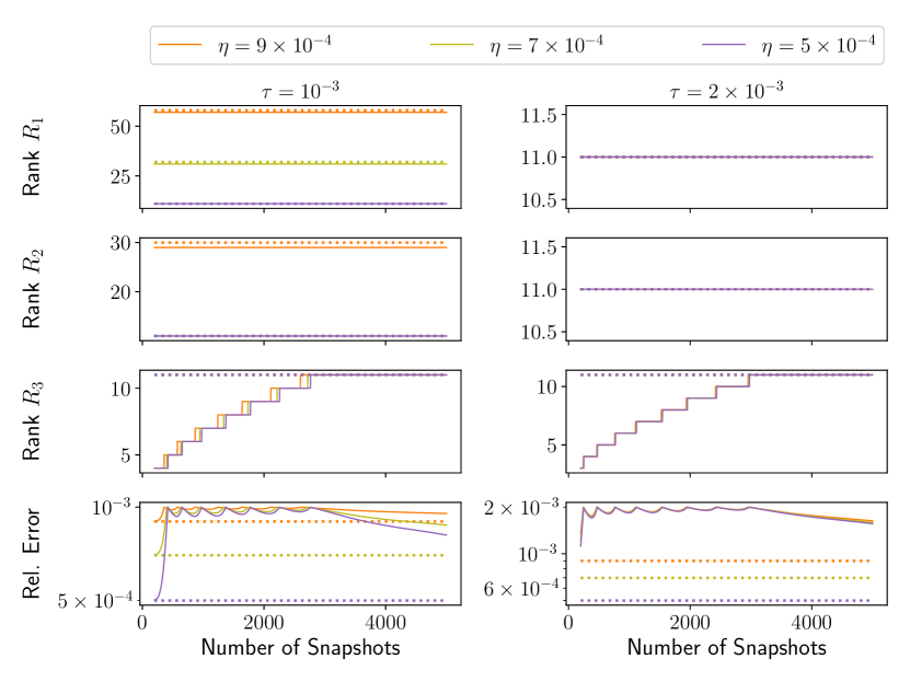
Figure 3: Growth of Tucker ranks $R_{1},R_{2},R_{3}$ and relative error in the Tucker approximation of data tensors, as we insert slices one by one with our streaming algorithm, after initial ST-HOSVD with 200 snapshots. We show results from three $100\times 100\times 5000$ “sine wave” datasets with approximate Tucker ranks $(R_{1},R_{2},R_{3})=(11,11,11)$. The results from three noise-to-signal ratios $\eta\in\{9,7,5\}\times 10^{-4}$ are represented by different colors; the dotted lines represent the rank/error corresponding to the batch algorithm. The results from the different ST-HOSVD tolerances $\tau\in\{1,2\}\times 10^{-3}$ are shown in the left and right panels.

Consider the $d$-dimensional tensor $\bar{\bm{\mathscr{{X}}}}\in\mathbb{R}^{N_{1}\times\cdots\times N_{d}}$, constructed from sampling the function

$$f(x_{1},\ldots,x_{d})=\sum_{j_{1}=-J_{1}}^{J_{1}}\cdots\sum_{j_{d}=-J_{d}}^{J_{d}}c_{j_{1},\ldots,j_{d}}\sin(j_{1}x_{1}+\cdots+j_{d}x_{d})$$ (39)

on a uniform grid in the domain $[0,2\pi]^{d}$. Using trigonometric “sum of angles” identities, we can easily establish that the exact rank of the $k$-th unfolding $\bar{{\bm{\mathbf{{X}}}}}_{(k)}$ is $R_{k}=2J_{k}+1$, and the $d$-dimensional Tucker core $\bar{\bm{\mathscr{{C}}}}$ of this tensor has dimensions $R_{1}\times\cdots\times R_{d}$. In our experiments, we add noise to construct our data tensor as

$$\bm{\mathscr{{X}}}=\bar{\bm{\mathscr{{X}}}}+\bm{\mathscr{{N}}},$$ (40)

where the entries of the additive noise tensor are drawn from the standard Gaussian distribution and scaled such that

$$\lVert\bm{\mathscr{{N}}}(:,\ldots,:,i_{d})\rVert_{F}=\eta\lVert\bm{\mathscr{{X}}}(:,\ldots,:,i_{d})\rVert_{F},\quad 1\leq i_{d}\leq N_{d},$$ (41)

for some chosen noise-to-signal ratio $0\leq\eta<1$. We compress these “sine wave” data tensors using batch ST-HOSVD and streaming ST-HOSVD with various error tolerances $\tau>\eta$.

In fig. 3, we plot the variation of the Tucker ranks and the reconstruction error as we construct the streaming approximation of $100\times 100\times 5000$ data tensors, with approximate ranks $11\times 11\times 11$ and different noise-to-signal ratios $\eta\in\{9,7,5\}\times 10^{-4}$, using the streaming ST-HOSVD algorithm with two relative tolerances $\tau\in\{1,2\}\times 10^{-3}$. We note that when the noise level and the relative tolerance is well separated, our algorithm can recover the underlying low-rank structure accurately; however, when the separation is small (e.g. $\tau=10^{-3}$ and $\eta=9\times 10^{-4}$), the estimated ranks are higher than the true ranks.

Table 1: Comparison of batch and streaming ST-HOSVD methods, when compressing synthetic “sine wave” data tensors with mode sizes $(N_{1},N_{2},N_{3})=(100,100,5000)$ and approximate Tucker ranks $(R_{1},R_{2},R_{3})=(11,11,11)$, with various noise-to-signal ratios and ST-HOSVD tolerances (streaming compressions are initialized with 200 snapshots). We report the Tucker ranks, maximum ST-HOSVD memeory usage (in MBs), and computation time (in seconds).

Noise	Tolerance	Batch ST-HOSVD			Streaming ST-HOSVD
($\eta$)	($\tau$)	Rank	Memory	Time	Rank	Memory	Time
$9\times 10^{-4}$	$1\times 10^{-3}$	$(59,31,11)$	709.40	5.13	$(57,29,11)$	27.84	3.29
	$2\times 10^{-3}$	$(11,11,11)$	605.54	5.58	$(11,11,11)$	17.98	2.02
$7\times 10^{-4}$	$1\times 10^{-3}$	$(32,11,11)$	614.80	6.24	$(31,11,11)$	21.54	2.31
	$2\times 10^{-3}$	$(11,11,11)$	605.54	6.15	$(11,11,11)$	17.98	2.06
$5\times 10^{-4}$	$1\times 10^{-3}$	$(11,11,11)$	605.54	5.95	$(11,11,11)$	17.98	2.34
	$2\times 10^{-3}$	$(11,11,11)$	605.54	5.51	$(11,11,11)$	17.98	2.11

We also compare the final performance of the streaming algorithm against the standard batch ST-HOSVD in table 1; the results indicate both the streaming and batch versions recover comparable Tucker ranks from the datasets. However, we see an advantage in terms of the memory usage and computational time. During the incremental updates, our algorithm uses far less memory compared to the batch version. Moreover, the cubic computational cost of the required eigendecomposition along the streaming mode is replaced by constant computational cost per slice insertion (assuming the rank does not increase drastically). This reduces the overall computational time when the streaming mode size is larger than the non-streaming mode sizes.

5.2 HCCI combustion dataset

(a) Original dataset

(b) Reconstructed dataset, $\tau=10^{-1}$

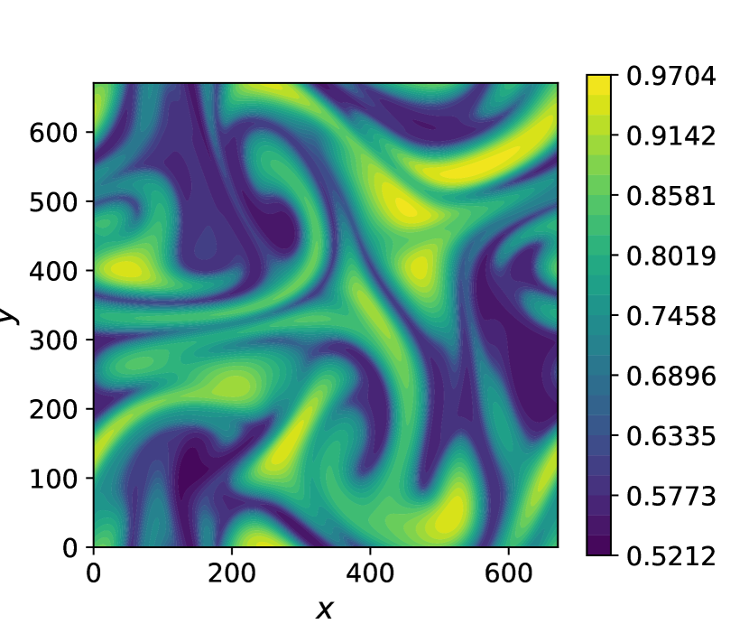
(c) Reconstructed dataset, $\tau=10^{-2}$

(d) Reconstructed dataset, $\tau=10^{-3}$

(e) Reconstruction error, $\tau=10^{-1}$

(f) Reconstruction error, $\tau=10^{-2}$

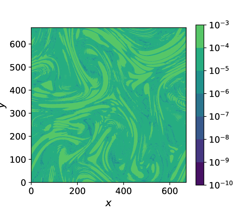
(g) Reconstruction error, $\tau=10^{-3}$

Figure 4: Visual comparison between the original data tensor and reconstructed streaming Tucker tensor at different compression tolerances. We consider the temperature variable across the spatial modes at time $t=2\times 10^{-3}$ s, and reconstruct it from the streaming Tucker compressed tensor initialized with 150 snapshots. The top figure is the original field, the middle row depicts the reconstructed fields for $\tau\in\{10^{-1},10^{-2},10^{-3}\}$, and the bottom row plots the difference between the original and reconstructed fields.

Following a previous study [11], we consider a simulation of auto-ignition processes of a turbulent ethanol-air mixture, under conditions corresponding to a homogeneous charge compression ignition (HCCI) combustion mode of an internal combustion engine, to assess the streaming ST-HOSVD algorithm applied to scientific data. The simulation was performed on a rectangular Cartesian grid of a 2D spatial domain with $672\times 672$ grid points, which constitute the first two modes of the tensor. The simulation state comprises 33 variables at each grid point—the third mode—and 268 time snapshots (the last of a total of 626 timesteps) are considered which constitutes the streaming mode of a fourth-order tensor. Since this is not a synthetic data set with an exact known low-rank structure, the results of the streaming and batch ST-HOSVD algorithms are likely to produce different results due to our lack of knowledge about the exact truncation criteria; however they should still be comparable for a fixed relative error tolerance $\tau$.

In fig. 4, we compare the reconstructions from the streaming Tucker compression (initialized with 150 timesteps of interest) against the original dataset at three tolerance levels: $\tau\in\{10^{-1},10^{-2},10^{-3}\}$. We observe that, as the tolerance is tightened, the contours of the element-wise reconstructions become visually nearly identical to the contours of the original data.

Table 2: Performance of the batch and streaming ST-HOSVD methods, when compressing the HCCI combustion data tensor with mode sizes $(N_{1},N_{2},N_{3},N_{4})=(672,672,33,268)$, at three ST-HOSVD tolerances. Streaming compressions are initialized with 110, 130, and 150 snapshots. We report the Tucker ranks, maximum ST-HOSVD memeory usage (in GBs), computation time (in seconds), and estimated relative reconstruction errors.

Tolerance ($\tau$)	Algorithm	Rank	Memory	Time	Relative Error
$10^{-1}$	Batch	$(35,27,8,7)$	33.68	20.91	$9.6\times 10^{-2}$
	Streaming (110)	$(46,37,9,7)$	14.06	20.59	$9.4\times 10^{-2}$
	Streaming (130)	$(44,36,9,8)$	16.57	19.55	$9.6\times 10^{-2}$
	Streaming (150)	$(43,34,9,9)$	19.09	21.23	$1.0\times 10^{-1}$
$10^{-2}$	Batch	$(122,110,21,29)$	38.70	22.65	$9.6\times 10^{-3}$
	Streaming (110)	$(139,126,24,28)$	16.34	29.24	$9.6\times 10^{-3}$
	Streaming (130)	$(137,124,23,27)$	19.24	28.93	$9.9\times 10^{-3}$
	Streaming (150)	$(134,121,23,28)$	22.09	28.15	$9.6\times 10^{-3}$
$10^{-3}$	Batch	$(231,213,29,67)$	46.42	24.43	$9.5\times 10^{-4}$
	Streaming (110)	$(249,230,30,96)$	19.64	65.65	$9.8\times 10^{-4}$
	Streaming (130)	$(248,227,30,77)$	23.15	56.51	$9.9\times 10^{-4}$
	Streaming (150)	$(245,225,30,64)$	26.59	50.90	$9.8\times 10^{-4}$

In table 2, we compare the performance of the batch and streaming Tucker factorizations. We compress the data tensor with three error tolerances, and initialize the streaming versions with data from the first 110, 130, and 150 timesteps of interest. We observe that the target error tolerance is satisfied in all the experiments. Additionally, as we increase the number of initial time steps, the Tucker ranks from the streaming algorithm approach those computed from the batch algorithm, while simultaneously lowering the total computational time for the factorization. This improvement, however, comes at the cost of increasing memory footprint of the streaming algorithm (which is still smaller compared to the batch version).

6 Conclusions and future work

In this paper, we introduced an algorithm for constructing Tucker factorizations of streaming data; we start from an initial ST-HOSVD factorization and update it as new tensor slices are incorporated one at a time while ensuring the relative reconstruction error stays within a specified fixed tolerance. In our experiments, we observed that the streaming version may on occasion overestimate the Tucker ranks when compared to the batch algorithm, but the former generally has a smaller memory footprint. Additionally, this rank-overestimation can be controlled by supplying a larger number of snapshots to the initial ST-HOSVD. Finally, when the size of the streaming mode is large compared to the product of Tucker ranks along the non-streaming modes, the streaming version usually outperforms the batch algorithm in terms of computational time. In summary, our algorithm is particularly suited to approximately low-rank ($R_{k}\ll N_{k}$) tensors with large streaming mode size ($N_{d}\gg R_{1}\cdots R_{d-1}$).

We note that our algorithm uses, for the most part, the computational kernels already implemented in TuckerMPI (e.g. TTM, Gram-SVD). These kernels have already been significantly optimized for distributed implementation by Ballard et al. [2], and we can leverage those implementations. The only additional kernels are zero-paddings (lines 13 and 14 of algorithm 2), tensor concatenation (line 15), and the incremental SVD update step (line 19). The first two operations result in an increased size of the core tensor and a projection approximation of the new tensor slice; a parallel implementation essentially boils down to keeping track of tensor partitions across multiple MPI ranks, and re-partitioning appropriately. The incremental SVD update along the streaming mode can be accomplished using a Gram-SVD which has been shown to be scalable [1]. In future, we want to implement this fully distributed streaming ST-HOSVD update algorithm, which will allow compression of extreme-scale scientific datasets.

Additionally, we wish to adapt our algorithm to inserting multiple data slices at once, and utilize the advanced incremental SVD algorithms developed in [3, 5]; this will likely reduce dependency on the size of initial batch factorization, stabilize the rank growth, and lead to better approximations of data tensors.

Ackowledgements

This work was performed as part of the ExaLearn Co-design Center, supported by the Exascale Computing Project (17-SC-20-SC), a collaborative effort of the U.S. Department of Energy Office of Science and the National Nuclear Security Administration. Sandia National Laboratories is a multi-mission laboratory managed and operated by National Technology and Engineering Solutions of Sandia, LLC.,a wholly owned subsidiary of Honeywell International, Inc., for the U.S. Department of Energy’s National Nuclear Security Administration under contract DE-NA-0003525. The views expressed in the article do not necessarily represent the views of the U.S. Department of Energy or the United States Government.

Appendix A Derivation of incremental SVD error bound

In constructing best $r$-rank approximation of ${\bm{\mathbf{{A}}}}\in\mathbb{R}^{m\times n}$ using SVD:

$${\bm{\mathbf{{A}}}}={\bm{\mathbf{{U}}}}{\bm{\mathbf{{S}}}}{\bm{\mathbf{{V}}}}+{\bm{\mathbf{{E}}}},$$

we are guaranteed that:

• ${\bm{\mathbf{{U}}}}$ has orthonormal columns: ${\bm{\mathbf{{U}}}}^{\top}{\bm{\mathbf{{U}}}}={\bm{\mathbf{{I}}}}_{r}$, and

• Columns of error ${\bm{\mathbf{{E}}}}$ are orthogonal to the column span of ${\bm{\mathbf{{U}}}}$: ${\bm{\mathbf{{U}}}}^{\top}{\bm{\mathbf{{E}}}}={\bm{\mathbf{{0}}}}_{r\times n}$.

Let ${\bm{\mathbf{{W}}}}\in\mathbb{R}^{m\times(m-r)}$ be such that the columns of ${\bm{\mathbf{{U}}}}$ and ${\bm{\mathbf{{W}}}}$ together form a orthonormal basis of $\mathbb{R}^{m}$; then

• ${\bm{\mathbf{{W}}}}^{\top}{\bm{\mathbf{{U}}}}={\bm{\mathbf{{0}}}}_{(m-r)\times r}$, and

• $\textrm{span}({\bm{\mathbf{{E}}}})\subseteq\textrm{span}({\bm{\mathbf{{W}}}})$.

Next, in the approximate SVD of the “internal” matrix:

$$\begin{bmatrix}{\bm{\mathbf{{S}}}}&\\ {\bm{\mathbf{{P}}}}&{\bm{\mathbf{{L}}}}\end{bmatrix}={\bm{\mathbf{{U}}}}^{\prime}\tilde{{\bm{\mathbf{{S}}}}}{\bm{\mathbf{{V}}}}^{\prime}+{\bm{\mathbf{{E}}}}^{\prime}\in\mathbb{R}^{(r+p)\times(r+s)},$$

partition the error into rectangular blocks:

$${\bm{\mathbf{{E}}}}^{\prime}=\begin{bmatrix}{\bm{\mathbf{{E}}}}^{\prime}_{11}&{\bm{\mathbf{{E}}}}^{\prime}_{12}\\ {\bm{\mathbf{{E}}}}^{\prime}_{21}&{\bm{\mathbf{{E}}}}^{\prime}_{22}\end{bmatrix},\quad{\bm{\mathbf{{E}}}}^{\prime}_{11}\in\mathbb{R}^{r\times r},\quad{\bm{\mathbf{{E}}}}^{\prime}_{22}\in\mathbb{R}^{p\times s}.$$

Using these notations, we start simplifying the final error of the incremental SVD; we have:

$$\tilde{{\bm{\mathbf{{A}}}}}-\tilde{{\bm{\mathbf{{U}}}}}\tilde{{\bm{\mathbf{{S}}}}}\tilde{{\bm{\mathbf{{V}}}}}=\begin{bmatrix}{\bm{\mathbf{{A}}}}\\ {\bm{\mathbf{{B}}}}\end{bmatrix}-\begin{bmatrix}{\bm{\mathbf{{U}}}}&\\ &{\bm{\mathbf{{I}}}}_{p}\end{bmatrix}{\bm{\mathbf{{U}}}}^{\prime}\tilde{{\bm{\mathbf{{S}}}}}{\bm{\mathbf{{V}}}}^{\prime}\begin{bmatrix}{\bm{\mathbf{{V}}}}\\ {\bm{\mathbf{{Q}}}}\end{bmatrix}.$$

Since ${\bm{\mathbf{{A}}}}={\bm{\mathbf{{U}}}}{\bm{\mathbf{{S}}}}{\bm{\mathbf{{V}}}}+{\bm{\mathbf{{E}}}}$ and ${\bm{\mathbf{{B}}}}={\bm{\mathbf{{P}}}}{\bm{\mathbf{{V}}}}+{\bm{\mathbf{{L}}}}{\bm{\mathbf{{Q}}}}$, we can simplify:

$$\tilde{{\bm{\mathbf{{A}}}}}-\tilde{{\bm{\mathbf{{U}}}}}\tilde{{\bm{\mathbf{{S}}}}}\tilde{{\bm{\mathbf{{V}}}}}=\begin{bmatrix}{\bm{\mathbf{{E}}}}\\ \hbox{}\end{bmatrix}+\begin{bmatrix}{\bm{\mathbf{{U}}}}{\bm{\mathbf{{S}}}}{\bm{\mathbf{{V}}}}\\ {\bm{\mathbf{{P}}}}{\bm{\mathbf{{V}}}}+{\bm{\mathbf{{L}}}}{\bm{\mathbf{{Q}}}}\end{bmatrix}-\begin{bmatrix}{\bm{\mathbf{{U}}}}&\\ &{\bm{\mathbf{{I}}}}_{p}\end{bmatrix}{\bm{\mathbf{{U}}}}^{\prime}\tilde{{\bm{\mathbf{{S}}}}}{\bm{\mathbf{{V}}}}^{\prime}\begin{bmatrix}{\bm{\mathbf{{V}}}}\\ {\bm{\mathbf{{Q}}}}\end{bmatrix}.$$

Using the factorization in eq. 36, we obtain:

$$\tilde{{\bm{\mathbf{{A}}}}}-\tilde{{\bm{\mathbf{{U}}}}}\tilde{{\bm{\mathbf{{S}}}}}\tilde{{\bm{\mathbf{{V}}}}} =\begin{bmatrix}{\bm{\mathbf{{E}}}}\\ \hbox{}\end{bmatrix}+\begin{bmatrix}{\bm{\mathbf{{U}}}}&\\ &{\bm{\mathbf{{I}}}}_{p}\end{bmatrix}{\bm{\mathbf{{S}}}}^{\prime}\begin{bmatrix}{\bm{\mathbf{{V}}}}\\ {\bm{\mathbf{{Q}}}}\end{bmatrix}-\begin{bmatrix}{\bm{\mathbf{{U}}}}&\\ &{\bm{\mathbf{{I}}}}_{p}\end{bmatrix}{\bm{\mathbf{{U}}}}^{\prime}\tilde{{\bm{\mathbf{{S}}}}}{\bm{\mathbf{{V}}}}^{\prime}\begin{bmatrix}{\bm{\mathbf{{V}}}}\\ {\bm{\mathbf{{Q}}}}\end{bmatrix}$$

$$=\begin{bmatrix}{\bm{\mathbf{{E}}}}\\ \hbox{}\end{bmatrix}+\begin{bmatrix}{\bm{\mathbf{{U}}}}&\\ &{\bm{\mathbf{{I}}}}_{p}\end{bmatrix}({\bm{\mathbf{{S}}}}^{\prime}-{\bm{\mathbf{{U}}}}^{\prime}\tilde{{\bm{\mathbf{{S}}}}}{\bm{\mathbf{{V}}}}^{\prime})\begin{bmatrix}{\bm{\mathbf{{V}}}}\\ {\bm{\mathbf{{Q}}}}\end{bmatrix}$$

$$=\begin{bmatrix}{\bm{\mathbf{{E}}}}\\ \hbox{}\end{bmatrix}+\begin{bmatrix}{\bm{\mathbf{{U}}}}&\\ &{\bm{\mathbf{{I}}}}_{p}\end{bmatrix}{\bm{\mathbf{{E}}}}^{\prime}\begin{bmatrix}{\bm{\mathbf{{V}}}}\\ {\bm{\mathbf{{Q}}}}\end{bmatrix}$$

$$=\begin{bmatrix}{\bm{\mathbf{{E}}}}\\ \hbox{}\end{bmatrix}+\begin{bmatrix}{\bm{\mathbf{{U}}}}&\\ &{\bm{\mathbf{{I}}}}_{p}\end{bmatrix}\begin{bmatrix}{\bm{\mathbf{{E}}}}^{\prime}_{11}&{\bm{\mathbf{{E}}}}^{\prime}_{12}\\ {\bm{\mathbf{{E}}}}^{\prime}_{21}&{\bm{\mathbf{{E}}}}^{\prime}_{22}\end{bmatrix}\begin{bmatrix}{\bm{\mathbf{{V}}}}\\ {\bm{\mathbf{{Q}}}}\end{bmatrix}$$

$$=\begin{bmatrix}{\bm{\mathbf{{E}}}}\\ \hbox{}\end{bmatrix}+\begin{bmatrix}{\bm{\mathbf{{U}}}}&\\ &{\bm{\mathbf{{I}}}}_{p}\end{bmatrix}\begin{bmatrix}{\bm{\mathbf{{E}}}}^{\prime}_{11}{\bm{\mathbf{{V}}}}+{\bm{\mathbf{{E}}}}^{\prime}_{12}{\bm{\mathbf{{Q}}}}\\ {\bm{\mathbf{{E}}}}^{\prime}_{21}{\bm{\mathbf{{V}}}}+{\bm{\mathbf{{E}}}}^{\prime}_{22}{\bm{\mathbf{{Q}}}}\end{bmatrix}.$$

Multiplying this entire expression on the left by an orthogonal matrix (which won’t change the Frobenius norm), we obtain

$$\begin{bmatrix}{\bm{\mathbf{{U}}}}^{\top}&\\ {\bm{\mathbf{{W}}}}^{\top}&\\ &{\bm{\mathbf{{I}}}}_{p}\end{bmatrix}(\tilde{{\bm{\mathbf{{A}}}}}-\tilde{{\bm{\mathbf{{U}}}}}\tilde{{\bm{\mathbf{{S}}}}}\tilde{{\bm{\mathbf{{V}}}}}) =\begin{bmatrix}{\bm{\mathbf{{U}}}}^{\top}{\bm{\mathbf{{E}}}}\\ {\bm{\mathbf{{W}}}}^{\top}{\bm{\mathbf{{E}}}}\\ \hbox{}\end{bmatrix}+\begin{bmatrix}{\bm{\mathbf{{U}}}}^{\top}{\bm{\mathbf{{U}}}}&\\ {\bm{\mathbf{{W}}}}^{\top}{\bm{\mathbf{{U}}}}&\\ &{\bm{\mathbf{{I}}}}_{p}\end{bmatrix}\begin{bmatrix}{\bm{\mathbf{{E}}}}^{\prime}_{11}{\bm{\mathbf{{V}}}}+{\bm{\mathbf{{E}}}}^{\prime}_{12}{\bm{\mathbf{{Q}}}}\\ {\bm{\mathbf{{E}}}}^{\prime}_{21}{\bm{\mathbf{{V}}}}+{\bm{\mathbf{{E}}}}^{\prime}_{22}{\bm{\mathbf{{Q}}}}\end{bmatrix}$$

$$=\begin{bmatrix}\hbox{}\\ {\bm{\mathbf{{W}}}}^{\top}{\bm{\mathbf{{E}}}}\\ \hbox{}\end{bmatrix}+\begin{bmatrix}{\bm{\mathbf{{I}}}}_{r}&\\ \hbox{}&\\ &{\bm{\mathbf{{I}}}}_{p}\end{bmatrix}\begin{bmatrix}{\bm{\mathbf{{E}}}}^{\prime}_{11}{\bm{\mathbf{{V}}}}+{\bm{\mathbf{{E}}}}^{\prime}_{12}{\bm{\mathbf{{Q}}}}\\ {\bm{\mathbf{{E}}}}^{\prime}_{21}{\bm{\mathbf{{V}}}}+{\bm{\mathbf{{E}}}}^{\prime}_{22}{\bm{\mathbf{{Q}}}}\end{bmatrix}$$

$$=\begin{bmatrix}\hbox{}\\ {\bm{\mathbf{{W}}}}^{\top}{\bm{\mathbf{{E}}}}\\ \hbox{}\end{bmatrix}+\begin{bmatrix}{\bm{\mathbf{{E}}}}^{\prime}_{11}{\bm{\mathbf{{V}}}}+{\bm{\mathbf{{E}}}}^{\prime}_{12}{\bm{\mathbf{{Q}}}}\\ \hbox{}\\ {\bm{\mathbf{{E}}}}^{\prime}_{21}{\bm{\mathbf{{V}}}}+{\bm{\mathbf{{E}}}}^{\prime}_{22}{\bm{\mathbf{{Q}}}}\end{bmatrix}$$

$$=\begin{bmatrix}{\bm{\mathbf{{E}}}}^{\prime}_{11}{\bm{\mathbf{{V}}}}+{\bm{\mathbf{{E}}}}^{\prime}_{12}{\bm{\mathbf{{Q}}}}\\ {\bm{\mathbf{{W}}}}^{\top}{\bm{\mathbf{{E}}}}\\ {\bm{\mathbf{{E}}}}^{\prime}_{21}{\bm{\mathbf{{V}}}}+{\bm{\mathbf{{E}}}}^{\prime}_{22}{\bm{\mathbf{{Q}}}}\end{bmatrix},$$

and consequently:

$$\lVert\tilde{{\bm{\mathbf{{A}}}}}-\tilde{{\bm{\mathbf{{U}}}}}\tilde{{\bm{\mathbf{{S}}}}}\tilde{{\bm{\mathbf{{V}}}}}\rVert_{F}^{2}=\lVert{\bm{\mathbf{{E}}}}^{\prime}_{11}{\bm{\mathbf{{V}}}}+{\bm{\mathbf{{E}}}}^{\prime}_{12}{\bm{\mathbf{{Q}}}}\rVert_{F}^{2}+\lVert{\bm{\mathbf{{W}}}}^{\top}{\bm{\mathbf{{E}}}}\rVert_{F}^{2}+\lVert{\bm{\mathbf{{E}}}}^{\prime}_{21}{\bm{\mathbf{{V}}}}+{\bm{\mathbf{{E}}}}^{\prime}_{22}{\bm{\mathbf{{Q}}}}\rVert_{F}^{2}.$$

Now, left multiplication by matrix with orthonormal columns, or right multiplication by matrix with orthonormal rows does not change Frobenius norm. Since $W$ has orthonormal columns, we obtain:

$$\lVert{\bm{\mathbf{{W}}}}^{\top}{\bm{\mathbf{{E}}}}\rVert_{F}=\lVert{\bm{\mathbf{{W}}}}{\bm{\mathbf{{W}}}}^{\top}{\bm{\mathbf{{E}}}}\rVert_{F}=\lVert{\bm{\mathbf{{E}}}}\rVert_{F},$$

where the last equality follows because $\textrm{span}({\bm{\mathbf{{E}}}})\subseteq\textrm{span}({\bm{\mathbf{{W}}}})$, therefore the projection ${\bm{\mathbf{{W}}}}{\bm{\mathbf{{W}}}}^{\top}$ leaves ${\bm{\mathbf{{E}}}}$ unchanged: ${\bm{\mathbf{{W}}}}{\bm{\mathbf{{W}}}}^{\top}{\bm{\mathbf{{E}}}}={\bm{\mathbf{{E}}}}$. Next, since ${\bm{\mathbf{{V}}}}$ and ${\bm{\mathbf{{Q}}}}$ has orthonormal rows and their row spans are orthogonal, we obtain:

$$\begin{split}\lVert{\bm{\mathbf{{E}}}}^{\prime}_{11}{\bm{\mathbf{{V}}}}+{\bm{\mathbf{{E}}}}^{\prime}_{12}{\bm{\mathbf{{Q}}}}\rVert_{F}^{2}=\left\lVert\begin{bmatrix}{\bm{\mathbf{{E}}}}^{\prime}_{11}&{\bm{\mathbf{{E}}}}^{\prime}_{12}\end{bmatrix}\begin{bmatrix}{\bm{\mathbf{{V}}}}\\ {\bm{\mathbf{{Q}}}}\end{bmatrix}\right\rVert_{F}^{2}&=\left\lVert\begin{bmatrix}{\bm{\mathbf{{E}}}}^{\prime}_{11}&{\bm{\mathbf{{E}}}}^{\prime}_{12}\end{bmatrix}\right\rVert_{F}^{2}\\ &=\lVert{\bm{\mathbf{{E}}}}^{\prime}_{11}\rVert_{F}^{2}+\lVert{\bm{\mathbf{{E}}}}^{\prime}_{12}\rVert_{F}^{2},\end{split}$$

and similarly $\lVert{\bm{\mathbf{{E}}}}^{\prime}_{21}{\bm{\mathbf{{V}}}}+{\bm{\mathbf{{E}}}}^{\prime}_{22}{\bm{\mathbf{{Q}}}}\rVert_{F}^{2}=\lVert{\bm{\mathbf{{E}}}}^{\prime}_{21}\rVert_{F}^{2}+\lVert{\bm{\mathbf{{E}}}}^{\prime}_{22}\rVert_{F}^{2}$. We finally obtain:

$$\begin{split}\lVert\tilde{{\bm{\mathbf{{A}}}}}-\tilde{{\bm{\mathbf{{U}}}}}\tilde{{\bm{\mathbf{{S}}}}}\tilde{{\bm{\mathbf{{V}}}}}\rVert_{F}^{2}&=\lVert{\bm{\mathbf{{E}}}}^{\prime}_{11}\rVert_{F}^{2}+\lVert{\bm{\mathbf{{E}}}}^{\prime}_{12}\rVert_{F}^{2}+\lVert{\bm{\mathbf{{E}}}}\rVert_{F}^{2}+\lVert{\bm{\mathbf{{E}}}}^{\prime}_{21}\rVert_{F}^{2}+\lVert{\bm{\mathbf{{E}}}}^{\prime}_{22}\rVert_{F}^{2}\\ &=\lVert{\bm{\mathbf{{E}}}}\rVert_{F}^{2}+\lVert{\bm{\mathbf{{E}}}}^{\prime}\rVert_{F}^{2}.\end{split}$$

References

• [1] Woody Austin, Grey Ballard, and Tamara G. Kolda. Parallel tensor compression for large-scale scientific data. In 2016 IEEE International Parallel and Distributed Processing Symposium (IPDPS), pages 912–922, Chicago, USA, 2016. IEEE.
• [2] Grey Ballard, Alicia Klinvex, and Tamara G. Kolda. Tuckermpi: A parallel c++/mpi software package for large-scale data compression via the tucker tensor decomposition. ACM Trans. Math. Softw., 46(2), jun 2020.
• [3] Matthew Brand. Incremental singular value decomposition of uncertain data with missing values. In Anders Heyden, Gunnar Sparr, Mads Nielsen, and Peter Johansen, editors, Computer Vision — ECCV 2002, pages 707–720, Berlin, Heidelberg, 2002. Springer Berlin Heidelberg.
• [4] Matthew Brand. Fast low-rank modifications of the thin singular value decomposition. Linear Algebra and its Applications, 415(1):20–30, 2006. Special Issue on Large Scale Linear and Nonlinear Eigenvalue Problems.
• [5] Yongsheng Cheng, Jiang Zhu, and Xiaokang Lin. An enhanced incremental SVD algorithm for change point detection in dynamic networks. IEEE Access, 6, 2018.
• [6] Lieven De Lathauwer, Bart De Moor, and Joos Vandewalle. A multilinear singular value decomposition. SIAM Journal on Matrix Analysis and Applications, 21(4):1253–1278, 2000.
• [7] Ekta Gujral, Ravdeep Pasricha, and Evangelos E. Papalexakis. SamBaTen: Sampling-based batch incremental tensor decomposition. In Proceedings of the 2018 SIAM International Conference on Data Mining, pages 387–395, San Diego, USA, 2018. SIAM.
• [8] Weiming Hu, Xi Li, Xiaoqin Zhang, Xinchu Shi, Stephen Maybank, and Zhongfei Zhang. Incremental tensor subspace learning and its applications to foreground segmentation and tracking. International Journal of Computer Vision, 91(3):303–327, 2011.
• [9] Jun-Gi Jang and U. Kang. Static and streaming tucker decomposition for dense tensors. ACM Transactions on Knowledge Discovery from Data, 17:1–34, 2023.
• [10] Hiroyuki Kasai. Online low-rank tensor subspace tracking from incomplete data by CP decomposition using recursive least squares. In 2016 IEEE International Conference on Acoustics, Speech and Signal Processing (ICASSP), Shanghai, China, March 2016. IEEE.
• [11] Hemanth Kolla, Konduri Aditya, and Jacqueline H. Chen. Higher Order Tensors for DNS Data Analysis and Compression, pages 109–134. Springer International Publishing, Cham, 2020.
• [12] Pierre-David Letourneau, Muthu Baskaran, Tom Henretty, James Ezick, and Richard Lethin. Computationally efficient CP tensor decomposition update framework for emerging component discovery in streaming data. In HPEC’18 Proceedings, Boston, USA, 2018. IEEE.
• [13] X. Ma, D. Schonfeld, and A. Khokhar. Dynamic updating and downdating matrix SVD and tensor HOSVD for adaptive indexing and retrieval of motion trajectories. In 2009 IEEE International Conference on Acoustics, Speech and Signal Processing, pages 1129–1132, Taipei, Taiwan, 2009. IEEE.
• [14] Osman Asif Malik and Stephen Becker. Low-rank tucker decomposition of large tensors using TensorSketch. In Advances in Neural Information Processing Systems, pages 10116–10126, Montréal, Canada, 2018. Curran Associates, Inc.
• [15] Morteza Mardani, Gonzalo Mateos, and Georgios B. Giannakis. Subspace learning and imputation for streaming big data matrices and tensors. IEEE Transactions on Signal Processing, 63(10):2663–2677, may 2015.
• [16] D. Nion and N. D. Sidiropoulos. Adaptive algorithms to track the PARAFAC decomposition of a third-order tensor. IEEE Transactions on Signal Processing, 57(6):2299–2310, June 2009.
• [17] Ravdeep Pasricha, Ekta Gujral, and Evangelos E. Papalexakis. Identifying and alleviating concept drift in streaming tensor decomposition. In Machine Learning and Knowledge Discovery in Databases, pages 327–343, Dublin, Ireland, 2019. Springer International Publishing.
• [18] Anh Huy Phan and Andrzej Cichocki. PARAFAC algorithms for large-scale problems. Neurocomputing, 74(11):1970–1984, May 2011.
• [19] David A. Ross, Jongwoo Lim, Ruei-Sung Lin, and Ming-Hsuan Yang. Incremental learning for robust visual tracking. International Journal of Computer Vision, 77(1):125–141, 2008.
• [20] Lei Shi, Aryya Gangopadhyay, and Vandana P. Janeja. Stensr: Spatio-temporal tensor streams for anomaly detection and pattern discovery. Knowledge and Information Systems, 43(2):333–353, 2015.
• [21] Shaden Smith, Kejun Huang, Nicholas D. Sidiropoulos, and George Karypis. Streaming tensor factorization for infinite data sources. In Proceedings of the 2018 SIAM International Conference on Data Mining, pages 81–89, San Diego, USA, 2018. SIAM.
• [22] Andrews Sobral, Christopher G. Baker, Thierry Bouwmans, and El-hadi Zahzah. Incremental and multi-feature tensor subspace learning applied for background modeling and subtraction. In Aurélio Campilho and Mohamed Kamel, editors, Image Analysis and Recognition, pages 94–103, Cham, 2014. Springer International Publishing.
• [23] Qingquan Song, Xiao Huang, Hancheng Ge, James Caverlee, and Xia Hu. Multi-aspect streaming tensor completion. In Proceedings of the 23rd ACM SIGKDD International Conference on Knowledge Discovery and Data Mining, Halifax, Canada, August 2017. ACM.
• [24] Jimeng Sun, Dacheng Tao, Spiros Papadimitriou, Philip S. Yu, and Christos Faloutsos. Incremental tensor analysis: Theory and applications. ACM Trans. Knowl. Discov. Data, 2(3), October 2008.
• [25] Yiming Sun, Yang Guo, Charlene Luo, Joel Tropp, and Madeleine Udell. Low-rank tucker approximation of a tensor from streaming data. SIAM Journal on Mathematics of Data Science, 2(4):1123–1150, 2020.
• [26] Ledyard R. Tucker. Some mathematical notes on three-mode factor analysis. Psychometrika, 31:279–311, 1966.
• [27] Michiel Vandecappelle, Nico Vervliet, and Lieven De Lathauwer. Nonlinear least squares updating of the canonical polyadic decomposition. In 2017 25th European Signal Processing Conference (EUSIPCO), pages 663–667, Kos island, Greece, aug 2017. IEEE.
• [28] Nick Vannieuwenhoven, Raf Vandebril, and Karl Meerbergen. A New Truncation Strategy for the Higher-Order Singular Value Decomposition. SIAM J. on Sci. Comp., 34(2):A1027–A1052, 2012.
• [29] H. Xiao, F. Wang, F. Ma, and J. Gao. eOTD: An efficient online Tucker decomposition for higher order tensors. In 2018 IEEE International Conference on Data Mining (ICDM), pages 1326–1331, Singapore, 2018. IEEE.
• [30] Yangwen Zhang. An answer to an open question in the incremental svd, 2022.
• [31] Shuo Zhou, Nguyen Xuan Vinh, James Bailey, Yunzhe Jia, and Ian Davidson. Accelerating online CP decompositions for higher order tensors. In KDD’16: Proceedings of the 22nd ACM SIGKDD International Conference on Knowledge Discovery and Data Mining, San Francisco, USA, 2016. ACM.