A new provably stable weighted state redistribution algorithm

Abstract

We propose a practical finite volume method on cut cells using state redistribution. Our algorithm is provably monotone, total variation diminishing, and GKS stable in many situations, and shuts off smoothly as the cut cell size approaches a target value. Our analysis reveals why original state redistribution works so well: it results in a monotone scheme for most configurations, though at times subject to a slightly smaller CFL condition. Our analysis also explains why a pre-merging step is beneficial. We show computational experiments in two and three dimensions.

65M08, 65M12, 35L02, 35L65

1 Introduction

State redistribution methods were introduced several years ago [2] as a technique to stabilize finite volume updates on cut cells in an otherwise regular Cartesian mesh. It applies a post-processing step to small cut cells by “merging” only temporarily with one or more neighboring cells in a volume weighted fashion and then reconstructing the solution back on to the Cartesian cut cell mesh. The merging and redistribution steps are done in a way that maintains conservation, and is linearity preserving. (The algorithm is presented for a model problem in Section 2 of this paper.) The cut cell volume fraction threshold of one half was demonstrated in two space dimensions to be stable numerically, and a stability proof for a one dimensional model problem with a cut cell at the boundary was presented.

A second paper [6] proposed a generalization of state redistribution (SRD) that removed the abrupt threshold. It proposed a variation of SRD that smoothly shuts off at one half, so that cells that are only slightly below the threshold receive only a little stabilization. A test case of a supersonic vortex flow with an exact solution showed this generalization was less diffusive that the original SRD, and had less than half the error as central merging, and even normal merging showed a 10-15% improvement in error. This paper also extended SRD to three space dimensions, and to the more complicated equations of low Mach number flow with diffusion and compressible flow with combustion.

Cell merging (see [11, 13] for some recent references) is a common alternative for treating small cut cells in an embedded boundary mesh. One advantage of cell merging over SRD is that merged cells can be updated in a monotone way, at least for first order linear advection, and as much as possible for second order schemes using appropriate limiters, time steps and time steppers. An advantage of SRD over cell merging is that it avoids the global merging algorithms that are applied in a preprocessing step. SRD can be applied in a completely local fashion, and it remains stable when two or more cells overlap the same neighboring cell.

This paper develops a systematic framework that addresses both SRD disadvantages above. Motivated by the work in [6] we propose new weights that ensure a monotone update in most situations. The weights can also be chosen to smoothly shut off when the volume fraction of a cut cell reaches a threshold. The analysis in this paper shows how to choose the weights to do this. We analyze the new weighted algorithm and show that it is both total variation diminishing (TVD) and monotonicity preserving on a model problem. (Since the scheme is not linear, and has different coefficients on different cells, it is not sufficient to have positive coefficients for monotonicity preservation, nor does TVD imply it in this situation.) The framework for deriving the new weights can also be used to give the original weights, and also those in [6], giving some insight into when they are not monotone. The analysis also gives some insight into why the original weights work so well. Nevertheless there are reasons one might prefer a monotone scheme, especially since it has negligible additional cost.

The authors are aware only of h-box methods [3], and Domain of Dependence methods [5], which are conservative, monotone, and TVD. Some preliminary work has revealed SRD methods applied to discontinuous Galerkin discretizations may result in energy stable cut cell methods too [15].

In the next section we illustrate the new weighted algorithm in a simple setting with a model problem. This sets the stage for the general weighted algorithm, where the notation can be a bit unwieldy. Section 3 introduces the general formulation and proves it is conservative in one dimension. Section 4 states a number of monotonicity results, with the proofs in the Appendix for the most common cases, and in the Supplementary material for some others, so as not to interrupt the presentation with long stretches of algebra. Computational examples in two and three dimensions are in Section 5. Conclusions and directions for future research are in Section 6.

2 A Simple Model Problem with Weights

To illustrate some of the main ideas we use the simple one dimensional model problem of a regular mesh with cells of size $h$ except for one small cell in the middle with size $\alpha h,\,0\leq\alpha<1/2$. This is illustrated in Fig. 1. We can take $\alpha<1/2$ since larger cut cells with $1/2\leq\alpha<1$ are stable without any post-processing at all.

For the linear advection equation $u_{t}+au_{x}=0$, the first order finite volume update is

(1) $$\widehat{U}_{i}^{n}=U^{n}_{i}-\frac{\Delta t}{h_{i}}\,(f^{n}_{i+1/2}-f^{n}_{i-1/2})=U^{n}_{i}-\frac{a\Delta t}{h_{i}}\,(U^{n}_{i}-U^{n}_{i-1}),$$

where $f_{i+1/2}=aU_{i}$. The numerical update for cell 0 will need to be stabilized.

[width=0.8]images/one_small_right

Figure 1: Model problem with one small cell that merges to the right.

Here we introduce the weighted method in the simplest case by having cell 0 merge to the right with cell 1. Other possibilities are to merge to the left with cell -1, or to use central merging which symmetrically merges with both cells -1 and 1.  In Fig. 1 the notation $\widehat{C}_{j}$ indicates the merging neighborhoods for each cell $j$. A full cell is its own neighborhood, whereas cell 0’s neighborhood, $\widehat{C}_{0}$, includes both cells 0 and 1.

The next step is to define the temporarily merged solution $\widehat{Q}_{j}^{n}$ on each merging neighborhood $\widehat{C}_{j}$. Again, all full cells use their own updated solution $\widehat{Q}_{j}^{n}=\widehat{U}_{j}^{n}$. The solution on $\widehat{C}_{0}$ is a weighted linear combination of $\widehat{U}_{0}^{n}$ and $\widehat{U}_{1}^{n}$. The second index in the weights refers to the cell index of the merging neighborhood being created.

(2) $$\widehat{Q}_{0}^{n} =\frac{w_{0,0}\,h_{0}\,}{\widehat{V}_{0}\,h}\widehat{U}_{0}^{n}+\frac{w_{1,0}\,h_{1}\,}{\widehat{V}_{0}\,h}\widehat{U}_{1}^{n}$$

$$=\frac{w_{0,0}\,\alpha\,}{\widehat{V}_{0}}\widehat{U}_{0}^{n}+\frac{w_{1,0}\,}{\widehat{V}_{0}}\widehat{U}_{1}^{n}$$

Note that the terms in the numerator are volume weighted, and $\widehat{V}_{0}$ is the correspondingly weighted volume in the denominator, after dividing by $h$,

(3) $$\widehat{V}_{0}\,h=w_{0,0}\,h_{0}+w_{1,0}\,h_{1}=(w_{0,0}\,\alpha+w_{1,0})\,h$$

The final update assigns the merged solutions back to the original grid. The first index in the weights refers to the solution being assigned an update from the merging neighborhoods. As you will see, the weights will be related. The weighted updates are:

(4) $$U^{n+1}_{0} =w_{0,0}\widehat{Q}_{0}^{n},$$

$$U^{n+1}_{1} =w_{1,0}\widehat{Q}_{0}^{n}+w_{1,1}\widehat{Q}_{1}^{n}.$$

We want the final solution to be a positive combination of the stabilized neighborhood averages, thus we require $0\leq w_{0,0},w_{1,1},w_{1,0}\leq 1$.

By looking at the conservation requirements the weights can be determined. It is only necessary to look at the two cells treated differently, since all others are conservative due to the base finite volume scheme. Writing the updates at time $n+1$ in terms of time $n$ gives

(5) $$\alpha U_{0}^{n+1}+U_{1}^{n+1} =\alpha\,w_{0,0}\,U_{0}^{n}\;+(w_{1,0}+w_{1,1})\,U_{1}^{n}\;+w_{0,0}\,\lambda\,f_{\sm 1/2}^{n}$$

$$\,-\,(w_{1,0}+w_{1,1})\,\lambda\,f_{3/2}^{n}+(w_{1,0}+w_{1,1}-w_{0,0})\lambda\,f_{1/2}^{n}.$$

For conservation, we must have

(6) $$w_{0,0}=1,$$

$$w_{1,0}+w_{1,1}=1.$$

Then (5) reduces to

$$\alpha U_{0}^{n+1}+U_{1}^{n+1}=\alpha U_{0}^{n}+U_{1}^{n}+f_{3/2}^{n}-f_{\sm 1/2}^{n},$$

showing that this version of SRD is conservative.

Equation (6) still has one free parameter, which we can take to be $w_{1,1}$. By substituting the upwind flux $f(U_{i},U_{i+1})=U_{i}$ into the above formulas and defining $\lambda=\frac{a\Delta t}{h}$, we can write the updates as

(7) $$U_{0}^{n+1} =\frac{\lambda\,}{\widehat{V}_{0}}U_{\sm 1}^{n}+\frac{(\alpha-\lambda w_{1,1})}{\widehat{V}_{0}}\,U_{0}^{n}+\frac{(1-\lambda)(1-w_{1,1})\,}{\widehat{V}_{0}}U_{1}^{n},$$

$$U_{1}^{n+1} =(1-w_{1,1})\frac{\lambda\,}{\widehat{V}_{0}}U_{\sm 1}^{n}+(1-(1-\lambda)w_{1,1})\frac{\alpha}{\widehat{V}_{0}}\,U_{0}^{n}+\frac{(1-\lambda)(1-w_{1,1})}{\widehat{V}_{0}}\,U_{1}^{n}.$$

We see that all multipliers are positive except potentially $(\alpha-\lambda w_{1,1})/\widehat{V}_{0}$. By choosing $0\leq w_{1,1}\leq\alpha$ this is positive too, since we must have $\lambda\leq 1$ for stability.

More generally, if there are more cut cells and only those with $\alpha<0.5$ are merged, then for monotonicity on the unmerged cut cells we will need to reduce the CFL (or alternatively merge all cut cells with volume fraction $\leq$ CFL). Remember that the upwind scheme on regular cells of size $h$ has positive coefficients for $\lambda\leq 1$, since $U_{i}^{n+1}=(1-\lambda)\,U_{i}^{n}+\lambda\,U_{i-1}^{n}$. If cells with volume fraction greater than one half are not merged, for them to be monotone we need to take $\lambda\leq 0.5$. In this case the the coefficient $\alpha-\lambda w_{1,1}$ is positive if $w_{1,1}\leq 2\alpha$. In either case the update concludes by taking $w_{1,0}=1-w_{1,1}$ using (6). Note that the weights shut off smoothly as $\alpha\rightarrow V_{\text{target}}$, where the specified target threshold is either 0.5 or 1.0.

Note that if we instead take $w_{1,1}=0$ and $w_{1,0}=1$, the resulting scheme is another way to describe cell merging. If we start with $U_{0}^{n}=U_{1}^{n}$ then the update formulas (7) are identical and give $U_{0}^{n+1}=U_{1}^{n+1}$ In both cases, the update coefficients are all positive and sum to one, so there will be no new extrema during time-stepping. One can also show this scheme is monotonicity preserving and TVD, but this must be shown directly since it does not follow from positive coefficients on an irregular grid.

For comparison, the original SRD algorithm used $w_{1,1}=w_{1,0}=1/2.$ Equation (7) shows this is not a monotone scheme though we do find it to be well-behaved in practise. For the generalized $\alpha\beta$ SRD scheme in [6], the weights depend on the volume fraction threshold $V_{\text{target}}$ where SRD is activated. For $V_{\text{target}}=1/2$, the corresponding weights are $w_{1,1}=3/4+\alpha/2$ and $w_{1,0}=1/4-\alpha/2$. This is also not monotone but works well in two and three dimensions.

The above example of merging right gives some intuition, but does not always reveal when SRD is monotone. For example, merging to the left results in the following one step update analogous to (7),

(8) $$U_{0}^{n+1} =\frac{\alpha-\lambda}{\widehat{V}_{0}}\,U_{0}^{n}+\frac{\lambda+(1-w_{\sm 1,\sm 1})(1-\lambda)}{\widehat{V}_{0}}\,U_{\sm 1}^{n}+(1-w_{\sm 1,\sm 1})\frac{\lambda}{\widehat{V}_{0}}\,U_{\sm 2}^{n}$$

$$U_{\sm 1}^{n+1} =\frac{(\alpha-\lambda)(1-w_{\sm 1,\sm 1})}{\widehat{V}_{0}}\,U_{0}^{n}+\frac{1-w_{\sm 1,\sm 1}(1-\alpha+\alpha\lambda)}{\widehat{V}_{0}}\,U_{\sm 1}^{n}$$

$$\>+(1-w_{\sm 1,\sm 1}+\alpha w_{\sm 1,\sm 1})\frac{\lambda}{\widehat{V}_{0}}\,U_{\sm 2}^{n}.$$

The unknown weight now is $w_{\sm 1,\sm 1}$ and $\widehat{V}_{0}=\alpha+1-w_{\sm 1,\sm 1}$. It is clear that there is no weight resulting in positive coefficients in front of the $U_{0}^{n}$ terms for the full CFL.

However a small fix to the algorithm does result in a monotone scheme. The first observation is that going from $\widehat{Q}^{n-1}$ to $\widehat{Q}^{n}$ is provably positive. This is stated in more detail in Section 4 and proved in the Appendix. Also, the final assignment from $\widehat{Q}^{n}$ to $U^{n+1}$ is always positive, since it is a convex combination of $Q$’s. If the initial data is stabilized first with an application of SRD (also a convex combination), then the resulting algorithm is provably monotone for merging left up to the full CFL $\lambda=1.$ In other words, given initial conditions $U^{init}$, we apply the SRD algorithm before a finite volume update is performed to get the pre-processed initial condition $U^{0}$

(9) $$U^{0}:=SRD(U^{init}).$$

and then begin time stepping. Pre-merging (as this first step is called) was previously observed to be useful in [6], but we now understand why it is needed. We will exploit this approach in the next sections.

If the original SRD weights of 1/2 are used instead of the new monotone weights for this left-merging neighborhood, and pre-merging is used, it turns out the scheme is monotone for a reduced CFL $\lambda\leq 1/3$. We remark that the original SRD scheme is still stable in the GKS sense for $\lambda\leq 1$ (proved in Appendix B), but it can have some under- or overshoots.

Fig. 2 shows a square wave advecting to the right on a periodic domain [-1,1]. The initial conditions are

(10) $$u(x,0)=\begin{cases}0&x<0\\ 1&x\geq 0\end{cases}$$

so that the jump occurs exactly at the small cell. The one small cell is located exactly in the middle of the domain. There are 20 full cells on each side, so 40 full cells plus the one small cell discretize the domain. The small cell has $\alpha=0.2$. All runs start with a pre-merging step, where the stabilization algorithm is applied to the initial conditions before time stepping begins. The first order upwind scheme is used.

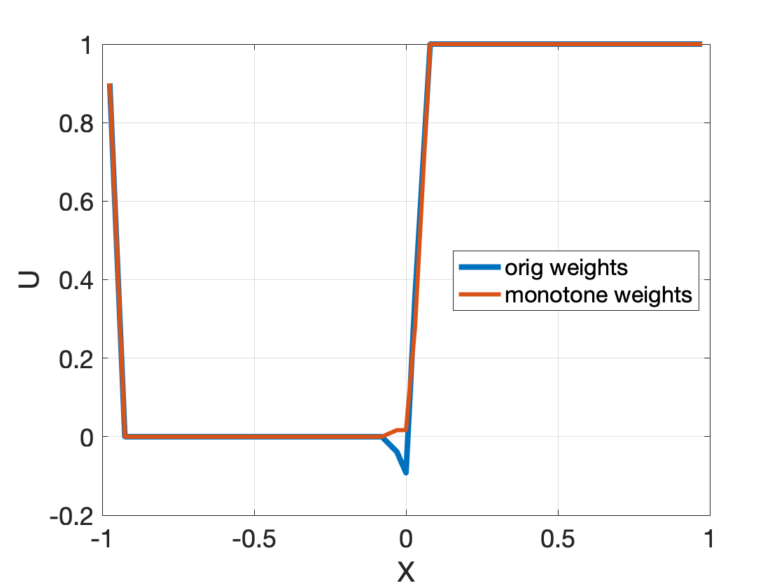
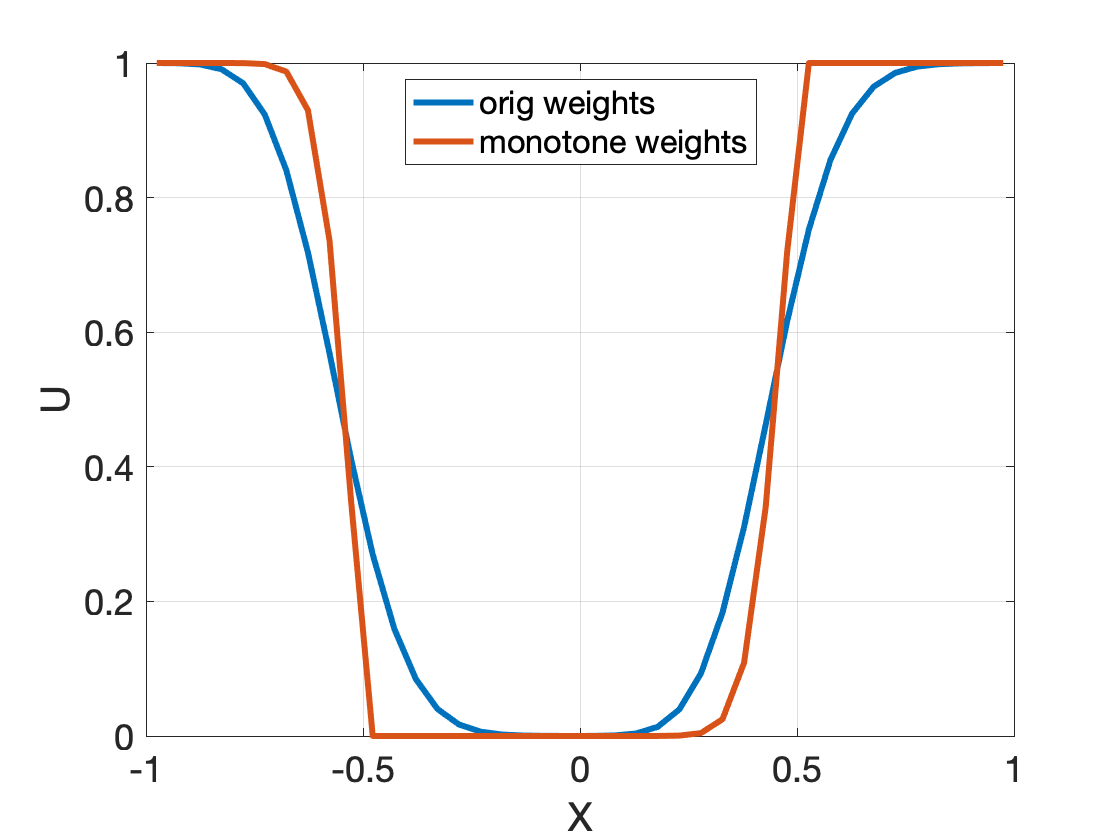
Figure 2: Left figure compares original and new monotone weights after one step using a first-order upwind scheme, with CFL=0.9. The jump is located exactly at the small cell. Right figure compares the monotone weights using the D larger time step with many more steps needed for the original weights at the reduced monotone time step, at time $t=0.448$.

The plot on the left shows two curves after one time step, with a CFL of $\lambda=0.9$, the new monotone weights with $w_{\sm 1,\sm 1}=\alpha$ in blue, and the original weights with $w_{\sm 1,\sm 1}=1/2$ in red. The second plot shows the results at time $t=.448$. The original weights now use a CFL of $\lambda=0.3$ so it is monotone. It takes 30 time steps to reach this time. The new monotone weights still use a CFL of $\lambda=0.9$, and only took 10 steps. The original SRD scheme is much more diffusive with this small time step.

3 Conservation and the Weighted Algorithm in 1D

This section gives some general definitions for the new weighted algorithm and shows a simple proof of conservation. This will include a condition on the weights that we use in Section 4 to show monotonicity. We present this in one space dimension since the notation is already unwieldy with double subscripts.

In the SRD algorithm, recall that $U_{i}^{n}$ is a weighted sum of merging neighborhoods $\widehat{Q}$’s that contribute to cell $i$. We call this set $W_{i}$:

(11) $$U_{i}^{n}=\sum_{j\in W_{i}}\;w_{i,j}\widehat{Q}_{j}^{n-1}.$$

For conservation, we will need

(12) $$\sum_{j\in W_{i}}\;w_{i,j}=1.$$

There is also a set $M_{j}$ of cells that cell $i$ contributes to, defined by

(13) $$\widehat{Q}_{j}^{n-1}=\frac{1}{\widehat{V}_{j}}\sum_{i\in M_{j}}\;w_{i,j}\,h_{i}\,\widehat{U}_{i}^{n-1},$$

where the denominator is the weighted volume $\widehat{V}_{j}=\sum_{i\in M_{j}}\;w_{i,j}\,h_{i}$.

For example in Fig. 1 we have

(14) $$M_{0} =\{0,1\}\hskip 36.135ptW_{0}=\{1\}$$

$$M_{1} =\{1\}\hskip 46.97505ptW_{1}=\{0,1\}.$$

In words, this is because cell 1 is full, so $\widehat{Q}_{1}=\widehat{U}_{1}$, and the cell is its own merging neighborhood. For cell 1, $U_{1}^{n+1}$ is a convex combination of $\widehat{Q}_{0}^{n}$ and $\widehat{Q}_{1}^{n}$, the two cell indices that comprise $W_{1}$. Note that $i\in M_{j}$ is equivalent to $j\in W_{i}$, so only one of the sets needs to be formed when implementing the algorithm.

We start with discrete conservation at time $t^{n}$ and its assignment from the $\widehat{Q}$’s from (11)

(15) $$\sum_{i}V_{i}U^{n}_{i} =\sum_{i}V_{i}\sum_{j\in W_{i}}w_{i,j}\widehat{Q}_{j}^{n-1},$$

where $i$ ranges over all cells in the domain. Rearranging the right-hand-side of the above, and recalling that $j\in W_{i}$ is equivalent to $i\in M_{j}$ we can write

(16) $$\sum_{i}V_{i}U^{n}_{i} =\sum_{i}\sum_{j\in M_{i}}w_{j,i}V_{j}\widehat{Q}_{i}^{n-1}.$$

Recalling the definition of $\widehat{V}_{i}$ this simplifies to

(17) $$\sum_{i}V_{i}U^{n}_{i} =\sum_{i}\widehat{V}_{i}\widehat{Q}_{i}^{n-1}$$

Using the definition of the $\widehat{Q}_{i}$ in (17) we obtain

(18) $$\sum_{i}V_{i}U^{n}_{i} =\sum_{i}\sum_{j\in M_{i}}w_{j,i}V_{j}\widehat{U}_{j}^{n-1}.$$

The above equation (18), has the same form as (16). Thus, it can be re-arranged and becomes

(19) $$\sum_{i}V_{i}U^{n}_{i} =\sum_{i}V_{i}\sum_{j\in W_{i}}w_{i,j}\widehat{U}_{i}^{n-1}.$$

We use the conservation requirement $\sum_{j\in W_{i}}w_{i,j}=1$ from (12), so (19) becomes

(20) $$\sum_{i}V_{i}U^{n}_{i} =\sum_{i}V_{i}\widehat{U}_{i}^{n-1}=\sum_{i}V_{i}U_{i}^{n-1}$$

since the base finite volume scheme is conservative, thus showing that the overall update with SRD is conservative too.

4 Monotonicity for Linear Advection

Based on the intuition and analysis in the previous sections, we have generalized the formulas for the monotone weights to higher dimensions. Here we start by giving the general formula for the weights along with the update formulas from Sec. 3 to have them all in one place:

(21) $$\widehat{Q}_{j}^{n-1} =\frac{1}{\widehat{V}_{j}}\sum_{i\in M_{j}}\;w_{i,j}\,V_{i}\,\widehat{U}_{i}^{n-1}$$

$$\widehat{V}_{j} =\sum_{i\in M_{j}}\;w_{i,j}\,V_{i},$$

$$U_{i}^{n} =\sum_{j\in W_{i}}\;w_{i,j}\widehat{Q}_{j}^{n-1}.$$

where $V_{i}=\alpha_{i}h$ in 1D, and $V_{i}=\alpha_{i}h^{2}$ in 2D. Remembering that $V_{\text{target}}$ is the volume fraction threshold for merging, $N_{i}$ is the number of neighbors that contribute to the final update of cell $i$, and $W_{i}$ the the set of indices of those neighbors, the weights are defined

(22) $$w_{i,j} =\frac{1}{N_{i}-1}(1-\alpha_{j}/V_{\text{target}})\;\text{ for }j\in W_{i}\backslash\{i\}$$

$$w_{i,i} =1-\sum_{j\in W_{i}\backslash\{i\}}w_{i,j}.$$

As with original SRD, the weights can be preprocessed for problems with stationary geometry.

We will prove monotonicity for weighted SRD in several cases of practical interest. These results will always include a pre-merging first step. We derive monotonicity conditions on the weights for merging normal to the boundary for linear advection in 2 space dimensions, with flow parallel to a planar boundary. This is a useful model for the nonlinear Euler equations with wall boundary conditions, and also for incompressible flow or advection of a tracer. Of course we won’t have this exactly in real cases, but as the mesh is refined the boundary approaches linearity, and the weighted scheme may still be an improvement over original SRD. Many results apply to both the new weights and the original weights, explaining why they are so well behaved. There are too many cases in 3D to prove (except in a very restricted setting), but numerical experiments show that the new weights are well behaved here too.

We have not been able to find a general approach that covers all cases of interest, and our derivations come from looking at particular configurations. In what follows we assume the planar boundary is between 0 and $45^{\circ}$ to the Cartesian mesh. For higher ramp angles, the boundary, mesh and cell numberings can all be rotated and reflected into such a configuration. In this section we state the results. The derivation of the general formula and its application to the most common case of merging normal to the boundary are relegated to Appendix A so as not to interrupt the presentation. Less common configurations of potential interest are in the Supplementary Material since the algebra is lengthy and not that illuminating. To summarize the cases we’ve looked at in 2D, a CFL $\leq$ 0.92 results in monotonicity, a slight reduction from the maximum stable CFL of 1.

4.1 First order linear advection in 2D

We start by reviewing the requirements for monotonicity for the first order upwind scheme on the Cartesian grid and the unmerged cells, referred to as the base scheme. This will play a role when looking at monotonicity on the merged cut cells.

Base Scheme

Claim 1a: Base Scheme Monotonicity When solving $u_{t}+au_{x}+bu_{y}=0$ on a regular Cartesian grid, the first order upwind scheme is monotone for

(23) $$\Delta t\,(a/h+b/h)\leq 1.$$

Here for simplicity we assume the mesh widths are equal in both dimensions.

Claim 1b: Unmerged Cut Cell Monotonicity Next we look at unmerged cut cells in 2D whose volume fractions are larger than 1/2. Unlike in 1D, here the full CFL is retained. This is due to the assumption of parallel flow and a planar boundary. When $b=0$, parallel flow implies the boundary is aligned with the horizontal axis, and the cells are cut only in the $y$ direction. The stability limit in Claim 1a reduces to $\Delta t(a/h)\leq 1$, and this does not reduce to the 1D case. If we considered inflow boundary conditions instead of parallel flow there would be restrictions on the CFL.

Weighted SRD

Next we examine in detail the most common SRD neighborhoods that come from merging normal to the embedded boundary. Even assuming parallel flow and a planar boundary, the monotonicity requirements are somewhat complicated. We determine positivity by examining the one-step update of the solution averages from one time step to the next, and find conditions that guarantee non-negativity of multipliers in the formula. In 2D there are only a few cases to examine. The general derivation and proofs of the following claims are in the appendix or supplementary materials.

[width=0.3 ]images/2D_cut_square/2D_1_main   [width=0.3 ]images/2D_cut_square/2D_2_main

Figure 3: Normal merging of a cell with volume fraction less than 1/2 can result in two possible mesh configurations. In both cases cell 0 has overlap count 1, and cell 1 has overlap count 2. Cell 1’s volume fraction in both cases is larger than 1/2, the target merging volume, so it doesn’t merge with any other cells.

Claim 2: Merging Normal to Planar Boundary First we look at merging normal to the boundary, the preferred option. Thus the channel has ramp angle $\leq 45^{\circ}$, and the possible overlap counts for the cuts cells are 1 or 2 as in Fig. 3. (Overlap count for cell $i$ is the number of merging neighborhoods contributing to the update of $U_{i}$, i.e. the cardinality of $|W_{i}|.$) Weighted SRD results in a monotone scheme for a CFL $\leq 0.92$. This is due to Configuration 2; configuration 1 can use the full CFL $\leq 1$. Substituting $v_{\text{target}}=1/2$, $W_{0}=\{0\}$, $W_{1}=\{0,1\}$, (22) simplifies to

(24) $$w_{0,0} =1$$

$$w_{1,0} =1-2\alpha_{0}$$

$$w_{1,1} =1-\sum_{j\in W_{1}\backslash\{1\}}w_{1,j}=1-w_{1,0}=2\alpha_{0}$$

Central Merging, $45^{\circ}$ Planar Boundary

The $45^{\circ}$ case is special so we examine it further. It was purposefully used in [6] as a way to test symmetry, which SRD can maintain by using central merging, the subject of the next two claims. The proofs of these claims are provided in the Supplementary Materials, following the procedures in the Appendix.

[width=0.3 ]images/2D_cut_square/2D_7_main  [width=0.3 ]images/2D_cut_square/2D_6_main

Figure 4: Two different types of central merging for cell 0 in the $45^{\circ}$ ramp case. The first, presented in [6], uses a smaller merging neighborhood than the 3-by-3 tile on the right. Left figure has final update count (or overlap count) $N_{0}=1,N_{1}=N_{2}=3,N_{5}=2$, right has counts $N_{0}=N_{1}=N_{2}=3,N_{5}=2.$

Claim 3a: 2 by 2 Central Merging For the $45^{\circ}$ ramp angle, where a small cell merges centrally as in Fig. 4 left (see [6]), the general formula (22), gives a monotone scheme. Repeating it here, and substituting $V_{\text{target}}=1/2$, gives weights

(25) $$w_{0,0} =1$$

$$w_{i,0} =\frac{1}{N_{i}-1}(1-2\alpha_{0})\;\quad\text{ for }i=1,2,5$$

$$w_{i,i} =1-\sum_{j\in W_{i}\backslash\{i\}}w_{i,j}\;\text{ for }i=1,2,5.$$

The last equation becomes even simpler for cells 1, 2 and 5:

(26) $$w_{2,2} =w_{1,1}=\frac{1}{2}-\alpha_{0}$$

$$w_{5,5} =2\alpha_{0}.$$

Claim 3b: 3 by 3 Central Merging For the $45^{\circ}$ ramp angle, where a small cell merges centrally as in Fig. 4 right (see [2]), the weights in (22) are not monotone. Moreover, no choice of weights results in a monotone scheme. This is proven in the Supplementary Materials. For this 3 by 3 central merging case, we do not (yet) have a monotone scheme.

To summarize, so far we have found weights in the first order case that give positive updates for the solution $U$ at the next time step. This implies a maximum principle holds, so that there would be no larger or smaller extrema. However since the scheme is not translation invariant, and each irregular cell may have a different coefficient, the usual proof of monotonicity preservation and/or a TVD solution does not hold. In the supplementary material we show that SRD in 1D, for the one small cell model problem and merging left, is TVD. This does imply monotonicity preservation since the total variation would increase if there were a non-monotone blip. In fact, with the original weights we have seen this in numerical results with an advecting Heaviside function.

4.2 Second order linear advection

For linear advection with a second order scheme we use slope reconstruction and a 2 stage TVD Runge-Kutta scheme in time. With appropriate limiting and a monotone base scheme we expect the second order scheme to be well-behaved too.

In 1D, on the base grid, von Neumann stability requires a CFL limit $\lambda\leq 1$ using central difference slopes, and $\lambda\leq 0.5$ for upwind slopes. However for both a monotone and TVD scheme the gradient needs to be limited, and the time step requirement is that the CFL $\leq 0.5$ regardless of how the gradient is initially computed. The strong stability preserving (SSP) Runge-Kutta results (see e.g. [8]) state that if a scheme is TVD using forward Euler, then higher order SSP schemes are also TVD since they are a convex combination of forward Euler updates. A second order accurate SSP method is

(27) $$u^{1} =u^{n}+\Delta t\,L(u^{n})$$

$$u^{2} =u^{1}+\Delta t\,L(u^{1})$$

$$u^{n+1} =\frac{1}{2}u^{n}+\frac{1}{2}u^{2}$$

On the regular cells on the base finite volume scheme we use monotonized central difference gradients. For the irregular cells, in 1D we use minmod and in 2D we use Barth Jespersen as described in [2]. We use the same limiting procedure when reconstructing the gradient on the merging neighborhoods to put the solution back on the Cartesian grid. We always start with the pre-merging step. In 1D we observe numerically that the resulting scheme has no new extrema with a CFL $\lambda\leq 0.5$ when merging left or right, but have not proved this. The 2 stage scheme has a larger CFL stability limit, but to guarantee that the intermediate stage values will not have overshoots, the forward Euler time step $\lambda\leq 1/2$ is required, and it is tight.

As with the original weights in [2] for the second order scheme, the choice of neighborhood averages used to define and limit the slope on a merging neighborhood is crucial. To remind the reader, the second order scheme calculates the centroids of the merging neighborhoods, and a gradient through the centroid is evaluated at a neighbor’s centroid to contribute to its final update. We give an example here using the same model problem as in Section 2 but using a second order weighted SRD method and weights in (22). We test two different approaches on neighborhood 0:

(28) $$\widehat{\sigma}_{0} =\text{minmod}\left(\frac{\widehat{Q}_{1}-\widehat{Q}_{0}}{\hat{x}_{1}-\hat{x}_{0}},\frac{\widehat{Q}_{1}-\widehat{Q}_{\sm 1}}{\hat{x}_{1}-\hat{x}_{\sm 1}},\frac{\widehat{Q}_{0}-\widehat{Q}_{\sm 1}}{\hat{x}_{0}-\hat{x}_{\sm 1}}\right),$$

(29) $$\widehat{\sigma}_{0} =\text{minmod}\left(\frac{\widehat{Q}_{2}-\widehat{Q}_{0}}{\hat{x}_{2}-\hat{x}_{0}},\frac{\widehat{Q}_{1}-\widehat{Q}_{\sm 1}}{\hat{x}_{1}-\hat{x}_{\sm 1}},\frac{\widehat{Q}_{0}-\widehat{Q}_{\sm 1}}{\hat{x}_{0}-\hat{x}_{\sm 1}}\right),$$

where the weighted neighborhood centroid is $\hat{x}_{j}=(\sum_{i\in M_{j}}w_{i,j}V_{i}x_{i})/\hat{V}_{j}$ and the physical centroid of the cell is $x_{i}$. The second argument in the minmod function is the unlimited reconstructed slopes, and the first and last arguments are computed from forward and backward differences. Numerical experiments reveal that limiter (28) is not monotone while limiter (29) is, and that limited gradient (29) results in a stable scheme because $\hat{x}_{2}-\hat{x}_{0}=\mathcal{O}(h)$, while (28) is not stable because $\hat{x}_{1}-\hat{x}_{0}=\mathcal{O}(\alpha h)$. This is evidence that a limiter for second order TVD scheme must be designed to use neighborhoods averages that are sufficiently far away. This is also true for gradient construction of the base volume scheme on the cut cells (see eq. (30) for an example). Using limiter (28) and merging left results in an increase of the total variation by approximately 10% but none of this occurs using limiter (29). In 2D we apply this distance requirement dimension by dimension.

5 Numerical experiments

We present a convergence study with the new weights in two space dimensions. We then present a shocked flow example in 2D, followed by a smooth example in 3D with more complex geometry. All experiments solve the Euler equations using the local Lax Friedrichs numerical flux. Reflecting boundaries are implemented by evaluating the pressure at the boundary midpoint. For problems with inflow and outflow boundaries, ghost cells are initialized with suitable solution values, either exact inflow or extrapolation outflow.

5.1 Supersonic Vortex 2D Convergence Test

First we look at the accuracy of the new weights, with gradients, using an exact solution to the Euler equations in the well-studied 2D supersonic vortex problem (see e.g. [1]). We compare the original SRD weights (based only on the number of neighbors) with the new monotone weights. As with the $\alpha\beta$ weights in [6], the new weights have less diffusion and reduced error. Here we only study normal merging since that is the preferred approach over central merging. We also use this example to demonstrate the improvement that comes from using a second order accurate gradient at the irregular cells instead of a first order accurate one. Note that the gradient of the full cells in the interior of the domain uses central differences so it is already second order accurate. On the 216 cell mesh the smallest volume fraction was $8.1\times 10^{\sm 6}$.

The geometry, as in [6], is depicted in depicted in Fig. 5. With normal merging most cut cells have update size $|W_{i}|$=2, with the exception of one cell that two cut cells merge with, shown in the zoom. We advance to steady state using second order Runge-Kutta time-stepping as in (27). The procedure we use to compute first order accurate gradients uses a least squares procedure to fit a linear function for each irregular cell. A cell is irregular if it is cut or if the cell is full but the central difference stencil has a cut cell. For the second order gradients, we use a pointwise quadratic reconstruction to fit a quadratic through the irregular cell centroids. The quadratic terms are then dropped and only the gradient is used for reconstruction in time stepping. All gradient reconstructions use primitive variables and no limiting.

For stability, if the gradient stencil doesn’t have enough cells it is augmented in one or both directions as follows. The test for this uses the indices in the stencil, so it is easy on a Cartesian grid. In any coordinate direction we compute

(30) $$\max_{i\in\text{stencil}}(i)-\min_{i\in\text{stencil}}(i)\geq\begin{cases}1\quad\text{for first order gradients}\\ 2\quad\text{for second order gradients}\end{cases}$$

where $i$ is a horizontal cell index in the stencil for $x$, and similarly for $y$. The stencil is initially of length 3 in each direction, but some of those cells may be in the solid geometry and are not included in the stencil. In the experiments below, we use the same procedure to compute the gradient of the merging neighborhoods that puts the solution back on the Cartesian grid as we use for the gradient in the finite volume update.

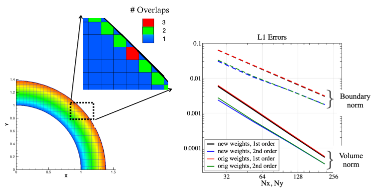
Figure 5: Supersonic vortex test case. Left - density profile of test case. Zoom shows the size of the final updates ($N_{i}$). On this mesh only one cell has update size 3, with three cells contributing to its final update $U^{n+1}$. Right - convergence results for normal merging, comparing the new weights and the original weights, with both first order and second order accurate gradient reconstruction. Both the volume norm and boundary norm of the errors are presented.

Fig. 5 shows the L1 norm of the volume error in density (solid lines) and the L1 boundary norm (dashed lines), defined as the sum of the absolute value of the errors in each cut cell times its boundary segment length. As in [6] the overall convergence rate is second order, and the boundary norms converges at somewhat less than 1.5. However the second order errors are half that of the first order errors, at very little additional cost. The new monotone weights are very slightly better than the original weights on coarser grids, but not noticeable on finer grids when they are hidden behind other errors that come to dominate in the solution. In [6] the comparison used central merging. This is much more diffusive, and a bigger difference between the weights was observed than in this normal merging case.

5.2 Shock diffraction

Since once of the reasons for monotonicity is to robustly handle shocks, the next example shows shock diffraction around a crescent shape, so there is both a concave and convex boundary. The domain is $[\sm 1.60.4]\times[\sm 1,1]$. The mesh spacing is chosen so that the tips of the crescent are located at a gridpoint, so that each refinement still sees the same geometry except for the last cell. Since the geometry is thin at the corners, care must be taken to not include points on the opposite side in the gradient stencils. For this reason we use first order accurate gradients with a 3-by-3 stencil. Since we use normal merging, there is no danger of including cells from the other side in forming neighborhoods. In this example all cut cells only merge with one neighbor, and all final updates include at most one other cell. All the neighborhood and update sizes are 2 or less in this case. The initial conditions are a Mach 2 shock approaching from the right, as shown in Fig. 6 left. The solution at time 0.7 is shown on the right. We use the 2 stage Runge-Kutta time stepper with a CFL = 0.5. A plot showing convergence of density around the surface is in Fig. 7, going from 200 to 1600 points in each dimension. The last two data sets, with 800 and 1600 points, are essentially on top of each other away from the singular corner. The smallest volume fraction in the 1600 cell mesh was $2.6\times 10^{\sm 17}$, occurring in two cells.

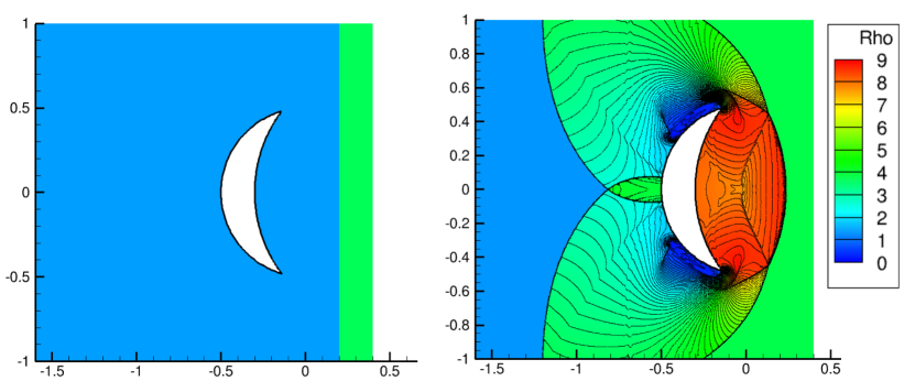
Figure 6: Shock reflection from a crescent. Left figure shows the initial conditions of a Mach 2 shock traveling to the left. Right shows density at time 0.7.

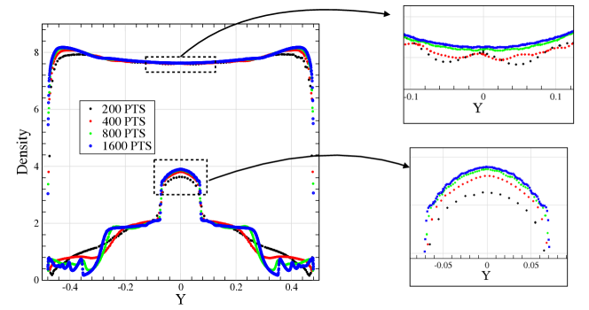
Figure 7: Plot of density along the boundary of the geometry. The solution at the boundary is reconstructed from the cell centers using first order gradients described in the text. Zooms show the finest two solutions away from the corners are very close.

5.3 Acoustic pulse through trefoil

In this example, we compute the scattering of an acoustic pulse by solving the Euler equations inside a trefoil-shaped cavity. The purpose of this example is to show that the weights behave well in 3D curved geometry too, although the analysis uses planar geometry. The surface of this complex geometry is meshed with 47,396 flat triangles using Mathematica [10] from a level set definition [12]:

(31) $$u(x,y,z) =\frac{2(x+yi)}{1+x^{2}+y^{2}+z^{2}},$$

$$v(x,y,z) =\frac{2z+i(x^{2}+y^{2}+z^{2}-1)}{1+x^{2}+y^{2}+z^{2}},$$

$$\Psi(x,y,z) =\left|\frac{u(x,y,z)^{3}}{u(x,y,z)^{3}+v(x,y,z)^{2}}\right|,$$

where $i$ is the imaginary number, and $|\cdot|$ is the magnitude of the complex argument. The trefoil cavity used in this example is given by the implicit equation $\Psi(x,y,z)\geq 1.01$.

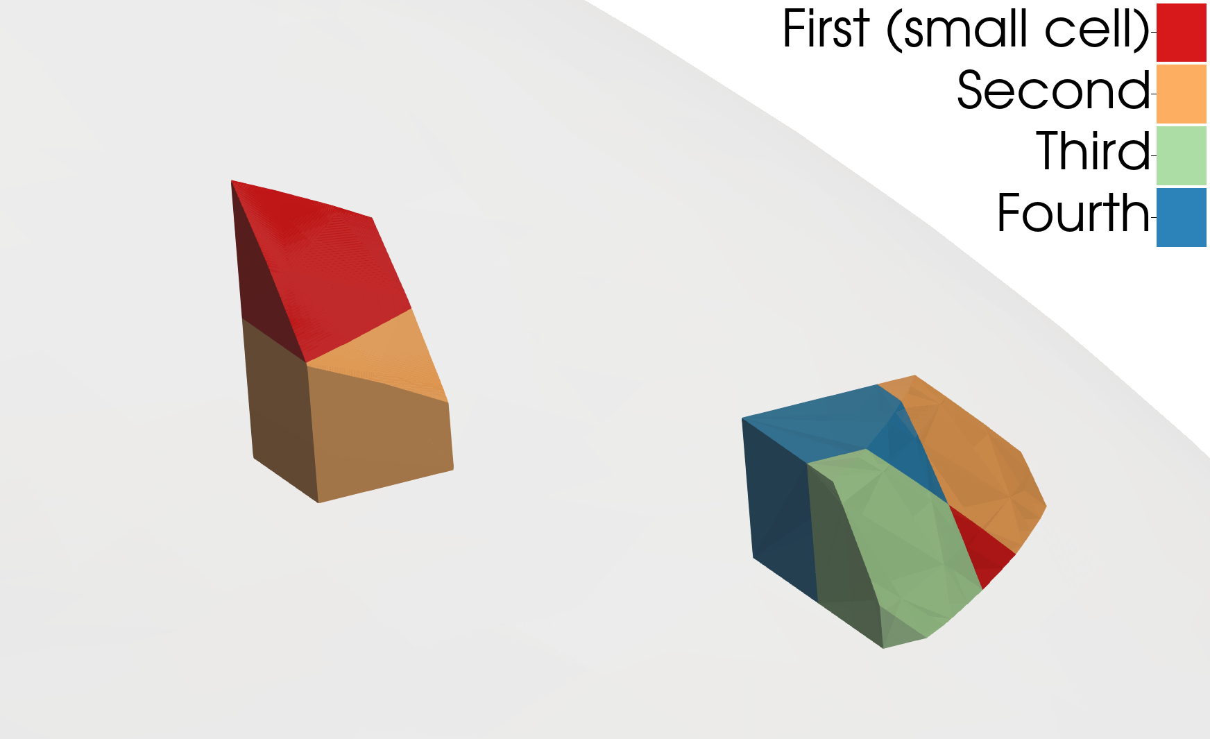
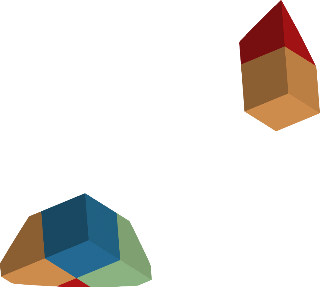
Figure 8: Two possible overlap count configurations in three dimensions seen from outside the trefoil looking in (left), and vice versa (right). The small cell with volume fraction less than $V_{\text{target}}=1/2$ is colored in red. Subsequent cells added to neighborhood are colored according to the legend. The first neighborhood has only two cells shows standard normal merging. The other neighborhood has four cells, since the first and second cells in the neighborhood do not have a large enough volume fraction. Thus, the third cell is added, along with the fourth to prevent “L”-shaped neighborhoods.

The cut cell mesh is obtained from an $79\times 79\times 79$ background Cartesian grid on the domain $[\sm 2.25651,3.09301]\times[\sm 2.67476,2.67476]\times[\sm 2.67476,2.67476]$. There are 30,874 whole Cartesian cells, 16,983 cut cells in the mesh, and the minimum cut cell volume fraction stabilized by state redistribution is 1.19e-13. The complex boundary is first meshed using flat triangles, then this surface mesh is given to the Mandoline mesh generator [14] to obtain the three-dimensional embedded boundary grid.

The formula for monotone weights used in the 2D analysis of Section 4 directly extends to three dimensions and are used here. Each merging neighborhood is generated using the normal merging strategy proposed in [6], with a merging tolerance of $V_{\text{target}}=1/2$. On this geometry, merging a small cell with a face neighbor that is closest the inward pointing boundary normal will not necessarily result in a neighborhood volume larger than $V_{\text{target}}=1/2$. However, more than 92% of the time, standard normal was sufficient as shown in Table 1 (right). One solution to this problem is to first merge in the direction of the largest component of the inward pointing normal. If this neighborhood size is insufficient, then the cell in the direction of the next largest component of the normal is added. Then, a fourth cell is added to prevent “L”-shaped neighborhoods, see the supplementary materials or Fig. 8 for an illustration of this kind of neighborhood. The overlap counts, neighborhood sizes, and associated frequencies in the cut cell mesh are provided in Table 1. The merging strategy used is the reason that we do not observe neighborhoods with 3 cells. Most cells have overlap counts of 1 and 2, but the overlap count can be as large as 7. This is much larger than what we generally observe in two dimensions, where overlap counts usually range between 1 and 3. Two possible overlap configurations are shown in Fig. 8.

final update size $|W_{i}|$	frequency
1	39421
2	6839
3	1263
4	286
5	37
6	6
7	5

merging neighborhood size $|M_{i}|$	frequency
1	38738
2	8463
3	0
4	656

Table 1: Frequencies of final update size, and neighborhood sizes in the trefoil cut cell mesh, where the background Cartesian grid is $80\times 80\times 80$.

The initial condition is given by

$$\begin{pmatrix}\rho\\ u\\ v\\ P\end{pmatrix}=\begin{pmatrix}1-1/\gamma+P\\ 0\\ 0\\ 1/\gamma+10^{\sm 4}\exp(-b\left[(x-x^{*})^{2}+(y-y^{*})^{2}+(z-z^{*})^{2}\right])\end{pmatrix},$$

where $\gamma=1.4$, $b=\text{log}(2)/10^{2}$, and $(x^{*},y^{*},z^{*})=(1.91867,0.13616,0)$ centers the Gaussian perturbation inside the cavity. No shocks develop since this is a low amplitude perturbation. Thus, we do not limit and use the full $\text{CFL}=1$. We reconstruct first order accurate gradients in primitive variables without limiting. Isobars and slices of the numerical solution are plotted at various times in Fig. 9, where we observe that the solution is smooth up to the embedded boundary.

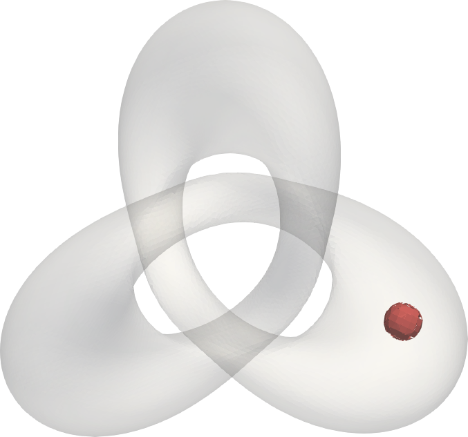
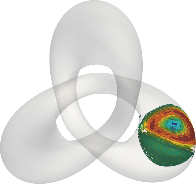
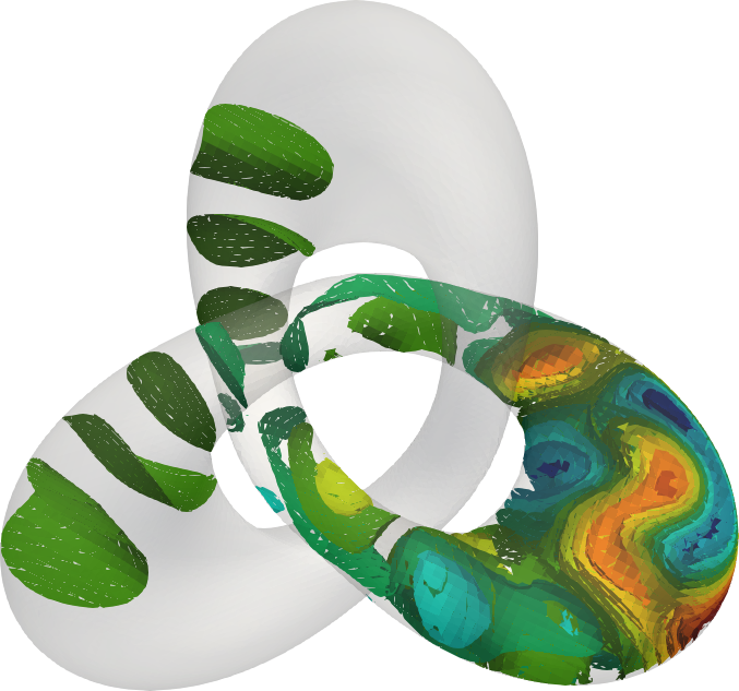
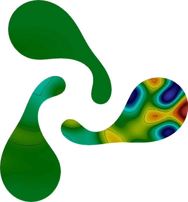
Figure 9: Scattering of acoustic pulse in trefoil cavity. The trefoil embedded boundary is transparent and encloses the computational domain. From left to right, each column shows the pressure difference $(P-1/\gamma)/10^{\sm 4}$ in the numerical solution at times $t=0,2\Delta t$ and $22\Delta t$. The top row corresponds to isosurfaces in the pressure difference, while the bottom row shows a slice with isolines on the $z=0.2$ plane. The amplitude of the pressure pulse decays quickly, so the color scales in each image are not necessarily the same.

6 Conclusions

We have proposed a family of weights that generalizes the original State Redistribution algorithm. The original weights were defined using only the number of neighbors of a cut cell. The new weights include the volume fraction, and shut off smoothly as it approaches the target volume We have analyzed some stability properties of both the new and old SRD weights. The newest formulation is monotone in most situations that occur in practice. It would be more satisfying to have a general approach that did not rely on specific configurations but we unfortunately did not (yet) find one.

One SRD property that is still lacking is a way to reduce the amount of post-processing when the solution update goes to zero. The original flux redistribution method [4] had this property automatically, since it redistributed only the cell update itself, not the whole state. If the update was zero, e.g. at steady state, nothing changed. Flux stabilization [7] is another approach which takes into account the local CFL number for improved performance at stagnation points, or where the cut cell is large enough to only require a small amount of stabilization. Another useful property might be to write the weights as functions of the local CFL number $\lambda$ instead of maximizing over it.

Appendix A Monotonicity of Linear Advection

In this Appendix we derive the formulas presented in Section 4. As with the 1D example in Section 2 it is necessary to step from the merging neighborhoods $\widehat{Q}^{n-1}$ to $\widehat{Q}^{n}$ rather than from $U^{n-1}$ to $U^{n}$. In other words, the pre-merging step is necessary for monotonicity. It may happen that a particular configuration has positive coefficients without pre-merging but it does not always carry over to parallel flow in the opposite direction (as in the 1D case where merging right works without pre-merging but merging left does not).

A.1 Derivation of $\widehat{Q}$ Update Formula

First we show that the neighborhood average $\widehat{Q}^{n}_{j}$ can be written as a convex combination of the merging neighborhoods $\widehat{Q}^{n-1}_{j}$ at time $n-1$. We will look in detail at the contribution of neighborhood average $\widehat{Q}_{j}$ on cell $j$ to cell average $U_{i}$ for cell $i$, for $j\in W_{i}$. We have

(32) $$U_{i}^{n} =\sum_{m\in W_{i}}\;w_{i,m}\widehat{Q}_{m}^{n-1}$$

$$=w_{i,j}\,\widehat{Q}_{j}^{n-1}+\sum_{m\in W_{i},m\neq j}\;w_{i,m}\widehat{Q}_{m}^{n-1}$$

$$=w_{i,j}\,\widehat{Q}_{j}^{n-1}\;+\;(1-w_{i,j})\,\widetilde{Q}_{i}^{n-1}$$

where we define

(33) $$\widetilde{Q}_{i}^{n-1}=\frac{1}{1-w_{i,j}}\,\sum_{m\in W_{i},m\neq j}\;w_{i,m}\widehat{Q}_{m}^{n-1}.$$

The $\widetilde{Q}^{n-1}_{i}$ are the rest of the neighborhoods that contribute to cell $i$, excluding cell $j$. For a concrete example, suppose we have three cells, $C_{\sm 1},C_{0}$ and $C_{1}$, with $i=0$, $j=\sm 1$, we can write

(34) $$U^{n}_{0} =w_{0,\sm 1}\widehat{Q}^{n-1}_{\sm 1}+w_{0,1}\widehat{Q}^{n-1}_{1}+w_{0,0}\widehat{Q}^{n-1}_{0}$$

$$=w_{0,\sm 1}\widehat{Q}^{n-1}_{\sm 1}+(1-w_{0,\sm 1})\frac{(w_{0,1}\widehat{Q}^{n-1}_{1}+w_{0,0}\widehat{Q}^{n-1}_{0})}{(1-w_{0,\sm 1})}$$

$$=w_{0,\sm 1}\widehat{Q}^{n-1}_{\sm 1}+(1-w_{0,\sm 1})\widetilde{Q}^{n-1}_{0}$$

Note that $\widetilde{Q}^{n-1}_{0}$ itself is also a convex combination of neighborhoods and weights that sum to 1, since $w_{0,1}+w_{0,0}=1-w_{0,\sm 1}$.

Next we go from $U^{n}$ to $\widehat{U}^{n}$, pulling out the inflow states for linear advection. In 2D (also generalizes to 3D), an update can be written:

(35) $$\widehat{U}^{n}_{i} =\left(1-\frac{\Delta t}{V_{i}}\sum_{k\in\text{outflow}_{i}}l_{i,k}h\,\mathbf{a}\cdot\mathbf{n}_{i,k}\right)\,U^{n}_{i}+\frac{\Delta t}{V_{i}}\sum_{k\in\text{inflow}_{i}}l_{i,k}h\,\mathbf{a}\cdot\mathbf{n}_{k,i}\,U^{n}_{k}$$

$$=\left(1-\frac{\Delta t\,h}{V_{i}}\sum_{k\in\text{inflow}_{i}}l_{i,k}|\mathbf{a}\cdot\mathbf{n}_{i,k}|\right)\,U^{n}_{i}+\frac{\Delta t\,h}{V_{i}}\sum_{k\in\text{inflow}_{i}}l_{i,k}|\mathbf{a}\cdot\mathbf{n}_{i,k}|\,U^{n}_{k},$$

where $l_{i,k}h$ is the length of the edge between cells $i$ and $k$, $\text{inflow}_{i}$ is the set of cell indices that are inflow with respect to cell $i$, and $\mathbf{a}$ is the advection velocity. Here we have used the divergence theorem $\sum_{k\in\{cell\,i\,faces\}}\,l_{i,k}\,\mathbf{a}\cdot\mathbf{n}_{i,k}\,=0$ to write everything in terms of inflow faces and normals and take absolute values.

Putting $\Delta t$ inside the sums and replacing $V_{i}=\alpha_{i}h^{2}$, (35) becomes

(36) $$\widehat{U}^{n}_{i} =\left(1-\frac{h}{V_{i}}\sum_{k\in\text{inflow}_{i}}\Delta t\,l_{i,k}|\mathbf{a}\cdot\mathbf{n}_{i,k}|\right)\,U^{n}_{i}+\frac{h}{V_{i}}\sum_{k\in\text{inflow}_{i}}\Delta t\,l_{i,k}|\mathbf{a}\cdot\mathbf{n}_{i,k}|\,U^{n}_{k}$$

$$=\left(1-\frac{\lambda_{i}}{\alpha_{i}}\right)U^{n}_{i}+\sum_{k\in\text{inflow}_{i}}\frac{\lambda_{i,k}}{\alpha_{i}}U^{n}_{k}.$$

where we use the notation $\lambda_{i}=\sum_{k\in\text{inflow}_{i}}\lambda_{i,k}$ where $\lambda_{i,k}=\Delta t~{}l_{i,k}|\mathbf{a}\cdot\mathbf{n}_{i,k}|/h$.

The final step to go from the finite volume update $\widehat{U}^{n}$ to the merging neighborhoods $\widehat{Q}^{n}$. After multiplying both sides of (21) by $\widehat{V}_{j}/h^{2}$ we get

(37) $$\frac{\widehat{V}_{j}}{h^{2}}\widehat{Q}^{n}_{j}=\sum_{i\in M_{j}}w_{i,j}\alpha_{i}\widehat{U}^{n}_{i}$$

After some routine algebra pre-multiplying $\widehat{U}^{n}_{i}$ in (36) by $w_{i,j}\alpha_{i}$, substituting into (37), and using (32) to replace the ${U^{n}}$ terms, we finally get the expression for the $\widehat{Q}$ updates in terms of those from the previous step,

(38) $$\frac{\widehat{V}_{j}}{h^{2}}\widehat{Q}^{n}_{j} =\sum_{i\in M_{j}}\left(w_{i,j}^{2}(\alpha_{i}-\lambda_{i})+w_{i,j}\sum_{k\in\text{inflow}_{i}}w_{k,j}\lambda_{i,k}\right)\widehat{Q}^{n-1}_{j}$$

$$+\,(w_{i,j}-w_{i,j}^{2})(\alpha_{i}-\lambda_{i})\;\widetilde{Q}^{n-1}_{i}$$

$$+\,w_{i,j}\sum_{k\in\text{inflow}_{i}}\lambda_{i,k}\left(1-w_{k,j}\right)\,\widetilde{Q}^{n-1}_{k}$$

This is the fully general formula that holds in 1, 2 and 3 dimensions with appropriate changes to areas and volumes. In the next subsection we apply this formula to normal merging configurations in 2D, where the formulas simplify greatly.

A.2 Proof of Monotonicity

Here we adapt formula (38) to the two 2D configurations that can result from normal merging to show the coefficients are positive. Additional configurations are in the supplementary materials. We prove monotonicity for ramp angles less than $45^{\circ}$ with vertical merging. Monotonicity for greater ramp angles and horizontal merging can be shown by rotating the configuration $90^{\circ}$ clockwise and flipping it horizontally, resulting in this case but with negative velocity.

A.2.1 Normal Merging

In 2D there are two cases for normal merging, illustrated in Fig. 10 (as in Fig. 3 but with more notation). In both cases the merging neighborhoods contain only two cells from the base grid, and the formulas greatly simplify.

[width=0.3 ]images/2D_cut_square/2D_1   [width=0.3 ]images/2D_cut_square/2D_2

Figure 10: Notation for the two possible configurations in 2D with SRD using normal merging and flow parallel to a planar boundary.

Let cell $0$ be the index of the small cell and cell $1$ is the large cell that it merges with. In both cases we must have $w_{0,0}=1$, since no other neighborhoods besides its own contain cell 0. The inflow cell for cell 0 is only cell 2. The inflow cells for cell 1 are cell 0 and 5.

For these two cells, (38) becomes

(39) $$\frac{\widehat{V}_{0}}{h^{2}}\widehat{Q}^{n}_{0}= \left(\alpha_{0}-\lambda_{0}+w_{1,0}^{2}(\alpha_{1}-\lambda_{1})+w_{1,0}\lambda_{1,0}\right)\widehat{Q}^{n-1}_{0}\,+$$

$$\,(w_{1,0}-w_{1,0}^{2})(\alpha_{1}-\lambda_{1})\widehat{Q}^{n-1}_{1}+\lambda_{0,2}\widehat{Q}^{n-1}_{2}+w_{1,0}\lambda_{1,5}\,\widetilde{Q}^{n-1}_{5}$$

$$\frac{\widehat{V}_{1}}{h^{2}}\widehat{Q}^{n}_{1} =w_{1,1}^{2}(\alpha_{1}-\lambda_{1})\widehat{Q}^{n-1}_{1}+\,\left[(w_{1,1}-w_{1,1}^{2})(\alpha_{1}-\lambda_{1})+w_{1,1}\lambda_{1,0}\right]\;\widehat{Q}^{n-1}_{0}+$$

$$+w_{1,1}\lambda_{1,5}\,\widetilde{Q}^{n-1}_{5}$$

In both configurations cell 1 has not been merged since it has volume fraction $\alpha_{1}\geq 0.5$. Since there is only one inflow cell face for cell 1 that is different from cell 0, the definition of $\lambda_{1}$ simplifies to $\lambda_{1,5}=\Delta t\,l_{1,5}a/h$, where the length $l_{1,5}\leq 1$ and $a$ is the $x$-component of the velocity $\mathbf{a}$. The term $\widetilde{Q}_{5}^{n-1}$ represents the neighborhood contributing to cell 5, which might include cell 2 along with cell 5 itself. However since the coefficient in front of this term is positive it does not play a role in determining the monotonicity of the update. It can be shown that the term $\alpha_{1}-\lambda_{1}$ in both equations is positive in both configurations if you take a stable time step on the full Cartesian cells in the base grid satisfying (23).

Thus in (39) the only possibly negative coefficient is in front of $\widehat{Q}_{0}^{n-1}$ in the first equation. We must find a weight $w_{1,0}$ such that

(40) $$\alpha_{0}-\lambda_{0}+w_{1,0}^{2}(\alpha_{1}-\lambda_{1})+w_{1,0}\ \lambda_{1,0}\geq 0.$$

For flow down the ramp with velocity $-\mathbf{a}$, the same inequality results.

Configuration 1:

We can take the velocity to be $\mathbf{a}=[1,l_{0,2}-l_{0,3}]$, which is parallel to the embedded boundary. Since $\Delta t$ satisfies $\Delta t\cdot(1/h+(l_{0,2}-l_{0,3})/h)=\text{CFL}\leq 1$, the velocity magnitude does not affect this analysis. For this case we have the volume fraction $\alpha_{1}=1$ (the cell is not cut), and $\lambda_{1}=\frac{\Delta t}{h^{2}}\cdot(h+(l_{0,2}-l_{0,3})\cdot h)$. This gives $\alpha_{1}-\lambda_{1}\geq 0$, and is zero if the maximum time step is taken on the base grid. Thus it is sufficient that $w_{1,0}$ satisfy

$$\alpha_{0}-\lambda_{0}+w_{1,0}\lambda_{1,0}\geq 0.$$

Solving for the weight, we obtain

(41) $$\frac{\lambda_{0}-\alpha_{0}}{\lambda_{1,0}}\leq w_{1,0}.$$

The left hand side of this inequality depends on the geometry and flow angle of the channel. We want this estimate to hold for all flow angles less than $45^{\circ}$, which we can exactly calculate. Referencing Fig. 10, we define the left and right vertical edges of cell 0 to have edge fraction $0\leq l_{0,2},l_{0,3}\leq 1$, $l_{0,2}>l_{0,3}$. The linear advection problem is now completely defined. We can then evaluate

(42) $$\alpha_{0} =\frac{1}{2}(l_{0,2}+l_{0,3})$$

$$\lambda_{0} =\Delta t\frac{l_{0,2}}{h},\;\;\lambda_{1,0}=\Delta t\frac{l_{0,2}-l_{0,3}}{h}$$

It’s easiest to analyze with the maximum stable time step, which we do next. Substituting everything into the left hand side of the inequality (41), we obtain

(43) $$\frac{\lambda_{0}-\alpha_{0}}{\lambda_{1,0}} =\frac{l_{0,2}-l_{0,3}-(l_{0,2}^{2}-l_{0,3}^{2})}{2\,(l_{0,2}-l_{0,3})}=\frac{1}{2}-\frac{1}{2}(l_{0,2}+l_{0,3})$$

$$=\frac{1}{2}-\alpha_{0}\;\leq w_{1,0}\;\leq\,1.$$

We have also verified by differentiating with respect to the CFL number that this maximizes the left hand side.

Summarizing, this shows that for this case where $\alpha_{0}<0.5$ both the original SRD weights, where $w_{1,0}=1/2$, and the new monotone weights from (22), with $w_{1,1}=2\alpha_{0},w_{1,0}=1-2\alpha_{0}$, satisfy inequality (43). This helps explain the good performance of the original SRD algorithm in this common configuration. For the previously mentioned $\alpha\beta$ scheme, configuration 1 results in weight $w_{1,0}=\frac{1}{2}(\frac{1}{2}-\alpha_{0})$, which does not satisfy (43), but may satisfy (40) depending on the time step.

Configuration 2:

The advection velocity is now $\mathbf{a}=[1,l_{0,2}+1-l_{1,4}]$ and $0\leq l_{0,2},l_{1,4}\leq 1$. Requiring ramp angles less than $45^{\circ}$ implies $l_{0,2}+1-l_{1,4}\leq 1$. The parameters are:

(44) $$\alpha_{0} =\frac{1}{2}\,\frac{l_{0,2}^{2}}{l_{0,2}+1-l_{1,4}}\text{ and }\alpha_{1}=1-\frac{1}{2}\,\frac{(1-l_{1,4})^{2}}{l_{0,2}+1-l_{1,4}}$$

$$\lambda_{0} =\Delta t\frac{l_{0,2}}{h},\;\>\lambda_{1,0}=\Delta t\frac{l_{0,2}}{h}\;\text{ and }\>\lambda_{1}=\Delta t\left(\frac{1}{h}+\frac{l_{0,2}}{h}\right)$$

$$\Delta t \left(\frac{1}{h}+\frac{l_{0,2}+1-l_{1,4}}{h}\right)=\text{CFL}\in(0,1]$$

Unlike configuration 1, one can show that the multiplier $(\alpha_{1}-\lambda_{1})$ of the quadratic term in (40) is a positive number, and is zero only in special cases such as a 45^∘ channel where both $l_{0,2}$ and $l_{1,4}=0$, or a horizontal wall.

The quadratic (repeating (40) for convenience)

$$\alpha_{0}-\lambda_{0}+w_{1,0}^{2}(\alpha_{1}-\lambda_{1})+w_{1,0}\ \lambda_{1,0}\geq 0.$$

is concave up with roots $\frac{-\lambda_{1,0}\pm\sqrt{\lambda_{1,0}^{2}-4(\alpha_{1}-\lambda_{1})(\alpha_{0}-\lambda_{0})}}{2(\alpha_{1}-\lambda_{1})}$. The term $\alpha_{0}-\lambda_{0}$ is negative, so the roots of the quadratic are real, with one negative and one positive root. For $w_{1,0}$ to be positive it must be greater than the positive root $r_{+}$, so we require

(45) $$r_{+}=\frac{-\lambda_{1,0}+\sqrt{\lambda_{1,0}^{2}-4(\alpha_{1}-\lambda_{1})(\alpha_{0}-\lambda_{0})}}{2(\alpha_{1}-\lambda_{1})}\leq w_{1,0}.$$

After substituting in the information from (44) we get a complicated expression that is a function of $l_{0,2}$, $l_{1,4}$, and the CFL number. We find that for an appropriately chosen time step, we can still get

(46) $$r_{+}=\frac{-\lambda_{1,0}+\sqrt{\lambda_{1,0}^{2}-4(\alpha_{1}-\lambda_{1})(\alpha_{0}-\lambda_{0})}}{2(\alpha_{1}-\lambda_{1})}\leq\,\frac{1}{2}-\alpha_{0}\,\leq w_{1,0}.$$

but the CFL must be slightly less than 1. Estimating numerically we find that a $\text{CFL}\leq 0.92$ is sufficient. This is illustrated graphically in Fig. 11.

Figure 11: $r_{+}$ and $1/2-\alpha_{0}$ are plotted with respect to edge fractions $l_{0,2},l_{1,4}$, when $\text{CFL}=1$ and $\text{CFL}=0.92$ on the left and right, respectively. These functions are only plotted on the gray triangular region of configuration 2 where $l_{0,2}+1-l_{1,4}\leq 1$ for $0\leq l_{0,2},l_{1,4}\leq 1$. Left shows the non-monotone region where $r_{+}>1/2-\alpha_{0}$ so (46) is not satisfied. For CFL $\leq 0.92$ the monotonicity requirement is met.

This shows that provided a slightly smaller time step is chosen, the original SRD scheme is monotone! If a full $\text{CFL}=1$ is taken, there are negative coefficients, and monotonicity cannot be guaranteed, although it takes a well constructed example to observe it.

Summarizing, we have shown that any weight that satisfies

(47) $$1/2-\alpha_{0}\leq w_{1,0}\leq 1$$

will result in a monotone scheme when taking a $\text{CFL}\leq 0.92$. Our fully general set of weights in (22) when specialized to normal merging in configuration 1 or 2 become

(48) $$w_{1,0}=1-2\alpha_{0}\text{ and }w_{1,1}=2\alpha_{0},$$

when the overlap count is 2 on cell 1 as in Fig. 3.

Appendix B Stability of Original SRD for 1D Model Problem

This section proves the claim (with the help of a plot) from Section 2 that both the original and new monotone SRD weights are stable in the sense of GKS [9] for the model problem with one small cell. We use a merging left neighborhood and no pre-merging, We are looking at linear advection and the first order upwind scheme, which simplifies the analysis a lot. We assume the interested reader is familiar with GKS theory and do not go into detail here.

When written as a one step formula, the updates for merging left are given by (8). The GKS analysis reduces to checking whether these two cells can grow in time with an amplification factor $z\geq 1$. We transform in time, using the variable $z$, and use constants $c$ and $d$ for the characteristic values for $U_{\sm 1}$ and $U_{0}$. We simplify the notation and use $w$ for $w_{\sm 1,\sm 1}$ and replace $w_{\sm 1,0}=1-w$. We get to set the characteristic value for $U_{\sm 2}=0$), and we end up with the equations

(49) $$z\,c =\frac{(1-w+\alpha\,w-\alpha\lambda w)}{\widehat{V}_{0}}\,c+\frac{(1-w)\,(\alpha-\lambda)}{\widehat{V}_{0}}\,d$$

$$z\,d =\frac{(\lambda+(1-w)\,(1-\lambda))}{\widehat{V}_{0}}\>c\>+\>\frac{(\alpha-\lambda)}{\widehat{V}_{0}}\,d$$

In matrix form, this is

(50) $$\begin{pmatrix}z-\frac{(1-w+\alpha w-\alpha\lambda w)}{\widehat{V}_{0}}&\frac{-(1-w)(\alpha-\lambda)}{\widehat{V}_{0})}\\[5.78172pt] \frac{-(\lambda+(1-w)(1-\lambda))}{\widehat{V}_{0}}&z-\frac{(\alpha-\lambda)}{\widehat{V}_{0}}\end{pmatrix}\begin{pmatrix}c\\[5.78172pt] d\end{pmatrix}=\begin{pmatrix}0\\[5.78172pt] 0\end{pmatrix}$$

The determinant of the matrix gives a quadratic polynomial in $z$. The scheme is stable if there are no values of $|z|>1$ where the determinant of (50) = 0, and no borderline cases with $|z|=1$.

In the two cases of interest, the original SRD weights for the model problem set $w=1/2$. The new monotone weights use $w=\alpha$. Fig. 12 plots the maximum absolute value of the two roots as a function of the CFL number $\lambda$, for several small cell fractions $\alpha<0.5$. The values are clearly below 1. It is easy to show analytically that the extremum values of $\alpha=0,\lambda=1$ are stable, and the plots show the direction that $|z|$ moves in for the other values.

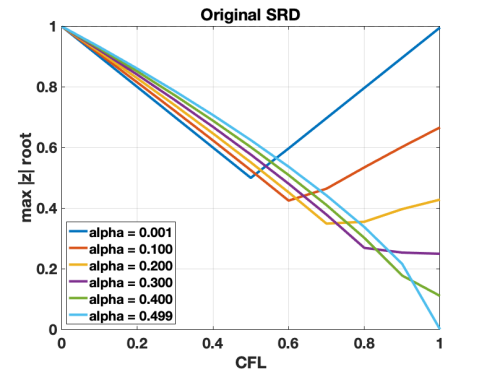
Figure 12: Maximum root of GKS determinant is $\leq 1$ for the model problem with one small cell. Left figure shows the original weights ($w=1/2$), right shows the monotone weights ($w=\alpha$). All growth is bounded by 1, showing stability of both original and weighted SRD merging left and without pre-merging, although they are not monotone.

References

- [1] M. Aftosmis, D. Gaitonde, and T. S. Tavares, On the accuracy, stability and monotonicity of various reconstruction algorithms for unstructured meshes, AIAA-94-0415, (1994).
- [2] M. Berger and A. Giuliani, A state redistribution algorithm for finite volume schemes on cut cell meshes, Journal of Computational Physics, 428 (2021), p. 109820.
- [3] M. J. Berger, C. Helzel, and R. J. LeVeque, H-box methods for the approximation of one-dimensional conservation laws on irregular grids, SIAM J. Numer. Anal., 41 (2003), pp. 893–918.
- [4] I. Chern and P. Colella, A conservative front tracking method for hyperbolic conservation laws, Tech. Report UCRL-97200, Lawrence Livermore National Laboratory, July 1987.
- [5] C. Engwer, S. May, A. Nüßing, and F. Streitbürger, A stabilized DG cut cell method for discretizing the linear transport equation, SIAM Journal on Scientific Computing, 42 (2020), pp. A3677–A3703.
- [6] A. Giuliani, A. Almgren, J. Bell, M. Berger, M. Henry de Frahan, and D. Rangarajan, A weighted state redistribution algorithm for embedded boundary grids, Journal of Computational Physics, 464 (2022), p. 111305, https://doi.org/https://doi.org/10.1016/j.jcp.2022.111305, https://www.sciencedirect.com/science/article/pii/S0021999122003679.
- [7] N. Gokhale, N. Nikiforakis, and R. Klein, A dimensionally split Cartesian cut cell method for hyperbolic conservation laws, Journal of Computational Physics, 364 (2018), pp. 186–208, https://doi.org/https://doi.org/10.1016/j.jcp.2018.03.005, https://www.sciencedirect.com/science/article/pii/S0021999118301578.
- [8] S. Gottlieb, C.-W. Shu, and E. Tadmor, Strong stability-preserving high-order time discretization methods, SIAM review, 43 (2001), pp. 89–112.
- [9] B. Gustafsson, H.-O. Kreiss, and A. Sundström, Stability theory of difference approximations for mixed initial boundary value problems. II, Math. Comp., 26 (1972), pp. 649–686.
- [10] W. R. Inc., Mathematica, Version 13.3, https://www.wolfram.com/mathematica. Champaign, IL, 2023.
- [11] H. Ji, F. S. Lien, and E. Yee, Numerical simulation of detonation using an adaptive Cartesian cut-cell method combined with a cell-merging technique, Computers & Fluids, 39 (2010), pp. 1041–1057.
- [12] H. Kedia, D. Foster, M. R. Dennis, and W. T. Irvine, Weaving knotted vector fields with tunable helicity, Physical review letters, 117 (2016), p. 274501.
- [13] R. Saye, Implicit mesh discontinuous Galerkin methods and interfacial gauge methods for high-order accurate interface dynamics, with applications to surface tension dynamics, rigid body fluid–structure interaction, and free surface flow: Part i, Journal of Computational Physics, 344 (2017), pp. 647–682.
- [14] M. Tao, C. Batty, E. Fiume, and D. Levin, Mandoline: Robust cut-cell generation for arbitrary triangle meshes, ACM Transactions on Graphics, (2019).
- [15] C. Taylor and J. Chan, Energy stable state redistribution cut-cell DG methods for wave propagation, https://meetings.siam.org/sess/dsp_talk.cfm?p=124718. Talk given at the 2023 SIAM Conference on Computational Science and Engineering.