Canonical typicality under general quantum channels

Abstract

With the control of ever more complex quantum systems becoming a reality, new scenarios are emerging where generalizations of the most foundational aspects of statistical quantum mechanics are imperative. In such experimental scenarios the often natural correspondence between the particles that compose the system and the relevant degrees-of-freedom might not be observed. In the present work we employ quantum channels to define generalized subsystems, which should capture the pertinent degrees-of-freedom, and obtain their associated canonical state. Moreover, we show that generalized subsystems also display the phenomena of canonical typicality, i.e., the generalized subsystem description generated from almost any microscopic pure state of the whole system will behave similarly as the corresponding canonical state. In particular we demonstrate that the property regulating the emergence of the canonical typicality behavior is the entropy of the channel used to define the generalized subsystem.

Introduction. Ensembles form an integral part of statistical mechanics, being key ingredients in pillar fields as thermodynamics and statistical mechanics (both classical and quantum). An ensemble formalizes the idea that for complex systems one cannot control all its degrees-of-freedom as to prepare it in a well-defined state. In each run of the experiment only few “macroscopic” quantities are fixed, and thus any of the “microscopic” states that are consistent with the macroscopic quantities can be prepared. The collection of such compatible microscopic states forms the statistical ensemble of a given experimental scenario.

Two of the most prevailing ensembles in physics are the microcanonical and the canonical ensembles. For the first we imagine a scenario where the system is formed by a large number of degrees-of-freedom which are completely isolated from the rest of the universe, with some macroscopic properties having well-defined values. For the second, the canonical ensemble can be seen as the description of a subsystem, with fixed number of degrees-of-freedom, of the microcanonical one. The canonical ensemble thus characterize the situation where macroscopic properties are allowed to vary within a given subsystem, while such properties are fixed when considering the whole system.

While the use of ensembles has been very successful, they introduce a probabilistic character to the microscopic description, which can be argued deterministic. Indeed, in a given run of an experiment one might expect that all properties of the probed system are fixed, and not just the few controlled macroscopic quantities. Within this reasoning, the microscopic state is well defined, albeit unknown. To reconcile this deterministic perspective with the overwhelming success of the probabilistic description is one of the main discussions in the foundations of statistical mechanics since Boltzmann. The most common justification, using the microscopic laws of mechanics, invokes chaos theory and the ergodic hypothesis [1]. Others consider an information theory approach, exploiting the principle of maximum entropy as championed by Jaynes [2, 3].

Another possibility is the so-called typicality argument: almost all microscopic states which are compatible with a given preparation procedure will behave similarly to the ensemble description for any macroscopic property [1]. Such a method had been already proposed by Boltzmann, and it was latter extended to the quantum domain by von Neumann [4]. The latter has remained forgotten until the recent reanalysis of the typicality argument from the quantum information perspective [5, 6]. In this modern mindset, the canonical typicality asserts that any pure state from the whole system, that abides by the fixed macroscopic quantities defining a preparation scheme, will be locally, i.e., for the subsystem, close to the canonical state. How close in this perspective will depend on various ingredients and are somehow a formalization of the “thermodynamical limit” (see details below).

Crucial in the above discussion is the concept of a subsystem with a fixed number of degrees-of-freedom. Usually we equate this with the idea of a fixed number of particles, which is a very natural attitude when dealing, for instance, with a gas of weakly interacting atoms. However, there are situations where this identification is not so clear or appropriate. Think for instance of an optical lattice where individual atoms are loaded onto potential wells [7, 8], but their reading is done in blocks that contains multiple wells: In this case a coarse-grained description is more convenient [9, 10]. Another example is that of a superconducting metal described by the BCS theory, with Cooper pairs forming individual entities which are delocalized in space: here the quasi-particle description is more relevant [11]. In these cases, and many others, a more pertinent description is that of a generalized subsystem [12]. It is not the presumed degrees-of-freedom or the real space distribution of them which gives the more fitting account of a subsystem.

In what follows, we employ the theory of quantum channels to define generalized subsystems to and their canonical ensemble. Moreover, we show that such general scenarios also admit a canonical typicality reasoning. In this way we extend the typicality approach to the foundations of statistical mechanics over situations where the description of a physical scenario in terms of its underlying particles is not necessarily the most suitable one. The “thermodynamics” of a given experimental scenario thus depends on what can be measured, i.e., on what can be called an effective particle.

Canonical typicality. We start by briefly reviewing the main ingredients and results of canonical typicality for the case in which the subsystem is just a subset of the total system [5, 13]. Consider a total system to which we assign a Hilbert space $\mathcal{H}_{T}$ – such a space can, for instance, be constructed by the tensor product of $N$ individual particles’ spaces. To define a subsystem we split the total space in two parts, $\mathcal{H}_{T}=\mathcal{H}_{S}\otimes\mathcal{H}_{E}$; the first part, $\mathcal{H}_{S}$, is associated with the subsystem, and $\mathcal{H}_{E}$ is associated with the rest of the system and it is seen as an environment for the subsystem. We then define a restricted subspace $\mathcal{H}_{R}\subseteq\mathcal{H}_{S}\otimes\mathcal{H}_{E}$ in which all the states abide by the macroscopic constraints.

In such a subspace the total system’s description which represents ignorance of any other constraint than the already contemplated by the restriction, is the microcanonical state $\mathcal{E}_{R}=\mathds{1}_{R}/d_{R}$, with $\mathds{1}_{R}$ the projector into $\mathcal{H}_{R}$ and $d_{R}=\dim(\mathcal{H}_{R})$. The system’s canonical state $\Omega_{{\rm tr}_{E}}$ is then obtained by simply discarding the part of the total system which is not related to the subsystem, i.e., by tracing out the environmental degrees of freedom: $\Omega_{{\rm tr}_{E}}={\rm tr}_{E}(\mathcal{E}_{R})$.

The canonical typicality approach is based in showing that for almost all states $\delimiter 69640972\psi\rangle\in\mathcal{H}_{R}$, taken uniformly at random (from the unitarily invariant measure, the Haar measure [14]), the local state of the subsystem, ${\varrho}_{{\rm tr}_{E}}^{\psi}={\rm tr}_{E}(|\psi\rangle\!\langle\psi|)$, is close to the canonical state $\Omega_{{\rm tr}_{E}}$ when the effective dimension of the environment, $d_{E}^{\text{eff}}=1/{\rm tr}(\Omega_{{\rm tr}_{S}}^{2})$ (with $\Omega_{{\rm tr}_{S}}={\rm tr}_{S}(\mathcal{E}_{R})$), is much bigger than the subsystem dimension $d_{S}=\dim(\mathcal{H}_{S})$. Concretely, it was shown that the average distance is bounded as follows:

$$\overline{\mathcal{D}({\varrho}_{{\rm tr}_{E}}^{\psi},\Omega_{{\rm tr}_{E}})}^{\psi}\leq\frac{1}{2}\sqrt{\frac{d_{S}}{d_{E}^{\text{eff}}}}.$$ (1)

In the above, the average is taken over the uniform measure, and $\mathcal{D}({\varrho},\sigma)=\delimiter 69645069{\varrho}-\sigma\delimiter 86422285_{1}/2$ with the trace-norm defined as $\delimiter 69645069A\delimiter 86422285_{1}={\rm tr}\sqrt{A^{\dagger}A}$. Moreover, employing the so-called Levy’s lemma [15, 16] (see Appendix A), the authors showed that the probability for ${\varrho}_{{\rm tr}_{E}}^{\psi}$ being further away from $\Omega_{{\rm tr}_{E}}$ decays exponentially with $d_{R}$. The canonical state is then recovered from any pure state in the restricted subspace when $d_{R}\gg 1$ and $d_{S}\ll d_{E}^{\text{eff}}$, which are then the formal requirements for equilibration.

The canonical typicality principle can thus be seen as a justification for the use of ensembles in statistical mechanics: we do not need to assume ignorance over the whole system to obtain a canonical state for a subsystem, since most pure states of the whole system appear to be in equilibrium when we look locally at a subsystem.

Generalized subsystems. In the above scenario, the subsystem is a simple partition of the pre-established total Hilbert space. Within statistical mechanics it is commonsensical to split the total system into a system of interest, the intended subsystem, and its environment, for which no control is assumed. Such a split is often possible due to the weak interaction between the two parts. By partial tracing the environmental degrees-of-freedom, we obtain the subsystem description.

However, to find a physically motivated partition some reshape the total Hilbert space might be necessary. A text-book example of this is the Hydrogen atom case. A initial description in terms of an electron and a proton is rearranged into the degrees-of-freedom of center-of-mass and relative-particle. In this new split, both effective particles are decoupled and we can solve Schrödinger’s equation. The idea of quasiparticles, ubiquitous in condensed matter physics, is a somewhat more recent example of this reshuffling of Hilbert’ space in order to find meaningful effective descriptions. Once the more compelling degrees-of-freedom are found, the remaining ones can be seen, and treated, as an effective environment.

In the aforementioned cases, the Hilbert space rearrangement was done by a unitary transformation (like Bogoliubov transformations [17]), and the focus on a subsystem was done by tracing out the weakly interacting degrees-of-freedom of the effective environment. In the quantum information lingo, this definition of subsystem is specified by the quantum channel $\Lambda_{{\rm tr}_{E}\circ U}:\mathcal{H}_{T}\mapsto\mathcal{H}_{S}$ which acts as $\Lambda_{{\rm tr}_{E}}^{U}({\varrho})={\rm tr}_{E}(U{\varrho}U^{\dagger})$.

While very useful and successful, this is not the only way to obtain effective subsystems of quantum systems. As established in [12], and further developed in [9, 10, 18, 19, 20, 21, 22, 23], generalized subsystems can be achieved by exploiting the most general form of a quantum channel $\Lambda:\mathcal{L}(\mathcal{H}_{T})\mapsto\mathcal{L}(\mathcal{H}_{S})$ [24]:

$$\Lambda({\varrho})={\rm tr}_{N}(V{\varrho}V^{\dagger}).$$ (2)

In the above expression $V:\mathcal{H}_{T}\mapsto\mathcal{H}_{S}\otimes\mathcal{H}_{N}$ is an isometry. Like unitary transformations, isometries also preserve the scalar product as $V^{\dagger}V=\mathds{1}_{T}$. However, as isometries might change the space dimension, $VV^{\dagger}=\mathds{1}_{SN}$ is a projector onto $\mathcal{H}_{S}\otimes\mathcal{H}_{N}$. It is this very change of dimensions, empowered by the isometry, which can be exploited to obtain generalized subsystems. The total space $\mathcal{H}_{T}$ is reshuffled to $\mathcal{H}_{S}\otimes\mathcal{H}_{N}$, with the space $\mathcal{H}_{N}$ being associated with an effective (possibly mathematically abstract) environment for the generalized subsystem acting on $\mathcal{H}_{S}$. Like before, the now general effective environment is discarded by the partial trace.

A minimal, though instructive, example of a generalized subsystem is as follows [19]. Consider a tree-level atom, with ground state $\delimiter 69640972g\rangle$, and quasi-degenerated excited states $\delimiter 69640972e_{1}\rangle$ and $\delimiter 69640972e_{2}\rangle$. In an experiment where no distinction is made between the excited levels, the atom can be effectively described by a two-level atom. The generalized subsystem is then defined by the map $\Lambda:\mathbb{C}_{3}\mapsto\mathbb{C}_{2}$ whose diagonal entries are $\Lambda(|g\rangle\!\langle g|)=|0\rangle\!\langle 0|$ and $\Lambda(|e_{1}\rangle\!\langle e_{1}|)=\Lambda(|e_{2}\rangle\!\langle e_{2}|)=|1\rangle\!\langle 1|$, with $\delimiter 696409720\rangle$ and $\delimiter 696409721\rangle$ respectively the ground and excited state of the effective two-level atom. Clearly this case cannot be expressed by a unitary transformation followed by a partial trace, as 3 cannot be factorized as 2 times another whole number. It also cannot be seeing as a projection onto a 2-dimensional subspace, for this would not preserve the norm. The full map and isometry for this case is shown in Appendix B. It is important to notice that $V:\mathbb{C}_{3}\mapsto\mathbb{C}_{2}\otimes\mathbb{C}_{2}$, that is, to define this generalized subsystem it was necessary to introduce an artificial, mathematical, environment with dimension 2. This shows the generality and versatility of using quantum channels to define generalized subsystems.

Canonical typicality for generalized subsystems. Here we present the main result of this work, namely that the phenomena of canonical typicality is also achieved for generalized subsystems. In this way, we extend the typicality approach to the foundations of statistical mechanics over a wide range of physical scenarios.

Consider a quantum mechanical system to which we assign a total Hilbert space $\mathcal{H}_{T}$, and suppose that such a system obeys some arbitrary restriction $R$, and thus act on $\mathcal{H}_{R}\subseteq\mathcal{H}_{T}$. If no further constraints are imposed, the description of the system is given by its microcanonical state:

$$\mathcal{E}_{R}=\dfrac{\mathds{1}_{R}}{d_{R}},$$

where $\mathds{1}_{R}$ is the identity (projector) operator in $\mathcal{L}(\mathcal{H}_{R})$, and $d_{R}$ is the dimension of $\mathcal{H}_{R}$. Our generalized canonical state, i.e., the description of the generalized subsystem, will then be given by the action of a general quantum channel $\Lambda:\mathcal{L}(\mathcal{H}_{R})\mapsto\mathcal{L}(\mathcal{H}_{S})$ on the microcanonical state: $\Omega_{\Lambda}:=\Lambda(\mathcal{E}_{R})$.

For the generalized canonical typicality principle we are then interested in showing that for almost any $\delimiter 69640972\psi\rangle\in\mathcal{H}_{R}$, taken uniformly at random, we will have ${\varrho}_{\Lambda}^{\psi}:=\Lambda(|\psi\rangle\!\langle\psi|)\sim\Omega_{\Lambda}$. Following Ref.[5], this is done in two parts.

The first part is to bound the average distance between ${\varrho}_{\Lambda}^{\psi}$ and $\Omega_{\Lambda}$. In Appendix C we show that

$$\overline{\mathcal{D}({\varrho}_{\Lambda}^{\psi},\Omega_{\Lambda})}^{\psi}\leq\dfrac{1}{2}\sqrt{d_{S}{\rm tr}({J_{\Lambda}}^{2})}=\dfrac{1}{2}\sqrt{d_{S}(1-S_{L}(\Lambda))}.$$ (3)

Here $J_{\Lambda}:=\Lambda\otimes\mathds{1}(|\phi^{+}\rangle\!\langle\phi^{+}|)$ is the Choi matrix of the quantum channel $\Lambda$, where $\delimiter 69640972\phi^{+}\rangle=\sum_{i}\delimiter 69640972ii\rangle/\sqrt{d_{R}}\in\mathcal{H}_{R}\otimes\mathcal{H}_{R}$. The Choi matrix holds all the information and properties of the channel – $J_{\Lambda}$ is isomorphic to $\Lambda$. Using this relationship, in [25, 26] ${\rm tr}(J_{\Lambda}^{2})$ was defined as the channel purity, and $S_{L}(\Lambda)=1-{\rm tr}(J_{\Lambda}^{2})$ as the channel linear entropy.

As expected, the bound in (3) is the least tight when the effective environment’s dimension is one, $\dim{\mathcal{H}_{N}}=1$ in Eq.(2). In this case no information about the microscopic description is discarded; the subsystem is the full system. The most common example is that of a unitary channel, as in a closed dynamics, and thus with zero entropy. The tightest bound is achieved by the channel with maximum entropy, namely the full depolarization channel $\Lambda_{D}^{1}$: every state ${\varrho}\in\mathcal{L}(\mathcal{H}_{R})$ is substituted by the maximally mixed state $\mathds{1}/d_{S}\in\mathcal{L}(\mathcal{H}_{S})$. For such a channel $S_{L}(\Lambda_{D}^{1})=1-1/d_{S}d_{R}$, leading to the upper bound $\overline{\mathcal{D}({\varrho}_{\Lambda_{D}^{1}}^{\psi},\Omega_{\Lambda_{D}^{1}})}^{\psi}\leq\frac{1}{2}\sqrt{1/d_{R}}$ – the upper bound is the strongest when $d_{R}\gg 1$, i.e., when $S_{L}(\Lambda_{D}^{1})$ approaches one. As expected, the bound (3) reduces to (1) in the special case where $\Lambda={\rm tr}_{E}$. See Appendix D for a detailed proof.

Generally speaking, the average distance between a state ${\varrho}_{\Lambda}^{\psi}=\Lambda(|\psi\rangle\!\langle\psi|)$, for $\delimiter 69640972\psi\rangle$ sampled uniformly from $\mathbb{S}^{2d_{R}-1}$, to the canonical state $\Omega_{\Lambda}=\Lambda(\mathds{1}_{R}/d_{R})$ will be smaller the more information about $|\psi\rangle\!\langle\psi|$ is thrown away by $\Lambda$, i.e., the higher is the channel entropy.

Another way to understand the result in Eq. (3), is by explicitly using the expression for $\Lambda$, Eq. (2):

$$S_{L}(\Lambda)=1-{\rm tr}\left\{\left[{\rm tr}_{N}(V\otimes\mathds{1}|\phi_{+}\rangle\!\langle\phi_{+}|V^{\dagger}\otimes\mathds{1})\right]^{2}\right\};$$

which can be interpreted in terms of the entanglement in $V\otimes\mathds{1}\delimiter 69640972\phi_{+}\rangle\in(\mathcal{H}_{S}\otimes\mathcal{H}_{N})\otimes\mathcal{H}_{R}$ with respect to the partition that splits the effective environment against the rest. If the effective environment is separable from the effective system and the copy in $\mathcal{H}_{R}$, then no information is lost by tracing it out. In the other direction, the bound in (3) is tighter the stronger is the entanglement, generated by the isometry $V$, between the effective system and its effective environment.

The second part of the canonical typicality result follows from the application of Levy’s lemma to the distance between $\Lambda(|\psi\rangle\!\langle\psi|)$ and $\Omega_{\Lambda}$. As we show in Appendix A, for any state uniformly sampled from $\mathbb{S}^{2d_{\text{R}}-1}$ it follows that:

$${\rm Pr}_{\psi}\Big{[}\big{|}\mathcal{D}\left(\Lambda(|\psi\rangle\!\langle\psi|),\Omega_{\Lambda}\right)-\overline{\mathcal{D}({\varrho}_{\Lambda}^{\chi},\Omega_{\Lambda})}^{\chi}\big{|}>\epsilon\Big{]}\leq 2\textrm{e}^{-C\frac{d_{\text{R}}\epsilon^{2}}{4\eta_{\Lambda}^{2}}}.$$ (4)

In the above expression $C$ is a constant that can be taken equal to $2/9\pi^{3}$, and $\eta_{\Lambda}$ is the channel Lipschitz constant.

From the first part of the result, Eq. (3), we have that if the channel’s entropy is large, the average distance between $\Lambda(|\psi\rangle\!\langle\psi|)$ and $\Omega_{\Lambda}$ is small. Putting this together with Eq. (4), the probability for $\mathcal{D}\left(\Lambda(|\psi\rangle\!\langle\psi|),\Omega_{\Lambda}\right)$ be further from its mean value by an amount $\epsilon$ decays exponentially with $\epsilon^{2}$ and $d_{R}$. In this generalized scenario, the condition for the canonical typicality is then $S_{L}(\Lambda)\approx 1$ and $d_{R}\gg 1$.

Application 1: Blurred and saturated detector. Consider an optical lattice over which hundreds of cold atoms are loaded. Nowadays, such a system can be very well isolated from external environments for the time of the experiment. Despite of that, to completely describe the quantum state of the system may be experimentally unfeasible, and theoretically intractable. It is thus highly desirable to obtain effective descriptions which are more manageable, while not loosing connection with the experimental scenario.

To be concrete, take the case where $N$ two-level atoms are loaded into an optical lattice in a way that there is one atom per potential well, and no interactions are allowed. The Hamiltonian describing this situation is then $H=-\hbar\omega\sum_{i=1}^{N}Z_{i}/2$, with $Z_{i}$ the usual $z$ Pauli matrix for the $i$-th atom. Suppose that due to a energy restriction, a fraction $p$ of the atoms are excited, $\delimiter 696409721\rangle$, and the rest are in the ground state, $\delimiter 696409720\rangle$. Accordingly, $\mathcal{H}_{R}\subseteq\mathcal{H}_{T}=(\mathbb{C}_{2})^{\otimes N}$ has dimension $d_{R}={N\choose Np}$. The microcanonical state for this scenario is simply:

$$\mathcal{E}_{R}=\frac{1}{{N\choose Np}}\sum_{s:|s|=Np}|s\rangle\!\langle s|.$$ (5)

In the above $s\in\{0,1\}^{N}$ are strings with $N$ bits, and $|s|$ represents the number of excited atoms, i.e. the number of 1’s in $s$.

In this type of experiment, the energy measurement of the atoms is frequently done with a fluorescence technique. A simplified description of this technique is as follows: a laser is shone over the system, and its frequency is chosen as to be resonant with a transition of the excited state with a third level (this level is only used in the measurement process, but not to encode information). Such third level is broad and the electron quickly decays back to the $\delimiter 696409721\rangle$ state by emitting a photon in a random direction, and the process repeats. In this way, if a given atom is in $\delimiter 696409721\rangle$, it will scatter light. On the contrary, if the atom is in $\delimiter 696409720\rangle$, the laser is far from resonance and no light is scattered. The light scattered by the various atoms is collected by a microscope whose resolution determines if the light scattered by neighboring atoms can be resolved.

Consider a situation where due to the experimental access one has to the system, the fluorescence measurement cannot resolve individual wells, but it takes blocks of $n$ sites. In this way, $n$ atoms behave as a single effective atom: if at least one underlying atom is excited, light will be scattered; if no atom is excited, no light is scattered. In such a situation, which generalized canonical state should be assigned to the system? Although this situation is not the usual system-environment split found in open quantum systems, our formalism can be employed in order to construct the generalized canonical state.

To describe this scenario, inspired by previous works [9, 27, 10, 21], we define the following CPTP map $\Lambda_{\text{BnS}}^{n\rightarrow 1}:\mathcal{L}(\mathbb{C}_{2}^{\otimes n})\mapsto\mathcal{L}(\mathbb{C}_{2})$:

$$\Lambda_{\text{BnS}}^{n\rightarrow 1}[\delimiter 69640972s^{\prime}\rangle\!\langle s^{\prime\prime}\delimiter 86418188]=\left\{\begin{aligned} &|0\rangle\!\langle 0|,\hskip 5.69046pt\text{if }s^{\prime}=s^{\prime\prime}\text{ and }|s^{\prime}|=0,\\ &|1\rangle\!\langle 1|,\hskip 5.69046pt\text{if }s^{\prime}=s^{\prime\prime}\text{ and }|s^{\prime}|\geq 1,\\ &\frac{1}{\sqrt{2^{n}-1}}\delimiter 696409720\rangle\!\langle 1\delimiter 86418188,\hskip 5.69046pt\text{if }|s^{\prime}|=0\text{ and }|s^{\prime\prime}|\geq 1,\\ &\frac{1}{\sqrt{2^{n}-1}}\delimiter 696409721\rangle\!\langle 0\delimiter 86418188,\hskip 5.69046pt\text{if }|s^{\prime}|\geq 1\text{ and }|s^{\prime\prime}|=0,\\ &0,\hskip 5.69046pt\text{otherwise. }\end{aligned}\right.$$

In the above, $s^{\prime},s^{\prime\prime}\in\{0,1\}^{n}$ are strings with $n$ bits. The factor of $1/\sqrt{2^{n}-1}$ for the effective coherence terms is the largest possible while keeping $\Lambda_{\text{BnS}}^{n\rightarrow 1}$ completely positive. There is no effective coherence generated by underlying coherence terms as $\delimiter 69640972s^{\prime}\rangle\!\langle s^{\prime\prime}\delimiter 86418188$ with $s^{\prime}\neq s^{\prime\prime}$ and $|s^{\prime}|,|s^{\prime\prime}|\geq 1$, because these states cannot be distinguished by the detection process. It is important to notice that such a map is not equivalent to the partial trace, as the result $|1\rangle\!\langle 1|$ is obtained if at least one atom is excited and it is independent of its position.

Therefore, if we split the $N$ atoms of the total system into $k=N/n$ blocks of $n$ atoms, we can obtain a generalized effective subsystem description via the map:

$$\Lambda_{\text{BnS}}^{N\rightarrow k}=\Lambda_{\text{BnS}}^{\frac{N}{k}\rightarrow 1}\otimes\Lambda_{\text{BnS}}^{\frac{N}{k}\rightarrow 1}\otimes\cdots\otimes\Lambda_{\text{BnS}}^{\frac{N}{k}\rightarrow 1}.$$ (6)

The effective system is then equivalent to $k$ two-level atoms.

For this scenario, we can evaluate the generalized canonical state, $\Omega_{\Lambda_{\text{BnS}}}=\Lambda_{\text{BnS}}^{N\rightarrow k}(\mathcal{E}_{R})$, to be:

$$\Omega_{\Lambda_{\text{BnS}}}=\frac{1}{d_{R}}\sum_{|s|=\lceil kp\rceil}^{\min(Np,k)}\sum_{q=0}^{|s|}{|s|\choose q}{\frac{N}{k}q\choose Np}(-1)^{|s|-q}\;\Pi_{|s|}.$$ (7)

In the above expression $\Pi_{|s|}$ is the projector onto the subspace spanned by the strings with number of 1’s equal $|s|$. The derivation of this generalized canonical state is shown in Appendix E.

Although that it is not the traditional statistical mechanics setup, given the previous results, we expect to observe the canonical typicality result whenever $d_{R}\gg 1$ and $d_{R}\gg d_{S}=2^{k}$. Within these assumptions, $\Lambda_{\text{BnS}}^{N\rightarrow k}$ will disregard a considerable amount of information about the microscopic description, i.e., $S(\Lambda_{\text{BnS}}^{N\rightarrow k})$ will be close to one. In this case, selecting any state at random in $\mathcal{H}_{R}$ and applying $\Lambda_{\text{BnS}}^{N\rightarrow k}$ to it will lead to a good approximation of $\Omega_{\Lambda_{\text{BnS}}}$.

Fixed the Hamiltonian as specified above, in Fig.1 we compare two scenarios where we end up with a subsystem formed by $k$ spins: the first one is the traditional one where we simply traced out $N-k$ spins, i.e., we apply the map $\Lambda_{{\rm tr}_{N-k}}$. The second one is the scheme described above, with the subsystem of $k$ spins being obtained by applying the map $\Lambda_{\textrm{BnS}}^{N\rightarrow k}$. These two cases are illustrated in Fig. 1(a).

The first point to be observed is that the canonical states for the two situations are very different. Noticing that the energy of the system is proportional to $|s|$, in Fig. 1(b) we plot the energy distribution assuming $N=10000$, $Np=200$ and $k=100$ for both cases. The distribution more to the left is the one associated with the partial trace, whereas the one more to the right is related to the blurred and saturated detection. From this result it is clear that the appropriate canonical state heavily depends on the generalized subsystem description, and not exclusively on the underlying particle structure.

The second point concerns the canonical typicality for the blurred and saturated detection, given that this aspect for the scenario of partial trace has been already explored in [5]. In Fig. 1(c) the solid symbols refer to the mean and variance for the distribution of $\mathcal{D}({\varrho}_{\Lambda_{\textrm{BnS}}}^{\psi},\Omega_{\Lambda_{\textrm{BnS}}})$ with $\psi$ taken at random from the Haar measure, while the hollow markers show the bound $\sqrt{d_{S}(1-S_{L}(\Lambda_{\textrm{BnS}}))}/2$. In this plot, the underlying system is assumed to be formed by 8 spins, $N=8$, and the case where $k=4$ is shown in blue (circles), while the case of $k=2$ is shown in red (squares). All the quantities are shown as a function of the number of excitations, $Np$, which is directly linked to the restriction dimension $d_{R}$. One immediately observes that as $k$ decreases, the smaller are the mean distances and the bound. Also it is clear that the bound is tighter the bigger is $d_{R}$. Both behaviors are can be understood by noticing that, for fixed $N$, the smaller $k$ and the larger $d_{R}$ are, the more information about the microscopic state is being thrown away, i.e., the larger is the channel entropy. Lastly, from the error bars, it is clear that the concentration around the mean value gets stronger as the fraction of excited spins increases. In Eq. (4) this expressed by the Lipschitz constant of $\Lambda_{\text{BnS}}$, which is smaller than one and decreases as $Np$ grows. For instance, for $Np=7$ no block of 4 (or 2) spins will have all the spins in the ground state, and thus the only possible state for the $k$ effective spins is to have all of them in the excited state. Therefore, all pure states in the subspace with $Np=7$ are mapped to $k$ excited effective spins and the canonical state is also given by $k$ excited state, and as such their distance and $\eta_{\Lambda_{\textrm{BnS}}}$ are both zero.

(a)

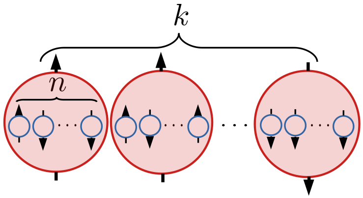
$\Lambda_{{\rm tr}_{N-k}}$ $\Lambda_{\textrm{BnS}}^{N\rightarrow k}$

(b)

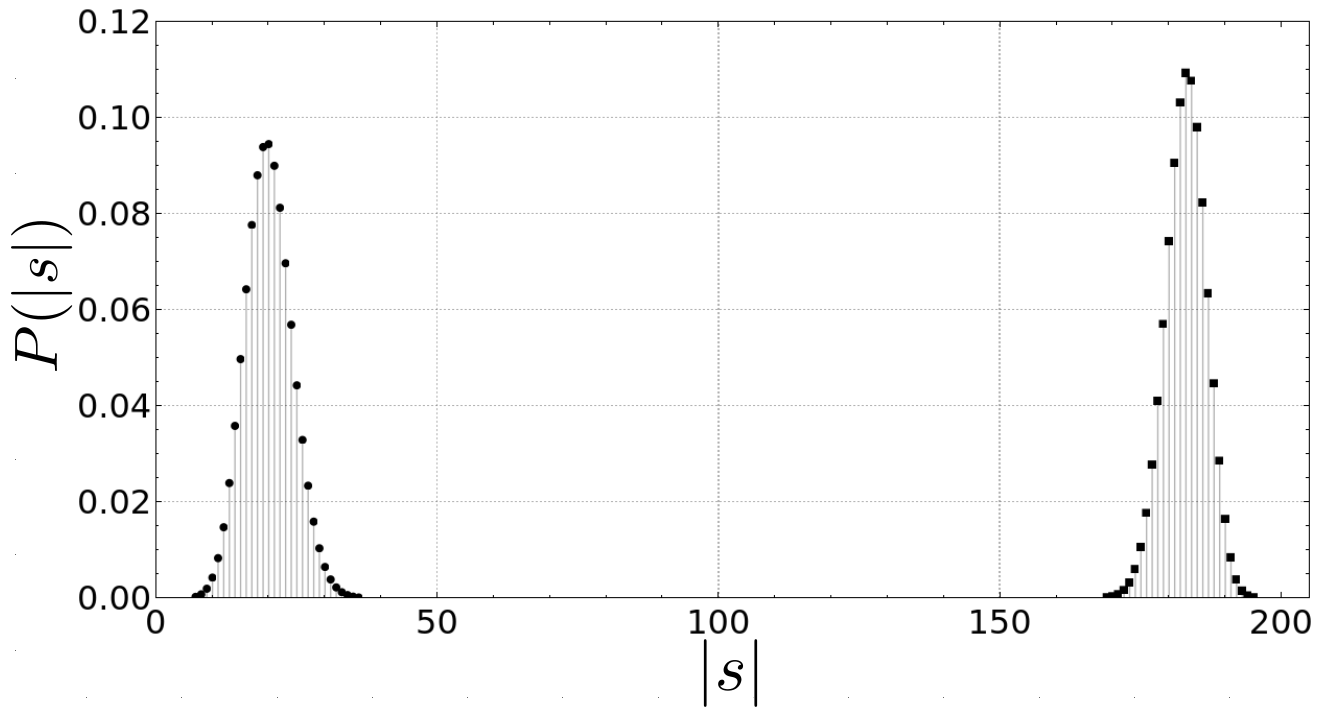
(c)

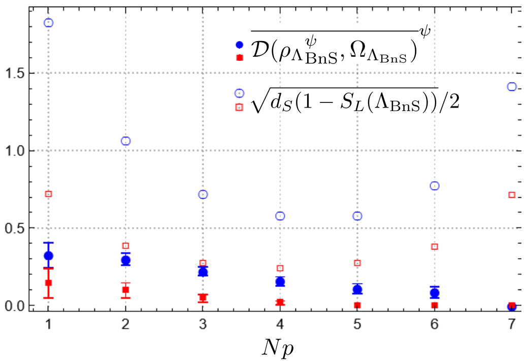
Figure 1: (a) Subsystems scenarios. On the left panel it is shown the usual link between particles and degrees-of-freedom. In this case, a subsystem is simply a subset of the constituent particles: from a system of $N$ spins, a subsystem of $k$ spins is obtained by tracing out $N-k$ spins, i.e., by applying the map $\Lambda_{{\rm tr}_{N-k}}$. On the right is an example of a generalized subsystem, which is suggested by a blurred and saturated fluorescence detection. In this case, blocks of $n$ spins give rise to one effective spin. The description of a effective subsystem of $k$ spins coming from an underlying system of $N$ spins is obtained by the action of the channel $\Lambda_{\textrm{BnS}}^{N\rightarrow k}$. (b) Canonical Distributions. Considering the Hamiltonian $H=-\hbar\omega\sum_{i=1}^{N}Z_{i}/2$ for both scenarios shown in (a), it is clear that the number of excited states $|s|$ is directly related to the energy of the system. In this panel we plot the probability distribution of $|s|$ for both cases: the points on the left (circles) represent the energy distribution for the partial trace case, while the points on the right (squares) are related to the blurred and saturated situation. For this plot we used $N=10000$, $Np=200$ and $k=1000$. (c) Canonical typicality for the blurred and saturated generalized subsystem. For this plot the filled markers represent the average distance to the generalized canonical state, and the hollow markers show the bound in Eq. (3). The underlying system here is composed by $N=8$ spins, with the red (squares) points representing the case where $k=2$ and the blue (circles) points the case $k=4$.

Conclusions. This work is a first step towards a statistical mechanics of generalized subsystems. We introduced the canonical state for generalized subsystems and showed that there are situations where it is drastically different from the canonical state one would obtain by associating the relevant degrees-of-freedom of a physical scenario with the particles that constitute the system. Moreover, we also showed that the phenomena of canonical typicality is also present for generalized subsystems, and thus all the foundational ingredients of traditional statistical mechanics are inherited by this new picture. Given our all-encompassing description of physical systems, it became explicit that the quantity which controls the emergence of canonical typicality is the entropy of the channel used to define the generalized subsystem.

One last remark is in order. In the formalism shown above we employed quantum channels exclusively to define the generalized subsystems. However, given the formalism’s flexibility, we could simply change $\Lambda$ by a composition of quantum channels as $\Lambda\circ\Gamma$, with $\Gamma:\mathcal{L}(\mathcal{H}_{R})\mapsto\mathcal{L}(\mathcal{H}_{R})$, without altering any of the presented results. In this situation $\Gamma$ can be thought as a pre-processing of the underlying description, with the pure states of $\mathcal{H}_{R}$ generically being mapped into mixed ones. Such a possibility is interesting in at least two ways. First it shows that the phenomena of canonical typicality is robust to noise, which might substantiate the success of ensembles. Second, this might alleviate the unreasonable requirement for canonical typicality that the underlying states whose effective description behave similarly to the canonical state, are states taken uniformly from the Haar measure. For complex systems we do not expect Nature to be able to efficiently produce such states [28], and thus this requirement puts in doubt the relevance of the typicality approach. By pre-processing the states from the Haar measure, we are effectively inducing a new measure, which might lead to more physically feasible samples. For instance, it is expected that the average amount of entanglement to drop after the pre-processing, possibly making the production of the output states a much easier task.

Altogether, the presented formalism not only will give a more suitable description of the statistical mechanics of highly isolated and strongly interacting complex systems, but it might also shed light on some conceptual issues of traditional statistical mechanics.

Acknowledgements. This work is supported in part by the National Council for Scientific and Technological Development, CNPq Brazil (projects: Universal Grant No. 406499/2021-7, and 409611/2022-0), and it is part of the Brazilian National Institute for Quantum Information. TRO acknowledges funding from the Air Force Office of Scientific Research under Grant No. FA9550-23-1-0092.

Appendix A Appendix A: Applying Levy’s Lemma to $\mathcal{D}({\varrho}_{\Lambda}^{\psi},\Omega_{\Lambda})$

Lemma (Levy’s Lemma): Given a Lipschitz continuous function $f:\mathbb{S}^{d}\rightarrow\mathbb{R}$, and a point $\psi\in\mathbb{S}^{d}$ chosen uniformly at random,

$${\rm Pr}_{\psi}\big{[}|f(\psi)-\overline{f}|\geq\epsilon\big{]}\leq 2\exp\bigg{(}\dfrac{-2G(d+1)\epsilon^{2}}{\eta^{2}}\bigg{)},$$ (8)

where $\eta$ is the Lipschitz constant of $f$ with respect to the Euclidean norm (see below), $G$ is a positive constant (which can be taken to be $G=(18\pi^{3})^{-1}$), and $\overline{f}$ is the mean value of $f$ over the uniform measure in $\mathbb{S}^{d}$.

After noticing that the space of pure quantum states in a $d$-dimensional Hilbert space ($\mathcal{H}_{d}$) can be described as a hyper-sphere embedded in a $2d$ real space, $\mathbb{S}^{2d-1}$, we can apply Levy’s Lemma to Lipschitz continuous properties of pure states by sampling them from the Haar measure.

In our case, we are interest in applying Levy’s Lemma to $f(\psi)=\mathcal{D}({\varrho}_{\Lambda}^{\psi},\Omega_{\Lambda})$ with $\psi\in\mathbb{S}^{2d_{R}-1}$. It remains to show that such a function is Lipschitz continuous with respect to the Euclidean norm.

Generally, a function $f:X\mapsto Y$ between metric spaces is Lipschitz continuous if there exists a constant $\eta\in\mathds{R}^{+}$ such that for all $a,b\in X$ we have $\delimiter 69645069f(a)-f(b)\delimiter 86422285_{Y}\leq\eta\delimiter 69645069a-b\delimiter 86422285_{X}$. Here $\delimiter 69645069\cdot\delimiter 86422285_{Z}$ is a norm associated with space $Z$. Lispschitz continuity is then a strong form of continuity.

For our case, we must upper bound $|\mathcal{D}({\varrho}_{\Lambda}^{\psi},\Omega_{\Lambda})-\mathcal{D}({\varrho}_{\Lambda}^{\phi},\Omega_{\Lambda})|$ for any $\psi$ and $\phi$ in $\mathbb{S}^{2d_{R}-1}$. It goes as follows [16]:

$$|\mathcal{D}({\varrho}_{\Lambda}^{\psi},\Omega_{\Lambda})-\mathcal{D}({\varrho}_{\Lambda}^{\phi},\Omega_{\Lambda})|^{2} =|\delimiter 69645069\Lambda(\psi)-\Lambda(\mathcal{E}_{R})\delimiter 86422285_{1}-\delimiter 69645069\Lambda(\phi)-\Lambda(\mathcal{E}_{R})\delimiter 86422285_{1}|^{2}/4;$$

$$\leq\delimiter 69645069\Lambda(\psi)-\Lambda(\phi)\delimiter 86422285_{1}^{2}/4;$$

$$\leq\eta_{\Lambda}^{2}\delimiter 69645069|\psi\rangle\!\langle\psi|-|\phi\rangle\!\langle\phi|\delimiter 86422285_{1}^{2}/4;$$

$$=\eta_{\Lambda}^{2}(1-|\langle\psi|\phi\rangle|^{2});$$

$$\leq\eta_{\Lambda}^{2}\delimiter 69645069\delimiter 69640972\psi\rangle-\delimiter 69640972\phi\rangle\delimiter 86422285^{2}.$$

This proves that $f(\psi)=\mathcal{D}({\varrho}_{\Lambda}^{\psi},\Omega_{\Lambda})$ is Lipschitz continuous with constant $\eta_{\Lambda}$.

We then obtain the desired result:

$${\rm Pr}_{\psi}\Big{[}\big{|}\mathcal{D}\left(\Lambda(|\psi\rangle\!\langle\psi|),\Omega_{\Lambda}\right)-\overline{\mathcal{D}({\varrho}_{\Lambda}^{\chi},\Omega_{\Lambda})}^{\chi}\big{|}\geq\epsilon\Big{]}\leq 2\textrm{e}^{-C\frac{d_{\text{R}}\epsilon^{2}}{\eta_{\Lambda}^{2}}}.$$ (9)

where $C$ is a constant that can be taken equal to $2/9\pi^{3}$, and $\eta_{\Lambda}$ is the channel Lipschitz constant.

Appendix B APPENDIX B: Full map $\Lambda:\mathbb{C}_{3}\mapsto\mathbb{C}_{2}$

For completeness, here we present the full map that singles out an effective 2-dimensional subsystem from a tree-level system whose excited level cannot be distinguished. The map action in a generic linear operator ${\varrho}=[{\varrho}]_{ij}$ with $i,j\in\{0,1,2\}$ is as follows:

$$\Lambda({\varrho})=\begin{pmatrix}{\varrho}_{00}&\frac{{\varrho}_{01}+{\varrho}_{02}}{\sqrt{2}}\\ \frac{{\varrho}_{10}+{\varrho}_{20}}{\sqrt{2}}&{\varrho}_{11}+{\varrho}_{22}\end{pmatrix}.$$ (10)

The isometry $V:\mathbb{C}_{3}\mapsto\mathbb{C}_{2}\otimes\mathbb{C}_{2}$ defining this channel is given by:

$$V=\begin{pmatrix}1&0&0\\ 0&0&0\\ 0&\frac{1}{\sqrt{2}}&\frac{1}{\sqrt{2}}\\ 0&\frac{1}{\sqrt{2}}&-\frac{1}{\sqrt{2}}\end{pmatrix}.$$ (11)

Appendix C APPENDIX C: PROVING $\mathcal{D}({\varrho}_{\Lambda}^{\psi},\Omega_{\Lambda})\leq\frac{1}{2}\sqrt{d_{B}(1-S_{L}(\Lambda))}$

Given that the definitions of the trace-norm $\parallel A\parallel_{1}={\rm tr}\big{[}\sqrt{A^{\dagger}A}\big{]}$ and Hilbert-Schmidt norm $\parallel A\parallel_{2}=\sqrt{{\rm tr}[A^{\dagger}A]}$. For any $n\times n$ matrix $A$ the following inequality is satisfied:

$$\parallel A\parallel_{1}\leq\sqrt{n}\parallel A\parallel_{2}.$$ (12)

This relation can be easily proved, considering that $A$ has eigenvalues $\lambda_{i}$, and the convexity of the square function:

$$\parallel A\parallel_{1}^{2}=n^{2}\bigg{(}\dfrac{1}{n}\sum_{i}|\lambda_{i}|\bigg{)}^{2}\leq n^{2}\dfrac{1}{n}\sum_{i}|\lambda_{i}|^{2}=n\parallel A\parallel_{2}^{2}.$$

Let us derive another useful relation. Doing $A={\varrho}_{\Lambda}^{\psi}-\Omega_{\Lambda}$ and taking the average in the Hilbert-Schmidt norm:

$$\overline{\parallel{\varrho}_{\Lambda}^{\psi}-\Omega_{\Lambda}\parallel_{2}}^{\psi} \leq\sqrt{\overline{\parallel{\varrho}_{\Lambda}^{\psi}-\Omega_{\Lambda}\parallel_{2}^{2}}^{\psi}}$$

$$=\sqrt{\overline{{\rm tr}[({\varrho}_{\Lambda}^{\psi}-\Omega_{\Lambda})^{2}]}^{\psi}}=\sqrt{\overline{{\rm tr}[({\varrho}_{\Lambda}^{\psi})^{2}]}^{\psi}-2\overline{{\rm tr}[{\varrho}_{\Lambda}^{\psi}\Omega_{\Lambda}]}^{\psi}+\overline{{\rm tr}[\Omega_{\Lambda}^{2}]}^{\psi}}=\sqrt{\overline{{\rm tr}[({\varrho}_{\Lambda}^{\psi})^{2}]}^{\psi}-2{\rm tr}[\overline{{\varrho}_{\Lambda}^{\psi}}^{\psi}\Omega_{\Lambda}]+{\rm tr}[\Omega_{\Lambda}^{2}]}$$

$$=\sqrt{\overline{{\rm tr}[({\varrho}_{\Lambda}^{\psi})^{2}]}^{\psi}-{\rm tr}[\Omega_{\Lambda}^{2}]},$$ (13)

in the first line we used the Jensen’s inequality $f(\overline{M})\leq\overline{f(M)}$ with $f(\cdot)=(\cdot)^{2}$. In the third line we used $\overline{\Omega_{\Lambda}}^{\psi}=\overline{{\varrho}_{\Lambda}^{\psi}}^{\psi}=\Omega_{\Lambda}$.

Then, from (12) and (13):

$$\overline{\mathcal{D}({\varrho}_{\Lambda}^{\psi},\Omega_{\Lambda})}^{\psi}=\dfrac{1}{2}\overline{\parallel{\varrho}_{\Lambda}^{\psi}-\Omega_{\Lambda}\parallel_{1}}^{\psi}\leq\dfrac{1}{2}\sqrt{d_{B}\big{(}\overline{{\rm tr}[({\varrho}_{\Lambda}^{\psi})^{2}]}^{\psi}-{\rm tr}[\Omega_{\Lambda}^{2}]\big{)}}$$ (14)

C.1 Calculating $\overline{{\rm tr}[({\varrho}_{\Lambda}^{\psi})^{2}]}^{\psi}$

To calculate $\overline{{\rm tr}[({\varrho}_{\Lambda}^{\psi})^{2}]}^{\psi}$, it is helpful to duplicate the original Hilbert space, extending the problem from $\mathcal{H}_{R}$ to $\mathcal{H}_{R}\otimes\mathcal{H}_{R^{\prime}}$. We start by written ${\rm tr}[({\varrho}_{\Lambda}^{\psi})^{2}]$ as:

$${\rm tr}[({\varrho}_{\Lambda}^{\psi})^{2}] =\sum_{i}({\varrho}_{ii})^{2}$$

$$=\sum_{i,j,i^{\prime},j^{\prime}}({\varrho}_{ij})({\varrho}_{i^{\prime}j^{\prime}})\langle ii^{\prime}|jj^{\prime}\rangle\langle i^{\prime}i|jj^{\prime}\rangle$$

$$={\rm tr}_{SS^{\prime}}[({\varrho}_{\Lambda}^{\psi}\otimes{\varrho}_{\Lambda^{\prime}}^{\psi})F_{SS^{\prime}}],$$ (15)

where the $F_{SS^{\prime}}$ is the swap operation $S\leftrightarrow S^{\prime}$:

$$F_{SS^{\prime}}=\sum_{ss^{\prime}}\delimiter 69640972s^{\prime}\rangle\langle s\delimiter 86418188\otimes\delimiter 69640972s\rangle\langle s^{\prime}\delimiter 86418188$$ (16)

and then

$$\overline{{\rm tr}[({\varrho}_{\Lambda}^{\psi})^{2}]}^{\psi} =\overline{{\rm tr}_{SS^{\prime}}[({\varrho}_{\Lambda}^{\psi}\otimes{\varrho}_{\Lambda^{\prime}}^{\psi})F_{SS^{\prime}}]}^{\psi}$$

$$=\overline{{\rm tr}_{SS^{\prime}}[(\Lambda[\delimiter 69640972\psi\rangle\langle\psi\delimiter 86418188]\otimes\Lambda[\delimiter 69640972\psi\rangle\langle\psi\delimiter 86418188])F_{SS^{\prime}}]}^{\psi}$$

$$=\overline{{\rm tr}_{SS^{\prime}}[(\Lambda\otimes\Lambda)[\delimiter 69640972\psi\rangle\langle\psi\delimiter 86418188\otimes\delimiter 69640972\psi\rangle\langle\psi\delimiter 86418188]F_{SS^{\prime}}]}^{\psi}$$

$$={\rm tr}_{SS^{\prime}}[(\Lambda\otimes\Lambda)[\overline{\delimiter 69640972\psi\rangle\langle\psi\delimiter 86418188\otimes\delimiter 69640972\psi\rangle\langle\psi\delimiter 86418188}^{\psi}]F_{SS^{\prime}}]$$ (17)

Using the result [bibid]

$$\overline{\delimiter 69640972\psi\rangle\langle\psi\delimiter 86418188\otimes\delimiter 69640972\psi\rangle\langle\psi\delimiter 86418188}^{\psi}=\dfrac{\mathds{1}_{RR^{\prime}}+F_{RR^{\prime}}}{d_{R}(d_{R}+1)}$$ (18)

where $\mathds{1}_{RR^{\prime}}=\mathds{1}_{R}\otimes\mathds{1}_{R^{\prime}}$. Using above equation in (17):

$$\overline{{\rm tr}[({\varrho}_{\Lambda}^{\psi})^{2}]}^{\psi} ={\rm tr}_{SS^{\prime}}\big{[}(\Lambda\otimes\Lambda)\big{[}\dfrac{\mathds{1}_{RR^{\prime}}}{d_{R}(d_{R}+1)}\big{]}F_{SS^{\prime}}\big{]}+{\rm tr}_{SS^{\prime}}\big{[}(\Lambda\otimes\Lambda)\big{[}\dfrac{\mathds{F}_{RR^{\prime}}}{d_{R}(d_{R}+1)}\big{]}F_{SS^{\prime}}\big{]}$$

$$\leq{\rm tr}_{S}[\Omega_{\Lambda}^{2}]+{\rm tr}_{SS^{\prime}}\big{[}(\Lambda\otimes\Lambda)\big{[}\dfrac{F_{RR^{\prime}}}{d_{R}^{2}}\big{]}F_{SS^{\prime}}\big{]}$$ (19)

in the last line we used $d_{R}(d_{R}+1)\geq d_{R}^{2}$.

Thus, (19) in (14):

$$\overline{\parallel{\varrho}_{\Lambda}^{\psi}-\Omega_{\Lambda}\parallel_{1}}^{\psi}\leq\sqrt{\dfrac{d_{S}}{d_{R}^{2}}\;{\rm tr}_{SS^{\prime}}[(\Lambda\otimes\Lambda)[F_{RR^{\prime}}]F_{SS^{\prime}}]}.$$ (20)

Using (16) in ${\rm tr}_{SS^{\prime}}[(\Lambda\otimes\Lambda)[F_{RR^{\prime}}]F_{SS^{\prime}}]$:

$${\rm tr}_{SS^{\prime}}[(\Lambda\otimes\Lambda)[F_{RR^{\prime}}]F_{SS^{\prime}}] ={\rm tr}_{SS^{\prime}}\big{[}(\Lambda\otimes\Lambda)\big{[}\sum_{r,r^{\prime}=0}^{d_{R}-1}\delimiter 69640972r^{\prime}\rangle\langle r\delimiter 86418188\otimes\delimiter 69640972r\rangle\langle r^{\prime}\delimiter 86418188\big{]}F_{SS^{\prime}}\big{]}$$

$$={\rm tr}_{SS^{\prime}}\big{[}\big{(}\sum_{r,r^{\prime}=0}^{d_{R}-1}\Lambda\big{[}\delimiter 69640972r^{\prime}\rangle\langle r\delimiter 86418188\big{]}\otimes\Lambda\big{[}\delimiter 69640972r\rangle\langle r^{\prime}\delimiter 86418188\big{]}\big{)}F_{SS^{\prime}}\big{]}$$ (21)

using the Kraus representation (22) of $\Lambda$. Any quantum channel $\Lambda:\mathcal{L}(\mathcal{H}_{R})\rightarrow\mathcal{L}(\mathcal{H}_{S})$, there exist a representation

$$\Lambda[\psi]=\sum_{m=1}^{\tau}K_{m}\psi K_{m}^{\dagger}$$ (22)

for all $\psi\in\mathcal{L}(\mathcal{H}_{R})$, $K_{m}\in\mathcal{L}(\mathcal{H}_{R},\mathcal{H}_{S})$ for all $m\in\{1,\dots,\tau\}$ and $\tau$ need not be any larger than $d_{R}d_{S}$. The expression (22) is a Kraus representation of the map $\Lambda$, unlike the Choi representation, Kraus representations are not unique.

Using (16) and (22) in (21)

$${\rm tr}_{SS^{\prime}}[(\Lambda\otimes\Lambda)[F_{RR^{\prime}}]F_{SS^{\prime}}] ={\rm tr}_{SS^{\prime}}\big{[}\big{(}\sum_{r,r^{\prime}=0}^{d_{R}-1}\sum_{m,n=1}^{\tau}K_{m}\delimiter 69640972r^{\prime}\rangle\langle r\delimiter 86418188K_{m}^{\dagger}\otimes K_{n}\delimiter 69640972r\rangle\langle r^{\prime}\delimiter 86418188K_{n}^{\dagger}\big{)}\sum_{s,s^{\prime}=0}^{d_{S}-1}\delimiter 69640972s^{\prime}\rangle\langle s\delimiter 86418188\otimes\delimiter 69640972s\rangle\langle s^{\prime}\delimiter 86418188\big{]}$$

$$={\rm tr}_{SS^{\prime}}\big{[}\sum_{r,r^{\prime}=0}^{d_{R}-1}\sum_{m,n=1}^{\tau}\sum_{s,s^{\prime}=0}^{d_{S}-1}K_{m}\delimiter 69640972r^{\prime}\rangle\langle r\delimiter 86418188K_{m}^{\dagger}\delimiter 69640972s^{\prime}\rangle\langle s\delimiter 86418188\otimes K_{n}\delimiter 69640972r\rangle\langle r^{\prime}\delimiter 86418188K_{n}^{\dagger}\delimiter 69640972s\rangle\langle s^{\prime}\delimiter 86418188\big{]}$$

$$=\sum_{t,t^{\prime}=0}^{d_{S}-1}\sum_{r,r^{\prime}=0}^{d_{R}-1}\sum_{m,n=1}^{\tau}\sum_{s,s^{\prime}=0}^{d_{S}-1}\langle t\delimiter 86418188K_{m}\delimiter 69640972r^{\prime}\rangle\langle r\delimiter 86418188K_{m}^{\dagger}\delimiter 69640972s^{\prime}\rangle\overbrace{\langle s\delimiter 86418188t}^{\delta_{st}}\rangle\langle t^{\prime}\delimiter 86418188K_{n}\mathds{1}_{R^{\prime}}\delimiter 69640972r\rangle\langle r^{\prime}\delimiter 86418188K_{n}^{\dagger}\delimiter 69640972s\rangle\overbrace{\langle s^{\prime}\delimiter 86418188t^{\prime}}^{\delta_{s^{\prime}t^{\prime}}}\rangle$$

$$=\sum_{r,r^{\prime}=0}^{d_{R}-1}\sum_{m,n=1}^{\tau}\sum_{s,s^{\prime}=0}^{d_{S}-1}\langle s\delimiter 86418188K_{m}\delimiter 69640972r^{\prime}\rangle\langle r\delimiter 86418188K_{m}^{\dagger}\delimiter 69640972s^{\prime}\rangle\langle s^{\prime}\delimiter 86418188K_{n}\delimiter 69640972r\rangle\langle r^{\prime}\delimiter 86418188K_{n}^{\dagger}\delimiter 69640972s\rangle$$

$$=\sum_{m,n=1}^{\tau}\sum_{s,s^{\prime}=0}^{d_{S}-1}\langle s\delimiter 86418188K_{m}\underbrace{\big{(}\sum_{r^{\prime}=0}^{d_{R}-1}\delimiter 69640972r^{\prime}\rangle\langle r^{\prime}\delimiter 86418188\big{)}}_{=\mathds{1}_{R}}K_{n}^{\dagger}\delimiter 69640972s\rangle\langle s^{\prime}\delimiter 86418188K_{n}\underbrace{\big{(}\sum_{r=0}^{d_{R}-1}\delimiter 69640972r\rangle\langle r\delimiter 86418188\big{)}}_{=\mathds{1}_{R}}K_{m}^{\dagger}\delimiter 69640972s^{\prime}\rangle$$

$$=\sum_{m,n=1}^{\tau}\sum_{s,s^{\prime}=0}^{d_{S}-1}\langle s\delimiter 86418188K_{m}K_{n}^{\dagger}\delimiter 69640972s\rangle\langle s^{\prime}\delimiter 86418188K_{n}K_{m}^{\dagger}\delimiter 69640972s^{\prime}\rangle$$

$$=\sum_{m,n=1}^{\tau}{\rm tr}[K_{m}K_{n}^{\dagger}]{\rm tr}[K_{n}K_{m}^{\dagger}]=\sum_{m,n=1}^{\tau}|{\rm tr}[K_{m}K_{n}^{\dagger}]|^{2}$$ (23)

above result in (20), we have:

$$\mathcal{D}({\varrho}_{\Lambda}^{\psi},\Omega_{\Lambda})\leq\dfrac{1}{2}\sqrt{\dfrac{d_{S}}{d_{R}^{2}}\sum_{m,n=i}^{\tau}\big{|}{\rm tr}\big{[}K_{m}K_{n}^{\dagger}\big{]}\big{|}^{2}}.$$ (24)

Rewriting the above equation in terms of Choi-Jamiołkowski state, $J_{\Lambda}:=\Lambda\otimes\mathds{1}(|\phi^{+}\rangle\!\langle\phi^{+}|)$ of the quantum channel $\Lambda$, where $\delimiter 69640972\phi^{+}\rangle=\sum_{i}\delimiter 69640972ii\rangle/\sqrt{d_{R}}\in\mathcal{H}_{R}\otimes\mathcal{H}_{R}$. Using the Krauss form:

$$J_{\Lambda} =(\Lambda\otimes\mathds{1}_{R})[\delimiter 69640972\phi_{+}\rangle\langle\phi_{+}\delimiter 86418188]$$

$$=\dfrac{1}{d_{R}}\sum_{i,j=0}^{d_{R}-1}\Lambda[\delimiter 69640972i\rangle\langle j\delimiter 86418188]\otimes\delimiter 69640972i\rangle\langle j\delimiter 86418188=\dfrac{1}{d_{R}}\sum_{i,j=0}^{d_{R}-1}\sum_{m=1}^{\tau}K_{m}\delimiter 69640972i\rangle\langle j\delimiter 86418188K_{m}^{\dagger}\otimes\delimiter 69640972i\rangle\langle j\delimiter 86418188$$ (25)

Calculating ${d_{R}}^{2}{\rm tr}[{J_{\Lambda}}^{2}]$:

$${d_{R}}^{2}{\rm tr}[{J_{\Lambda}}^{2}] ={\rm tr}_{SR}\bigg{[}\big{(}\sum_{i,j=0}^{d_{R}-1}\sum_{m=1}^{\tau}K_{m}\delimiter 69640972i\rangle\langle j\delimiter 86418188K_{m}^{\dagger}\otimes\delimiter 69640972i\rangle\langle j\delimiter 86418188\big{)}\big{(}\sum_{i^{\prime},j^{\prime}=0}^{d_{R}-1}\sum_{n=1}^{\tau}K_{n}\delimiter 69640972i^{\prime}\rangle\langle j^{\prime}\delimiter 86418188K_{n}^{\dagger}\otimes\delimiter 69640972i^{\prime}\rangle\langle j^{\prime}\delimiter 86418188\big{)}\bigg{]}$$

$$={\rm tr}_{SR}\bigg{[}\sum_{i,j,i^{\prime},j^{\prime}}\sum_{m,n}K_{m}\delimiter 69640972i\rangle\langle j\delimiter 86418188K_{m}^{\dagger}K_{n}\delimiter 69640972i^{\prime}\rangle\langle j^{\prime}\delimiter 86418188K_{n}^{\dagger}\otimes\delimiter 69640972i\rangle\overbrace{\langle j\delimiter 86418188i^{\prime}\rangle}^{\delta_{ji^{\prime}}}\langle j^{\prime}\delimiter 86418188\bigg{]}$$

$$={\rm tr}_{SR}\bigg{[}\sum_{i,j,j^{\prime}}\sum_{m,n}K_{m}\delimiter 69640972i\rangle\langle j\delimiter 86418188K_{m}^{\dagger}K_{n}\delimiter 69640972j\rangle\langle j^{\prime}\delimiter 86418188K_{n}^{\dagger}\otimes\delimiter 69640972i\rangle\langle j^{\prime}\delimiter 86418188\bigg{]}$$

$$=\sum_{s=0}^{d_{S}-1}\sum_{i,j,j^{\prime}}\sum_{m,n}\langle s\delimiter 86418188K_{m}\delimiter 69640972i\rangle\langle j\delimiter 86418188K_{m}^{\dagger}K_{n}\delimiter 69640972j\rangle\langle j^{\prime}\delimiter 86418188K_{n}^{\dagger}\delimiter 69640972s\rangle\overbrace{\sum_{r=0}^{d_{R}-1}\langle r\delimiter 69640972i\rangle\langle j^{\prime}\delimiter 86418188r\rangle}^{\delta_{j^{\prime}i}}$$

$$=\sum_{s}\sum_{i,j}\sum_{m,n}\langle s\delimiter 86418188K_{m}\delimiter 69640972i\rangle\langle j\delimiter 86418188K_{m}^{\dagger}K_{n}\delimiter 69640972j\rangle\langle i\delimiter 86418188K_{n}^{\dagger}\delimiter 69640972s\rangle$$

$$=\sum_{s}\sum_{j}\sum_{m,n}\langle s\delimiter 86418188K_{m}\bigg{(}\sum_{i}\delimiter 69640972i\rangle\langle i\delimiter 86418188\bigg{)}K_{n}^{\dagger}\delimiter 69640972s\rangle\langle j\delimiter 86418188K_{m}^{\dagger}K_{n}\delimiter 69640972j\rangle$$

$$=\sum_{s}\sum_{j}\sum_{m,n}\langle s\delimiter 86418188K_{m}K_{n}^{\dagger}\delimiter 69640972s\rangle\langle j\delimiter 86418188K_{m}^{\dagger}K_{n}\delimiter 69640972j\rangle$$

$$=\sum_{m,n}\bigg{(}\sum_{s}\langle s\delimiter 86418188K_{m}K_{n}^{\dagger}\delimiter 69640972s\rangle\bigg{)}\bigg{(}\sum_{j}\langle j\delimiter 86418188K_{m}^{\dagger}K_{n}\delimiter 69640972j\rangle\bigg{)}$$

$$=\sum_{m,n}{\rm tr}\big{[}K_{m}K_{n}^{\dagger}\big{]}\overbrace{{\rm tr}\big{[}K_{m}^{\dagger}K_{n}\big{]}}^{{\rm tr}\big{[}K_{n}K_{m}^{\dagger}\big{]}}=\sum_{m,n=1}^{\tau}|{\rm tr}[K_{m}K_{n}^{\dagger}]|^{2}$$ (26)

So (24) can be written in terms of the purity of the Choi-Jamiołkowski state

$$\mathcal{D}({\varrho}_{\Lambda}^{\psi},\Omega_{\Lambda})\leq\dfrac{1}{2}\sqrt{d_{S}{\rm tr}\big{[}{J_{\Lambda}}^{2}\big{]}},$$ (27)

or in terms of the linear entropy of the map:

$$\mathcal{D}({\varrho}_{\Lambda}^{\psi},\Omega_{\Lambda})\leq\dfrac{1}{2}\sqrt{d_{S}(1-S_{L}(\Lambda))}.,$$ (28)

since $S_{L}(\Lambda)=1-{\rm tr}\big{[}{J_{\Lambda}}^{2}\big{]}$.

Appendix D Appendix D: Demonstrating that $\sqrt{d_{S}{\rm tr}(J_{{\rm tr}_{E}}^{2})}=\sqrt{\frac{d_{S}}{d_{E}^{eff}}}$

This section aims to demonstrate that (1) is a particular case of (3) when $\Lambda={\rm tr}_{E}$. So we need to show that ${\rm tr}(J_{{\rm tr}_{E}}^{2})=1/{d_{E}^{\text{eff}}}$.

The partial trace act on the entire global space ${\rm tr}_{E}:\mathcal{L}(\mathcal{H}_{S}\otimes\mathcal{H}_{E})\rightarrow\mathcal{L}(\mathcal{H}_{S})$ and ${\rm tr}_{S}:\mathcal{L}(\mathcal{H}_{S}\otimes\mathcal{H}_{E})\rightarrow\mathcal{L}(\mathcal{H}_{E})$. However, note that the microcanonical state $\mathds{1}_{R}/d_{R}$ is defined in the restricted space $\mathcal{H}_{R}\subseteq\mathcal{H}_{S}\otimes\mathcal{H}_{E}$, so it is convenient we choose a basis $\{\delimiter 69640972R_{r}\rangle\}\in\mathcal{H}_{R}$ in which elements can be written as:

$$\delimiter 69640972R_{r}\rangle=\sum_{ij}c^{r}_{ij}\delimiter 69640972i\rangle\otimes\delimiter 69640972j\rangle$$ (29)

with $\delimiter 69640972i\rangle$ and $\delimiter 69640972j\rangle$ orthonormal basis for $\mathcal{H}_{S}$ and $\mathcal{H}_{E}$, respectively.

In order to find the Choi state, let us first consider the maximally entangles state $\delimiter 69640972phi_{+}\rangle\in\mathcal{H}_{R}\otimes\mathcal{H}_{R}$, in which its density matrix can be conveniently written as:

$$\delimiter 69640972\phi_{+}\rangle\langle\phi_{+}\delimiter 86418188 =\dfrac{1}{d_{R}}\sum_{r,t}\delimiter 69640972R_{r}\rangle\langle R_{t}\delimiter 86418188\otimes\delimiter 69640972R_{r}\rangle\langle R_{t}\delimiter 86418188$$

$$=\dfrac{1}{d_{R}}\sum_{r,t}\left(\sum_{i,j,k,l}c^{r}_{ij}c^{t\ast}_{k,l}\delimiter 69640972ij\rangle\langle kl\delimiter 86418188\right)\otimes\delimiter 69640972R_{r}\rangle\langle R_{t}\delimiter 86418188$$

So the Choi state related to the map ${\rm tr}_{E}$ is given by

$$J_{{\rm tr}_{E}} =({\rm tr}_{E}\otimes\mathds{1}_{R})(\delimiter 69640972\phi_{+}\rangle\langle\phi_{+}\delimiter 86418188)=\dfrac{1}{d_{R}}\sum_{r,t}\left(\sum_{i,j,k,l}c^{r}_{ij}c^{t\ast}_{k,l}{\rm tr}_{E}(\delimiter 69640972ij\rangle\langle kl\delimiter 86418188)\right)\otimes\delimiter 69640972R_{r}\rangle\langle R_{t}\delimiter 86418188$$

$$=\dfrac{1}{d_{R}}\sum_{i,k,r,t}\left(\sum_{j}c^{r}_{ij}c^{t\ast}_{k,j}\right)\delimiter 69640972i\rangle\langle k\delimiter 86418188\otimes\delimiter 69640972R_{r}\rangle\langle R_{t}\delimiter 86418188$$ (31)

Calculating the purity

$${\rm tr}(J_{{\rm tr}_{E}}^{2}) ={\rm tr}\left[\dfrac{1}{d_{R}^{2}}\sum_{i,k,r,t,m,n,p,q}\left(\left(\sum_{j}c^{r}_{ij}c^{t\ast}_{kj}\right)\delimiter 69640972i\rangle\langle k\delimiter 86418188\otimes\delimiter 69640972R_{r}\rangle\langle R_{t}\delimiter 86418188\right)\left(\left(\sum_{z}c^{p}_{mz}c^{q\ast}_{nz}\right)\delimiter 69640972m\rangle\langle n\delimiter 86418188\otimes\delimiter 69640972R_{p}\rangle\langle R_{q}\delimiter 86418188\right)\right]$$

$$=\dfrac{1}{d_{R}^{2}}\sum_{i,k,r,t,m,n,p,q}\left(\sum_{j}c^{r}_{ij}c^{t\ast}_{kj}\right)\left(\sum_{z}c^{p}_{mz}c^{q\ast}_{nz}\right)\delta_{km}\delta_{tp}\delta_{in}\delta_{rq}$$

$$=\dfrac{1}{d_{R}^{2}}\sum_{j,z}\left(\sum_{j}c^{r}_{ij}c^{t\ast}_{kj}\right)\left(\sum_{z}c^{t}_{kz}c^{r\ast}_{iz}\right)=\dfrac{1}{d_{R}^{2}}\sum_{j,z}\left(\sum_{r,i}c^{r}_{ij}c^{r\ast}_{iz}\right)\left(\sum_{t,k}c^{t}_{kz}c^{t\ast}_{kj}\right)$$ (32)

Since we want to prove ${\rm tr}(J_{{\rm tr}_{E}}^{2})=1/d_{E}^{\text{eff}}$ and the effective dimension of the environment is defined as $d_{E}^{\text{eff}}={\rm tr}(\Omega_{{\rm tr}_{S}}^{2})$, let us explicitly describe the state $\Omega_{{\rm tr}_{S}}$:

$$\Omega_{{\rm tr}_{S}}= {\rm tr}_{S}\left(\dfrac{\mathds{1}_{R}}{d_{R}}\right)=\dfrac{1}{d_{R}}{\rm tr}_{S}\left(\sum_{r}\delimiter 69640972R_{r}\rangle\langle R_{r}\delimiter 86418188\right)$$

$$=\dfrac{1}{d_{R}}{\rm tr}_{S}\left(\sum_{r}\sum_{i,j,k,l}c^{r}_{ij}c^{r\ast}_{kl}\delimiter 69640972ij\rangle\langle kl\delimiter 86418188\right)$$

$$=\dfrac{1}{d_{R}}\sum_{j,l}\left(\sum_{r,i}c^{r}_{ij}c^{r\ast}_{il}\right)\delimiter 69640972j\rangle\langle l\delimiter 86418188$$ (33)

Now, lt us calculate the purity,

$${\rm tr}\left(\Omega_{{\rm tr}_{S}}^{2}\right) ={\rm tr}\left[\dfrac{1}{d_{R}^{2}}\sum_{j,l,m,n}\left(\left(\sum_{r,i}c^{r}_{ij}c^{r\ast}_{il}\right)\delimiter 69640972j\rangle\langle l\delimiter 86418188\right)\left(\left(\sum_{t,k}c^{t}_{km}c^{t\ast}_{kn}\right)\delimiter 69640972m\rangle\langle n\delimiter 86418188\right)\right]$$

$$=\dfrac{1}{d_{R}^{2}}\sum_{j,l,m,n}\left(\sum_{r,i}c^{r}_{ij}c^{r\ast}_{il}\right)\left(\sum_{t,k}c^{t}_{km}c^{t\ast}_{kn}\right)\delta_{l,m}\delta_{j,n}$$

$$=\dfrac{1}{d_{R}^{2}}\sum_{j,l}\left(\sum_{r,i}c^{r}_{ij}c^{r\ast}_{il}\right)\left(\sum_{t,k}c^{t}_{kl}c^{t\ast}_{kj}\right)$$ (34)

We can easily check that above equation is equal to (32) if we change the indices labels $l\rightarrow z$, so we finish the demonstration.

Appendix E Appendix E: Blurred and Saturated channel $\Lambda_{\text{BnS}}^{n\rightarrow 1}$ and derivation of $\Omega_{\Lambda}^{\Lambda_{\text{BnS}}^{N\rightarrow k}}$

Considering that we split the $N$ atoms of the total system into $k=\frac{N}{n}$ blocks of $n$ atoms, the effective system will be equivalent to $k$ two-level atoms. Our starting point is the expression

$$\Omega_{\Lambda_{\textrm{BnS}}}=\frac{1}{{N\choose Np}}\sum_{s\in\{0,1\}^{k}:|s|\in\{\lceil kp\rceil,...,\min(Np,k)\}}\sum_{n_{1}+n_{2}+...+n_{|s|}=Np-|s|}{\frac{N}{k}\choose n_{1}+1}{\frac{N}{k}\choose n_{2}+1}...{\frac{N}{k}\choose n_{|s|}+1}|s\rangle\!\langle s|.$$ (35)

In the expression above, $|s|$ is the number of 1’s in the string $s$ and $n_{i}<\frac{N}{k}$, $\forall i\in[\,|s|\,]$. Simpliflying the second summations,

$$S=\sum_{n_{1}+n_{2}+...n_{|s|}=Np-|s|}{\frac{N}{k}\choose n_{1}+1}{\frac{N}{k}\choose n_{2}+1}...{\frac{N}{k}\choose n_{|s|}+1},$$ (36)

with $n_{i}<\frac{N}{k}$. Therefore, $n_{i}\leqslant\frac{N}{k}-1$ and

$$S=\sum_{n_{1}=0}^{\frac{N}{k}-1}\sum_{n_{2}=0}^{\frac{N}{k}-1}...\sum_{n_{|s|}=0}^{\frac{N}{k}-1}{\frac{N}{k}\choose n_{1}+1}{\frac{N}{k}\choose n_{2}+1}...{\frac{N}{k}\choose n_{|s|}+1}\delta(n_{1}+n_{2}+...+n_{|s|}-(Np-|s|)).$$ (37)

Noticing that

$$\delta(n_{1}+n_{2}+...+n_{|s|}-(Np-|s|))=\frac{1}{2\pi}\int_{0}^{2\pi}d\theta\,\,e^{i\theta n_{1}+n_{2}+...+n_{|s|}-Np-|s|},$$ (38)

$$S=\frac{1}{2\pi}\int_{0}^{2\pi}d\theta\,\,e^{-i\theta(Np-|s|)}\bigg{(}\sum_{n=0}^{\frac{N}{k}-1}{\frac{N}{k}\choose n+1}e^{i\theta n}\bigg{)}^{|s|}.$$ (39)

Making $m=n+1$,

$$\begin{split}S&=\frac{1}{2\pi}\int_{0}^{2\pi}d\theta\,\,e^{-i\theta(Np-|s|)}\bigg{(}\sum_{m=1}^{\frac{N}{k}}{\frac{N}{k}\choose m}e^{i\theta(m-1)}\bigg{)}^{|s|}\\ &=\frac{1}{2\pi}\int_{0}^{2\pi}d\theta\,\,e^{-i\theta(Np-|s|)}\bigg{(}\sum_{m=0}^{\frac{N}{k}}{\frac{N}{k}\choose m}e^{i\theta(m-1)}-e^{-i\theta}\bigg{)}^{|s|}\\ &=\frac{1}{2\pi}\int_{0}^{2\pi}d\theta\,\,e^{-i\theta Np}\bigg{(}\sum_{m=0}^{\frac{N}{k}}{\frac{N}{k}\choose m}e^{i\theta m}-1\bigg{)}^{|s|}.\\ \Rightarrow S&=\frac{1}{2\pi}\int_{0}^{2\pi}d\theta\,\,e^{-i\theta Np}\sum_{q=0}^{|s|}{|s|\choose q}\bigg{[}\sum_{m=0}^{\frac{N}{k}}{\frac{N}{k}\choose m}e^{i\theta m}\bigg{]}^{q}(-1)^{|s|-q}.\end{split}$$ (40)

Therefore,

$$\begin{split}S&=\sum_{q=0}^{|s|}{|s|\choose q}(-1)^{|s|-q}\frac{1}{2\pi}\int_{0}^{2\pi}d\theta e^{-i\theta Np}\sum_{m_{1}=0}^{\frac{N}{k}}{\frac{N}{k}\choose m_{1}}e^{i\theta m_{1}}...\sum_{m_{q}=0}^{\frac{N}{k}}{\frac{N}{k}\choose m_{q}}e^{i\theta m+q}\\ &=\sum_{q=0}^{|s|}{|s|\choose q}(-1)^{|s|-q}\sum_{m_{1}=0}^{\frac{N}{k}}\sum_{m_{2}=0}^{\frac{N}{k}}...\sum_{m_{q}=0}^{\frac{N}{k}}{\frac{N}{k}\choose m_{1}}{\frac{N}{k}\choose m_{2}}...{\frac{N}{k}\choose m_{q}}\delta(m_{1}+m_{2}+...+m_{q}-Np)\\ &=\sum_{q=0}^{|s|}{|s|\choose q}(-1)^{|s|-q}\sum_{m_{1}+m_{2}+...+m_{q}=Np}{\frac{N}{k}\choose m_{1}}{\frac{N}{k}\choose m_{2}}...{\frac{N}{k}\choose m_{q}}\\ \Rightarrow S&=\sum_{q=0}^{|s|}{|s|\choose q}(-1)^{|s|-q}{\frac{Nq}{k}\choose Np}.\end{split}$$ (41)

The canonical state is given by

$$\Omega_{\Lambda_{\textrm{BnS}}}=\frac{1}{d_{R}}\sum_{s\in\{0,1\}^{k}:|s|\in\{\lceil kp\rceil,...,\min(Np,k)\}}\sum_{q=0}^{|s|}{|s|\choose q}{\frac{Nq}{k}\choose Np}(-1)^{|s|-q}\,\,\Pi_{|s|},$$ (42)

with $d_{R}={N\choose Np}$ and $\Pi_{|s|}$ the projector onto the subspace spanned by the strings with number os 1’s equal $|s|$. Finally,

$$\Omega_{\Lambda_{\textrm{BnS}}}=\frac{1}{d_{R}}\sum_{|s|=\lceil kp\rceil}^{\min(Np,k)}\sum_{q=0}^{|s|}{|s|\choose q}{\frac{Nq}{k}\choose Np}(-1)^{|s|-q}\,\,\Pi_{|s|}.$$ (43)