A numerical approach for the fractional Laplacian via deep neural networks

Abstract.

We consider the fractional elliptic problem with Dirichlet boundary conditions on a bounded and convex domain $D$ of $\mathbb{R}^{d}$, with $d\geq 2$. In this paper, we perform a stochastic gradient descent algorithm that approximates the solution of the fractional problem via Deep Neural Networks. Additionally, we provide four numerical examples to test the efficiency of the algorithm, and each example will be studied for many values of $\alpha\in(1,2)$ and $d\geq 2$.

1. Introduction

1.1. Motivation

Deep Learning (DL) techniques [15] have become principal actors on the numerical approximation of partial differential equation (PDE) solutions. Among them, linear PDEs [16, 31], semi-linear PDEs [14, 22, 23] and fully nonlinear PDEs [28, 29] have been the main objectives of study. In particular, there exist numerical [3, 19] and theoretical [16, 22, 31] results that suggest a good performance of Deep Neural Networks (DNNs) in the approximation of some PDE solutions. Previous references imply that DNNs can approximate (in suitable conditions) PDE solutions with arbitrary accuracy. Moreover, the requested DNN do not suffer of the so-called curse of dimensionality, that is to say, the total number of parameters used to describe the DNN is at most polynomial on the dimension of the problem and on the reciprocal of the accuracy.

On the other hand, the fractional Laplacian has attracted considerable interest in past decades due to its vital role in some scientific disciplines such as physics, engineering and mathematics. This operator describes phenomena that exhibit anomalous behavior: is used to describe some diffusion and propagation processes. Starting from the foundational work by Caffarelli and Silvestre [6], the study of fractional problems has always required a great amount of detail and very technical mathematics. The reader can consult the monographs by [1, 5, 17, 25, 26].

In addition, Guilian, Raissi, Perdikaris and Karniadakis proposed in 2019 a machine learning approach for fractional differential equations [18]. This approach comes from the fact that for linear differential equation there exists a framework where the linear operator can be learned from Gaussian processes [30]. The framework uses given data on the solution $u$ and the source term $f$, assuming that both functions are Gaussian processes with some parameters that depend on the linear operator. Once the operator is learned, it is possible to find the Gaussian processes that describe $u$ and $f$. Finally, the framework proposed in [18] is a generalization of the linear case.

In this paper we develop an alternative algorithm for approximating solutions of the high-dimensional fractional elliptic PDE with Dirichlet boundary condition over a bounded, convex domain $D\subset\mathbb{R}^{d}$, using deep learning techniques. To do so, we treat with the unique continuous solution of the fractional elliptic PDE. In 2018, Kyprianou, Osojnik and Shardlow proved in [25] that the previously mentioned solution can be written in terms of the expected value of some stochastic processes. To obtain this result the authors assume hypotheses on the source and the boundary term, in addition with the setting on the domain $D$. With this and a relation between the fractional Laplacian and stochastic processes called isotropic $\alpha$-stable processes, the stochastic representation can be found.

That stochastic representation allows to give a Monte Carlo approximation of the solution for every point in the domain $D$. Each term of the Monte Carlo operator can in turn be approximated by a deep neural network. At the end, the average of the obtained DNNs is indeed an approximation of the solution of the PDE, and moreover, it is also a DNN.

The advantage of this methodology is that the deep neural network found can be evaluated in each point on $\mathbb{R}^{d}$, and there is not necessary to generate a Monte Carlo iteration for every point on $\mathbb{R}^{d}$, but in some of them for the training of the deep neural network. Furthermore, no data on the solution is needed in this approach since all the training data is generated in the algorithm, not so in the case of [18].

1.2. Recent works on DL techniques

In the recent years different DL techniques involving DNNs and PDEs have been studied. Some of them are: Monte Carlo methods [16, 31], Multilevel Picard (MLP) iterations [2, 22, 23], Forward Backward Stochastic Differential Equations (FBSDE) [7, 19, 21], DeepONets [8, 9, 27] and Physic Informed Neural Networks (PINNs) [10, 11]. Monte Carlo methods are used to approximate linear PDE solutions. The principal key is the Feynman-Kac representation for some PDE solutions, where the solution can be written as the expectation of a random variable (or a stochastic process), and it is approximated by means of such random variable. Finally, each term of the mean can be approximated by a suitable DNN.

On other hand, MLP iterations are used in semilinear PDE solutions. Here, the Feynman-Kac representation can be seen as a functional with the PDE solution as the unique fixed point of such functional. Then, via Picard iterations, the obtained terms are approximated by DNNs. Also, the PDEs are usually connected with stochastic differential equations by the Itô Formula. The FBSDEs use this relation to obtain stochastic processes which are related with the PDE solution. Then, with a deep learning based algorithm is possible to have an approximation of the PDE solution.

Furthermore, there is also the DeepONets, which are approximations of infinite dimensional operators, for instance, the operator that given a Dirichlet boundary condition, return the solution of a fixed PDE. The idea is to reduce the infinite dimensional problem to a finite dimensional space. Then, make a DNN between to finite dimensional spaces, and finally extend the DNN to the image set of the operator, which is infinite dimensional. From this technique, one of the most recent works is the approximation of the direct and inverse Calderón’s mapping via DeepONets, given in [8]. Finally, but not less important, there are the PINNs, approximations via DNNfs whose have in the loss function some constraints that comes from the nature of the PDE (such as the differential equation, boundary conditions, among others).

Organization of this work

This work is organized as follows. In Section 2 we introduce the necessary preliminary definitions and results for the understanding of the numerical problem. Section 3 is devoted to the modeling of the numerical problem, such as the simulation of the involved random variables, the generation of the training set, the use of the SGD algorithm to find an optimal deep neural network and the errors used to evaluate the accuracy of the algorithm. Section 4 deals with four numerical examples, each one with a rigorous analysis. Finally, Section 5 is devoted to the conclusions obtained in this work, and further discussion.

2. Preliminaries

2.1. Setting

2.1.1. PDE Setting

Along this work we will deal with the fractional Laplacian operator. Let $\alpha\in(0,2)$ and $d\geq 2$. The fractional Laplacian operator $(-\Delta)^{\frac{\alpha}{2}}$ is formally defined in $\mathbb{R}^{d}$ as:

$$-(-\Delta)^{\alpha/2}u(x)=c_{d,\alpha}\lim_{\varepsilon\downarrow 0}\int_{\mathbb{R}^{d}\setminus B(0,\varepsilon)}\frac{u(y)-u(x)}{|y-x|^{d+\alpha}}dy,\hskip 14.22636ptx\in\mathbb{R}^{d},$$ (2.1)

where $B(0,\varepsilon)=\{x\in\mathbb{R}^{d}:\left|x\right|<\varepsilon\}$, $c_{d,\alpha}=-\frac{2^{\alpha}\Gamma((d+\alpha)/2)}{\pi^{d/2}\Gamma(-\alpha/2)}$ and $\Gamma(\cdot)$ is the classical Gamma function. For $d\geq 2$, let $D\subset\mathbb{R}^{d}$ be a convex and bounded domain, and consider the following Dirichlet boundary value problem

$$\begin{cases}(-\Delta)^{\alpha/2}u=f&\quad\hbox{in}\;D,\\ \hfill u=g&\quad\hbox{on}\;D^{c},\end{cases}$$ (2.2)

where we consider the following assumptions on the functions $f$ and $g$:

• $g:D^{c}\to\mathbb{R}$ is a continuous function in $L^{1}_{\alpha}(D^{c})$, $L_{g}>0$, that is to say

  $$\int_{D^{c}}\frac{|g(x)|}{1+|x|^{d+\alpha}}dx<\infty.$$ (Hg-0)

• $f:D\to\mathbb{R}$ is a continuous function, such that

  $$f\in C^{\alpha+\varepsilon_{0}}(\overline{D})\qquad\hbox{for some fixed}\qquad\varepsilon_{0}>0.$$ (Hf-0)

Remark 2.1.

For the approximation Theorems in Subsection 2.2, we assume additionally that $g$ is a $L_{g}$-Lipschitz continuous function in Assumption Hg-0, and that $f$ is a $L_{f}$-Lipschitz continuous function in Assumption Hf-0.

Under Assumptions Hg-0, Hf-0, Kyprianou, Osojnik and Shardlow proved in [25] that there exists a representation formula for the solution of (2.2) via stochastic processes $(X_{t})_{t\geq 0}$ called isotropic $\alpha$-stable processes. The above is summarized in the next Theorem

Theorem 2.1 ([25], Theorem 6.1).

Let $d\geq 2$ and assume that $D$ is a bounded domain in $\mathbb{R}^{d}$. Suppose that $g$ is a continuous function which belongs to $L^{1}_{\alpha}(D^{c})$. Moreover, suppose that $f$ is a function in $C^{\alpha+\varepsilon}(\overline{D})$ for some $\varepsilon>0$. Then there exists a unique continuous solution to (2.2) in $L^{1}_{\alpha}(\mathbb{R}^{d})$ given by

$$u(x)=\mathbb{E}_{x}[g(X_{\sigma_{D}})]+\mathbb{E}_{x}\left[\int_{0}^{\sigma_{D}}f(X_{s})ds\right],\hskip 14.22636ptx\in D,$$ (2.3)

where $\sigma_{D}=\inf\{t>0:X_{t}\notin D\}$.

An equivalent representation of (2.3) can be stated in terms of the so-called Walk-on-Spheres (WoS) processes. We need to provide additional objects that will be used in the new representation. First of all, the WoS process $(\rho_{n})_{n\in\mathbb{N}_{0}}$ is defined as follows:

1. $\rho_{0}=X_{0}$,

2. for all $n\in\mathbb{N}$, denote $r_{n}=\operatorname{dist}(\rho_{n-1},\partial D)$. Let $Y_{n}$ be an independent copy of $X_{\sigma_{B(0,1)}}$. Then, $\rho_{n}$ is defined recursively as follows

   $$\rho_{n}=\rho_{n-1}+r_{n}Y_{n}.$$ (2.4)

3. If $\rho_{n}\notin D$, let $N=n$ and stop the algorithm. Otherwise go to (2).

Remark 2.2.

The following remarks about the WoS processes can be stated:

1. The random variable $N$ is formally defined as $N=\min\{n\in\mathbb{N}_{0}:\rho_{n}\notin D\}$. If $\alpha\in(0,2)$ and $D\subset\mathbb{R}^{d}$ is a convex, bounded domain then $N$ is a random variable finite a.s. [25].

2. For further explanation of the WoS processes the reader can consult the work of Kyprianou et. al. [25] and the paper of the author [31].

3. It is easier to work with the WoS process instead of the $\alpha$-stable process for the reason that we do not need to simulate the entire trajectory of $(X_{t})_{t\geq 0}$, but a finite set of points of this trajectory.

The next theorem gives the distribution of $X_{\sigma_{B(0,1)}}$, which allow us to simulate efficiently the copies $Y_{n}$ in the definition of the WoS processes. This theorem was proved in first instance in 1961 by Blumenthal, Getoor and Ray [4]

Theorem 2.2 ([4, 25]).

Let $B(0,1)$ the unit ball centered at the origin and write $\sigma_{B(0,1)}=\inf\{t\geq 0:X_{t}\notin B(0,1)\}$. Then

$$\mathbb{P}_{0}(X_{\sigma_{B(0,1)}}\in dy)=\pi^{-(d/2+1)}\Gamma(d/2)\sin(\pi\alpha/2)|1-|y|^{2}|^{-\alpha/2}|y|^{-d}dy,\quad|y|>1.$$ (2.5)

On other hand, we define the expected occupation measure of the stable process prior to exiting a ball of radius $r>0$ centered in $x\in\mathbb{R}^{d}$ as follows:

$$V_{r}(x,dy):=\int_{0}^{\infty}\mathbb{P}_{x}\left(X_{t}\in dy,t<\sigma_{B(x,r)}\right)dt,\quad x\in\mathbb{R}^{d},\quad|y|<1,\quad r>0.$$

The next result is valid for $V_{1}(0,dy)$.

Theorem 2.3 ([25]).

The measure $V_{1}(0,dy)$ is given for $|y|<1$ by

$$V_{1}(0,dy)=2^{-\alpha}\pi^{-d/2}\frac{\Gamma(d/2)}{\Gamma(\alpha/2)^{2}}|y|^{\alpha-d}\left(\int_{0}^{|y|^{-2}-1}(u+1)^{-d/2}u^{\alpha/2-1}du\right)dy.$$

Remark 2.3.

In [31] we obtain the following equivalent form of $V_{1}(0,dy)$:

$$V_{1}(0,dy)=2^{-\alpha}\pi^{-d/2}\frac{\Gamma(d/2)}{\Gamma(\alpha/2)^{2}}B\left(\frac{d}{2}-\frac{\alpha}{2},\frac{\alpha}{2}\right)|y|^{\alpha-d}\left(1-I\left(|y|^{2};\frac{d}{2}-\frac{\alpha}{2},\frac{\alpha}{2}\right)\right)dy,$$

where $B(z,w)$ is the beta function

$$B(z,w):=\int_{0}^{1}u^{z-1}(1-u)^{w-1}du,$$

which satisfies

$$B(z,w)=\frac{\Gamma(z)\Gamma(w)}{\Gamma(z+w)},$$

and $I(x;z,w)$, $x<1$ is the incomplete beta function

$$I(x;z,w):=\frac{1}{B(z,w)}\int_{0}^{x}u^{z-1}(1-u)^{w-1}du.$$

With an abuse of notation, for any bounded measurable function $f$ denote

$$V_{r}(x,f(\cdot))=\int_{B(x,r)}f(y)V_{r}(x,dy).$$

Now we are able to write the representation of $u$ in terms the WoS process, which proof is available in [25]:

Lemma 2.1 ([25]).

For $x\in D$, $g\in L^{1}_{\alpha}(D^{c})$ and $f\in C^{\alpha+\varepsilon_{0}}(\overline{D})$ we have the representation

$$u(x)=\mathbb{E}_{x}\left[g(\rho_{N})\right]+\mathbb{E}_{x}\left[\sum_{n=1}^{N}r_{n}^{\alpha}V_{1}(0,f(\rho_{n-1}+r_{n}\cdot))\right].$$ (2.6)

Notice that we can determine a probability measure over $B(0,1)$ from the measure $V_{1}(0,dy)$. Indeed, denote

$$\kappa_{d,\alpha}:=\int_{B(0,1)}V_{1}(0,dy),$$ (2.7)

then, $\mu$ defined as

$$\mu(dy):=\kappa_{d,\alpha}^{-1}V_{1}(0,dy),$$

is a probability measure over $B(0,1)$. With this normalization, the representation (2.6) can be written as:

$$u(x)=\mathbb{E}_{x}\left[g(\rho_{N})\right]+\mathbb{E}_{x}\left[\sum_{n=1}^{N}r_{n}^{\alpha}\kappa_{d,\alpha}\mathbb{E}^{(\mu)}\left[f(\rho_{n-1}+r_{n}v)\right]\right],$$ (2.8)

where $v$ is a random variable with density $\mu$ and $\mathbb{E}^{(\mu)}$ represent the expectation given by the probability measure $\mu$.

2.1.2. DNN Setting

For the identification of deep neural networks, we will use the same notation as in [22]. In particular, we consider the following setting for the architecture of a fully connected ReLu DNN. For $d\in\mathbb{N}$ define

$$A_{d}:\mathbb{R}^{d}\rightarrow\mathbb{R}^{d},$$

the ReLu activation function such that for all $z\in\mathbb{R}^{d}$, $z=(z_{1},...,z_{d})$, with

$$A_{d}(z)=(\max\{z_{1},0\},...,\max\{z_{d},0\}).$$

Let also

1. $H\in\mathbb{N}$ be the number of hidden layers;

2. $(k_{i})_{i=0}^{H+1}$ be a positive integer sequence;

3. $W_{i}\in\mathbb{R}^{k_{i}\times k_{i-1}}$, $B_{i}\in\mathbb{R}^{k_{i}}$, for any $i=1,...,H+1$ be the weights and biases, respectively;

4. $x_{0}\in\mathbb{R}^{k_{0}}$, and for $i=1,...,H$ let

   $$x_{i}=A_{k_{i}}(W_{i}x_{i-1}+B_{i}).$$ (2.9)

We call

$$\Phi:=(W_{i},B_{i})_{i=1}^{H+1}\in\prod_{i=1}^{H+1}\left(\mathbb{R}^{k_{i}\times k_{i-1}}\times\mathbb{R}^{k_{i}}\right),$$ (2.10)

the DNN associated to the parameters in (NN1)-(NN4). The space of all DNNs in the sense of (2.10) is going to be denoted by ${\bf N}$, namely

$${\bf N}=\bigcup_{H\in\mathbb{N}}\bigcup_{(k_{0},...,k_{H+1})\in\mathbb{N}^{H+2}}\left[\prod_{i=1}^{H+1}\left(\mathbb{R}^{k_{i}\times k_{i-1}}\times\mathbb{R}^{k_{i}}\right)\right].$$

Define the realization of the DNN $\Phi\in{\bf N}$ as

$$\mathcal{R}(\Phi)(x_{0})=W_{H+1}x_{H}+B_{H+1}.$$ (2.11)

Notice that $\mathcal{R}(\Phi)\in C(\mathbb{R}^{k_{0}},\mathbb{R}^{k_{H+1}})$. For any $\Phi\in{\bf N}$ define

$$\mathcal{P}(\Phi)=\sum_{n=1}^{H+1}k_{n}(k_{n-1}+1),\qquad\mathcal{D}(\Phi)=(k_{0},k_{1},...,k_{H+1}),$$ (2.12)

and

$${\left|\kern-1.07639pt\left|\kern-1.07639pt\left|\mathcal{D}(\Phi)\right|\kern-1.07639pt\right|\kern-1.07639pt\right|}=\max\{k_{0},k_{1},...,k_{H+1}\}.$$ (2.13)

The entries of $(W_{i},B_{i})_{i=1}^{H+1}$ will be the weights and biases of the DNN, $\mathcal{P}(\Phi)$ represents the total number of parameters used to describe the DNN, working always with fully connected DNNs, and $\mathcal{D}(\Phi)$ representes the dimension of each layer of the DNN. Notice that $\Phi\in{\bf N}$ has $H+2$ layers: $H$ of them hidden, one input and one output layer.

2.2. Approximation Theorem

In [31] it has been proved that the solution $u$ of the problem (2.2), written as (2.8), can be approximated via ReLu DNNs with arbitrary accuracy. In order to obtain that result, additional assumptions on the functions $f,g$ and on the structure of the domain $D$ need to be stated. In particular, we need the following assumptions:

Assumption 1.

Let $d\geq 2$, $D\subset\mathbb{R}^{d}$ be a convex and bounded domain. Let $a,b\geq 1$, $p\in(1,\alpha)$, $B>0$ some constants which do not depend on $d$. Let $g:D^{c}\to\mathbb{R}$ satisfying (Hg-0). Assume that for any $\delta_{g}\in(0,1]$, the function $g$ can be approximated by a ReLu DNN $\Phi_{g}$ which satisfies

1. $\mathcal{R}(\Phi_{g}):D^{c}\to\mathbb{R}$ is continuous, and

2. The following are satisfied:

   $$|g(y)-\left(\mathcal{R}(\Phi_{g})\right)(y)| \leq\delta_{g}Bd^{p}(1+|y|)^{p},\hskip 14.22636pt\forall y\in D^{c}.$$ (Hg-1)

   $$|\left(\mathcal{R}(\Phi_{g})\right)(y)| \leq Bd^{p}(1+|y|)^{p},\hskip 28.45274pt\forall y\in D^{c}.$$ (Hg-2)

   $${\left|\kern-1.07639pt\left|\kern-1.07639pt\left|\mathcal{D}(\Phi_{g})\right|\kern-1.07639pt\right|\kern-1.07639pt\right|} \leq Bd^{b}\delta_{g}^{-a}.$$ (Hg-3)

Assumption 2.

Let $d\geq 2$. Let $\alpha\in(1,2)$, $a,b\geq 1$ and $B>0$ as in Assumption 1. Suppose that $D$$\subset\mathbb{R}^{d}$ is a convex, bounded domain that enjoys the following structure:

1. For any $\delta_{\operatorname{dist}}\in(0,1]$, the function $x\mapsto\operatorname{dist}(x,\partial D)$ can be approximated by a ReLu DNN $\Phi_{\operatorname{dist}}\in{\bf N}$ such that

   $$\sup_{x\in D}\left|\operatorname{dist}(x,\partial D)-\left(\mathcal{R}(\Phi_{\operatorname{dist}})\right)(x)\right|\leq\delta_{\operatorname{dist}},$$

   and

   $${\left|\kern-1.07639pt\left|\kern-1.07639pt\left|\mathcal{D}(\Phi_{\operatorname{dist}})\right|\kern-1.07639pt\right|\kern-1.07639pt\right|}\leq Bd^{b}\lceil\log(\delta_{\operatorname{dist}}^{-1})\rceil^{a}.$$

2. For all $\delta_{\alpha}\in(0,1)$ there exists a ReLu DNN $\Phi_{\alpha}\in{\bf N}$, $\mathcal{R}(\Phi_{\alpha})\in C(\mathbb{R},\mathbb{R})$ such that

   $$\sup_{|x|\leq\operatorname{diam}(D)}\left|\left(\mathcal{R}(\Phi_{\alpha})\right)(x)-x^{\alpha}\right|\leq\delta_{\alpha},$$ (HD-3)

   and

   $${\left|\kern-1.07639pt\left|\kern-1.07639pt\left|\mathcal{D}(\Phi_{\alpha})\right|\kern-1.07639pt\right|\kern-1.07639pt\right|}\leq Bd^{b}\delta_{\alpha}^{-a}.$$

   Moreover, $\mathcal{R}(\Phi_{\alpha})$ is a $L_{\alpha}$-Lipschitz function, $L_{\alpha}>0$, for $|x|\leq\operatorname{diam}(D)$.

Assumption 3.

Let $d\geq 2$, $D\subset\mathbb{R}^{d}$ be a convex and bounded domain. Let $a,b\geq 1$ and $B>0$ as in Assumption 1. Let $f:D\to\mathbb{R}$ a function satisfying (Hf-0). Assume that for any $\delta_{f}\in(0,1)$, the function $f$ can be approximated by a ReLu DNN $\Phi_{f}\in{\bf N}$ that satisfies

1. $\mathcal{R}(\Phi_{f}):D\to\mathbb{R}$ is $\widetilde{L}_{f}$-Lipschitz continuous, $\widetilde{L}_{f}>0$, and

2. The following are satisfied:

   $$|f(x)-\left(\mathcal{R}(\Phi_{f})\right)(x)| \leq\delta_{f},\qquad x\in D.$$ (Hf-1)

   $${\left|\kern-1.07639pt\left|\kern-1.07639pt\left|\mathcal{D}(\Phi_{f})\right|\kern-1.07639pt\right|\kern-1.07639pt\right|} \leq Bd^{b}\delta_{f}^{-a}.$$ (Hf-2)

With these three assumptions, one can state the following Theorem, as in [31]:

Theorem 2.2.

Let $d\geq 2$, $D\subset\mathbb{R}^{d}$ be a convex and bounded domain, $\alpha\in(1,2)$, $a,b\geq 1$, $p\in(1,\alpha)$ as in Assumption 1 and let $q\in\left(1,\frac{\alpha}{p}\right)$. Assume that (Hg-0) and (Hf-0) are satisfied. Suppose that for every $\delta_{\alpha},\delta_{\operatorname{dist}},\delta_{f},\delta_{g}\in(0,1)$ there exist ReLu DNNs $\Phi_{g}$, $\Phi_{\alpha},\Phi_{\operatorname{dist}}$ and $\Phi_{f}$ satisfying Assumptions 1, 2 and 3, respectively. Then there exist $\hat{B},\eta>0$ such that for every $\epsilon\in(0,1]$, the solution of (2.2) can be approximated by a ReLu DNN $\Psi_{\epsilon}$ such that the realization $\mathcal{R}(\Psi_{\epsilon}):D\to\mathbb{R}$ is a continuous function which satisfies:

1. Proximity in $L^{q}(D)$: If $u$ is the solution of (2.2)

   $$\left(\int_{D}\left|u(x)-\left(\mathcal{R}(\Psi_{\epsilon})\right)(x)\right|^{q}dx\right)^{\frac{1}{q}}\leq\epsilon.$$ (2.14)

2. Bounds:

   $$\mathcal{P}(\Psi_{\epsilon})\leq\widehat{B}|D|^{\eta}d^{\eta}\epsilon^{-\eta}.$$ (2.15)

   The constant $\widehat{B}$ depends on $\left\|f\right\|_{L^{\infty}(D)}$, the Lipschitz constants of $g$, $\mathcal{R}(\Phi_{f})$ and $\mathcal{R}(\Phi_{\alpha})$, and on $\operatorname{diam}(D)$. The constant $\eta$ depends on $a,b,p$ and $q$.

Remark 2.4.

This paper tries to face this problem in a numerical way. We will propose an algorithm to find the ReLu DNN that exists from Theorem 2.2 without the curse of dimensionality.

Remark 2.5.

Convexity is necessary for the law of large numbers, in order to do a well approximation of the solution via Monte Carlo iterations.

3. Numerical problem modeling

In this section we propose an algorithm that finds a ReLu Deep Neural Network that fits the solution of (2.2). For this, we need preliminary work that we explain in each subsection. In particular, we need to compute efficiently each term involved in the representation (2.8).

3.1. Simulation of random variables

First of all, we will give an analytical value for the expression $\kappa_{d,\alpha}$ defined in (2.7). The next Lemma talk about this quantity.

Lemma 3.1.

For any $d\geq 2$ and $\alpha\in(0,2)$,

$$\kappa_{d,\alpha}=\frac{2^{1-\alpha}}{\alpha}\frac{\Gamma(d/2)}{\Gamma(\alpha/2)\Gamma(d/2+\alpha/2)}.$$

Proof.

From Remark 2.3 and the definition of $\kappa_{d,\alpha}$ in (2.7) is easy to see that

$$\kappa_{d,\alpha}=2^{-\alpha}\pi^{-d/2}\frac{\Gamma\left(\frac{d}{2}-\frac{\alpha}{2}\right)}{\Gamma\left(\frac{\alpha}{2}\right)}\int_{B(0,1)}|y|^{\alpha-d}\left(1-I\left(|y|^{2};\frac{d}{2}-\frac{\alpha}{2},\frac{\alpha}{2}\right)\right)dy.$$

Using spherical coordinates we have

$$\kappa_{d,\alpha}=2^{-\alpha}\pi^{-d/2}\frac{\Gamma\left(\frac{d}{2}-\frac{\alpha}{2}\right)}{\Gamma\left(\frac{\alpha}{2}\right)}\int_{\mathbb{S}^{d-1}}\int_{0}^{1}r^{\alpha-d}r^{d-1}\left(1-I\left(r^{2};\frac{d}{2}-\frac{\alpha}{2},\frac{\alpha}{2}\right)\right)drdS,$$

where $\mathbb{S}^{d-1}$ is the surface area of the unit $(d-1)$-sphere embedded in dimension $d$. This measure is given by

$$\left|\mathbb{S}^{d-1}\right|=\frac{2\pi^{d/2}}{\Gamma\left(\frac{d}{2}\right)}.$$

Then

$$\kappa_{d,\alpha} =2^{-\alpha}\pi^{-d/2}\frac{\Gamma\left(\frac{d}{2}-\frac{\alpha}{2}\right)}{\Gamma\left(\frac{\alpha}{2}\right)}\left|\mathbb{S}^{d-1}\right|\int_{0}^{1}r^{d-1}\left(1-I\left(r^{2};\frac{d}{2}-\frac{\alpha}{2},\frac{\alpha}{2}\right)\right)dr$$

$$=2^{1-\alpha}\frac{\Gamma\left(\frac{d}{2}-\frac{\alpha}{2}\right)}{\Gamma\left(\frac{\alpha}{2}\right)\Gamma\left(\frac{d}{2}\right)}\left(\frac{1}{\alpha}-\int_{0}^{1}r^{\alpha-1}I\left(r^{2};\frac{d}{2}-\frac{\alpha}{2},\frac{\alpha}{2}\right)dr\right).$$

To work with the above integral, denote

$$J=\int_{0}^{1}r^{\alpha-1}I\left(r^{2};\frac{d}{2}-\frac{\alpha}{2},\frac{\alpha}{2}\right)dr.$$

In $J$ we can use integration by parts to obtain

$$J=\frac{1}{\alpha}-\frac{1}{\alpha B\left(\frac{d}{2}-\frac{\alpha}{2},\frac{\alpha}{2}\right)}\int_{0}^{1}r^{d-2}(1-r^{2})^{\frac{\alpha}{2}-1}2rdr.$$

Then, by change of variables $\tilde{r}=r^{2}$; $d\tilde{r}=2rdr$ and the definition of Beta function it follows that

$$J =\frac{1}{\alpha}-\frac{1}{\alpha B\left(\frac{d}{2}-\frac{\alpha}{2},\frac{\alpha}{2}\right)}\int_{0}^{1}\tilde{r}^{\frac{d}{2}-1}(1-\tilde{r})^{\frac{\alpha}{2}-1}d\tilde{r}$$

$$=\frac{1}{\alpha}-\frac{B\left(\frac{d}{2},\frac{\alpha}{2}\right)}{\alpha B\left(\frac{d}{2}-\frac{\alpha}{2},\frac{\alpha}{2}\right)}$$

$$=\frac{1}{\alpha}-\frac{\Gamma\left(\frac{d}{2}\right)}{\alpha\Gamma\left(\frac{d}{2}-\frac{\alpha}{2}\right)\Gamma\left(\frac{\alpha}{2}\right)}\frac{\Gamma\left(\frac{d}{2}\right)\Gamma\left(\frac{\alpha}{2}\right)}{\Gamma\left(\frac{d}{2}+\frac{\alpha}{2}\right)}.$$

From this we obtain

$$J=\frac{1}{\alpha}-\frac{\Gamma\left(\frac{d}{2}\right)^{2}}{\alpha\Gamma\left(\frac{d}{2}-\frac{\alpha}{2}\right)\Gamma\left(\frac{d}{2}+\frac{\alpha}{2}\right)}.$$

Replacing this value in $\kappa_{d,\alpha}$ we conclude that

$$\kappa_{d,\alpha}=\frac{2^{1-\alpha}}{\alpha}\frac{\Gamma\left(\frac{d}{2}\right)}{\Gamma\left(\frac{\alpha}{2}\right)\Gamma\left(\frac{d}{2}+\frac{\alpha}{2}\right)}.$$

∎

Now we will work with each random variable of the representation (2.8). First we will give a scheme to simulate $X_{\sigma_{B(0,1)}}$ and find an algorithm to simulate a WoS process $(\rho_{n})_{n=0}^{N}$ starting at a point $x\in D$. Then we make a scheme in order to do the simulations of the random variables $v$ with probability measure $\mu$. In both random variables, we will notice that the densities only depend on the radius of the initial point, and then one can simulate those random variables using the marginal radial density of each random variable.

3.1.1. Simulation of $X_{\sigma_{B(0,1)}}$

Denote by $f_{R_{X}}$ the marginal radial density of $X_{\sigma_{B(0,1)}}$. From Theorem 2.2 we can obtain $f_{R_{X}}(r)$ explicitly for $r>1$. Indeed, for all $r>1$ by spherical coordinates one has

$$f_{R_{X}}(r) =\pi^{-\left(\frac{d}{2}+1\right)}\Gamma\left(\frac{d}{2}\right)\sin\left(\frac{\pi\alpha}{2}\right)\int_{\mathbb{S}^{d-1}}(r^{2}-1)^{-\frac{\alpha}{2}}r^{-d}r^{d-1}dSdr$$

$$=\pi^{-\left(\frac{d}{2}+1\right)}\Gamma\left(\frac{d}{2}\right)\sin\left(\frac{\pi\alpha}{2}\right)\left|\mathbb{S}^{d-1}\right|(r^{2}-1)^{-\frac{\alpha}{2}}r^{-1}dr.$$

Then, for any $r>1$

$$f_{R_{X}}(r)=\frac{2}{\pi}\sin\left(\frac{\pi\alpha}{2}\right)(r^{2}-1)^{-\frac{\alpha}{2}}r^{-1}dr.$$

From the density $f_{R_{X}}$, one can calculate the distribution $F_{R_{X}}(r)$ for $r>1$. Indeed

$$F_{R_{X}}(r) =\int_{1}^{r}f_{R_{X}}(s)ds$$

$$=\frac{2}{\pi}\sin\left(\frac{\pi\alpha}{2}\right)\int_{1}^{r}(s^{2}-1)^{-\frac{\alpha}{2}}s^{-1}ds.$$

By a change of variables $t=\frac{1}{s}$, one obtains

$$F_{R_{X}}(r) =\frac{2}{\pi}\sin\left(\frac{\pi\alpha}{2}\right)\int_{1/r}^{1}\left(\frac{1}{t^{2}}-1\right)^{-\frac{\alpha}{2}}t^{-1}dt$$

$$=\frac{2}{\pi}\sin\left(\frac{\pi\alpha}{2}\right)\int_{1/r}^{1}(1-t^{2})^{-\alpha/2}t^{\alpha-1}dt.$$

One can do a new change of variables, of the form $s=t^{2}$ to obtain

$$F_{R_{X}}(r) =\frac{2}{\pi}\sin\left(\frac{\pi\alpha}{2}\right)\int_{1/r^{2}}^{1}(1-s)^{1-\alpha/2-1}\frac{s^{\alpha/2-1}}{2}ds$$

$$=\frac{1}{\pi}\sin\left(\frac{\pi\alpha}{2}\right)B\left(\frac{\alpha}{2},1-\frac{\alpha}{2}\right)\left(1-I\left(\frac{1}{r^{2}};\frac{\alpha}{2},1-\frac{\alpha}{2}\right)\right),$$

where we have used the definitions of Beta and Incomplete Beta functions. Therefore $F_{R_{X}}(r)$ can be written, for $r>1$, as

$$F_{R_{X}}(r)=\frac{1}{\pi}\sin\left(\frac{\pi\alpha}{2}\right)\Gamma\left(\frac{\alpha}{2}\right)\Gamma\left(1-\frac{\alpha}{2}\right)\left(1-I\left(\frac{1}{r^{2}};\frac{\alpha}{2},1-\frac{\alpha}{2}\right)\right).$$

Notice that $F_{R_{X}}(r)$ has an explicit inverse by using the well known inverse of the Incomplete Beta function $I^{-1}$. First of all notice that for all $\alpha\in(0,2)$, the Euler’s reflection formula [20] is valid:

$$\Gamma\left(\frac{\alpha}{2}\right)\Gamma\left(1-\frac{\alpha}{2}\right)=\frac{\pi}{\sin\left(\frac{\pi\alpha}{2}\right)}.$$

Then, $F_{R_{X}}(r)$ can be simply written as

$$F_{R_{X}}(r)=1-I\left(\frac{1}{r^{2}};\frac{\alpha}{2},1-\frac{\alpha}{2}\right).$$

Therefore,

$$u=1-I\left(\frac{1}{F^{-1}_{X_{R}}(u)^{2}};\frac{\alpha}{2},1-\frac{\alpha}{2}\right) \Longrightarrow I\left(\frac{1}{F^{-1}_{X_{R}}(u)^{2}};\frac{\alpha}{2},1-\frac{\alpha}{2}\right)=1-u$$

$$\Longrightarrow\frac{1}{F^{-1}_{X_{R}}(u)^{2}}=I^{-1}\left(1-u;\frac{\alpha}{2},1-\frac{\alpha}{2}\right).$$

This implies that

$$F^{-1}_{X_{R}}(u)=\frac{1}{I^{-1}\left(1-u;\frac{\alpha}{2},1-\frac{\alpha}{2}\right)^{\frac{1}{2}}}.$$ (3.1)

The fact that $F_{R_{X}}^{-1}$ can be expressed explicitly implies that a copy of a real valued random variable with density $f_{R_{X}}$ can be simulated as $F^{-1}_{R_{X}}(U)$, where $U\sim\hbox{Uniform}(0,1)$.

By the radial symmetry of the process $X_{\sigma_{B(0,1)}}$, one can state the following algorithm for the simulation of copies of $X_{\sigma_{B(0,1)}}$:

Algorithm 1 Simulation of copies of $X_{\sigma_{B(0,1)}}$

Input: $\alpha\in(0,2),$ $d\geq 2$

Output: $Y$ a copy of $X_{\sigma_{B(0,1)}}\in\mathbb{R}^{d}$

Simulate $U\sim\hbox{Uniform}(0,1)$

Simulate $\Theta_{1},...,\Theta_{d-2}\sim\text{Uniform}(0,\pi)$ and $\Theta_{d-1}\sim\text{Uniform}(0,2\pi)$

$R\leftarrow F_{R_{X}}^{-1}(U)$ as in (3.1)

$w_{1}\leftarrow\cos(\Theta_{1})$

for $i=2,...,d-1$ do

     $w_{i}\leftarrow\cos(\Theta_{i})\prod_{k=1}^{i-1}\sin(\Theta_{k})$

end for

$w_{d}\leftarrow\prod_{k=1}^{d-1}sin(\Theta_{k})$

$w\leftarrow(w_{1},...,w_{d})$

$Y\leftarrow Rw$

Remark 3.1.

For Algorithm 1, the point $w$ generated is a random point on $B(0,1)\subset\mathbb{R}^{d}$, chosen uniformly.

Algorithm 1 and recursion (2.4) allow us to write an algorithm in order to obtain a copy of the WoS process $(\rho_{n})_{n=0}^{N}$, starting at a point $x\in D$.

Algorithm 2 Simulation of copy of WoS process starting at $x\in D$

Input: $\alpha\in(0,2),$ $d\geq 2$, $x\in D$

Output: $(\rho_{n})_{n=0}^{N}$ a copy of the WoS process, $(r_{n})_{n=1}^{N}$ the sequence of radius

$\rho_{0}\leftarrow x$

$n\leftarrow 0$

while $\rho_{n}\in D$ do

     $n\leftarrow n+1$

     $r_{n}\leftarrow\operatorname{dist}(\rho_{n-1},\partial D)$

     Simulate $Y$ with Algorithm 1.

     $\rho_{n}\leftarrow\rho_{n-1}+r_{n}Y$

end while

$N\leftarrow n$

3.1.2. Simulation of $v$

Denote by $f_{R_{v}}$ the marginal radial density of the random variable $v$ with probability measure $\mu$. From Theorem 2.3 and Remark 2.3 we obtain $f_{R_{v}}(r)$ explicitly for $r<1$. Indeed, for all $r<1$, by spherical coordinates one has

$$f_{R_{v}}(r) =\frac{2^{-\alpha}\pi^{-\frac{d}{2}}}{\kappa_{d,\alpha}}\frac{\Gamma\left(\frac{d}{2}\right)}{\Gamma\left(\frac{\alpha}{2}\right)^{2}}B\left(\frac{d}{2}-\frac{\alpha}{2},\frac{\alpha}{2}\right)\int_{\mathbb{S}^{d-1}}r^{\alpha-d}\left(1-I\left(r^{2};\frac{d}{2}-\frac{\alpha}{2},\frac{\alpha}{2}\right)\right)r^{d-1}dSdr$$

$$=\frac{2^{-\alpha}\pi^{-\frac{d}{2}}}{\kappa_{d,\alpha}}\frac{\Gamma\left(\frac{d}{2}\right)}{\Gamma\left(\frac{\alpha}{2}\right)^{2}}B\left(\frac{d}{2}-\frac{\alpha}{2},\frac{\alpha}{2}\right)|\mathbb{S}^{d-1}|r^{\alpha-1}\left(1-I\left(r^{2};\frac{d}{2}-\frac{\alpha}{2},\frac{\alpha}{2}\right)\right)dr.$$

Recall the value of $\kappa_{d,\alpha}$ from Lemma 3.1 and $|\mathbb{S}^{d-1}|=\frac{2\pi^{\frac{d}{2}}}{\Gamma\left(\frac{d}{2}\right)}$. Therefore

$$f_{R_{v}}(r) =\alpha\frac{\Gamma\left(\frac{d}{2}+\frac{\alpha}{2}\right)}{\Gamma\left(\frac{d}{2}\right)\Gamma\left(\frac{\alpha}{2}\right)}B\left(\frac{d}{2}-\frac{\alpha}{2},\frac{\alpha}{2}\right)r^{\alpha-1}\left(1-I\left(r^{2};\frac{d}{2}-\frac{\alpha}{2},\frac{\alpha}{2}\right)\right)dr$$

$$=\alpha\frac{B\left(\frac{d}{2}-\frac{\alpha}{2},\frac{\alpha}{2}\right)}{B\left(\frac{d}{2},\frac{\alpha}{2}\right)}r^{\alpha-1}\left(1-I\left(r^{2};\frac{d}{2}-\frac{\alpha}{2},\frac{\alpha}{2}\right)\right)dr.$$

Now we can calculate the distribution $F_{R_{v}}(r)$ for $r<1$. Indeed

$$F_{R_{v}}(r) =\int_{0}^{r}f_{R_{V}}(s)ds$$

$$=\alpha\frac{B\left(\frac{d}{2}-\frac{\alpha}{2},\frac{\alpha}{2}\right)}{B\left(\frac{d}{2},\frac{\alpha}{2}\right)}\left(\frac{r^{\alpha}}{\alpha}-\int_{0}^{r}s^{\alpha-1}I\left(s^{2};\frac{d}{2}-\frac{\alpha}{2},\frac{\alpha}{2}\right)ds\right).$$

Denote $J_{1}=\int_{0}^{r}s^{\alpha-1}I\left(s^{2};\frac{d}{2}-\frac{\alpha}{2},\frac{\alpha}{2}\right)ds$. We integrate by parts $J$. Following the notation $u=I\left(s^{2};\frac{d}{2}-\frac{\alpha}{2},\frac{\alpha}{2}\right)$, with $du=\frac{2}{B\left(\frac{d}{2}-\frac{\alpha}{2},\frac{\alpha}{2}\right)}s^{d-\alpha-1}(1-s^{2})^{\frac{\alpha}{2}-1}ds$ and $dv=s^{\alpha-1}ds$ with $v=\frac{s^{\alpha}}{\alpha}$, one obtains

$$J_{1}=\frac{r^{\alpha}}{\alpha}I\left(r^{2};\frac{d}{2}-\frac{\alpha}{2},\frac{\alpha}{2}\right)-\frac{2}{\alpha B\left(\frac{d}{2}-\frac{\alpha}{2},\frac{\alpha}{2}\right)}\int_{0}^{r}s^{d-1}(1-s^{2})^{\frac{\alpha}{2}-1}ds.$$

Denote $J_{2}=\int_{0}^{r}s^{d-1}(1-s^{2})^{\frac{\alpha}{2}-1}ds$. With a change of variables $u=s^{2}$, $J_{2}$ can be written as

$$J_{2}=\frac{1}{2}\int_{0}^{r^{2}}u^{\frac{d}{2}-1}(1-u)^{\frac{\alpha}{2}-1}du=\frac{B\left(\frac{d}{2},\frac{\alpha}{2}\right)}{2}I\left(r^{2};\frac{d}{2},\frac{\alpha}{2}\right).$$

Therefore

$$J_{1}=\frac{r^{\alpha}}{\alpha}I\left(r^{2},\frac{d}{2}-\frac{\alpha}{2},\frac{\alpha}{2}\right)-\frac{1}{\alpha}\frac{B\left(\frac{d}{2},\frac{\alpha}{2}\right)}{B\left(\frac{d}{2}-\frac{\alpha}{2},\frac{\alpha}{2}\right)}I\left(r^{2};\frac{d}{2},\frac{\alpha}{2}\right).$$

Finally, for $r<1$, the distribution $F_{R_{v}}(r)$ is

$$F_{R_{v}}(r)=I\left(r^{2};\frac{d}{2},\frac{\alpha}{2}\right)+r^{\alpha}\frac{B\left(\frac{d}{2}-\frac{\alpha}{2},\frac{\alpha}{2}\right)}{B\left(\frac{d}{2},\frac{\alpha}{2}\right)}\left(1-I\left(r^{2};\frac{d}{2}-\frac{\alpha}{2},\frac{\alpha}{2}\right)\right).$$

Due the form of $F_{R_{v}}(r)$, it is difficult to calculate its inverse $F^{-1}_{R_{v}}$. Instead, by the knowledge of $f_{R_{v}}$ and $F_{R_{v}}$ we will simulate random variables with density $f_{R_{v}}$ using the Newton-Raphson method:

Algorithm 3 Newton-Raphson algorithm

Input: $r,\delta\in(0,1)$

Output: $R$ a copy of a random variable with density $f_{R_{v}}$

Simulate $U\sim\hbox{Uniform}(0,1)$

$R\leftarrow r$

while $|F_{R_{v}}(R)-U|\geq\delta$ do

     $R\leftarrow R-\frac{F_{R_{v}}(R)-U}{f_{R_{v}}(R)}$

end while

It is important to recall that the tolerance $\delta$ must be small to have an improved copy. For the next numerical examples, we set $\delta=10^{-3}$. The simulation of copies of a random variable $V$ with density $\mu$ is a quite similar to the case of $X_{\sigma_{B(0,1)}}$. We will use the same way to generate the random vector $w\in\mathbb{R}^{d}$ and the fact that the copy of $v$ is the multiplication of $R$ and $w$, with the difference that $R$ will be a copy obtained from Newton-Raphson algorithm.

3.2. Monte Carlo training set generation

To obtain train data, we will use Monte Carlo simulations. Let $M,P\in\mathbb{N}$. Choose randomly $P$ points in a set containing $D$, namely $(x_{k})_{k=1}^{P}$. Each value $u(x_{k})$ will be approximated by a Monte Carlo simulation with $M$ iterations. The advantage of use Monte Carlo in the train data is that we can create the data even when the solution $u$ is unknown.

Denote by $\mathbb{D}$ the training set. $\mathbb{D}$ can be written as

$$\mathbb{D}=\left\{(x_{k},\hat{u}_{k}):k\in\{1,...,P\}\right\}\subset\mathbb{R}^{d}\times\mathbb{R},$$ (3.2)

where for each $k=1,...,P$, $\hat{u}_{k}$ has the form

$$\hat{u}_{k}=\begin{cases}\displaystyle\frac{1}{M}\sum_{i=1}^{M}\left(g\left(\rho^{i}_{N_{i}}\right)+\sum_{n=1}^{N_{i}}\kappa_{d,a}r_{n}^{\alpha}f\left(\rho^{i}_{n}+r^{i}_{n}v_{i}\right)\right)&\hbox{if }x_{k}\in D,\\ g(x_{k})&\hbox{if }x_{k}\notin D.\end{cases}$$ (3.3)

Here, $\left((\rho^{i}_{n},r_{n}^{i})_{n=0}^{N_{i}}\right)_{i=1}^{M}$ are $M$ copies of the WoS process starting at $x_{k}$, with their respective radius, and $(v_{i})_{i=1}^{M}$ are $M$ copies of the random variable $v$ with probability measure $\mu$.

3.3. DNN approximation

Recall from Theorem 2.2 the existence of a ReLu DNN that approximates the solution of PDE (2.2). This DNN may have different size of the hidden layers $H$ or vector $\mathcal{D}(\Phi)$ for different settings of the problem (2.2).

In the next simulations, in order to simplify the numerical computation, we set a fixed number of hidden layers $H$ and their dimensions. We will find the optimal DNN that approximates the solution $u$ of problem (2.2) for the previous conditions. In order to do this, we set an initial ReLu DNN $\Phi$, and we train that DNN using the stochastic gradient descent (SGD) method. The training of the DNN is made with a loss function that depends on the training set defined in (3.2). In the Sections below we talk about each one in detail.

3.3.1. DNN generation

Under the notation in Section 2.1.2, we fix $H=7$ with $k_{i}=110$ for all $i=1,...,H$. This will be the number of hidden layers and the dimension of such layers. We set also $k_{0}=d$ to be the dimension of the input layer and $k_{H+1}=1$ to be the dimension of the output layer.

With this setting, we generate an initial ReLu DNN $\Phi=((W_{i},b_{i}))_{i=1}^{8}$, where

• $W_{1}\in\mathbb{R}^{110\times d}$, $b_{1}\in\mathbb{R}^{110}$;

• For all $i=1,..,7$, $W_{i}\in\mathbb{R}^{110\times 110}$, $b_{i}\in\mathbb{R}^{110}$;

• $W_{8}\in\mathbb{R}^{1\times 110}$, $b_{8}\in\mathbb{R}$.

The values of $(W_{i},b_{i})_{i=1}^{8}$ are chosen in an arbitrary way, and they will become parameters of an optimization problem. The generation of the ReLu DNN in Python is made with the Tensorflow library.

3.3.2. SGD algorithm implementation

In order to find the optimal values of the parameters $(W_{i},b_{i})_{i=1}^{8}$ we perform a SGD algorithm. Consider a training set with the form of (3.2) of size $|\mathbb{D}|=P\in\mathbb{N}$ and let $N_{Iter}\in\mathbb{N}$, $\gamma\in(0,1)$ be the number of iterations of the SGD algorithm and its learning rate, respectively.

For each $j=1,...,N_{Iter}$ take $S_{j}$ an arbitrary subset of $\mathbb{D}$ with fixed size $|S_{j}|=L<P$, and consider the mean square error between $(\hat{u}_{l})_{l=1}^{L}$ and $\left(\left(\mathcal{R}(\Phi)\right)(x_{l})\right)_{l=1}^{L}$, where $((x_{l},\hat{u}_{l}))_{l=1}^{L}$ are the elements of $S_{j}$, that is

$$\hbox{Loss}\left(\Phi,(x_{l},\hat{u}_{l})_{l=1}^{L}\right)=\frac{1}{L}\sum_{l=1}^{L}\left(\left(\mathcal{R}(\Phi)\right)(x_{l})-\hat{u}_{l}\right)^{2}.$$ (3.4)

In each step $j=1,...,N_{Iter}$, the values of weights and biases $(W_{i},b_{i})_{i=1}^{8}$ are updated via the minimization of the loss function (3.4). We will do the minimization step with the optimizer ADAM implemented in the Tensorflow library.

We can state therefore the following SGD meta-algorithm in order to obtain an optimal neural network $\Phi^{*}$.

Algorithm 4 SGD algorithm with batches

Input: $N_{iter},M,P\in\mathbb{N}$, $\gamma\in(0,1)$, $L<P$, $L\in\mathbb{N}$

Output: $\Phi^{*}:=(W_{i}^{*},b_{i}^{*})_{i=1}^{8}$

Create $\mathbb{D}$ of size $P$ as equal as in (3.2)

Initialize $\Phi:=(W_{i},b_{i})_{i=1}^{8}$

for $j=1,..,N_{Iter}$ do

• Denote $S_{j}\subset\mathbb{D}$ as a set of $L$ random points of the training set,

• Calculate the loss function as in (3.4) with the data set $S_{j}$,

• Update $(W_{i},b_{i})_{i=1}^{8}$ via the minimization of the loss function using the ADAM optimizer.

end for

for $i=1,...,8$ do

     $W_{i}^{*}\leftarrow W_{i}$

     $b_{i}^{*}\leftarrow b_{i}$

end for

3.3.3. Loss function for radial solutions

For the cases where the solution is radial, i.e., it only depends on $|x|$, we perform a reinforcement of the loss function, by adding a term that controls the radiality on the realization of the obtained DNN. The loss function we will consider for the cases where the solution is radial is

$$\hbox{Loss}\left(\Phi,(x_{l},\hat{u}_{l})_{l=1}^{L}\right)=\frac{1}{2L}\sum_{l=1}^{L}\left(\left(\mathcal{R}(\Phi)\right)(x_{l})-\hat{u}_{l}\right)^{2}+\left(\left(\mathcal{R}(\Phi)\right)(x_{l})-\left(\mathcal{R}(\Phi)\right)(-x_{l})\right)^{2}.$$ (3.5)

3.4. Method’s error estimates

In the next numerical examples, we will work with PDEs which have explicit solutions $v\in C(\mathbb{R}^{d},\mathbb{R})$. For the quantification of the following errors, we sample 5000 points $x_{k}\in D$ or near the boundary $\partial D$. Each point will have the corresponding solution $v(x_{k})$.

We will compare the optimal neural network $\Phi^{*}$ with the solution of the sampled points in the following two ways:

1. Mean Square Error:

   $$MSE(\Phi^{*},(x_{k},v(x_{k}))_{k=1}^{5000})=\frac{1}{5000}\sum_{k=1}^{5000}((\mathcal{R}(\Phi^{*}))(x_{k})-v(x_{k}))^{2}.$$ (3.6)

2. Mean Relative Error:

   $$MRE(\Phi^{*},(x_{k},v(x_{k}))_{k=1}^{5000})=\frac{1}{5000}\sum_{k=1}^{5000}\frac{|(\mathcal{R}(\Phi^{*}))(x_{k})-v(x_{k})|}{v(x_{k})}.$$ (3.7)

This comparison is made in order to study the accuracy of the trained neural network obtained with the SGD algorithm in each example.

4. Numerical examples

All the numerical examples will be performed in Python on a 64-bit MacBook Pro M2 (2022) with 8GB of RAM. The codes are available in the author’s Github: https://github.com/nvalenzuelaf/DNN-Fractional-Laplacian

In this paper we provide four different examples of the fractional Dirichlet problem, and they differs in the settings of $f$ and $g$. Each example will be considered over the domain $D=B(0,1)\subset\mathbb{R}^{d}$, for different values of the dimension $d$.

In addition, in each example the points $x_{k}$ of the training set $\mathbb{D}$ are chosen such that $\left\|x_{k}\right\|\leq 1.5$, so we are sampling points on $D$ or outside $D$ but near the boundary $\partial D$.

4.1. Example 1: Constant source term

Let $d\geq 2$. Consider the following problem

$$\centering\begin{cases}(-\Delta)^{\frac{\alpha}{2}}u(x)&=2^{\alpha}\frac{\Gamma\left(\frac{\alpha}{2}+\frac{d}{2}\right)\Gamma\left(\frac{\alpha}{2}+1\right)}{\Gamma\left(\frac{d}{2}\right)}\qquad x\in B(0,1),\\ \hfill u(x)&=0\hfill x\notin B(0,1).\end{cases}\@add@centering$$

This problem has an explicit continuous solution $u$ given by [12].

$$u(x)=(1-\left\|x\right\|^{2})_{+}^{\frac{\alpha}{2}},$$ (4.1)

where $(\cdot)_{+}:=\max\{0,\cdot\}$. The solution (4.1) is radial, then we use the loss function defined in (3.5) in the SGD algorithm. For this example we may consider three different values of $d$: $d=2,5,15$. Also, we will set $N_{Iter}=1000$, $P=2000$, $L=400$, $M=100$ and a learning rate $\gamma=5\times 10^{-3}$.

First we set $d=2$. In Figure 1 we compare the realization of the optimal DNN with the solution (4.1) for $\alpha=0.1,1,1.9$ in a grid of 5000 points between 0 and $\frac{1}{\sqrt{2}}+0.1$. The $x$-axis is the value of both components $x_{1}=x_{2}$. In Figure 2 we do the comparative in 3D in a grid of $1000\times 1000$ points in $[-1,1]\times[-1,1]$. The $x$-axis is the value of $x_{1}$ and the $y$-axis is the value of $x_{2}$.

In both Figures 1 and 2 we see that the optimal neural network fits pretty well the solution (4.1). For the case of $\alpha=0.1$ the algorithm takes $22.02$ seconds to obtain the optimal DNN. When $\alpha=1$ it takes $21.38$ seconds and for the case $\alpha=1.9$ it takes 1 minute and 23.11 seconds.

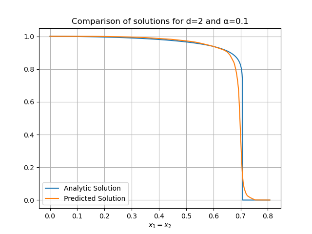
(a) $\alpha=0.1$

(b) $\alpha=1$

(c) $\alpha=1.9$

Figure 1. Two dimensional comparison of DNN and exact solution when $d=2$.

(a) $\alpha=0.1$

(b) $\alpha=1$

(c) $\alpha=1.9$

Figure 2. Three dimensional comparison of DNN and exact solution for $d=2$. In each Figure, left: exact solution, right: DNN solution.

In Figure 1 the most visible difference between the DNN and the solution (4.1) is near the boundary $\partial B(0,1)$, principally in the cases $\alpha=0.1$ and $\alpha=1.0$. This can also be seen in Figure 2, in the points where one component is near zero and the other component is near 1 or -1.

(a) $\alpha=0.1$

(b) $\alpha=1$

(c) $\alpha=1.9$

Figure 3. Two dimensional comparison of DNN and exact solution when $d=5$.

Now we set $d=5$. Figure 3 shows the comparative between the optimal DNN and the solution (4.1) for $\alpha=0.1,1,1.9$ in a grid of 5000 points between 0 and $\frac{1}{\sqrt{5}}+0.1$. The $x$-axis is the value of the components $x_{1}=...=x_{5}$. Figure 4 shows the comparative in 3D in a grid of 1000$\times$1000 points in $[-1,1]\times[-1,1]$. The $x$-axis is the value of $x_{1}=...=x_{4}$ and the $y$-axis is the value of $x_{5}$.

(a) $\alpha=0.1$

(b) $\alpha=1$

(c) $\alpha=1.9$

Figure 4. Three dimensional comparison of DNN and exact solution for $d=5$. In each Figure, left: exact solution, right: DNN solution.

As we can see in Figure 3 the approximation via DNN is good. The results have the most visible difference between the prediction and the solution is near the boundary $\partial B(0,1)$ for the three cases. In Figure 4 we see the same behavior that in the case $d=2$, that is, near 0 in the $x$-axis and near $\{-1,1\}$ in the $y$-axis there are a notable difference between the optimal DNN and the solution (4.1).

In order to improve the the approximation, we perform a study of the algorithm when we increase the number of iterations $M$ of the Monte Carlo simulation and the size of the training set $P$. In particular, for the same values of $\alpha$ as before, we calculate the elapsed time of the algorithm when $M=10,100,1000,2000$ and $P=10,100,1000,2000$. The results are shown in seconds in Tables 1(a), 1(b) and 1(c).

M\P	10	100	1000	2000
10	5.44	5.62	8.35	10.49
100	5.45	6.25	14.13	22.26
1000	5.94	12.46	70.90	139.47
2000	6.61	17.29	140.75	274.69

(a) $\alpha=0.1$

M\P	10	100	1000	2000
10	5.50	5.76	8.67	10.90
100	5.54	6.56	15.13	23.54
1000	6.47	13.32	79.53	151.38
2000	7.00	20.19	151.30	294.83

(b) $\alpha=1.0$

M\P	10	100	1000	2000
10	5.60	6.72	17.86	29.27
100	6.09	14.40	101.61	203.21
1000	18.27	101.77	981.54	2012.45
2000	22.54	197.30	2012.85	5556.19

(c) $\alpha=1.9$

Table 1. Example 1: Elapsed time in seconds of the SGD algorithm with $d=5$

As we can see in the three tables, the setting that takes the longest elapsed time is when $M=2000$ and $P=2000$. This seems reasonable because we need to do a more expensive Monte Carlo simulation for a larger number of points in $\mathbb{R}^{5}$.

Another relationship between elapsed time and PDE parameters can be seen in Tables 1(a), 1(b) and 1(c). In particular, for small values of $\alpha$ the algorithm takes less time than when $\alpha$ is larger.

Also, from Tables 1(a), 1(b) and 1(c), we can deduce that for fixed $M$, the value of the elapsed time when $P$ increases is similar to the value of the elapsed time when $M$ increases and $P$ is fixed.

Now, for the same values of $M$ and $P$, and for $\alpha=0.1,0.5,1,1.5,1.9$ the Figure 5 shows the mean square error calculated as in (3.6) for $5000$ random points in $D$. On the other hand, Figure 6 shows the mean relative error calculated as in (3.7) for the same $5000$ points in $D$.

(a) $P=10$

(b) $P=100$

(c) $P=1000$

(d) $P=2000$

Figure 5. Mean square error against number of Monte Carlo iterations $M$ for 5 values of $\alpha$.

(a) $P=10$

(b) $P=100$

(c) $P=1000$

(d) $P=2000$

Figure 6. Mean relative error against number of Monte Carlo iterations $M$ for 5 values of $\alpha$.

Notice from Figure 5 that for small values of $\alpha$, one needs big values of $P$. For example, when $\alpha=0.1$, $P=1000$ is not enough to have a mean square error of the order of $10^{-4}$, even with $M=2000$. On the other hand, when $\alpha=1.9$, $P=1000$ gives the order of $10^{-4}$ on the mean square error for $M\geq 100$ . Also notice that, despite that the high elapsed time when $P=2000$, in almost all the choices of $M$ and $\alpha$, this setting ensures a mean square error of the order of $10^{-3}$, and the order of $10^{-4}$ if $M$ is greater than $100$.

In Figure 6 we see that for the mean relative error is more difficult to obtain a value small order. In particular, only for $P\geq 1000$ we can ensure an error lower than the order $10^{-1}$ for almost all the choices of $M$ and $\alpha$. The excluding case is when $\alpha=1.9$, where the errors are greater than $10^{-1}$, but they are still in that order.

Finally, we set $d=15$ and we change the value of $\gamma$ to $5\times 10^{-4}$. In Figure 7 we compare the realization of the optimal DNN with the solution (4.1) for $\alpha=0.1,1,1.9$ in a grid of 5000 points between 0 and $\frac{1}{\sqrt{15}}+0.1$. The $x$-axis is the value of the components $x_{1}=...=x_{15}$. In Figure 8 we do the comparative in 3D in a grid of 1000$\times$1000 points in $[-1,1]\times[-1,1]$. The $x$-axis is the value of $x_{1}=...=x_{14}$ and the $y$-axis is the value of $x_{15}$.

(a) $\alpha=0.1$

(b) $\alpha=1$

(c) $\alpha=1.9$

Figure 7. Two dimensional comparison of DNN and exact solution when $d=15$.

(a) $\alpha=0.1$

(b) $\alpha=1$

(c) $\alpha=1.9$

Figure 8. Three dimensional comparison of DNN and exact solution for $d=15$. In each Figure, left: exact solution, right: DNN solution.

Notice from Figure 7 that the behavior is a quite similar that when $d=5$. In the sense that for all the values of $\alpha$, the optimal DNN is not a good prediction of the solution near the boundary $\partial B(0,1)$, specially when $\alpha=0.1$ and $\alpha=1.9$. Despite the not-so-good approximation mentioned above, in Figure 8 we see that the optimal DNN still preserves the solution’s form.

4.1.1. Comparison of loss functions

Recall from (4.1) the radiality of the solution in this example. As said before, in previous figures we perform the SGD algorithm with the loss function defined in (3.5). In this section we compare the optimal DNNs of the SGD algorithm for the two different losses described in Section 4. The comparison will be made for $\alpha=0.1,1,1.9$, $d=15$, $\gamma=5\times 10^{-4}$, $P=2000$, $L=400$ and $M=100$.

As we can see in Figure 9, the performance of the SGD algorithm is better when we are using the loss function (3.5) instead of function (3.4). Despite there are not so much difference between the errors obtained with both loss functions, in the visualization on Figure 9 is remarkable the use of the loss function with radial term.

(a) $\alpha=0.1$

(b) $\alpha=1$

(c) $\alpha=1.9$

Figure 9. Two dimensional comparison of two optimal DNN solutions with different loss functions, for $d=15$.

4.2. Example 2: Non constant source term

Let $d\geq 2$. Consider the following problem

$$\centering\begin{cases}(-\Delta)^{\frac{\alpha}{2}}u(x)&=b_{\alpha,d}\left(1-\left(1+\frac{\alpha}{d}\right)|x|^{2}\right)\qquad x\in B(0,1),\\ \hfill u(x)&=0\hfill x\notin B(0,1),\end{cases}\@add@centering$$ (4.2)

where

$$b_{\alpha,d}=2^{\alpha}\frac{\Gamma\left(\frac{\alpha}{2}+\frac{d}{2}\right)\Gamma\left(\frac{\alpha}{2}+2\right)}{\Gamma\left(\frac{d}{2}\right)}.$$

This problem has an explicit continuous solution $u$ given by [13].

$$u(x)=(1-\left\|x\right\|^{2})_{+}^{1+\frac{\alpha}{2}}.$$

For this example, is also radial, then the loss function (3.5) will be used. We consider $d=2$ and $d=5$. For both dimensions, we set $M=500$, $P=1000$, $L=200$, $\gamma=5\times 10^{-3}$ and $N_{Iter}=1000$.

First we set $d=2$. In Figure 10 we compare the realization of the optimal DNN with the solution (4.2) for $\alpha=0.5,1.5,1.9$ in a grid of 5000 points between 0 and $\frac{1}{\sqrt{2}}+0.1$. Figure 11 we do the comparative in 3D in a grid of 1000$\times$1000 points in $[-1,1]\times[-1,1]$.

(a) $\alpha=0.5$

(b) $\alpha=1.5$

(c) $\alpha=1.9$

Figure 10. Two dimensional comparison of DNN and exact solution when $d=2$.

(a) $\alpha=0.5$

(b) $\alpha=1.5$

(c) $\alpha=1.9$

Figure 11. Three dimensional comparison of DNN and exact solution for $d=2$. In each Figure, left: exact solution, right: DNN solution.

As in Example 1, the optimal DNN fits pretty well the solution (4.2) when $d=2$, for all studied cases of $\alpha$, but unlike in previous example, in this case there are no problems near the boundary and there are not major visible differences between the optimal DNN and the solution (4.2). On the other hand, Figure 11 shows that the optimal DNN has the same order and the same form of the analytical solution.

For $d=2$ we compare the elapsed time for different choices of $M$ and $P$. This was made for $\alpha=0.5$ (Table 2(a)), $\alpha=1.5$ (Table 2(b)) and for $\alpha=1.9$ (Table 2(c)). In those tables we can see that the elapsed time increases when we increase the value of $M$ and $P$. For fixed values of $M$ and $P$ the elapsed time also increases when we increases the value of $\alpha$, but the major gap is for larger values of $M$ and $P$.

M\P	10	100	1000	2000
10	3.75	3.77	5.40	6.66
100	3.71	4.35	10.39	16.61
1000	4.47	9.28	60.81	116.09
2000	4.71	14.99	120.82	227.46

(a) $\alpha=0.5$.

M\P	10	100	1000	2000
10	3.67	3.80	5.83	7.66
100	3.77	4.86	15.66	26.71
1000	5.02	14.30	113.68	219.76
2000	4.85	25.93	223.80	431.75

(b) $\alpha=1.5$.

M\P	10	100	1000	2000
10	3.67	4.08	8.53	12.94
100	4.04	6.95	42.65	80.22
1000	7.36	40.62	384.95	760.63
2000	13.30	77.12	755.87	1457.21

(c) $\alpha=1.9$.

Table 2. Example 2: Elapsed time in seconds of the SGD algorithm with $d=2$.

Finally we compare the mean square error and the mean relative error in a grid of the Monte Carlo iterations $M$, for each $\alpha\in\{0.1,0.5,1,1.5,1.9\}$ and $P=10,100,1000,2000$. The results are summarized in Figures 12 and 13.

(a) $P=10$

(b) $P=100$

(c) $P=1000$

(d) $P=2000$

Figure 12. Mean square error against number of Monte Carlo iterations $M$ for 5 values of $\alpha$.

(a) $P=10$

(b) $P=100$

(c) $P=1000$

(d) $P=2000$

Figure 13. Mean relative error against number of Monte Carlo iterations $M$ for 5 values of $\alpha$.

Figure 12 shows that the mean square error decreases when we increases $P$ and $M$, achieving the order $10^{-4}$ for the cases $P=1000$ and $P=2000$ when $M\geq 100$ and for any value of $\alpha$. In Figure 13 we see a pretty similar behavior of the mean relative error than the MSE, but with different order: for $P=1000$ and $P=2000$, we have an error of order $10^{-1}$ only for small values of $\alpha$, $\alpha\leq 1$, and for $\alpha>1$, only in the case $M=1000$. For the other cases, the MRE is greater than 1. In other words, the mean square error is small for all the studied values for $\alpha$, but only for small values of $\alpha$ we reach a small value on the mean relative error.

Now we set $d=5$. We will compare the optimal DNN and the solution (4.2) in 2D (Figure 14) and in 3D (Figure 15) for $\alpha=0.5,1.5,1.9$. This will be done in the same way as in Example 1. In both Figures we can see a good approximation of the solution (4.2) with the optimal DNN obtained with the SGD algorithm. In the three settings of $\alpha$ the most visible difference of the approximation is near the center of the domain, i.e, near 0, and near the boundary $\partial B(0,1)$, specially in the cases $\alpha=1.5$ and $\alpha=1.9$. Moreover, Figure 15 shows that the form of the optimal DNN is the same of the solution (4.2).

(a) $\alpha=0.5$

(b) $\alpha=1.5$

(c) $\alpha=1.9$

Figure 14. Two dimensional comparison of DNN and exact solution when $d=5$.

(a) $\alpha=0.5$

(b) $\alpha=1.5$

(c) $\alpha=1.9$

Figure 15. Three dimensional comparison of DNN and exact solution for $d=5$. In each Figure, left: exact solution, right: DNN solution.

4.3. Example 3: Non zero boundary term

Let $d\geq 2$ and recall that $D=B(0,1)$. For $y\in D^{c}$ fixed let the boundary condition $g$ be a translation of the fundamental solution of the fractional Laplacian, that is,

$$g(x)=\frac{\Gamma\left(\frac{d}{2}-\frac{\alpha}{2}\right)}{2^{\alpha}\pi^{\frac{d}{2}}\Gamma\left(\frac{\alpha}{2}\right)}|x-y|^{\alpha-d}.$$

Now consider the problem

$$\centering\begin{cases}(-\Delta)^{\frac{\alpha}{2}}u(x)&=0\hfill x\in B(0,1),\\ \hfill u(x)&=g(x)\qquad x\notin B(0,1).\end{cases}\@add@centering$$ (4.3)

From the choice of $y$ outside $B(0,1)$, one obtains that one exact solution for previous problem is $u(x)=g(x)$ for every $x\in\mathbb{R}^{d}$. In this particular case, we consider the vector $y=(2,0,...,0)\in\mathbb{R}^{d}$.

For this example, we will set the values $M=300$, $P=1000$, $L=200$, $\gamma=5\times 10^{-3}$ and $N_{Iter}=1000$. First we study the algorithm in dimension 2. Figure 16 shows the comparison of the optimal DNN and the solution of problem (4.3) for $\alpha=0.5,1.5,1.9$ in a grid made in the same way as in previous examples. Figure 17 shows the comparison in 3D.

From Figure 16 we can see a poorly approximation of the optimal DNN when $\alpha=0.5$. The approximation is improved by increasing $\alpha$. By de order of the solution of (4.3), we see that the optimal DNN still preserves the form of the analytic solution in the square $[-1,1]\times[-1,1]$.

(a) $\alpha=0.5$

(b) $\alpha=1.5$

(c) $\alpha=1.9$

Figure 16. Two dimensional comparison of DNN and exact solution when $d=2$.

(a) $\alpha=0.5$

(b) $\alpha=1.5$

(c) $\alpha=1.9$

Figure 17. Three dimensional comparison of DNN and exact solution for $d=2$. In each Figure, left: exact solution, right: DNN solution.

Now we study the elapsed time by changing the values of $M$ and $P$ for $\alpha=0.5,1.5,1.9$. The elapsed times are shown in Tables 3(a), 3(b) and 3(c).

M\P	10	100	1000	2000
10	3.64	3.78	5.36	6.54
100	3.71	4.30	9.99	15.98
1000	4.31	9.21	58.56	113.46
2000	4.98	15.64	111.57	219.05

(a) $\alpha=0.5$.

M\P	10	100	1000	2000
10	3.71	3.83	5.84	7.62
100	3.76	4.84	15.27	26.80
1000	4.61	15.62	115.40	216.40
2000	5.50	26.18	216.27	423.64

(b) $\alpha=1.5$.

M\P	10	100	1000	2000
10	3,69	4.06	8.52	12.94
100	4.02	7.49	41.39	81.52
1000	6.87	41.88	387.11	768.78
2000	9.99	70.84	750.55	1486.86

(c) $\alpha=1.9$.

Table 3. Example 3: Elapsed time in seconds of the SGD algorithm with $d=2$.

From those values of $M$ and $P$, and for $\alpha=0.1,0.5,1,1.5,1.9$ we calculate the mean square error and the mean relative error of the optimal DNN. These errors are in Figure 18 and 19.

Figure 18 shows a small mean square error in all settings of $M$, $P$ and $\alpha$, but this small error is a bit tricky, because for small values of $\alpha$, the order of the solution is also small.

The errors shown in Figure 19 are very different of errors in Figure 18. Figure 19 shows an error near of (or lower than) the order $10^{0}$ for the cases $\alpha=0.1,0.5$. When $\alpha=1$, for larger values of $M$ and $P$ we have an error lower than the order $10^{-2}$, but in the other cases, the error is also near of the order $10^{-1}$. The lowest errors are in the cases of $\alpha=1.5$ and $\alpha=1.9$. The error is of the order $10^{-3}$ for large values of $M$ and $P$, and near of the order $10^{-2}$ for small values of $M$ and $P$.

(a) $P=10$

(b) $P=100$

(c) $P=1000$

(d) $P=2000$

Figure 18. Mean square error against number of Monte Carlo iterations $M$ for 5 values of $\alpha$.

(a) $P=10$

(b) $P=100$

(c) $P=1000$

(d) $P=2000$

Figure 19. Mean relative error against number of Monte Carlo iterations $M$ for 5 values of $\alpha$.

4.4. Example 4: A counter example for the algorithm

Let $d\geq 2$ and $D=B(0,1).$ Consider the following problem

$$\centering\begin{cases}(-\Delta)^{\frac{\alpha}{2}}u(x)&=0\hfill x\in B(0,1),\\ \hfill u(x)&=\displaystyle\sum_{i=1}^{d}x_{i}\qquad x\notin B(0,1),\end{cases}\@add@centering$$ (4.4)

Property 2 in [24] ensures that every harmonic function must be $\alpha$-harmonic for all $\alpha\in(0,2)$. In particular, the function

$$g(x)=\sum_{i=1}^{d}x_{i},\qquad x\notin B(0,1),$$

is harmonic, and then it is $\alpha$-harmonic. Therefore, for all $\alpha\in(0,2)$, the solution of problem (4.4) is

$$u(x)=\sum_{i=1}^{d}x_{i},\qquad x\in\mathbb{R}^{d}.$$

For this Example we only consider dimension 2. The performances of the algorithm are similar for different choices of $d$. Figure 20 shows a comparison between the optimal DNN and the solution of problem (4.4) in two dimensions. Figure 21 shows the same comparison, but in three dimensions.

(a) $\alpha=0.5$

(b) $\alpha=1.5$

(c) $\alpha=1.9$

Figure 20. Two dimensional comparison of DNN and exact solution when $d=2$.

(a) $\alpha=0.5$

(b) $\alpha=1.5$

(c) $\alpha=1.9$

Figure 21. Three dimensional comparison of DNN and exact solution for $d=2$. In each Figure, left: exact solution, right: DNN solution.

We can notice from Figures 20 and 21 that for almost all the settings of $\alpha$, the algorithm does not perform a good approximation of the solution of problem (4.4). We only have a well approximation when $\alpha$ is near 2.

5. Conclusion and discussion

In this section we talk about conclusions and discussions about our proposed algorithm and its behavior.

First of all we will highlight the behavior of the WoS process. For small values of $\alpha$, the isotropic $\alpha$-stable process exits far from the boundary $\partial B(0,1)$. This implies that the WoS process exits the set $D$ in a few steps, that means, the value of $N$ is also small.

On the other hand, when $\alpha$ is near 2 (i.e. $\alpha$ is large), the isotropic $\alpha$-stable process exits very close to the boundary $\partial B(0,1)$. This means that the WoS process needs more steps to exit the set $D$. In other words, the value of $N$ is large. This makes sense, because in the case $\alpha=2$, one can see in [16, 25] that the WoS process in this case never exits the set $D$, and then the value of $N$ is infinite a.s.

In terms of time, we note that the previously mentioned behavior of the WoS process has a strong influence in the elapsed time of the SGD algorithm. Indeed, we can see in the different tables on each example that for the same values of $P$ and $M$, the algorithm takes more time for large values of $\alpha$ than for small ones.

Notice also that in all the examples, there is a good approximation for large values of $\alpha$. In the case of small values of $\alpha$, the approximation has some issues, specially in the examples where the boundary condition is non-zero. This problem is caused principally due the same behavior of the WoS pocess: If $\alpha$ is small, the last element in the WoS process, namely $\rho_{N}$, is a point far away the set $D$, and if the boundary condition is non-zero, the Monte Carlo iterations have the terms involving $g(\rho_{N})$. This leads to many errors if a small number of Monte Carlo iterations are considered, that is our case. This has not happened in [25], because the order of the Monte Carlo iterations in that paper is much higher ($2^{10}$ iterations) compared to the order considered in this paper (maximum 2000 iterations).

We want to emphasize the principal advantage of this numerical method. With this method we can estimate the value of the solution of the fractional PDE in every point of $\mathbb{R}^{d}$ once the deep neural network is trained, contrary to the case of Monte Carlo, where we need to do a different Monte Carlo realization for each point of $\mathbb{R}^{d}$, and that is an expensive computation. The same happens in the case of finite differences, where we know the value of the solution only on a grid, and the computational cost is larger the finer grid is. For this method, and in the examples presented, we only needed a small number of Monte Carlo iterations, for a given set of points on $\mathbb{R}^{d}$, with maximum size of $2000$.

References

- [1] G. Acosta and J. P. Borthagaray. A fractional Laplace equation: regularity of solutions and finite element approximations. SIAM Journal on Numerical Analysis, 55(2), 472-495, 2017.
- [2] C. Beck, F. Hornung, M. Hutzenthaler, A. Jentzen, and T. Kruse. Overcoming the curse of dimensionality in the numerical approximation of Allen–Cahn partial differential equations via truncated full-history recursive multilevel picard approximations. Journal of Numerical Mathematics, 28(4):197–222, dec 2020.
- [3] J. Berner, P. Grohs and A. Jentzen. Analysis of the generalization error: Empirical risk minimization over deep artificial neural networks overcomes the curse of dimensionality in the numerical approximation of Black–Scholes partial differential equations. SIAM Journal on Mathematics of Data Science, 2(3), 631-657, 2020.
- [4] R. Blumenthal, R. Getoor and D. Ray. On the Distribution of First Hits for the Symmetric Stable Processes. Transactions of the American Mathematical Society, 99(3), 540–554, 1961. https://doi.org/10.2307/1993561.
- [5] A. Bonito, J. P. Borthagaray, R. H. Nochetto, E. Otárola and A. J. Salgado. Numerical methods for fractional diffusion. Computing and Visualization in Science, 19(5), 19-46, 2018.
- [6] L. Caffarelli, and L. Silvestre, An extension problem related to the fractional Laplacian, Comm. Partial Differential Equations 32 (2007), no. 7-9, 1245–1260.
- [7] J. Castro. Deep Learning schemes for parabolic nonlocal integro-differential equations. Partial Differ. Equ. Appl. 3, no. 6, 77, 2022.
- [8] J.Castro, C. Muñoz and N. Valenzuela. The Calderón’s problem via DeepONets. arXiv preprint arXiv:2212.08941, 2022.
- [9] T. Chen and H. Chen. Universal approximation to nonlinear operators by neural networks with arbitrary activation functions and its application to dynamical systems. IEEE Transactions on Neural Networks, 6(4):911–917, 1995.
- [10] T. De Ryck and S. Mishra. Error Analysis for Physics-Informed Neural Networks (PINNs) Approximating Kolmogorov PDEs. Advances in Computational Mathematics, vol. 48, no. 6, Nov. 2022. https://doi.org/10.1007/s10444-022-09985-9.
- [11] T. De Ryck, A. D. Jagtap and S. Mishra. Error estimates for physics informed neural networks approximating the Navier-Stokes equations. arXic preprint arXiv:2203.09346, 2022.
- [12] B. Dyda, A. Kuznetsov and M. Kwaśnicki Fractional Laplace Operator and Meijer G-Function. Constructive Approximation, vol. 45, no. 3, Apr. 2016, pp. 427–48.
- [13] B. Dyda. Fractional calculus for power functions and eigenvalues of the fractional Laplacian. Fractional Calculus and Applied Analysis, vol. 15, no. 4, 2012, pp. 536-555. https://doi.org/10.2478/s13540-012-0038-8
- [14] W. E, J. Han and A. Jentzen. Deep learning-based numerical methods for high-dimensional parabolic partial differential equations and backward stochastic differential equations. Commun. Math. Stat. 5(4), 349–380, 2017.
- [15] D. Elbrächter, D. Perekrestenko, P. Grohs, and H. Bölcskei. Deep Neural Network Approximation Theory. IEEE Transactions on Information Theory, vol. 67, no. 5, May 2021, pp. 2581–623. https://doi.org/10.1109/tit.2021.3062161.
- [16] P. Grohs and L. Herrmann. Deep neural network approximation for high-dimensional elliptic PDEs with boundary conditions. IMA Journal of Numerical Analysis, 2021. https://doi.org/10.1093/imanum/drab031.
- [17] M. Gulian, and G. Pang. Stochastic solution of elliptic and parabolic boundary value problems for the spectral fractional Laplacian. arXiv preprint arXiv:1812.01206, 2018.
- [18] M. Gulian,, M. Raissi, P. Perdikaris and G. Karniadakis. Machine Learning of Space-Fractional Differential Equations. SIAM Journal on Scientific Computing, vol. 41, no. 4, Jan. 2019, pp. A2485–509. https://doi.org/10.1137/18m1204991.
- [19] J. Han, A. Jentzen and W. E. Solving High-Dimensional Partial Differential Equations Using Deep Learning. Proceedings of the National Academy of Sciences, vol. 115, no. 34, Aug. 2018. https://doi.org/10.1073/pnas.1718942115.
- [20] J. Havil. Gamma: Exploring Euler’s Constant. Princeton University Press, 2003.
- [21] C. Huré, H. Pham, and X. Warin. Deep backward schemes for high-dimensional nonlinear PDEs, Math. Comp. 89, no. 324, 1547–1579, 2020.
- [22] M. Hutzenthaler, A. Jentzen, Thomas Kruse, Tuan Anh Nguyen, A proof that rectified deep neural networks overcome the curse of dimensionality in the numerical approximation of semilinear heat equations, Partial Differ. Equ. Appl. 1, 10 (2020).
- [23] M Hutzenthaler, A. Jentzen, T. Kruse, T. A. Nguyen, and P. Von Wurstemberger. Overcoming the curse of dimensionality in the numerical approximation of semilinear parabolic partial differential equations. Proceedings of the Royal Society A: Mathematical, Physical and Engineering Sciences, 476(2244):20190630, dec 2020.
- [24] M. Itô. On -Harmonic Functions. Nagoya Mathematical Journal, 26, 205-221. 1966.
- [25] A. E Kyprianou, A. Osojnik and T. Shardlow, Unbiased ‘walk-on-spheres’ Monte Carlo methods for the fractional Laplacian, IMA Journal of Numerical Analysis, Volume 38, Issue 3, July 2018, pp 1550–1578, https://doi.org/10.1093/imanum/drx042.
- [26] A. Lischke, G. Pang, M. Gulian, F. Song, C. Glusa, X. Zheng, … and G. E. Karniadakis. What is the fractional Laplacian?. arXiv preprint arXiv:1801.09767, 2018.
- [27] L. Lu, P. Jin and G. Em Karniadakis. Learning Nonlinear Operators via DeepONet Based on the Universal Approximation Theorem of Operators. Nature Machine Intelligence, vol. 3, no. 3, Mar. 2021. https://doi.org/10.1038/s42256-021-00302-5.
- [28] K. O. Lye, S. Mishra, and D. Ray. Deep learning observables in computational fluid dynamics. Journal of Computational Physics, page 109339, 2020.
- [29] K. O. Lye, S. Mishra, D. Ray, and P. Chandrashekar. Iterative surrogate model optimization (ISMO): An active learning algorithm for pde constrained optimization with deep neural networks. Computer Methods in Applied Mechanics and Engineering, 374:113575, 2021
- [30] M. Raissi, P. Perdikaris, and G. E. Karniadakis, Machine learning of linear differential equations using Gaussian processes, J. Comput. Phys., 348 (2017), pp. 683–693, https://doi.org/10.1016/j.jcp.2017.07.050.
- [31] N. Valenzuela. A new approach for the fractional Laplacian via deep neural networks. arXiv preprint arXiv:2205.05229, 2022.