Random free-fermion quantum spin chain with multispin interactions

Abstract

We study the effects of quenched disorder in a class of quantum chains with ($p+1$)-multispin interactions exhibiting a free fermionic spectrum, paying special attention to the case $p=2$. Depending if disorder couples to (i) all the couplings or just to (ii) some of them, we have two distinct physical scenarios. In case (i), we find that the transitions of the model are governed by a universal infinite-randomness critical point surrounded by quantum Griffiths phases similarly as happens to the random transverse-field Ising chain. In case (ii), we find that quenched disorder becomes an irrelevant perturbation: the clean critical behavior is stable and Griffiths phases are absent. Beyond the perturbative regime, disorder stabilizes a line of finite-randomness critical points (with nonuniversal critical exponents), that ends in a multicritical point of infinite-randomness type. In that case, quantum Griffiths phases also appear surrounding the finite-disorder transition point. We have characterized the correlation functions and the low-temperature thermodynamics of these chains. Our results are derived from a strong-disorder renormalization-group technique and from finite-size scaling analysis of the spectral gap computed exactly (up to sizes $\sim 10^{7}$) via an efficient new numerical method recently introduced in the literature [Phys. Rev. B 104, 174206 (2021)].

Published in Phys. Rev. B 108, 214413 (2023); DOI: 10.1103/PhysRevB.108.214413

I Introduction

The importance of studying one-dimensional quantum models is invaluable. Due to the peculiarities of the phase space in $d=1$, many models can be precisely described and, thus, serve as important test beds for physical insights (Giamarchi, 2004). Among those models, there is an important class that goes under the general name of free systems. These are systems (of volume $V$) whose the exponentially large Hilbert space of dimension $\sim e^{V}$ can be expressed as a combination of $\sim V$ quasienergies of a free-particle system. Despite the name, they exhibit nontrivial phenomena, such as phase transitions and zero-energy fractional edge modes, and are, thus, good starting points to understand many complex behaviors of more general systems (Lieb et al., 1961; Pfeuty, 1970; Kitaev, 2001).

Initially, the known free systems models were linked to a Jordan-Wigner transformation which maps interacting spin models into free fermionic particles, i.e., into models which are bilinear in the fermionic operators or fields. Later, it was realized that the existence of this transformation is not a necessary condition (Baxter, 1989). It is possible to construct the eigen-spectrum of the spin system from the free-fermion pseudo-energies obtained from the roots of a characteristic polynomial. This polynomial is constructed thanks to the infinite number of conserved charges of the model (Fendley, 2019; Alcaraz and Pimenta, 2020a, b). Interestingly, these latter free systems, a priori, cannot be written in term of local bilinears of fermion operators.

The first models in this class are the $\text{Z}_{N}$-symmetric free parafermionic models (Baxter, 1989, 1989, 2004; Fendley, 2014) and the three-spin interacting Fendley model (Fendley, 2019). Actually, it has been found that Fendley model belongs to a large family of spin chains with multispin interactions and $\text{Z}_{N}$-symmetry (Alcaraz and Pimenta, 2020a, b). For $N>2$, the spectrum is complex and has a free parafermionic form. Furthermore, it was shown that the free-particle pseudo-energies of some of the above models are also the pseudo-energies of a multispin U(1) symmetric XY model (Alcaraz et al., 2021; Alcaraz and Pimenta, 2021). Additional developments related to Fendley model can be found in Refs. (Elman et al., 2021; Miao, 2022; Alcaraz et al., 2023; Chapman et al., 2023).

Recently, it was shown that, in general, the roots of the characteristic polynomial yielding the free fermionic spectrum can be efficiently obtained numerically (Alcaraz et al., 2021). As a consequence, the finite-size gaps of the spin system can be computed straightforwardly for quite large system sizes. Furthermore, the numerical cost for exactly computing the finite-size gap with machine precision (and, hence, the associated dynamical critical exponent) is minimum at criticality increasing only linearly with the chain size. While this may seems innocuous for translation-invariant systems where analytical results can often be obtained, it is of great applicability to quenched disordered systems where analytical results are scarce and exactly numerical results are plagued by numerical instabilities inherent to the extreme slow critical dynamics of these systems (Getelina and Hoyos, 2020). This brings us to the topic of our research. What are the effects of quenched disorder on these generalized free fermionic systems?

It is well known that the effects of quenched disorder (i.e., static random inhomogeneities) in strongly interacting systems can lead to interesting new phenomena. For instance, even the small amount of inhomogeneities can change the singular behavior of a critical system (Harris, 1974; Vojta and Hoyos, 2014), change the sharp character of a transition by smearing (Vojta, 2003; Hoyos and Vojta, 2008, 2012), or even destroy the phase transition itself (Imry and Ma, 1975; Imry and Wortis, 1979). For reviews, see, e.g., Refs. Vojta, 2006, 2010.

In the (free fermionic) transverse-field Ising chain, quenched disorder completely changes the critical behavior of the clean (homogeneous) system as expected from the Harris criterion (Harris, 1974). The conventional critical dynamical scaling of the clean system $\tau\sim\xi^{z}$ (with $\tau$ and $\xi$ being, respectively, time and length scales, and $z=1$ being the dynamical exponent) is replaced by an activated dynamical scaling $\ln\tau\sim\xi^{\psi}$ (with universal, i.e., disorder-independent, tunneling exponent $\psi=1/2$), which is now recognized as a hallmark of the so-called infinite-randomness quantum criticality (Fisher, 1992, 1995). Technically, this means that the disorder-induced statistical fluctuations among the relevant energy scales increases without bounds under the renormalization-group coarse-grain procedure. Additionally, it was realized that this exotic phenomena appears in all dimensions (Senthil and Sachdev, 1996; Pich et al., 1998; Kovács and Iglói, 2011) and in many other contexts, such as in Heisenberg-like quantum chains and ladders (Fisher, 1994; Boechat et al., 1996; Monthus et al., 1997; Refael et al., 2002; Damle and Huse, 2002; Yusuf and Yang, 2003; Hoyos and Miranda, 2004a, b; Bonesteel and Yang, 2007; Hrahsheh et al., 2012; Quito et al., 2015, 2016; Shu et al., 2016; Quito et al., 2019, 2020), in the Hubbard chain (Mélin and Iglói, 2006; Yu et al., 2022), in aperiodic quantum chains (Vieira, 2005a, b; Filho et al., 2012; Casa Grande et al., 2014), in open quantum rotors systems (Hoyos et al., 2007a; Vojta et al., 2009), in reaction-diffusion models such as the contact process (Hooyberghs et al., 2003, 2004; Vojta and Dickison, 2005; Hoyos, 2008; Vojta, 2012; Vojta and Hoyos, 2015; Fiore et al., 2018), in unbiased random walkers in random media (Fisher et al., 1998), and in Floquet criticality (Monthus, 2017; Berdanier et al., 2018). For a review, see, e.g., Refs. Iglói and Monthus, 2005, 2018. Despite these overwhelming situations in which infinite-randomness is theoretically found, experimental evidence is slight (Guo et al., 2008; Ubaid-Kassis et al., 2010; Demkó et al., 2012; Xing et al., 2015; Lewellyn et al., 2019).

Despite all the progress on characterizing the infinite-randomness criticality, we currently do not know what are the necessary conditions ensuring its appearance. It is then desirable to further study other aspects which were not considered in the previous studies. Here, we consider interactions involving more than the conventional two-body interactions. We pay special attention to the $\text{Z}_{2}$-symmetric free fermionic case in which the interactions involve three consecutive spins (Fendley, 2019). The clean phase diagram has three critical lines separating three gapful phases which are related to each other by triality. The universality classes of the associated transitions are that of the transverse-field Ising chain, but that of the multicritical point (where these three critical lines meet) is yet to be determined. Currently, only its dynamical critical exponent $z=\frac{3}{2}$ (Fendley, 2019) and the specific-heat exponent $\alpha=0$ (Alcaraz and Pimenta, 2020b) are known. An inhomogeneous quantum Ising chain sharing the same energy spectrum of this multicritical point was introduced in Ref. Alcaraz et al., 2023. In this related Ising chaing the order-parameter exponent is $\beta=\frac{1}{8}$ like the standard Ising chain.

Similarly to the random transverse-field Ising chain and to the spin-1/2 XX chain with random couplings, we show in this paper that generic quenched disorder stabilizes quantum Griffiths phases surrounding the three transition lines. In addition, the corresponding universality classes of these transitions and that of the multicritical point are the same and are of infinite-randomness type (with disorder-independent tunneling exponent $\psi=\frac{1}{2}$). Our results are based on a generalization of the strong-disorder renormalization-group (SDRG) method (Ma et al., 1979; Dasgupta and Ma, 1980; Bhatt and Lee, 1982) and on exact numerical calculations of the spectral gap using the aforementioned method based on the characteristic polynomial that allows us to obtain exact numerical results for very large lattice sizes (Alcaraz et al., 2021). After unveiling the structure of the SDRG flow, we generalize our results to the case of ($p+1$)-multispin interactions ($p=1,2,3,\dots$) and arrive basically at the same conclusions. All the transitions are in the same universality class of infinite-randomness type with the same tunneling exponent $\psi=\frac{1}{2}$.

In addition, we have also studied the case in which disorder couples only to one type of coupling constants (the others remaining homogeneous). In that case, some of the clean transition lines remain stable for weak disorder strength while a line of finite-disorder fixed points (with nonuniversal dynamical critical exponents $z)$ appear for large disorder strengths, and terminates in an infinite-randomness multicritical point.

This paper is organized as follows. In Sec. II we define the model studied and review some key results important to our purposes. In Sec. III we overview the expected effects of quenched disorder in a heuristic way. Our arguments are mostly based on the effects caused by rare-regions in the near-critical Griffiths phases. In Sec. IV we review the SDRG method for the standard 2-spin interacting case and generalize it to the 3-spin interacting case. In Sec. V we report our numerical study of the finite-size gap statistics of the model which are in agreement with the SDRG results. We present further discussions and concluding remarks in Sec. VI. Finally, the details of the renormalization-group flow are presented in Appendices A and B.

II The model and review of key results

We consider the $\left(p+1\right)$-multispin interacting quantum chains $\left(p=1,2,3,\dots\right)$, whose Hamiltonian, introduced in Refs. Alcaraz and Pimenta, 2020a, b, is given by

$${\cal H}_{p} = -\sum_{i=1}^{L-p}\lambda_{i}\sigma_{i}^{x}\prod_{j=i+1}^{i+p}\sigma_{j}^{z}-\sum_{i=L-p+1}^{L}\lambda_{i}\sigma_{i}^{x}\prod_{j=i+1}^{L}\sigma_{j}^{z}$$ (1)

$$= -\sum_{i=1}^{L}\lambda_{i}h_{i},\mbox{ where }h_{i}=-\sigma_{i}^{x}\prod_{j=i+1}^{\min\{i+p,L\}}\sigma_{j}^{z},$$ (2)

$\sigma_{i}^{x,y}$ are Pauli matrices associated with spin-$\frac{1}{2}$ degrees of freedom at site $i$, and $L$ is the total number of $\left\{h_{i}\right\}$ energy-density operators (which is also the total number of spins in the chain). The case $p=1$ is equivalent (up to global degeneracies) to the inhomogeneous transverse-field Ising quantum chain. The local interaction operator $h_{i}$ involves $\min\left\{p+1,i\right\}$ spins and satisfy the algebra (for $i\neq j$)

$$\left\{h_{i},h_{j}\right\}=0,\mbox{ if }\left|i-j\right|\leq p,\mbox{ and }\left[h_{i},h_{j}\right]=0\mbox{ otherwise}.$$ (3)

In other words, $h_{i}$ and $h_{j}$ commute if they are farther than $p$ lattice units ($\left|i-j\right|>p$), and anticommute otherwise. Evidently, from Eq. (1), $h_{i}^{2}=\mathds{1}$. Finally, $\lambda_{i}$ is the local multispin energy coupling. In this work, we introduce quenched disorder by considering $\left\{\lambda_{i}\right\}$ as independent random variables. Their precise distribution will be defined later.

Interestingly, it was shown (Alcaraz and Pimenta, 2020a, b) that the spectrum of (1) has the free fermionic form

$$E^{\left\{s_{k}\right\}}=-\sum_{k=1}^{\bar{L}}s_{k}\epsilon_{k},$$ (4)

where $s_{k}=\pm 1$, and the free fermionic pseudo-energies $\epsilon_{k}=1/\sqrt{x_{k}}$, with $\left\{x_{k}\right\}$ being the roots of the polynomial of degree $\bar{L}=\left\lfloor\frac{L+p}{p+1}\right\rfloor$ (with $\left\lfloor x\right\rfloor$ being the integer part of $x$):

$$P_{L}(x)=\sum_{\ell=0}^{\bar{L}}C_{L}\left(\ell\right)x^{\ell},$$ (5)

whose coefficients $C_{L}\left(\ell\right)$ are obtained from the recurrence relation

$$P_{L}(x)=P_{L-1}(x)-x\lambda_{L}^{2}P_{L-p-1}(x),$$ (6)

with the initial condition $P_{j}(x)=1$ for $j\leq 0$.

It is important to notice that the free fermionic character is guaranteed when open boundary conditions are applied. For other boundary conditions, very likely this is not true (Alcaraz and Pimenta, 2020a, b), and the solution of the model remains an open problem.

The first gap in the spectrum energy is $\Delta=2/\sqrt{x_{\text{max}}}$, where $x_{\text{max}}=\max\left\{x_{k}\right\}$ is the largest root of the polynomial (5). At and near criticality, it was recently shown (Alcaraz et al., 2021) that $x_{\text{max}}$ can be efficiently computed for very large chains even though $C_{L}\left(\ell\right)$ grows factorially with $\ell$. (Indeed, there is no need to compute all $C_{L}\left(\ell\right)$.) This is accomplished when one uses the Laguerre’s upper bound (LB) for the roots of a polynomial

$$x_{\text{LB}}=-\frac{\alpha_{1}}{\bar{L}}+\frac{\bar{L}-1}{\bar{L}}\sqrt{\alpha_{1}^{2}-2\left(\frac{\bar{L}}{\bar{L}-1}\right)\alpha_{2}},$$ (7)

where

$$\alpha_{1}=\frac{C_{L}(\bar{L}-1)}{C_{L}(\bar{L})},\mbox{ and }\alpha_{2}=\frac{C_{L}(\bar{L}-2)}{C_{L}(\bar{L})},$$ (8)

as the starting initial guess for the $x_{\text{max}}$.

In the (critical) homogeneous case $\lambda_{i}=\lambda$, it was shown (Alcaraz et al., 2021) that, for any $p$, the quantity $\Delta_{\text{LB}}\equiv 2/\sqrt{x_{\text{LB}}}=\left(1-\epsilon\right)\Delta$ as $L\rightarrow\infty$, with $0<\epsilon<1$ being a constant. Thus, $\Delta_{\text{LB}}$ has the same finite-size scaling properties of the finite-size gap $\Delta$ and, thus, can be used to obtain the dynamical critical exponent $z$, i.e.,

$$\Delta_{\text{LB}}\sim L^{-z_{\text{LB}}},$$ (9)

with $z_{\text{LB}}=z=\frac{p+1}{2}$ (Alcaraz and Pimenta, 2020a, b). Numerically, this is convenient since $\Delta_{\text{LB}}$ can be efficiently computed.

For $p=1$, it was shown (Alcaraz et al., 2021) that, in the critical quenched disordered case ($\left\{\lambda_{i}\right\}$ being independent and identically distributed random variables), $\Delta_{\text{LB}}=\left(1-\epsilon_{L}\right)\Delta$ with $\epsilon_{L}$ vanishing slowly as $L\rightarrow\infty$. This provides a convenient tool to obtain the dynamical scaling relation. In this case,

$$\ln\Delta_{\text{LB}}\sim-L^{\psi},$$ (10)

with universal tunneling exponent $\psi=1/2$. By universal we mean that $\psi$ does not depend on the particular distribution of the disorder variables. This result is expected since the model Hamiltonian (1) for $p=1$, apart from global degeneracies, has the same spectrum as the transverse-field Ising chain. It is worthy noting that the activated dynamical scaling (10) has been confirmed by many analytical and numerical studies (Iglói and Monthus, 2005). In addition, $\Delta_{\text{LB}}$ can also be used to study the finite-size gap in the near critical Griffiths phase. In this phase, the system is gapless even though it is short-range correlated (finite spin-spin correlation length) (Fisher, 1995). The finite-size gap $\Delta$ and the associated LB estimate, $\Delta_{\text{LB}}$, obeys the power-law scaling (9) with $z$ being the off-critical (Griffiths) dynamical exponent which depends on the distance from criticality. As criticality is approached, the off-critical dynamical exponent increases and becomes infinite at the critical point, in accordance to the activated critical dynamical scaling (10).

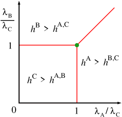
Figure 1: The phase diagram of the clean Hamiltonian (1) for $p=2$. Here, $\lambda_{3i-2}=\lambda_{A}$, $\lambda_{3i-1}=\lambda_{B}$, and $\lambda_{3i}=\lambda_{C}$. The solid red dashed lines are transitions in the Ising universality class ($z=1$). The multicritical point $\lambda_{A}=\lambda_{B}=\lambda_{C}$ is in a different universality class where $z=\frac{3}{2}$ and $\alpha=0$. The three phases are gapful and are similar to each other (see text).

The model (1) for $p=2$ and nondisordered couplings was studied in Ref. Fendley, 2019 for couplings of period $3$ [which is the natural period given by the algebra (3)], i.e.,

$$\lambda_{3i-2}=\lambda_{A},\ \lambda_{3i-1}=\lambda_{B},\mbox{ and }\lambda_{3i}=\lambda_{C}.$$ (11)

Exploring the triality of the model, the phase diagram was determined (see Fig. 1).

We now want to discuss what we mean by triality in this model. In the bulk limit, the lattice translations $i\rightarrow i+1$ (equivalent to $A\rightarrow B\rightarrow C\rightarrow A$) and $i\rightarrow i+2$ (equivalent to $A\rightarrow C\rightarrow B\rightarrow A$), and the lattice reflection $\left(i\rightarrow L+1-i\right)$ do not change the algebra (3) and, therefore, the spectrum. Thus,

$${\cal H}\left(\lambda_{A},\lambda_{B},\lambda_{C}\right) = {\cal H}\left(\lambda_{B},\lambda_{C},\lambda_{A}\right)={\cal H}\left(\lambda_{C},\lambda_{A},\lambda_{B}\right)$$ (12)

$$= {\cal H}\left(\lambda_{C},\lambda_{B},\lambda_{A}\right).$$

Now, consider the case $\alpha=\lambda_{A}/\lambda_{C}<1$ fixed. If the transition happens at $\beta=\lambda_{B}/\lambda_{C}\neq 1$, the relation (12) implies the existence of another transition at $\beta^{-1}$ for the same $\alpha$. Since there is only a global $\text{Z}_{2}$ symmetry to be broken, then there is only a single phase transition. Therefore, the transition must happen at $\beta_{c}=\beta_{c}^{-1}=1$. Successive applications of the relation (12) imply that the self-triality curves (red lines in Fig. 1) are the transition lines. Notice that this argument can be generalized to higher values of $p$ where the self-$\left(p+1\right)$-ality hyperplanes are the transition manyfolds. For $p=3$, see Ref. Elman et al., 2021.

The three different phases are characterized by the following expectation values: $h^{A}=\left|\sum_{i}\left\langle h_{3i-2}\right\rangle\right|$, $h^{B}=\left|\sum_{i}\left\langle h_{3i-1}\right\rangle\right|$, and $h^{C}=\left|\sum_{i}\left\langle h_{3i}\right\rangle\right|$. For $\lambda_{A,B}<\lambda_{C}$, the system is in a phase where $h^{C}>h^{A,B}$. By symmetry or, more precisely, by triality, there are other two phases in which $h^{A}>h^{B,C}$ and $h^{B}>h^{A,C}$ which happen when $\lambda_{C,B}<\lambda_{A}$ and $\lambda_{A,C}<\lambda_{B}$, respectively. There are three phase transition boundaries: $\lambda_{A}<\lambda_{B}=\lambda_{C}$, $\lambda_{C}<\lambda_{A}=\lambda_{B}$, and $\lambda_{B}<\lambda_{C}=\lambda_{A}$. All of them are in the 2D Ising universality class, and, thus, the dynamical exponent is $z=1$. The multicritical point $\lambda_{A}=\lambda_{B}=\lambda_{C}$ is, on the other hand, in a different universality class where $z=\frac{3}{2}$ (Fendley, 2019) and the specific-heat exponent $\alpha=0$ Alcaraz and Pimenta, 2020b.

The purpose of present work is the study of the quenched disorder effects in the phase transitions of the model Hamiltonian (1) for $p\geq 2$.

As a final remark motivating this work, we recall that multibody interactions are not an uncommon feature in condensed-matter physics. It naturally arises in Mott insulators and, specifically, is a key ingredient for stabilizing chiral spin liquids (Wen et al., 1989; Motrunich, 2006). In addition to that, transitional metal oxides naturally have four-body interactions as described by the Kugel–Khomskii model (Kugel and Khomskii, 1982). Multispin interactions also appear in quantum spin chains due to another reason: the mapping between different models. For instance, there is an equivalence of the Ising model with two- and three-spin interactions with the four-state Potts model (Blote, 1987). In addition, it is well known a mapping between the quantum Ashkin-Teller model in 1D, which has four-spin interactions, and the XXZ spin-1/2 chain, which has only conventional two-spin interactions (Alcaraz et al., 1988). Finally, the multispin interactions should not be seen as the main ingredient for novel physics. The main ingredient is the algebra of the local Hamiltonian operators (3) that solely determines the free fermionic spectrum. The representation of this algebra in our work involves multispin interactions. But this is not a necessary condition.

III Overview of the effects of quenched disorder

In this work, we study the effects of quenched disorder on the Hamiltonian (1), paying special attention to the first nontrivial case $p=2$. We inquire how disorder on the coupling constants changes the clean phase diagram Fig. 1 as well as the universality classes of the transitions.

We build our arguments taking as the starting point the physical behavior of the clean system (Fendley, 2019) revised in Sec. II. For this sake, we assume that the set of couplings $\left\{\lambda_{A,i}\right\}\equiv\left\{\lambda_{3i-2}\right\}$, $\left\{\lambda_{B,i}\right\}\equiv\left\{\lambda_{3i-1}\right\}$, and $\left\{\lambda_{C,i}\right\}\equiv\left\{\lambda_{3i}\right\}$ are random variables respectively distributed according to the probability distributions ${\cal P}_{A}(\lambda)$, ${\cal P}_{B}(\lambda)$ and ${\cal P}_{C}(\lambda)$.

III.1 The simpler case of a vanishing coupling $\lambda_{A,i}$

When one of the couplings is vanishing, say $\lambda_{A,i}=0$, the effective algebra (3) is that of the model with $p=1$ [see, also, Eq. (6)], which corresponds to the standard algebra of the transverse-field Ising chain. In that case, the phase diagram is that of the random transverse-field Ising chain which is well known (Fisher, 1995; Hoyos et al., 2011). The transition takes place when the typical values (geometric mean) of the remaining couplings equal each other (Pfeuty, 1979), i.e., the system is critical when $\overline{\delta}=0$, where $\overline{\delta}=\overline{\delta_{i}}$, with $\overline{\cdots}$ denoting the disorder average and

$$\delta_{i}\equiv\ln\lambda_{B,i}-\ln\lambda_{C,i}.$$ (13)

For $\overline{\delta}>0$ ($\overline{\delta}<0$), the system is in the $B$- ($C$-)phase.

III.1.1 Uncorrelated disorder

According to the Harris’ criterion (Harris, 1974), uncorrelated quenched disorder is a relevant perturbation at $\overline{\delta}=0$ (since $d\nu=1<2$, with $d=1$ being the number of spatial dimensions in which disorder is uncorrelated and $\nu=1$ being the correlation length exponent of the clean theory) and, thus, the universality class of the transition must change. As shown by Fisher (Fisher, 1992, 1995), the universality class is of infinite-randomness type with activated dynamical scaling (10).

In addition, surrounding this exotic quantum critical point, there are Griffiths phases whose spectral gap vanishes and the spin-spin correlations are short-ranged. The off-critical dynamical scaling is a power-law (9) with effective dynamical exponent $z\propto\overline{\delta}^{-1}$ diverging as the system approaches criticality.

III.1.2 Appearance of locally correlated disorder

On the other hand for $\lambda_{B,i}=e^{\epsilon}\lambda_{C,i}$ with $\epsilon$ being a constant, i.e., for perfectly correlation between the local random variables in lattices B and C, the Harris criterion has to be applied with caution. This is because the local distance from criticality $\delta_{i}=\epsilon$ is uniform throughout the chain. It turns out that disorder is an irrelevant perturbation (Hoyos et al., 2011). The clean critical behavior is stable up to some critical disorder strength, beyond which it changes to a finite-randomness critical behavior, where the dynamical critical scaling is a conventional power-law (9) but with a nonuniversal critical dynamical exponent $z$, i.e., it depends on the disorder strength (Getelina et al., 2016; Getelina and Hoyos, 2020). In addition, no Griffiths effects exist in this case.

In this work, we do not consider explicitly the case where $\lambda_{B,i}$ and $\lambda_{C,i}$ are locally correlated. However, we do consider the case in which both couplings are uniform ($\lambda_{B,i}=\lambda_{B}$ and $\lambda_{C,i}=\lambda_{C}$) and the third one ($\lambda_{A,i}$) is random. If the typical value of $\lambda_{A,i}$ is sufficiently small, we show that quenched disorder is perturbatively irrelevant in the renormalization-group (RG) sense. Thus, disorder can be simply ignored, and the transition at $\lambda_{B}=\lambda_{C}$ is in the universality class of the clean system. As we increase the values of $\lambda_{A,i}$’s beyond the perturbative regime, disorder induces randomness in the renormalized couplings $\tilde{\lambda}_{B,C}$. Interestingly, the induced disorder has a perfect correlation, namely, $\tilde{\lambda}_{B,i}=\tilde{\lambda}_{C,i}$. Thus, the long-distance physics of locally correlated random couplings naturally appears in this model. Consequently, a finite-randomness critical point governs the transition for sufficiently large $\lambda_{A,i}$’s.

III.2 The boundary phases: the case of small $\lambda_{A,i}$ couplings

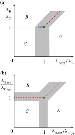
Figure 2: The phase diagram of the Hamiltonian (1) for $p=2$. In panel (a), $\left\{\lambda_{3i-2}\right\}=\left\{\lambda_{A,i}\right\}$ is a set of independent random variables while the remaining couplings $\lambda_{3i-1}=\lambda_{B}$ and $\lambda_{3i}=\lambda_{C}$ are homogeneous. In panel (b), at least two of the coupling constants are independent random variables (see text). The solid red line is a transition line in the Ising universality class of the clean system [$z=1$, see Eq. (9)]. The red dashed lines are transitions in the infinite-randomness universality class [$\psi=1/2$, see Eq. (10)]. The multicritical point (in both cases) is also in the same infinite-randomness universality class. The blue dotted line in panel (a) is a transition line where the universality class is of finite-randomness type ($1<z<\infty)$. The phases have the same nature as the homogeneous case (see Fig. 1) and the shaded regions delimits the associated Griffiths phases where the spectrum gap vanishes.

What are the effects of small coupling $\lambda_{A,i}$? In the clean case, due to triality, small $\lambda_{A}$ cannot shift the location of the critical point $\lambda_{B}=\lambda_{C}$ (see Fig. 1) (see Ref. Fendley, 2019 for another argument). In the disordered case, we numerically show (see Sec. V) that this remains true, i.e., the critical point remains at $\overline{\delta}=\overline{\ln\lambda_{B,i}}-\overline{\ln\lambda_{C,i}}=0$ provided that $\overline{\ln\lambda_{A,i}}<\overline{\ln\lambda_{B,i}}$. Thus, the phase transition lines of the phase diagram, in the random system, are equal to those of the clean system with $\lambda_{A}$, $\lambda_{B}$, and $\lambda_{C}$ replaced by their typical values $\lambda_{A,\text{typ}}$, $\lambda_{B,\text{typ}}$, and $\lambda_{C,\text{typ}}$ as sketched in Fig. 2.

How about the universality classes of the transitions? Here, we consider two cases: two competing (strongest) couplings (a) not generating random mass, and (b) do generating random mass $\delta_{i}$, see Eq. (13).

In case (a) the two strongest couplings are homogeneous ($\lambda_{B,i}=\lambda_{B}$ and $\lambda_{C,i}=\lambda_{C}$) and $\lambda_{A,i}$ is typically much smaller than $\lambda_{B,C}$, the transition is in the universality class of the clean system (Ising) as shown by the solid red line in Fig. 2(a). When approaching the multicritical point, however, the weak disordered couplings $\left\{\lambda_{A,i}\right\}$ become nonperturbative and a line of finite-randomness fixed points emerges (as previously mentioned). The resulting universality class of the transition [blue dotted line in Fig. 2(a)] has critical dynamical exponent $z$ larger than the unity and diverges as the infinite-randomness multicritical point is reached.

In case (b) the two competing couplings generate a random mass ($\overline{\delta^{2}}-\overline{\delta}^{2}\neq 0$). This happens whenever either one or both couplings are independent random variables. The clean (Ising) universality class in unstable since the Harris criterion is violated. The resulting universality class is the one of the random transverse-field Ising chain with activated dynamical scaling (10), and the associated phase boundaries are the dashed lines in the phase diagram of Fig. 2.

III.3 The multicritical point: the case of strong $\lambda_{A,i}$ couplings

What is the change of the clean multicritical point in the presence of disorder? We cannot apply the Harris criterion since the clean correlation length exponent $\nu$ is not known. To answer this question, we develop an appropriate strong-disorder renormalization-group technique (see Sec. IV). Our results strongly indicate that quenched disorder is a relevant perturbation. In addition, we show that the resulting universality class is of infinite-randomness type with activated dynamics (10) and universal tunneling exponent $\psi=\frac{1}{2}$. We have also confirmed these results by numerically studying the finite-size gap of the system (see Sec. V).

III.4 The presence of quantum Griffiths phases

We now inquire about the off-critical properties. Are they affected by quenched disorder? The nature of the phases do not change since disorder on the coupling constants does not break neither a symmetry of the Hamiltonian nor a symmetry of the order-parameter field, i.e., disorder does not couple directly to the order-parameter field in the associated underlying field theory. Thus, the phase diagram has the same phases as the clean one. However, near the transition lines, random mass induces Griffiths phases. In those regions of the phase diagram (shaded areas in Fig. 2), the spectral gap vanishes and the correlations remain short-ranged. The finite-size gap scaling is of power-law type (9) with nonuniversal (i.e., disorder-dependent) effective dynamical exponent $z$.

Here, the Griffiths phases can be understood through the lenses of the so-called rare regions (RRs): large and rare spatial regions in a phase locally different from the bulk. For definiteness, consider the case in which $\lambda_{C,i}=\lambda_{C}$ (i.e., uniform) and $\lambda_{A,i}$’s are distributed between $\lambda_{A,\text{min}}$ and $\lambda_{A,\text{max}}$, with $0<\lambda_{A,\text{min}}<\lambda_{A,\text{max}}$. Evidently the typical value $\lambda_{A,\text{typ}}=\exp(\overline{\ln\lambda_{A}})$ is between $\lambda_{A,\text{min}}$ and $\lambda_{A,\text{max}}$. To start, let us analyze the phase transition between the $A$- ($h^{A}>h^{B,C}$) and $C$-phases ($h^{C}>h^{A,B}$) where we can disregard the weak coupling $\lambda_{B,i}$ (say, for simplicity, that $\max\{\lambda_{B,i}\}<\min\{\lambda_{A,\text{min}},\lambda_{C}\}$). As previously discussed, the transition takes place when $\lambda_{C}=\lambda_{A,\text{typ}}$. When $\lambda_{C}\gg\lambda_{A,\text{max}}$, the system is deep in the homogeneous $C$-phase. Its properties are just the one of the clean systems with the random couplings $\lambda_{A(B),i}$ replaced by their typical value $\lambda_{A(B),\text{typ}}$. Importantly, the spectral gap is finite.

When $\lambda_{A,\text{typ}}<\lambda_{C}<\lambda_{A,\text{max}}$, on the other hand, there are RRs where the local couplings $\lambda_{A,i}$ are typically greater than $\lambda_{C}$. Being locally in the $A$ phase, they endow the system a high $A$-phase susceptibility. The spin in the domain walls between the $A$- and $C$-phases can be arbitrarily weakly coupled and are responsible for the low-lying excitations closing the spectral gap. As neither the bulk nor the RRs are critical, the corresponding correlation length is finite. By duality, an analogous Griffiths phase appears when $\lambda_{A,\text{min}}<\lambda_{C}<\lambda_{A,\text{typ}}$.

Interestingly, there is a simple quantitative argument providing the closing of the spectral gap in the Griffiths phase. Consider a RR of size $L_{\text{RR}}$. The effective interaction between the domain wall spins are thus of order $J_{\text{DW}}\sim e^{-L_{\text{RR}}/\xi_{\text{RR}}}$, where $\xi_{\text{RR}}$ is the corresponding correlation length in that particular RR. For simplicity, we will consider $\xi_{\text{RR}}=\xi$ to be RR-independent (a more precise treatment can be found in Ref. Vojta and Hoyos, 2014). The reason for $J_{\text{DW}}$ being exponentially small is because the RR itself does not harbor Goldstone modes since the symmetry of the Hamiltonian interactions is discrete. The system low-energy density of states $\rho_{\text{DOS}}$ is dominated by the excitations of the weakly coupled domain walls. Ignoring the even weaker coupling to other domain wall spins belonging to other RRs, then $\rho_{\text{DOS}}\left(\omega\right)\sim\int dL_{\text{RR}}w_{\text{RR}}\left(L_{\text{RR}}\right)\delta\left(\omega-J_{\text{DW}}\right)$. Here, we simply sum of all possible RRs weighting their contribution by their existence probability $w_{\text{RR}}\sim e^{-L_{\text{RR}}/\ell}$, with $\ell\propto-1/\ln p$, and $p$ being the probability of $\lambda_{A,i}$ being greater than $\lambda_{C}$. Notice that the probability of finding a RR decreases exponentially with its volume, and $\ell$ is a constant that depends on the distribution’s details of the coupling constants. Consequently, one finds that $\rho_{\text{DOS}}\sim\omega^{-1+1/z}$, with dynamical Griffiths exponent $z=\ell/\xi$. Notice the absence of a gap or a pseudogap in $\rho_{\text{DOS}}$. Actually, there is a divergence in the low-energy density of states when $z>1$ and $\omega\rightarrow 0$. We see that $z$ diverges $\sim 1/\overline{\delta}$ when approaching the transition.

By triality, the resulting Griffiths phases are those sketched in Fig. 2(b) if the $B$-couplings are also randomly distributed between $\lambda_{B,\text{min}}$ and $\lambda_{B,\text{max}}$ ($0<\lambda_{B,\text{min}}<\lambda_{B,\text{max}}$).

Finally, near the multicritical point there are Griffiths phases with RRs locally belonging to, say, either $A$-phase or $B$-phase, while the bulk is in the $C$-phase. A similar feature also appeared in the Griffiths phase of quantum Ashikin-Teller chain (Hrahsheh et al., 2014; Barghathi et al., 2015). In those cases, the effective dynamical exponent $z=\text{max}\{z_{A},z_{B}\}$, where $z_{A(B)}$ is the dynamical exponent provided by the Griffiths singularities of the $A$- ($B$-)RRs.

III.5 The absence of Griffiths phases

If, on the other hand, the $B$-couplings are also homogeneous ($\lambda_{B,i}=\lambda_{B}$), the resulting transition between the $B$- and $C$-phases is the one of the clean transverse-field Ising chain for sufficiently weak $\lambda_{A,\text{max}}$ (as previously discussed). In addition, there is no associated Griffiths phase since there are no RRs ($\lambda_{A,\text{max}}<\lambda_{B}=\lambda_{C}$) as sketched in Fig. 2(a). However, when approaching the multicritical point, RRs in the $A$-phase appear and enhance the low-energy density of states. As a result, the gap closes around the transition. At criticality, those $A$-RRs can even provide a larger dynamical exponent $z$. In that case, the clean critical point is replaced by a line of finite-disorder critical points [dotted boundary line in Fig. 2(a)]. Finally, at the multicritical point, the approximation of weak $A$-couplings completely breaks down and the most general theory contains a random-mass term. Therefore, this critical point is of infinite-randomness type.

IV The strong-disorder renormalization-group method

In this section, we develop a strong-disorder renormalization-group (SDRG) method suitable for studying the long-distance physics of the Hamiltonian (1) for $p=1$ and $2$ and with random coupling constants. It is an energy-based RG method where strongly coupled degrees of freedom are locally decimated out hierarchically. Namely, we search for the strongest coupled local degrees of freedom and freeze them in their local ground state. The couplings between the remaining degrees of freedom are renormalized perturbatively. This procedure becomes more and more accurate if the local energy scales become more and more disordered (broadly distributed). In that case, the perturbative renormalization procedure becomes more accurate after each RG decimation step. This method was originally devised to conventional spin-1/2 models (Ma et al., 1979; Dasgupta and Ma, 1980; Bhatt and Lee, 1982) and later on generalized to many other models. For a review, see Refs. Iglói and Monthus, 2005, 2018.

IV.1 Case $p=1$

IV.1.1 The decimation procedure

To start, let us consider the case $p=1$ in which the model Hamiltonian (1) simplifies to

$$H=-\sum_{j}\lambda_{j}h_{j}=-\sum_{j}\lambda_{j}\sigma_{j}^{x}\sigma_{j+1}^{z}.$$ (14)

For simplicity, we disregard the boundary conditions. Although (14) and the random transverse-field Ising chain are distinct, they share (apart of global degeneracies) the same eigenenergies.

Following the SDRG philosophy, we search for the largest local energy scale $\Omega=\max\left\{\left|\lambda_{j}\right|\right\}$, say $\left|\lambda_{2}\right|$. We then project the Hamiltonian onto the low-energy sector of $H_{0}=-\lambda_{2}h_{2}=-\lambda_{2}\sigma_{2}^{x}\sigma_{3}^{z}$. Denoting $\sigma_{i}^{z}\left|\uparrow_{i}\right\rangle=\left|\uparrow_{i}\right\rangle$, $\sigma_{i}^{z}\left|\downarrow_{i}\right\rangle=-\left|\downarrow_{i}\right\rangle$, $\sigma_{i}^{x}\left|\rightarrow_{i}\right\rangle=\left|\rightarrow_{i}\right\rangle$, and $\sigma_{i}^{x}\left|\leftarrow_{i}\right\rangle=-\left|\leftarrow_{i}\right\rangle$, then the ground-state sector of $H_{0}$ is spanned by $\left|\pm\right\rangle=(\left|\rightarrow_{2},\uparrow_{3}\right\rangle\pm\left|\leftarrow_{2},\downarrow_{3}\right\rangle)/\sqrt{2}$, if $\lambda_{2}>0$, and $\left|\pm\right\rangle=(\left|\rightarrow_{2},\downarrow_{3}\right\rangle\pm\left|\leftarrow_{2},\uparrow_{3}\right\rangle)/\sqrt{2}$, otherwise. As a result, the projection can be interpreted as a replacement of spins $\boldsymbol{\sigma}_{2}$ and $\boldsymbol{\sigma}_{3}$ by an effective spin-1/2 degree of freedom $\tilde{\boldsymbol{\sigma}}$ which is defined by $\tilde{\sigma}^{z}\left|\tilde{\pm}\right\rangle=\pm\left|\tilde{\pm}\right\rangle$. Notice in addition that $\left\langle\pm\left|h_{2}\right|\pm\right\rangle=\left\langle\pm\left|\sigma_{2}^{x}\sigma_{3}^{z}\right|\pm\right\rangle=\text{sign}\left(\lambda_{2}\right)\neq 0$.

The effective system Hamiltonian is obtained by treating $H_{1}=-\lambda_{1}h_{1}-\lambda_{3}h_{3}$ as a perturbation to $H_{0}$. In second order of perturbation theory, we find that

$$\tilde{H}_{1}=-\tilde{\lambda}\tilde{h}+\text{const},\mbox{ with }\tilde{\lambda}=\frac{\lambda_{1}\lambda_{3}}{\Omega}$$ (15)

and $\tilde{h}=\sigma_{1}^{x}\tilde{\sigma}^{z}\sigma_{4}^{z}$. For our purposes, the constant term is harmless and can be disregarded.

Notice that $\tilde{h}$ is now a three-spin interaction. However, since $\tilde{\boldsymbol{\sigma}}$ appears only in $\tilde{h}$, it is a local gauge variable whose role is simply to double the degeneracy of the spectrum. The SDRG decimation procedure (15) can be straightforwardly generalized to operators involving an arbitrary number of “internal” degrees of freedom since the algebra (3) is preserved.

Alternatively, the additional degeneracy induced by the effective internal spin $\tilde{\boldsymbol{\sigma}}$ can be interpreted as if the renormalized chain is, actually, two decoupled new chains. In the first one, $\tilde{\boldsymbol{\sigma}}$ is fixed in state $\left|\tilde{+}\right\rangle$ (the original spins $2$ and $3$ fixed in the ground state $\left|+\right\rangle$ of $H_{0}$) and the corresponding renormalized Hamiltonian is simply $\tilde{H}_{1}=-\tilde{\lambda}\sigma_{1}^{x}\sigma_{4}^{z}$, while in the second one $\tilde{\boldsymbol{\sigma}}$ is fixed at $\left|\tilde{-}\right\rangle$ (the original spins frozen in the state $\left|-\right\rangle$) and $\tilde{H}_{1}=+\tilde{\lambda}\sigma_{1}^{x}\sigma_{4}^{z}$. These two chains have the same spectrum and the subsequent SDRG decimations are identical (apart from the signs of the renormalized couplings which, for our purposes, are not important).

Thus, $\tilde{h}$ can be simplified back to a two-spin interaction at the expense of dealing with two “twins” renormalized chains. The only difference between them being the sign of the renormalized coupling constant $\tilde{\lambda}$.

To use this simplification and keep track of the degeneracies, we are then required to introduce the quantity $g_{\Omega}$. It measures the total number of gauge (extra) spin-1/2 degrees of freedom at the energy scale $\Omega$. Clearly, after each decimation it renormalizes to

$$g_{\Omega}\rightarrow g_{\Omega}+1,$$ (16)

with the initial condition $g_{\Omega_{0}}=0$. The total number of effective degrees of freedom in the chain $N_{\Omega}$ renormalizes to

$$N_{\Omega}\rightarrow N_{\Omega}-2,$$ (17)

with the initial condition $N_{\Omega_{0}}=L$. Notice that $N_{\Omega}+2g_{\Omega}=L$ is a constant throughout the RG flow.

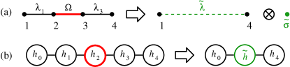
Figure 3: Decimation scheme for the Hamiltonian (1) in the $p=1$ case. In (a), the decimation is sketched in the real space with points and lines representing spin sites and coupling constants, respectively. In (b), the decimation is sketched in the Hamiltonian space with circles representing the local energy operators and the lines connecting anticommuting operators.

In Fig. 3(a) we sketch the decimation procedure (15)–(17). Regarding the local energy scales, the decimation procedure (15) is identical to that of the random spin-1/2 XX chain (Fisher, 1994; Hyman et al., 1996) and that of the random transverse-field Ising chain (Fisher, 1995). This is not a surprise since the free-particle spectra of all these models are the same.

Finally, it is instructive to recast the decimation procedure in the Hamiltonian space as shown in Fig. 3(b). The $j$th circle represents the local energy operator $h_{j}$. A line connecting different circles means that the sharing operators anticommute with each other. Disconnected operators act on different Hilbert spaces and, thus, trivially commute with each other. In the decimation procedure, $h_{2}$ and the “neighboring” operators are replaced by $\tilde{h}$ which anticommutes with the neighboring operators $h_{0}$ and $h_{4}$. The algebra structure is, thus, preserved along the SDRG flow.

IV.1.2 The SDRG flow

Since the SDRG decimation rule (15) is the same as that for the spin-1/2 XX chain, the renormalization-group flow of the coupling constants is already known (Fisher, 1994, 1995; Hyman et al., 1996). Let

$$\delta\equiv\frac{\overline{\ln\lambda_{\text{odd}}}-\overline{\ln\lambda_{\text{even}}}}{\sigma_{\ln\lambda_{\text{odd}}}^{2}+\sigma_{\ln\lambda_{\text{even}}}^{2}},$$ (18)

with $\sigma_{x}^{2}=\overline{x^{2}}-\overline{x}^{2}$ being the variance of $x$. For $\delta\gg 1$, the SDRG flow is towards a stable fixed point in which only the odd couplings are decimated. This implies that only the even couplings are renormalized and, thus, are much smaller than the odd ones. This corresponds to a phase in which $\left|\left\langle h_{2i-1}\right\rangle\right|>\left|\left\langle h_{2i}\right\rangle\right|$. In the spin-1/2 XX chain, this corresponds to the odd-dimer phase where spin singlets are formed over the odd bonds, i.e., $\left|\left\langle\mathbf{S}_{2i-1}\cdot\mathbf{S}_{2i}\right\rangle\right|>\left|\left\langle\mathbf{S}_{2i}\cdot\mathbf{S}_{2i+1}\right\rangle\right|$. The correspondence of this phase in the transverse-field Ising chain is not so straightforward since the XX spin-1/2 chains maps into two independent random transverse-field Ising chains (Fisher, 1994). In the first one, the odd couplings of our model play the role of the transverse fields of the Ising chain. In the second, these roles are exchanged. Thus, the phase $\left|\left\langle h_{2i-1}\right\rangle\right|>\left|\left\langle h_{2i}\right\rangle\right|$ corresponds to the paramagnetic (ferromagnetic) phase in the first (second) quantum Ising chain.

If $0<\delta\ll 1$, the system is in the associated Griffiths phase. Typically, $\left|\left\langle h_{\text{odd}}\right\rangle\right|>\left|\left\langle h_{\text{even}}\right\rangle\right|$, but there are some “defects” inside which $\left|\left\langle h_{\text{odd}}\right\rangle\right|<\left|\left\langle h_{\text{even}}\right\rangle\right|$. These defects form the rare regions discussed in Sec III. Surrounding a rare region, there are two (domain-wall) spins weakly coupled. As a result of their weak coupling, the typical and mean values of the finite-size gap vanish $\sim L^{-z}$ [Eq. (9)], which defines an off-critical dynamical (Griffiths) exponent $z$. As the critical point is approached, this exponent diverges as $z\sim\left|\delta\right|^{-1}$.

We now further discuss on the effects of the RRs in the Griffiths phase through the lenses of the SDRG method. Recall that, in the transverse-field Ising chain, the origin of the gapless modes in, say, the paramagnetic phase is due the RRs which are locally in the ferromagnetic phase and fluctuate between the two ferromagnetic states. As this is a coherent tunneling process involving many spins, the associated relaxation time increasing exponentially with the RR’s volume. In the XX spin-1/2 chain, these RRs correspond to patches which are locally in the even-dimer phase while the bulk is in the odd-dimer phase. The two domain walls delimiting a RR are, in zeroth order of approximation, simply free (unpaired) spins. To lowest nonvanishing order in perturbation theory, these spins (say, at sites $1$ and $\ell$) actually interact via an effective coupling constant equal to $\tilde{\lambda}_{\ell}=\lambda_{1}\lambda_{3}\dots\lambda_{\ell-1}/\lambda_{2}\lambda_{4}\dots\lambda_{\ell-2}$ [which could also be obtained by a successive iteration of Eq. (15)]. Thus, the gap of a finite chain is simply the excitation energy of the weakest coupled spins in these domain walls: $\min\{|\tilde{\lambda}_{\ell}|\}$. Notice that, as expected, $\tilde{\lambda}_{\ell}$ vanishes exponentially with the RR size implying an exponentially large relaxation time. An analogous physical picture appears in our model. For simplicity, consider a compact RR in which the local even couplings $\lambda_{2},\,\lambda_{4},\,\dots,\,\lambda_{\ell-2}$ ($\ell$ even) are greater than the local odd couplings $\lambda_{1},\,\lambda_{3},\,\dots,\,\lambda_{\ell-1}$. In that case, after decimating the even operators $h_{2i}$ in that RR, an effective operator linking spins $1$ and $\ell$ appear $\tilde{h}_{1}=-\tilde{\lambda}_{\ell}\sigma_{1}^{x}\sigma_{\ell}^{z}$ with $\tilde{\lambda}_{\ell}=\lambda_{1}\lambda_{3}\dots\lambda_{\ell-1}/\lambda_{2}\lambda_{4}\dots\lambda_{\ell-2}$ (disregarding an unimportant sign). Thus, $\left\langle h_{2}\right\rangle=\left\langle h_{4}\right\rangle=\dots=\left\langle h_{2\ell-2}\right\rangle=\pm 1$ and a longer correlation between spins $1$ and $\ell$ develop, $\left\langle\sigma_{1}^{x}\sigma_{\ell}^{z}\right\rangle\neq 0$. Consequently, a low-energy mode arises with excitation energy of order $\tilde{\lambda}$. Evidently, by duality, there are analogous conventional and Griffiths phases for $\delta<0$.

At criticality $\delta=0$, the fixed point is universal in the sense that critical exponents do not depend on the details of the disorder distributions. For instance, the finite-size gap distribution for sufficiently large systems is (Fisher and Young, 1998)

$${\cal P}_{\text{SDRG}}\left(\eta\right) = \frac{4}{\sqrt{\pi}}\sum_{k=0}^{\infty}\left(-1\right)^{k}\left(k+\frac{1}{2}\right)e^{-\eta^{2}\left(k+\frac{1}{2}\right)^{2}},$$ (19)

$$= \frac{4\pi}{\eta^{3}}\sum_{k=0}^{\infty}\left(-1\right)^{k}\left(k+\frac{1}{2}\right)e^{-\pi^{2}\left(k+\frac{1}{2}\right)^{2}/\eta^{2}},\quad$$

where

$$\eta=\frac{\ln\left(2\Omega_{0}/\Delta\right)}{\sigma_{0}\left(L/2\right)^{\psi}},$$ (20)

$\sigma_{0}=\sqrt{\frac{1}{2}\sigma_{\ln\lambda_{\text{odd}}}^{2}+\frac{1}{2}\sigma_{\ln\lambda_{\text{even}}}^{2}}$, $\Omega_{0}$ is the maximum value of $\lambda$ in the bare system, $\Delta$ is the finite-size gap, and $\psi=1/2$ is the universal tunneling exponent. The distribution ${\cal P}_{\text{SDRG}}$ is $L$ independent for $L\gg\gamma_{D}^{-1}=\pi/8\sigma_{\ln\lambda}^{2}$, the inverse of the Lyapunov exponent (Mard et al., 2014) which plays the role of a clean-dirty crossover length (Laflorencie et al., 2004; Wada and Hoyos, 2022). The relation between length and energy scales follow from the scaling variable in Eq. (20), from which follows the activated dynamical scaling $\overline{\ln\Delta}\sim-L^{\psi}$ in Eq. (10).

IV.1.3 Thermodynamics

The thermodynamic observables follow straightforwardly. For instance, the low-temperature entropy is simply $S\sim\frac{1}{L}\left(N_{T}+g_{T}\right)\ln 2$, which simply counts the total number of active (undecimated) spins at the energy scale $\Omega=T$. The reasoning is the following (Bhatt and Lee, 1982). At low temperatures $T\ll\Omega_{0}$, the distribution of effective coupling constants is singular and, thus, the majority of the couplings are much smaller than the maximum energy scale $\Omega=T$. In sum, the active spins are essentially free. At criticality ($\delta=0$), $N_{\Omega}\approx L/\left(1+\ln\left(\Omega_{0}/\Omega\right)/\sigma_{\ln\lambda}^{2}\right)^{1/\psi}$ (Iglói et al., 2001; Hoyos et al., 2007b) and $g_{\Omega}=\frac{1}{2}\left(L-N_{\Omega}\right)$. Then,

$$S=\frac{1}{2}\left(1+\left(\frac{\sigma_{\ln\lambda}^{2}}{\ln\left(\frac{\Omega_{0}}{T}\right)}\right)^{1/\psi}\right)\ln 2.$$ (21)

Notice the residual zero-temperature entropy coming from the exponentially large ground-state degeneracy.

The specific heat follows from $C=T\partial S/\partial T$. In the low-temperature limit,

$$C\sim\ln^{-\left(1+1/\psi\right)}\left(\Omega_{0}/T\right),$$ (22)

which is similar to that of the random spin-1/2 XX chain.

IV.1.4 Ground-state degeneracy and the spectrum of other models

It is interesting to further explore the connection between the $p=1$ model, the spin-1/2 XX chain, and the transverse-field Ising chain in view of the SDRG decimation procedure.

Within the SDRG framework, one can obtain the whole spectrum of the transverse-field Ising chain in the following way (Pekker et al., 2014). When performing the decimating procedure, one can either search for the ground state (and then project onto ground state of the local Hamiltonian) or, alternatively, search for the excited states (and then project onto the excited state of the local Hamiltonian). If one projects onto the excited states, the effective coupling of field pics up a different sign but the magnitude is the same [see Eq. (15)]. However, for decimation purposes, all remains the same as the sign is irrelevant. Performing the decimation for all possibilities of low and excited states, one constructs the entire spectrum of the Ising chain: $2^{L/2}$ states in total. (Recall that the associated Ising chain has half of the sites, but the same number of operators in the Hamiltonian.) Notice that this is equivalent to consider two “twins” renormalized chains as previously outlined. Thus, all ground states of the $p=1$ model are equivalent to the entire spectrum of the transverse-field Ising chain.

The connection to the XX model is alike. Here, the local Hamiltonian has $3$ energy levels: one corresponds to the spin-$0$ singlet state, another to the zero-magnetization spin-$1$ triplet state, and the remaining one is doubly degenerate corresponding to the $\pm 1$-magnetization spin-$1$ states. If one disregards the doubly degenerate $\pm 1$-magnetization states, the decimation procedure recovers that of the Ising chain. Thus, the many ground-states of the $p=1$ model corresponds to a small fraction of the states in the spectrum of the XX spin-1/2 chain.

We now inquire about the spectrum of the $p=1$ chain. When projecting the system onto to local excited states, the only difference with respect to projecting onto the local ground state is a sign picked up by the effective energy scales and a flip of one of the spins. Thus, the entire spectrum can be easily related to the states in the ground-state manifold. There will be $2^{\frac{L}{2}}$ states each of which is $2^{\frac{L}{2}}$ degenerate. Precisely, all states can be represented by

$$\otimes_{j=1}^{L/2}\left|\phi_{j}\right\rangle,$$ (23)

where $\left|\phi_{j}\right\rangle$ is either $\left|\phi_{j,+}\right\rangle=(\left|\rightarrow_{j_{1}},\uparrow_{j_{2}}\right\rangle\pm\left|\leftarrow_{j_{1}},\downarrow_{j_{2}}\right\rangle)/\sqrt{2}$ or $\left|\phi_{j,-}\right\rangle=(\left|\rightarrow_{j_{1}},\downarrow_{j_{2}}\right\rangle\pm\left|\leftarrow_{j_{1}},\uparrow_{j_{2}}\right\rangle)/\sqrt{2}$. Here, $\left\{j_{1},j_{2}\right\}$ is the pair of spin sites decimated together in the $j$th decimation which is the same pair for all states. The precise state $\left|\phi_{j}\right\rangle$ (if $\left|\phi_{j,+}\right\rangle$ or $\left|\phi_{j,-}\right\rangle$ and with the $+$ or $-$ sign) depends on the sign of coupling constant and on whether the projection was made into the local ground or excited states. All of these, are determined by the history of decimation procedure.

IV.1.5 Spin-spin correlations

In the SDRG approach, any of the $2^{L/2}$ ground states of $H_{0}$ is a simply product state as specified in (23). In that case, the spins in the $j$th pair are strongly correlated and dominates the average value of the spin-spin correlation. The probability that a pair of length $r=j_{2}-j_{1}$ is formed along the SDRG flow is proportional to $r^{-2}$ for sufficiently large $r$ (Fisher, 1994; Hoyos et al., 2007b). Hence, the mean correlation function decays only algebraically,

$$\overline{\left|\left\langle\sigma_{i}^{x}\sigma_{i+r}^{z}\right\rangle\right|}\sim r^{-\eta},$$ (24)

with universal exponent $\eta=2$. (Here, $\overline{\cdots}$ denotes the disorder average.) The typical value of the correlation, on the other hand, decays stretched exponentially fast (Fisher, 1994),

$$\overline{\ln\left|\left\langle\sigma_{i}^{x}\sigma_{i+r}^{z}\right\rangle\right|}\sim-r^{\psi}.$$ (25)

The distribution of the values of the correlation function is also known. For that, we refer the reader to Refs. Getelina and Hoyos, 2020; Wada and Hoyos, 2022.

The off-critical ($\delta\neq 0$) correlations are also known (Fisher, 1994, 1995; Hoyos et al., 2011). They decay exponentially faster $\sim e^{-r/\xi}$ with a diverging correlation length

$$\xi\sim\delta^{-\nu},$$ (26)

where $\nu=2$ for the mean correlations and $\nu=1$ for the typical correlations.

Interestingly, all those results apply for any state as well provided that only the magnitude of the correlations are concerned.

IV.2 Case $p=2$

IV.2.1 The usual SDRG method

We now derive the SDRG decimation rules for the Hamiltonian (1) with $p=2$.

Following the usual SDRG receipt, we treat $H_{1}=-\lambda_{3}h_{3}-\lambda_{4}h_{4}-\lambda_{6}h_{6}-\lambda_{7}h_{7}$ (where $h_{j}=\sigma_{j}^{x}\sigma_{j+1}^{z}\sigma_{j+2}^{z}$) as a perturbation to $H_{0}=-\lambda_{5}h_{5}$. (We are assuming that the energy cutoff $\Omega=\left|\lambda_{5}\right|$.) Up to second order in perturbation theory, the renormalized Hamiltonian is $\tilde{H}_{1}=P_{0}H_{1}^{2}P_{0}/\left(-2\left|\lambda_{5}\right|\right)$, where $P_{0}$ is the projector onto the ground state of $H_{0}$. The direct terms in the square of $H_{1}$ are unimportant constants since $h_{i}^{2}=1$. The cross terms are proportional to the anticommutators $\left\{h_{i},h_{j}\right\}$. Thus, many of those vanish because of the algebra (3). The surviving ones are those which commute with each other. Thus, $\tilde{H}_{1}$ simplifies to $\tilde{H}_{1}=-\tilde{\lambda}_{C}\tilde{h}_{C}-\tilde{\lambda}_{AC}\tilde{h}_{AC}-\tilde{\lambda}_{A}\tilde{h}_{A}$ where the operators are

$$\tilde{h}_{C} = P_{0}h_{3}h_{6}P_{0}=\sigma_{3}^{x}\sigma_{4}^{z}\tilde{\sigma}^{x}\tilde{\tau}^{z}\sigma_{8}^{z},$$

$$\tilde{h}_{AC} = P_{0}h_{3}h_{7}P_{0}=\sigma_{3}^{x}\sigma_{4}^{z}\tilde{\sigma}^{x}\tilde{\tau}^{x}\sigma_{8}^{z}\sigma_{9}^{z},$$ (27)

$$\tilde{h}_{A} = P_{0}h_{4}h_{7}P_{0}=-\sigma_{4}^{x}\tilde{\sigma}^{y}\tilde{\tau}^{y}\sigma_{8}^{z}\sigma_{9}^{z},$$

and the renormalized couplings are

$$\tilde{\lambda}_{C}=\frac{\lambda_{3}\lambda_{6}}{\Omega},\ \tilde{\lambda}_{AC}=\frac{\lambda_{3}\lambda_{7}}{\Omega},\mbox{ and }\tilde{\lambda}_{A}=\frac{\lambda_{4}\lambda_{7}}{\Omega}.$$ (28)

Here, the effective degrees of freedom $\tilde{\boldsymbol{\sigma}}$ and $\tilde{\boldsymbol{\tau}}$ span the ground-state subspace $\{\left|\rightarrow\uparrow\uparrow\right\rangle,$ $\left|\rightarrow\downarrow\downarrow\right\rangle,$ $\left|\leftarrow\downarrow\uparrow\right\rangle,$ $\left|\leftarrow\uparrow\downarrow\right\rangle\}$ for $\lambda_{5}>0,$ otherwise the set of states is $\{\left|\leftarrow\uparrow\uparrow\right\rangle,$ $\left|\leftarrow\downarrow\downarrow\right\rangle,$ $\left|\rightarrow\downarrow\uparrow\right\rangle,$ $\left|\rightarrow\uparrow\downarrow\right\rangle\}$. These states are recognized as $\{\left|\uparrow,\uparrow\right\rangle,$ $\left|\uparrow,\downarrow\right\rangle,$ $\left|\downarrow,\uparrow\right\rangle,$ $\left|\uparrow,\uparrow\right\rangle\}$ in the $\tilde{\sigma}^{z}\otimes\tilde{\tau}^{z}$-basis.

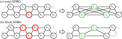
Figure 4: Strong-disorder RG decimation scheme for the Hamiltonian (1) in the $p=2$ case. The decimation is depicted in the Hamiltonian space analogous to Fig. 3(b) where circles represent the local energy operators and lines connect operators which anticommute. In (a), the SDRG method is implemented in its simpler form (usual SDRG) where a newly generated operator $\tilde{h}_{AB}$ disrupts the algebra (3). In (b), the SDRG method is implemented in a slightly more general fashion (block SDRG) which preserves the algebra (3) in the renormalized chain .

The decimation procedure (27) and (28) is represented in the Hamiltonian space in Fig. 4(a). Unlike the $p=1$ case [see Fig. 3(b)], the structure of the anticommuting algebra (3) of the original Hamiltonian is not preserved and new operators (involving $\sigma^{y}$) appear.

IV.2.2 The block SDRG method

The arising of the new operator $\tilde{h}_{AC}$ in (27) hinders the practical implementation of the method. First, it prevents us from projecting the renormalized system onto the ground states of the new effective spin operators $\tilde{\boldsymbol{\sigma}}$ and $\tilde{\boldsymbol{\tau}}$ as in the $p=1$ case. Second, and more importantly, it requires a generalization of the SDRG procedure to take into account these new operators. While this is possible and cumbersome, we found, surprisingly, a quite simpler route guided by the algebra of the energy-density operators (3). We generalize the “usual” SDRG approach above reported to (in the lack of a better therminology) a “block” SDRG approach. In the latter, we consider a larger unperturbed Hamiltonian (and thus, a larger Hilbert space) when performing the decimation procedure (see details in Appendix A). The size of the block is the maximum number of operators which anticommute among themselves.

When decimating the largest local energy scale $\Omega=\left|\lambda_{5}\right|$, instead of considering $H_{0}=-\lambda_{5}h_{5}$ (which is a $B$-type operator), we consider a larger block involving the $A$- and $C$-type “nearest-neighbor” operators, i.e., $H_{0}=-\lambda_{4}h_{4}-\lambda_{5}h_{5}-\lambda_{6}h_{6}$. This is the largest block which encompass $h_{5}$ and still have only two energy levels (as $h_{5}$), i.e., the eigenenergies of $H_{0}$ are $\pm\sqrt{\lambda_{4}^{2}+\lambda_{5}^{2}+\lambda_{6}^{2}}$. Then, we project the $H-H_{0}$ on the ground-state subspace of $H_{0}$. The degeneracy of the ground state is $2^{4}$ and, thus, can be spanned by four effective spin-1/2 degrees of freedom $\tilde{\boldsymbol{\sigma}}_{a}$, $\tilde{\boldsymbol{\sigma}}_{b}$, $\tilde{\boldsymbol{\sigma}}_{c}$, and $\tilde{\boldsymbol{\sigma}}_{d}$. In practice, we have to project $\lambda_{2}h_{2}$, $\lambda_{3}h_{3}$, $\lambda_{7}h_{7}$ and $\lambda_{8}h_{8}$. The result is that, in the regime $\left|\lambda_{5}\right|\gg\left|\lambda_{4,6}\right|$, the renormalized operators are

$$\tilde{h}_{2}=\sigma_{2}^{x}\sigma_{3}^{z}\tilde{\sigma}_{a}^{z}\left(\sin\theta\tilde{\sigma}_{b}^{x}\tilde{\sigma}_{d}^{z}+\cos\theta\tilde{\sigma}_{b}^{z}\right)\tilde{\sigma}_{c}^{z},$$ (29)

where

$$\cos\theta=\frac{-\text{sign}\left(\lambda_{5}\right)\left|\lambda_{4}\right|}{\sqrt{\lambda_{4}^{2}+\lambda_{6}^{2}}}\mbox{ and }\sin\theta=\frac{\lambda_{6}}{\sqrt{\lambda_{4}^{2}+\lambda_{6}^{2}}},$$ (30)

$$\tilde{h}_{8}=-\text{sign}\left(\lambda_{5}\right)\left(\cos\theta\tilde{\sigma}_{d}^{x}+\sin\theta\tilde{\sigma}_{b}^{y}\tilde{\sigma}_{d}^{y}\right)\sigma_{9}^{z}\sigma_{10}^{z},$$ (31)

$$\tilde{h}_{3}=\sigma_{3}^{x}\tilde{\sigma}_{a}^{y}\tilde{\sigma}_{b}^{y}\tilde{\sigma}_{c}^{z}\tilde{\sigma}_{d}^{z},\mbox{ and }\tilde{h}_{7}=\tilde{\sigma}_{c}^{x}\tilde{\sigma}_{d}^{z}\sigma_{9}^{z}.$$ (32)

The corresponding renormalized coupling constants are $\tilde{\lambda}_{2}=\lambda_{2}$, $\tilde{\lambda}_{8}=\lambda_{8}$,

$$\tilde{\lambda}_{3}=-\text{sign}\left(\lambda_{4}\right)\frac{\lambda_{3}\lambda_{6}}{\Omega},\mbox{ and }\tilde{\lambda}_{7}=\frac{\left|\lambda_{4}\right|\lambda_{7}}{\Omega}.$$ (33)

Surprisingly, the renormalized operators are different in character from those in Eq. (27). Interestingly, they preserve the algebra structure (3) of the original system as depicted in Fig. 4(b) if we identify $\tilde{h}_{2}\rightarrow h_{2}$, $\tilde{h}_{3}\rightarrow\tilde{h}_{C}$, $\tilde{h}_{7}\rightarrow\tilde{h}_{A}$, and $\tilde{h}_{8}\rightarrow h_{8}$. Furthermore, the “hybrid” operator $\tilde{h}_{AC}$ [generated from the usual SDRG approach, see Fig. 4(a)] is not generated in the block SDRG approach [see Fig. 4(b)]. Instead, there are only “pure” operators except for the $BC$-type operator in (29) and the $AB$-type operator in (31). This is very convenient because they can be neglected at strong-disorder fixed points (corresponding to situations near and at the dashed transitions in Fig. 2). The reasoning is the following. Since the effective disorder at and near the transition is very large (which we show a posteriori), very likely either $\left|\lambda_{4}\right|\gg\left|\lambda_{6}\right|$ or the $\left|\lambda_{4}\right|\ll\left|\lambda_{6}\right|$. In the former case, $\sin\theta\approx 0$ in Eq. (30), and, thus, the hybrid type operators can be neglected. The renormalized $B$-type operators then simplify to $\tilde{h}_{2}=-\text{sign}\left(\lambda_{5}\right)\sigma_{2}^{x}\sigma_{3}^{z}\tilde{\sigma}_{a}^{z}\tilde{\sigma}_{b}^{z}\tilde{\sigma}_{c}^{z}$, $\tilde{h}_{8}=\tilde{\sigma}_{d}^{x}\sigma_{9}^{z}\sigma_{10}^{z}$. Taking $\sin\theta=1-\cos\theta=0$ and noticing that the new effective spin-1/2 degrees of freedom $\tilde{\boldsymbol{\sigma}}_{a}$ and $\tilde{\boldsymbol{\sigma}}_{b}$ appear only in combinations that commute with each other ($\tilde{\sigma}_{a}^{z}\tilde{\sigma}_{b}^{z}$ in $\tilde{h}_{2}$ and $\tilde{\sigma}_{a}^{y}\tilde{\sigma}_{b}^{y}$ in $\tilde{h}_{3}$), we can project the resulting renormalized Hamiltonian in the common eigenstates of $\tilde{\sigma}_{a}^{z}\tilde{\sigma}_{b}^{z}$ and $\tilde{\sigma}_{a}^{y}\tilde{\sigma}_{b}^{y}$. As a result, we have four “twins” renormalized systems. They are

$$\tilde{H}_{1}=\pm\lambda_{2}h_{2}\pm\tilde{\lambda}_{C}\tilde{h}_{C}-\tilde{\lambda}_{A}\tilde{h}_{A}-\lambda_{8}h_{8},$$ (34)

where $h_{2}=\sigma_{2}^{x}\sigma_{3}^{z}\tilde{\sigma}_{c}^{z}$, $\tilde{h}_{C}=\sigma_{3}^{x}\tilde{\sigma}_{c}^{z}\tilde{\sigma}_{d}^{z}$, $\tilde{h}_{A}=\tilde{\sigma}_{c}^{x}\tilde{\sigma}_{d}^{z}\sigma_{9}^{z}$, $h_{8}=\tilde{\sigma}_{d}^{x}\sigma_{9}^{z}\sigma_{10}^{z}$,

$$\tilde{\lambda}_{C}=\frac{\lambda_{3}\lambda_{6}}{\Omega},\mbox{ and $\tilde{\lambda}_{A}$=$\frac{\left|\lambda_{4}\right|\lambda_{7}}{\Omega}$.}$$ (35)

The decimation procedure (34) and (35) is schematically depicted in Fig. 4(b). By symmetry, an analogous decimation procedure is obtained in the case $\left|\lambda_{4}\right|\ll\left|\lambda_{6}\right|$, with the exchanges $\lambda_{2}\leftrightharpoons\lambda_{8}$ and $\tilde{\lambda}_{A}\leftrightharpoons\tilde{\lambda}_{C}$, which is obtained after a convenient change in the definition of the effective operators $\tilde{\boldsymbol{\sigma}}_{a}$, $\tilde{\boldsymbol{\sigma}}_{b}$, $\tilde{\boldsymbol{\sigma}}_{c}$, and $\tilde{\boldsymbol{\sigma}}_{d}$.

The decimation procedure (34) and (35) [see Fig. 4(b)] is very convenient. It preserves the algebra structure (3) and the operators of the original Hamiltonian $\tilde{h}_{i}=\sigma_{i}^{x}\sigma_{i+1}^{z}\sigma_{i+2}^{z}$. This procedure is a straightforward generalization of the decimation procedure of the $p=1$ case in the following sense. For $p=1$, a decimation of an $A$-type coupling implies the renormalization of the neighboring $B$-type couplings and vice versa [see Eq. (15)]. For $p=2$, due to triality, the decimation of a $B$-type operator implies the renormalization of the neighboring $A$- and $C$-type couplings [see Eq. (35)].

IV.2.3 On the equivalence between the usual and the block SDRG approaches

In the regime $\left|\lambda_{5}\right|\gg\left|\lambda_{4,3}\right|$, there should be no difference between the usual and block SDRG approaches as the ground state of the block $H_{0}=-\lambda_{4}h_{4}-\lambda_{5}h_{5}-\lambda_{6}h_{6}$ is simply that of the local $H_{0}=-\lambda_{5}h_{5}$ furnished with trivial degeneracies. It is somewhat surprising that seemingly fundamentally different decimation procedures arise from these approaches. Thus, we inquire whether these two decimating procedures are really different.

In Ref. Hoyos and Miranda, 2004a the SDRG method was carried out in the antiferromagnetic Heisenberg model in a zigzag and two-leg ladder geometries. In both cases, it was shown that, in the early stages of the SDRG flow, further neighbors interactions arise, just like what was found in the usual SDRG decimation [see Fig. 4(a)]. However, in the final stages of the SDRG flow, the renormalized geometry of the system always converged to a chain geometry. (Evidently, one had to disregard exceedingly small couplings that were generated along the flow.) This may be a general feature of quasi-one-dimensional critical or near-critical systems. The low-energy long-wavelength effective theory is that of a chain. Technically, couplings of “long” operators that connect exceedingly distant spins arise after many renormalizations and, thus, are typically much smaller than those of “shorter” operators.

In sum, the longer range character of the new hybrid operator $\tilde{h}_{AC}$ in the usual SDRG approach may be an irrelevant “operator” which vanishes in the latter stages of the SDRG flow. In the block SDRG approach, the new hybrid operators $\tilde{h}_{AB}$ and $\tilde{h}_{BC}$ could be clearly determined as irrelevant ones near and at criticality, where the flow is towards strong disorder, a self-consistent assumption that we have yet to prove. Therefore, it is plausible that $\tilde{h}_{AC}$ in the usual SDRG approach can be neglected by the same reasons. In that case, both the usual and block SDRG approaches are equivalent near and at criticality. This is a fundamental feature of the renormalization-group philosophy. Details on defining the coarse-grained operators should not matter in the long-wavelength regime.

IV.2.4 SDRG flow corresponding to conventional phases

Having derivied the SDRG decimation rules, we now analyze the flow of the coupling constants.

Let us start by analyzing the simpler case corresponding to flow towards the gapped phases. In this case, one of the coupling constants, say, of $C$-type, is always greater than the others. Precisely, $\min\left\{\lambda_{3i}\right\}>\max\left\{\lambda_{3i-1},\lambda_{3i-2}\right\}$. In that case, notice that only the bare $h_{3i}$ operators are decimated. Therefore, the corresponding fixed point is noncritical and, thus, represents a phase: the $h^{C}>h^{A,B}$ conventional phase in Fig. 2. Notice that both the usual and the block SDRG can be applied here since only the original $h_{3i}$ operators are decimated. Thus, in the SDRG framework, the spectrum gap is simply $\Delta=2\min\left\{\lambda_{3i}\right\}$.

Evidently, by triality, there are additional two phases in which $h^{A}>h^{B,C}$ and $h^{B}>h^{A,C}$ as shown in Fig. 2. Finally, we call attention to the fact that, in the SDRG framework, these phases exist because a decimation of $h_{i}$, renormalizes the neighboring interactions $h_{j}$ with $\left|j-i\right|\leq p=2$. Thus, for a generic value of $p$ in the Hamiltonian (1), we expect, at least, $p+1$ different phases.

IV.2.5 SDRG flow corresponding to conventional Griffiths phases and phase transitions between two phases.

First, we analyze the case in which at least two of the three types of couplings are random, i.e., the SDRG flow associated with the transitions and Griffiths phases shown in Fig. 2(b) away from the multicritical point.

Let us consider the case in which $\max\left\{\lambda_{3i-2}\right\}<\min\left\{\lambda_{3i-1},\lambda_{3i}\right\}$. In this case, the SDRG flow is dictated only by the competition between $\left\{\lambda_{3i}\right\}$ and $\left\{\lambda_{3i-1}\right\}$ as the $A$-type couplings will never be decimated. Thus, we can simply drop the $\lambda_{A}$’s in the decimation procedure (34) and (35) as the distribution $P_{A}$ renormalizes to an extremely singular one. In that case, the zigzag-chain geometry of the renormalized system becomes that of a single chain. Therefore, the flow is simply that of the case $p=1$.

To analyze it, we simply generalize the distance from criticality Eq. (18) to

$$\delta_{BC}\equiv\frac{\overline{\ln\lambda_{3i}}-\overline{\ln\lambda_{3i-1}}}{\sigma_{\ln\lambda_{B}}^{2}+\sigma_{\ln\lambda_{C}}^{2}}.$$ (36)

From here, all energy-related results from the $p=1$ case follows straightforwardly. The transition is governed by an infinite-randomness critical point and happens for $\delta_{BC}=0$. The gap distribution is that of Eq. (19) with the scaling variable (20) redefined as

$$\eta=\frac{\ln\left(2\Omega_{0}/\Delta\right)}{\sigma_{0}\left(L/3\right)^{\psi}}.$$ (37)

This redefinition is due to the fact that the total number of decimations in the $p=1$ case is $L/2$ while it is $L/3$ for the $p=2$ case. Thus, $L/2$ in the $p=1$ case translates to $L/3$ in the $p=2$ case.

In addition, there are associated Griffiths phases for $\left|\delta_{BC}\right|\ll 1$. The off-critical dynamical exponent $z$ diverges as $z\sim\left|\delta_{BC}\right|^{-1}$ when it approaches criticality. The nature of the low-energy modes are also associated with domain wall spins surrounding a rare region, just like for $p=1$.

By triality, there are other two boundary transitions for $\delta_{AB}=0$ and $\delta_{AC}=0$. These boundaries and the Griffiths phases are shown in Fig. 2 as dashed lines and shaded regions, respectively. The SDRG results here reported, thus, put the heuristic arguments of Sec. III in solid grounds.

Now we analyze the case in which the two competing (strongest) couplings are uniform, i.e., $\lambda_{B,i}=\lambda_{B}$, $\lambda_{C,i}=\lambda_{C}$, and $\lambda_{A,i}$ random with $\lambda_{A,\text{typ}}<\lambda_{B,C}$. This corresponds to the region in the phase diagram of Fig. 2(a) surrounding the clean and finite-randomness transition but sufficiently far from the multicritical point.

When $\max\left\{\lambda_{A,i}\right\}<\lambda_{B,C}$, the SDRG method does not need to be applied since weak $\lambda_{A}$ coupling is irrelevant. The transition at $\lambda_{B}=\lambda_{C}$ is in the clean Ising universality class, and the spectral gap vanishes only at criticality.

When $\lambda_{A,\text{typ}}<\lambda_{B}<\lambda_{C}<\max\left\{\lambda_{A,i}\right\}$, the system in the Griffiths $C$-phase with high $A$-susceptibility as in the generic case discussed above. (Analogously for $\lambda_{A,\text{typ}}<\lambda_{C}<\lambda_{B}<\max\left\{\lambda_{A,i}\right\}$.)

Finally, we discuss the interesting case when $\lambda_{A,\text{typ}}<\lambda_{B}=\lambda_{C}<\max\left\{\lambda_{A,i}\right\}$. The system is globally critical between $B$- and $C$-phases but there are rare regions locally in the $A$-phase. What are their effects? Applying the block-SDRG decimation procedure, we simply decimate $A$-operators in the first stages of the flow. After decimating all $A$-operators with $\lambda_{B}=\lambda_{C}<\lambda_{A,i}<\max\left\{\lambda_{A,i}\right\}$, we can simply ignore the remaining $A$-operators since they would be surrounded by locally stronger $B$- and $C$-operators. The effective chain is, thus, that with $B$- and $C$-operators only. However, the effective coupling constants are not uniform. Interestingly, notice that the effective couplings obey the condition $\tilde{\lambda}_{B,i}=\tilde{\lambda}_{C,i}$. The precise condition for the absence of random distances from criticality (random mass) discussed in Sec. III.1.2. When the $A$-rare regions are small, the effective couplings $\tilde{\lambda}_{B,C,i}$ are weakly renormalized and their effective disorder (variance of their distribution) is weak. As a result, the clean critical behavior is stable. However, when approaching the multicritical point we expect the renormalization of $\tilde{\lambda}_{B,C,i}$ to become more and more relevant. This means that their effective disorder increases to the point where the clean critical behavior is destabilized. The resulting phase transition is thus of finite-randomness type with nonuniversal critical exponent $z$. This result should be valid up to the multicritical point where $z$ reaches its maximum value. Interesting, $z$ is formally infinity in the other transition lines meeting at the multicritical point.

We end this section by noticing that the above results straightforwardly generalizes to any value of $p$.

IV.2.6 The SDRG flow at the multicritical point

Finally, we deal with the case in which all couplings compete.

At first glance, one could think in analyzing the flow equations for the distributions $P_{A}$, $P_{B}$, and $P_{C}$ analytically. The flow equation for $P_{A}$ is (see Appendix B)

$$-\frac{\partial P_{A}}{\partial\Omega}=P_{A}\left(\Omega\right)P_{A}-\left(P_{B}\left(\Omega\right)+P_{C}\left(\Omega\right)\right)\left(P_{A}-P_{A}\otimes P_{A}\right),$$ (38)

where $P_{X}=P_{X}\left(\lambda;\Omega\right)$, $P_{X}\left(\Omega\right)=P_{X}\left(\Omega;\Omega\right)$, and

$$P_{X}\otimes P_{X}=\int d\lambda_{1}d\lambda_{4}P_{X}\left(\lambda_{1};\Omega\right)P_{X}\left(\lambda_{4};\Omega\right)\delta\left(\lambda-\frac{\lambda_{1}\lambda_{4}}{\Omega}\right).$$ (39)

By triality, the flow equations for $P_{B}$ and $P_{C}$ follow from exchanging the labels accordingly. The last term on the r.h.s. of (38) implements the renormalization of the $A$-type coupling [$\tilde{\lambda}_{A}$ in Eq. (35), and we are considering only the magnitude of the coupling constants] when a $B$- or $C$-type coupling is decimated. The remaining terms ensure that $P_{A}$ remains normalized when the cutoff energy scale $\Omega$ is changed. As shown in App. B, the critical point (where $P_{A}=P_{B}=P_{C}$) of the flow equation (38) is of infinite-randomness type [see Eq. (56)] and is related to a different universal tunneling exponent $\psi=\frac{2}{3}$ which is greater than that $\psi=\frac{1}{2}$ of the case $p=1$. A larger tunneling exponent means larger effective disorder as the typical value of the finite-size gap is even smaller [see Eq. (37)]. This sounds intuitive since two coupling constants are renormalized in each decimation instead of one renormalization per decimation as happens in the $p=1$ case.

Although this gives us a prescription to find a new universality class beyond that of the permutation-symmetric universality class (where $\psi=1/N$, with $N$ being an integer (Damle and Huse, 2002; Hoyos and Miranda, 2004b; Fidkowski et al., 2009; Quito et al., 2020, 2019)), the analytical analysis of this problem is not correct. The flow equation (38) assumes no correlation between the three types of couplings. However, when, say, an $B$-type coupling is decimated the renormalized $A$- and $C$-type couplings are added as neighbors in the renormalized system [see Fig. 4(b)]. Being neighbors diminishes their chance of being further renormalized (which would increase the effective disorder strength by producing even more singular couplings) when compared with the case described by Eq. (38) where they are inserted in the chain in an uncorrelated fashion.

As treating the correlated case analytically is not simple, we then proceed our study numerically. We implement the block SDRG rules (34) and (35) for a system where all the coupling constants are independent random variable and identically distributed according to

$$P\left(\lambda;\Omega_{0}\right)=\frac{1}{D_{0}\Omega_{0}}\left(\frac{\Omega_{0}}{\lambda}\right)^{1-1/D_{0}},$$

where $\Omega_{0}$ is the initial energy cutoff and $D_{0}$ parametrizes the disorder strength of the bare system.

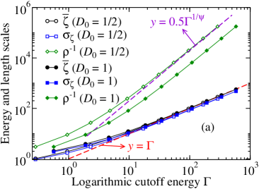
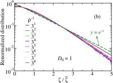
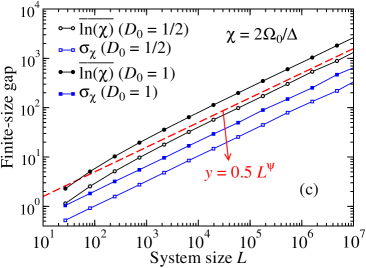
Figure 5: (a) The mean value of $\overline{\zeta}$, the standard deviation $\sigma_{\zeta}$ and the density of active spins $\rho$ as a function of the logarithmic cutoff energy $\Gamma=\ln\Omega_{0}/\Omega$ ($\Omega=\text{max$\left\{\lambda_{i}\right\}$ }$). (b) Snapshots of the coupling constant distributions at different densities $\rho$ along the SDRG flow. (c) The typical value of the finite-size gap as a function of the system size $L.$ We have considered chains of up to $L=3^{15}$ spins, with bare disorder strengths $D_{0}=1/2$ and $1$. Here, $\psi=\frac{1}{2}$. The error bars are about the size of the symbol sizes.

We first study the moments of the distribution of the renormalized couplings along the SDRG flow. As usual in the SDRG approach, it is convenient to define the logarithmic couplings $\zeta_{i}=\ln\left(\Omega/\lambda_{i}\right)$ and the logarithmic energy cutoff $\Gamma=\ln\left(\Omega_{0}/\Omega\right)$. We then study the mean value $\overline{\zeta}$ and standard deviation $\sigma_{\zeta}=\sqrt{\overline{\zeta^{2}}-\overline{\zeta}^{2}}$ as a function of $\Gamma$. Our results for $D_{0}=1/2$ and $D_{0}=1$ and system size of $L=3^{15}$ spins is shown in Fig. 5(a). Clearly, $\overline{\zeta}\approx\sigma_{\zeta}\approx\Gamma+\text{const}$ in the $\Gamma\rightarrow\infty$ limit. This implies an infinite-disorder fixed-point critical distribution. Thus, the SDRG method here employed is justified.

Next, we study the infinite-disorder fixed-point distribution. For comparison, that distribution for $p=1$ is well known (Fisher, 1994; Iglói, 2002; Hoyos et al., 2007b). It is

$$P_{p=1}^{*}\left(\lambda;\Omega\right)=\frac{1}{D_{\Gamma}\Omega}\left(\frac{\Omega}{\lambda}\right)^{1-1/D_{\Gamma}},$$ (40)

with $D_{\Gamma}=\Gamma+D_{0}$ [equivalent to $\pi^{*}\left(\zeta;\Gamma\right)=e^{-\zeta/D_{\Gamma}}/D_{\Gamma}$]. In Fig. 5(b), we show the distribution of log couplings at different stages of the SDRG flow for the case $D_{0}=1$. (We find statistically identical result for $D_{0}=1/2$ which is not shown for clarity.) After the initial stages of the SDRG flow, the fixed point is reached. Here, the different stages of the SDRG flow is parametrized by the density $\rho=N_{\Omega}/L$, where $N_{\Omega}$ is the number of active spins at the cutoff energy scale $\Omega$. Recall that, after each decimation step of the block SDRG procedure, $3$ spins are removed. Clearly, the fixed point distribution differs from the $p=1$ case Eq. (40) (dashed line $y=e^{-x}$), but only slightly. We attribute this small difference to the correlations arising among renormalized couplings under the flow.

The relation between energy and length scales along the SDRG flow is shown in Fig. 5(a). Simply the length scale $\rho^{-1}\sim\Gamma^{1/\psi}$ with universal tunneling exponent $\psi=1/2$. We also expect the finite-size gap $\Delta$ to obey the activated dynamical scaling (37). This is confirmed in our numerics as shown in Fig. 5(c). Both the mean value and the width of the distribution of $\ln\left(\Delta\right)$ behave similarly $\sim L^{\psi}$. Here, the finite-size gap is obtained by decimating the entire chain. The last decimated coupling constant $\tilde{\lambda}_{\text{final}}$ provides the finite-size gap $\Delta=2\tilde{\lambda}_{\text{final}}$.

IV.2.7 Thermodynamics and correlations

As the fixed-point distribution is of infinite-randomness type, the critical thermal entropy and specific heat behave similarly as in the $p=1$ case discussed in Sec. IV.1.3. The only difference is the residual entropy which modifies Eq. (21) to

$$S=\frac{2}{3}\left(1+\left(\frac{\sigma_{\ln\lambda}^{2}}{\ln\left(\frac{\Omega_{0}}{T}\right)}\right)^{1/\psi}\right)\ln 2,$$ (41)

the reasoning being that the ground state have degeneracy $2^{2L/3}$. The specific heat follows straightforwardly and recovers (22).

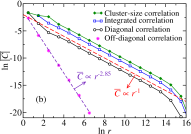
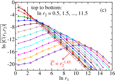
Figure 6: Average value of the spin correlations (42). (a) The average value of the spin correlation $\overline{\left|C(r_{1},r_{2})\right|}$ [see Eq. (42)] as a function of the internal spin-spin separations $r_{1}$ and $r_{2}$. (b) The average values of the diagonal $\overline{\left|C(r,r)\right|}$ (open circles), the off-diagonal $\overline{\left|C(r,2r)\right|}$ (stars), the integrated $\sum_{r_{2}}\overline{\left|C(r,r_{2})\right|}=\sum_{r_{1}}\overline{\left|C(r_{1},r)\right|}$ (open squares), and the cluster-size $\sum_{r_{1},r_{2}}\delta_{r,r_{1}+r_{2}}\overline{\left|C\left(r_{1},r_{2}\right)\right|}$ (closed diamonds) correlations. (c) The average correlation $\overline{\left|C(r_{1},r_{2})\right|}$ as a function of $r_{1}$ for different values of $r_{2}$. The system size is $L=3^{15}$ averaged over $1\,500$ disorder realizations which is sufficient to yield error bars of the size of the symbols. Solid lines are simple guide to the eyes.

In the SDRG framework, the ground-state spin correlation $C_{i,j,k}=\left\langle\sigma_{i}^{x}\sigma_{j}^{z}\sigma_{k}^{z}\right\rangle$ is $\pm 1$ if the spins $i<j<k$ are decimated together, and weakly vanishing (we set to zero) otherwise. To obtain the average value of $C_{i,j,k}$, we then build a normalized histogram $\overline{\left|C(r_{1},r_{2})\right|}$ in log-scale. After each SDRG decimation (decimation of spins $i$, $j$, and $k$), we add a unity to the bin ($r_{1},r_{2}$) if $\ln\left(j-i\right)$ is between $\ln r_{1}-\frac{1}{2}$ and $\ln r_{1}+\frac{1}{2}$, and $\ln\left(k-j\right)$ is between $\ln r_{2}-\frac{1}{2}$ and $\ln r_{2}+\frac{1}{2}$. This procedure is repeated until the entire chain is decimated and averaged over many disorder realizations. The histogram $\overline{\left|C(r_{1},r_{2})\right|}$ is then a proxy to average value of $C_{i,j,k}$, i.e.,

$$\overline{\left|C(r_{1},r_{2})\right|}=\overline{\left|\left\langle\sigma_{i}^{x}\sigma_{i+r_{1}}^{z}\sigma_{i+r_{1}+r_{2}}^{z}\right\rangle\right|}.$$ (42)

We plot in Fig. 6(a) the mean value of the spin correlation $\overline{C\left(r_{1},r_{2}\right)}$ as a function of the internal distances $r_{1}$ and $r_{2}$. Clearly, the correlation is maximum when $r_{1}=r_{2}$, as expected from symmetry.

In Fig. 6(b), we plot the diagonal correlation $\overline{C\left(r,r\right)}$, one of the possible off-diagonal correlations $\overline{C\left(r,2r\right)}$, the integrated correlation $\sum_{r_{2}}\overline{C\left(r,r_{2}\right)}=\sum_{r_{1}}\overline{C\left(r_{1},r\right)}$, and the cluster-size correlation $\sum_{r_{1}}\overline{\left|C\left(r_{1},r-r_{1}\right)\right|}=\sum_{r_{1},r_{2}}\delta_{r,r_{1}+r_{2}}\overline{\left|C\left(r_{1},r_{2}\right)\right|}$. They all vanish algebraically $\sim r^{-\phi}$, with universal exponent $\phi\approx 1$ but the off-diagonal correlations which vanishes as $\overline{C\left(r,2r\right)}\sim r^{-\varphi}$ with $\varphi\approx 1.85$.

In Fig. 6(c), we plot the average correlation $\overline{C\left(r_{1},r_{2}\right)}$ for various values of $r_{2}$. Interestingly, our numerical data indicates that $\overline{C\left(r_{1},r_{2}\right)}\sim r_{1}^{-\left(\varphi-\phi\right)}$ for fixed $r_{2}$ and $r_{1}\gg r_{2}$.

Analyzing these exponents for other sample sizes, we estimate their error to be of order $10\%$. Unfortunately, we do not have an analytical derivation for these exponents.

How about the typical value of these correlations? Typically, the triad of spins in (42) are not decimated together and, thus, develop quite weak correlations. As argued by Fisher (Fisher, 1994) and shown in many numerical works (Henelius and Girvin, 1998; Getelina and Hoyos, 2020; Wada and Hoyos, 2022) for the case $p=1$, this weak correlations are of order of the typical value of the coupling constants involved, $C_{\text{typ}}(r)\sim J_{\text{typ}}(r)$. Very plausible, this is also the case for any $p$ with the caveat that more than one coupling constant is involved. Thus, $C_{\text{typ}}\sim J_{\text{typ}}(r_{1})J_{\text{typ}}(r_{2})\dots J_{\text{typ}}(r_{p})$. Thus, from the dynamical scaling (10) we then conclude that the typical value of the correlations decays stretched exponentially fast with the spin separations. Roughly, we expect

$$C_{\text{typ}}\left(r_{1},r_{2}\right)\sim e^{-A\left(\ell\left(r_{1},r_{2}\right)\gamma_{D}\right)^{\psi}},$$ (43)

where $\ell(r_{1},r_{2})$ is a function which equals $\max\left\{r_{1},r_{2}\right\}$ for $r_{1}\gg r_{2}$ or $r_{2}\gg r_{1}$ and $\approx cr$ when $r_{1}\approx r_{2}\approx r$ (with $c$ being disorder-independent constant of order unity), $\gamma_{D}$ is a disorder-dependent Lyapunov exponent (Getelina and Hoyos, 2020; Wada and Hoyos, 2022) related to the clean-dirty crossover length (Laflorencie et al., 2004), and $A$ is a constant of order unity.

IV.2.8 Generalization to $p>2$

The usual SDRG method of Subsec. IV.2.1 can be easily generalized to any $p$. The key point is that new effective operators $\tilde{h}$ generated under the SDRG flow either commute or anticommutate and are of two-level type $\tilde{h}^{2}=\mathds{1}$. In this case, the only type of decimation that can take place is of second order in perturbation theory, and, thus, the renormalized coupling constants have the multiplicative structure of Eq. (28). As a consequence, the relation between length and timescales at a phase transition can only be of activated type Eq. (10), meaning that, at sufficiently strong disorder where the SDRG is applicable, the phase transition is governed by a infinite-randomness fixed point.

The analysis of the block SDRG flow of Subsec. IV.2.1 allowed us to conclude that this infinite-randomness critical point has tunneling exponent $\psi=\frac{1}{2}$ and very different mean and typical values of the correlation function for the cases $p=1$ and $2$. Although the generalization of the block SDRG method to other values of $p$ is not straightforward (as it involves many nontrivial projections, see Appendix A), it is plausible to conjecture that the phase transitions for uncorrelated disorder are governed by an analogous infinite-randomness critical point for any $p$. The tunneling exponent is universal and equals $\psi=\frac{1}{2}$. It not only governs the dynamical scaling but also the typical correlations. On the other hand, the exponent for the mean correlation function is universal, i.e., disorder independent, but does depend on the value of $p$.

A detailed and quantitative investigation of the critical behavior and of the associated Griffiths phases is out of the scope of the present work and is left for future research.

V Finite-size gap statistics

In this section, we present our numerically exact results on the spectral gap of the model Hamiltonian (1) for $p=2$. This quantity is computed from the roots of the polynomial as described in Sec. II and compared with the SDRG predictions described in Sec. IV.2.

V.1 Technical details

We refer the reader to Ref. Alcaraz et al., 2021 for useful numerical methods for calculating the roots of the polynomial (5)—(6). We emphasize that our method allow us to evaluate the finite-size gap in lattice sizes up to $\sim 10^{7}$ sites in the neighborhood of the transition lines with a numerical cost that grows linearly with the system size competing with the SDRG numerical cost. For systems that large, typically, the polynomials (5) have coefficients spanning in 500 orders of magnitude. Therefore, the entire evaluation of these coefficients can only be achieved using high numerical precision (500 digits). However, as shown in Ref. Alcaraz et al., 2021, we only need the last $100$ coefficients of the polynomial to obtain the finite-size gap with quadruple standard numerical precision (32 digits). When applying this method to our Hamiltonian, we found useful to keep the last coefficient of (5) always of order unity. This is accomplished by factorizing these coefficients when iterating the recursion relation (6). With that, the entire procedure can be accomplished using only standard routines in FORTRAN with quadruple precision.

V.2 Off-critical finite-size gap I

We start analyzing the off-critical Griffiths phases sketched in the phase diagram of Fig. 2(b). For such, we study three sets of chains: (set I) $\lambda_{A}$ is uniformly distributed in the interval $\left[0,0.2\right]$; (set II) $\lambda_{A}$ is uniformly distributed in the interval $\left[0.2,1.2\right]$; (set III) $\lambda_{A}$ is uniformly distributed in the interval $\left[0.5,1.5\right]$. In all cases, $\lambda_{B}$ is distributed uniformly in the interval $\left[0.5,1.5\right]$, and $\lambda_{C}$ is a constant (running from $1.2$ down to $0.9$) which serves as a tuning parameter. The running $\lambda_{C}$ passes through the critical point $\lambda^{*}=\lambda_{B,\text{typ}}=e^{\frac{3\ln 3-2\ln 2}{2}-1}\approx 0.95578$ [see Eq. (36)] but does not include it since the analysis of the critical system is reported in other sections. Notice that set III of chains is critical for $\lambda_{C}<\lambda_{C}^{*}$. For that reason, we consider only $\lambda_{C}>\lambda_{C}^{*}$ in this section.

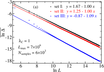
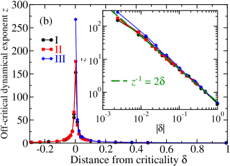
Figure 7: Finite-size gap analysis of the Griffiths phases in Fig. 2(b). The coupling constants $\left\{\lambda_{A,i}\right\}$ are uniformly distributed in the interval $\left[0,0.2\right]$ (set I), $\left[0.2,1.2\right]$ (set II) and $\left[0.5,1.5\right]$ (set III). In all cases, $\left\{\lambda_{B,i}\right\}$ are uniformly distributed in the interval $\left[0.5,1.5\right]$, and $\lambda_{C}$ is uniform and plays the role of a running parameter throughout the Griffiths phases. (a) The typical finite-size gap $\overline{\ln\Delta}$ as a function of the system size $L$ for $\lambda_{C}=1$. The data is averaged over $N_{\text{samples}}=6\,000$ disorder realizations and the error bars are about the size of the data points. Linear fits for the data are provided in the legends from which the dynamical exponent $z$ is obtained. The best fits are restricted to system sizes $L>10^{6}$. (b) The dynamical exponent $z$ as a function of the distance from criticality Eq. (36). Lines are guide to the eyes. Inset: same data in the main panel in log-log scale. The dashed line is the SDRG asymptotic behavior ($\delta\ll 1$) $z=1/(2\delta)$.

In case I, we explore the interplay between the two strongest couplings $\lambda_{B}$ and $\lambda_{C}$ while $\lambda_{A}$ is a much weaker coupling. The Rare Regions are of $B$-type inside a bulk in the $C$ phase. In case II, the value of $\lambda_{A}$ is increased such that some Rare Regions of $A$-type also appear. Finally, in case III, both Rare Regions of $A$- and $B$-type appear equally. At the final point $\lambda_{C}=\lambda_{C}^{*}$, the multicritical point is reached.

In Fig. 7(a) we show the relation between $\overline{\ln\Delta}$ (with $\Delta$ being the system finite-size gap) and the system size $L$ for $\lambda_{C}=1$. From this, we can obtain the off-critical dynamical exponent $z$ by fitting $\Delta\sim L^{-z}$ to the data. Repeating this procedure for other values of $\lambda_{C}$, we determine how $z$ diverges as the critical point is approached, see Fig. 7(b). It diverges as $z\approx 1/\left(2\delta\right)$, with $\delta$ being the distance from criticality as defined in (36). We emphasize that this numerically exact result is in agreement with the SDRG analytical predictions in the $z\rightarrow\infty$ limit.

V.3 Off-critical finite-size gap II

We now study the case in which only one of the couplings is disordered, say, $\lambda_{A}$ uniformly distributed in the interval $\left[0,0.2\right]$. The corresponding phase diagram is shown in Fig. 2(a). Here, we focus on the off-critical region near the transition between the $B$- and $C$-phases. Notice that there are no Griffiths phases surrounding the transition for sufficiently small $\lambda_{A,\text{typ}}$. Thus, the gap is vanishing only at the transition point $\lambda_{B}=\lambda_{C}$. Closer to the multicritical point, Griffiths phases appear.

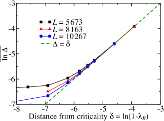
Figure 8: The typical value of the system gap $\Delta$ as a function of the distance from criticality $\delta=\ln\left(1-\lambda_{B}\right)$ for chains of different sizes $L$. The coupling constants are such that $\lambda_{A}$ is uniformly distributed in the interval $\left[0,0.2\right]$, and $\lambda_{B}$ and $\lambda_{C}$ are homogeneous with $\lambda_{C}=1$ and $\lambda_{B}$ being the tuning parameter. The data is average over $N_{\text{samples}}=1\,500$ disorder realizations. The error bars are about the symbol sizes. Solid lines are simple guide to the eyes. The dashed line is the clean behavior in the thermodynamic limit: $\Delta\sim\delta^{\phi_{\Delta}}$, with $\phi_{\Delta}=1$.

We plot in Fig. 8 the typical value of the system gap $\Delta$ as a function of the distance from criticality $\delta$. Since $\lambda_{C}$ and $\lambda_{B}$ are homogeneous, the definition (18) is not useful because of the vanishing denominator. Here, we simply use $\delta=\ln\left(\lambda_{C}-\lambda_{B}\right)$. Also, we fix $\lambda_{C}=1>\max\left\{\lambda_{A}\right\}$ and use $\lambda_{B}$ as a running parameter. Notice that $\Delta$ diminishes as in the clean system: $\Delta\sim\delta$. For small $\delta$, $\Delta$ saturates due to finite-size effects, meaning that the correlation length is greater than $L$. We recall that our method is not optimal for gapful systems. This is because larger the gap larger is the number of coefficients required in the characteristic polynomial (Alcaraz et al., 2021). For that reason, we studied chains of “small” sizes up to $10\,267$ sites.

Having shown the absence of Griffiths phases far from the multicritical point ($\lambda_{C}>\max\left\{\lambda_{A}\right\}$), we now show their existence otherwise. We thus study chains in which $\lambda_{C}=1$, $\lambda_{A}$ is uniformly distributed in the interval $\left[0,e\lambda_{A,\text{typ}}\right]$, and $\lambda_{B}$ is the tuning parameter. We report that the finite-size gap vanishes as $\Delta\sim L^{-z}$ [as in Fig. 7(a)], with the value of the off-critical dynamical exponent $z$ increasing up to a finite value as the transition is approached, see Fig. 9. Notice that far from the critical point $\lambda_{B}=1$, the off-critical dynamical exponent is practically insensitive to the distance from criticality $\delta=1-\lambda_{B}$ as the low-energy behavior is dominated by Rare Regions which are locally in the $A$ phase.

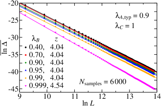
Figure 9: The typical value of the finite-size gap $\Delta$ as a function of the system size $L$. The couplings $\lambda_{B}$ and $\lambda_{C}$ are nonrandom and their values are given in the legends. The coupling $\lambda_{A}$ is a independent random variable uniformly distributed in the interval $\left[0,0.9e\right]$ (thus, typical value $\lambda_{A,\text{typ}}=0.9$). The data is average over $N_{\text{samples}}=6\,000$ disorder realizations. The error bars are about the symbol sizes. Solid lines are best fits to Eq. (9) in the region $L>e^{12}$. The corresponding Griffiths dynamical exponent are given in the legends.

V.4 Critical finite-size gap statistics I

We now address the infinite-randomness critical lines, the dashed lines in the phase diagram of Fig. 2(a) and (b). To illustrate universality, we consider two cases: (chain A) $\lambda_{A}$ and $\lambda_{B}$ are, respectively, uniformly distributed in the intervals $\left[0,0.2\right]$ and $\left[0.5,1.5\right]$, and $\lambda_{C}$ is homogeneous and equals $\lambda_{B,\text{typ}}=e^{\frac{3\ln 3-2\ln 2}{2}-1}\approx 0.95578$ (ensuring criticality); and (chain B) $\lambda_{A}$, $\lambda_{B}$, and $\lambda_{C}$ are, respectively, uniformly distributed in the intervals $\left[0,0.5\right]$, $\left[0,1\right]$, and $\left[0,1\right]$.

In Fig. 10 we plot the typical value of the finite-size gap [and the corresponding Laguerre bound $\Delta_{\text{LB}}$, see Eqs. (7)—(10)] for those critical chains as a function of the system size $L$. As expected from the activated dynamical scaling (10), the finite-size gap vanishes stretched exponentially fast with universal (i.e., disorder-independent) tunneling exponent $\psi=1/2$, compatible with the asymptotic behavior ($L\gg 1$) of our data. We call attention to the fact that $\Delta$ and $\Delta_{\text{LB}}$ become virtual indistinguishable for $L\gg 1$. This feature was already noticed for the case $p=1$ (Alcaraz et al., 2021). We conjecture that finite-size values of $\Delta_{\text{LB}}\rightarrow\Delta$ for $L\rightarrow\infty$ in the case of infinite-randomness criticality. As argued in Ref. Alcaraz et al., 2021, this is because the largest root of the characteristic polynomial separates from the other ones as $L$ increases. Thus, only the few largest coefficients of the polynomial are necessary to accurately compute it (see Sec. V.1).

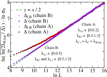
Figure 10: Finite-size gap $\Delta$ (and the corresponding Laguerre bound $\Delta_{\text{LB}}$) as a function of the system size for chains A and B (see text). The typical value is compatible with activated dynamical scaling $\overline{\ln\Delta}\sim-L^{\psi}$, with universal (disorder-independent) tunneling expoente $\psi=\frac{1}{2}$, see dashed line and Eq. (37). The data is averaged over $N_{\text{samples}}=10^{3}$ ($4\times 10^{4}$) disorder realizations for chain A (B), and the error bars are about the symbol sizes.

V.5 Critical finite-size gap statistics II

Here, we investigate the intriguing critical line in which the two major couplings are uniform, i.e., the horizontal boundary line in the phase diagram Fig. 2(a). Thus, we take $\lambda_{B}=\lambda_{C}=1$ and $\lambda_{A}$ uniformly distributed between $0$ and $e\lambda_{A,\text{typ}}$. The typical value of the $A$ couplings, $\lambda_{A,\text{typ}}$, is used as a tuning parameter and reaches the multicritical point when $\lambda_{A,\text{typ}}=1$.

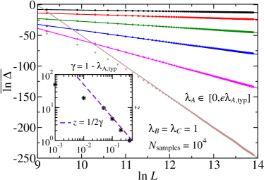
Figure 11: The typical value of the finite-size gap $\Delta$ as a function of the system size $L$ for chains with homogeneous coupling constants $\lambda_{B}=\lambda_{C}=1$ and $\left\{\lambda_{A}\right\}$ uniformly distributed in the interval $\left[0,e\times\lambda_{A,\text{typ}}\right]$ for various values of the tuning parameter (from top to bottom) $\lambda_{A,\text{typ}}=0.6$, $0.8$, $0.9$, $0.95$, $0.99$, and $0.999$. The data is averaged over $N_{\text{samples}}=10^{4}$ disorder realizations and the error bars are about the symbol sizes. The solid lines are best linear fits to $\overline{\ln\Delta}\sim-z\ln L$ (constrained to $L>e^{13}$) from which the critical dynamical exponent is obtained (respectively, $z=1.00$, $2.08$, $4.56$, $9.76$, $19.48$, and $49.82$) and shown in the inset as a function of the distance from the multicritical point $\gamma=1-\lambda_{A,\text{typ}}$.

Our results are shown in Fig. (11). Clearly, sufficiently far from the multicritical point ($\lambda_{A,\text{typ}}\leq\lambda_{A,\text{typ}}^{*}\sim 0.6$) the critical point is in the clean Ising universality class $z=1$ [solid line in Fig. 2(a)]. Approaching the multicritical point ($\lambda_{A,\text{typ}}>\lambda_{A,\text{typ}}^{*}$), a line of finite-disorder fixed points [dotted line in Fig. 2(a)] is tuned with varying critical dynamical exponent $z$ that diverges as the multicritical point is approached (see inset). For comparison, we show the line $z=\left(2\gamma\right)^{-1}$ as predicted by the SDRG method when $\gamma=1-\lambda_{A,\text{typ}}\rightarrow 0$. This seems to be the trend for $\gamma\apprge 0.01$. We cannot rule out that we are plagued by finite-size effect for smaller $\gamma$.

V.6 multicritical finite-size gap statistics

Here, we finally investigate the multicritical point. We find that in both phase diagrams of Fig. 2, the multicritical point is of infinite-randomness type with universal tunneling exponent $\psi=1/2$.

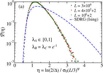
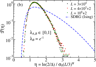
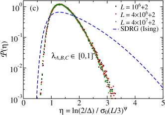
Figure 12: Finite-size gap distribution ${\cal P}$ for different system sizes $L$. The finite-size gap $\Delta$ is rescaled according to the scaling variable $\eta$ in Eq. (37). The coupling constants are either homogeneous equal to $e^{-1}$ or uniformly distributed in the interval $\left[0,1\right]$ as indicated in the legends. The width $\sigma_{0}$ is, respectively, $\sqrt{1/3}$, $\sqrt{2/3}$, and $1$ in panels (a), (b), and (c). The normalized histograms were built using $10^{5}$ to $10^{6}$ disorder realizations. The dashed line is the SDRG prediction (19) for the transverse-field Ising chain ($p=1$).

In Fig. 12 we plot the distribution ${\cal P}$ of the finite-size gap $\Delta$ properly rescaled according to Eq. (37) for various system lengths and disorder parameters. Clearly, the scaling variable $\eta$ is sufficient to produce that data collapse for the system sizes used and this gives us further confidence on the activated dynamical scaling (10) with universal (disorder-independent) tunneling exponent $\psi=1/2$. We notice, in addition, that the probability distribution ${\cal P}$ is not universal and is weakly dependent on the disorder details. Furthermore, ${\cal P}$ is quite different from the SDRG prediction Eq. (19) for the transverse-field Ising chain ($p=1$), even though they are governed by the same infinite-disorder fixed point. Finally, we report (not shown for clarity) that this distribution depends on the modularity of the lattice size $L$, i.e., ${\cal P}\left(\eta\right)$ depends on $L\mod 3$. This is not a surprise since a similar difference also appears in the clean system. There, the finite-size gap amplitudes also depend on the modularity, i.e., $\Delta\sim aL^{-z}$ with $a\equiv a\left(L\mod 3\right)$.

VI Conclusions

We have studied the effects of quenched disorder on a family of free fermionic models (1) with $(p+1)$-multispin interaction, paying special attention to the case $p=2$ corresponding to the random version of the three-spin interacting Fendley model.

When all the coupling constants are generically disordered, the clean phase transitions (including the multicritical points) are destabilized. The replacing transition is of infinite-randomness character where the critical dynamical scaling is activated (10) with universal (disorder- and $p$-independent) tunneling exponent $\psi=1/2$. This exponent governs the low-temperature singular thermodynamic behavior. The average value of the correlation functions are also universal and decay algebraically with the spin separations. We do not have an analytical theory for those exponents and a detailed study is left for future research. The typical value of the correlations, on the other hand, behaves quite differently. It decays stretched exponentially fast with the spin-spin separation. In addition, strong Griffiths singularities surround the transitions. Although the system is noncritical with short-range correlations, the spectral gap vanishes. The singularities are related to the slow dynamics of the domain walls surrounding the so-called rare regions. This phenomena is very similar to the domain-wall-induced (or rare-regions-induced) Griffiths singularities in the dimerized XXZ spin-1/2 chain and in the random transverse-field Ising model.

When only one (of few) type of coupling constants are disordered, the scenario is more involved. When the disordered coupling is weak, the singular critical behavior of the clean system is stable and there is no surrounding Griffiths phases. Upon increasing the magnitude of the disordered coupling, the universality of the transition changes and is of finite-randomness character. The critical scaling is power-law conventional (9) but with nonuniversal (disorder-dependent) dynamical critical exponent $z$. The increasing of the magnitude of the disordered couplings yields to another effect. It nucleates rare regions which contributes to off-critical Griffiths singularities. Interestingly, the finite-randomness criticality extends up to the multicritical point.

Although we have explicitly worked out those results for the cases of $p=1$ and $2$, from symmetry grounds we expect them to be valid for all $p$ in the family model (1) for sufficiently large disorder. Evidently, we cannot exclude other scenarios appearing when $p$ is very large and disorder is weak.

Finally, the agreement between our numerically exact results obtained for quite large lattice sizes (up to $L\sim 10^{7}$ sites) with the “block” SDRG is remarkable. We stress that the SDRG methed is not an exact one. It took more than a decade after its conception to realize that it can provide asymptotically exact critical exponents and other universal quantities. This was accomplished comparing the SDRG with exact diagonalization of a few models such as the transverse-field Ising chain and the XX spin-1/2 chain and for moderate lattice sizes ($L\sim 10^{3}$) and the Heisenberg chain ($L\sim 200$). Here, we have the rare opportunity to show that this is also true for a different family of models and for quite large chains.

We believe that our method for evaluating the finite-size gaps for large system sizes with minimal numerical cost ($\sim L$) will be a useful tool to study the effects of disorder in the phase transition of other systems.

Appendix A The block SDRG method

Here, we derive another SDRG decimation procedure. We follow the idea of Ref. Hoyos, 2008 where a larger block spin is considered. It was initially devised to enable the SDRG approach to tackle cases where the bare disorder in the system is weak. It was important to correct the SDRG flow from nonphysical features introduced by the simpler perturbative approach (as in Sec. IV). Here, this approach has a fundamentally different appeal. It consider the largest spin block in which there are only two energy levels. The projection is, thus, onto a richer ground-state which may capture additional features neglected in the simplest approach.

A.1 Case $p=1$

Let us start with the simpler case where $p=1$. For convenience we rewrite the Hamiltonian as

$$H=\sum_{i}\left\{-\lambda_{A,i}h_{A,i}-\lambda_{B,i}h_{B,i}\right\},$$ (44)

where $h_{A,i}=\sigma_{2i-1}^{x}\sigma_{2i}^{z}$ and $h_{B,i}=\sigma_{2i}^{x}\sigma_{2i+1}^{z}$.

Following the SDRG philosophy, we search for the local Hamiltonian which exhibits the largest energy gap between its two energy levels. As the largest spin block still exhibiting only two energy levels is either $-\lambda_{A,i}h_{A,i}-\lambda_{B,i}h_{B,i}$ or $-\lambda_{B,i}h_{B,i}-\lambda_{A,i+1}h_{A,i+1}$, we then define the energy cutoff as $\Omega=\max\left\{\sqrt{\lambda_{A,i}^{2}+\lambda_{B,i}^{2}}\right\}$.

Say that $\Omega=\sqrt{\lambda_{A,2}^{2}+\lambda_{B,2}^{2}}$. In this case, we treat $H_{0}=-\lambda_{A,2}h_{A,2}-\lambda_{B,2}h_{B,2}$ exactly and project the operators $H_{1}=-\lambda_{B,1}h_{B,1}-\lambda_{A,3}h_{A,3}$ onto its ground-state subspace. More precisely, we are interested in the projections of the operators $\sigma_{3}^{z}$ and $\sigma_{5}^{x}$. The ground-state subspace of $H_{0}$ is spanned by $\left|s_{3},s_{5}\right\rangle=\left|s_{3}\right\rangle\otimes\left(\cos\theta\left|\uparrow_{4}\right\rangle+\sin\theta\left|\downarrow_{4}\right\rangle\right)\otimes\left|s_{5}\right\rangle$, where $\sigma_{3}^{x}\left|s_{3}\right\rangle=s_{3}\left|s_{3}\right\rangle$, $\sigma_{5}^{z}\left|s_{5}\right\rangle=s_{5}\left|s_{5}\right\rangle$, $\cos\theta=\lambda_{B,2}s_{5}/\sqrt{2\Omega\left(\Omega-\lambda_{A,2}s_{3}\right)}$, and $\sin\theta=\left(\Omega-\lambda_{A,2}s_{3}\right)/\sqrt{2\Omega\left(\Omega-\lambda_{A,2}s_{3}\right)}$. The projected operators are, thus, $\tilde{\sigma}_{3}^{z}=\left|\lambda_{B,2}\right|\tilde{\sigma}^{z}/\Omega$ and $\tilde{\sigma}_{5}^{x}=-\lambda_{A,2}\tilde{\sigma}^{x}\tilde{\tau}^{x}/\Omega$, where the effective spin-1/2 degrees of freedom $\tilde{\boldsymbol{\sigma}}$ and $\tilde{\boldsymbol{\tau}}$ span the ground-state subspace with $\tilde{\sigma}^{x}\left|s_{3},s_{5}\right\rangle=s_{3}\left|s_{3},s_{5}\right\rangle$ and $\tilde{\tau}^{z}\left|s_{3},s_{5}\right\rangle=s_{5}\left|s_{3},s_{5}\right\rangle$. Therefore, the renormalized Hamiltonian is

$$\tilde{H}_{1}=-\tilde{\lambda}_{B,1}\tilde{h}_{B,1}-\tilde{\lambda}_{A,3}\tilde{h}_{A,3},$$ (45)

where $\tilde{h}_{B,1}=\sigma_{2}^{x}\tilde{\sigma}^{z}$, $\tilde{h}_{A,3}=\tilde{\sigma}^{x}\tilde{\tau}^{x}\sigma_{6}^{z}$, $\tilde{\lambda}_{B,1}=\lambda_{B,1}\left|\lambda_{B,2}\right|/\Omega$, and $\tilde{\lambda}_{A,3}=-\lambda_{A,2}\lambda_{A,3}/\Omega$. Notice that the algebra (3) is preserved in the renormalized system. In addition, the extra degree of freedom $\tilde{\boldsymbol{\tau}}$ appears only in $\tilde{h}_{A,3}$, and, thus, we interpret the renormalized chain as being two new chains where the renormalized operators are $\tilde{h}_{B,1}=\sigma_{2}^{x}\tilde{\sigma}^{z}$, $\tilde{h}_{A,3}=\tilde{\sigma}^{x}\sigma_{6}^{z}$ in both chains. The corresponding renormalized couplings are $\tilde{\lambda}_{B,1}=\lambda_{B,1}\left|\lambda_{B,2}\right|/\Omega$ and $\tilde{\lambda}_{A,3}=\mp\lambda_{A,2}\lambda_{A,3}/\Omega$.

In the regime of interest where $\lambda_{A,2}$ and $\lambda_{B,2}$ are very distinct from each other, say, $\lambda_{B,2}\gg\lambda_{A,2}$, then $\Omega\rightarrow\left|\lambda_{B,2}\right|$, the renormalized operator $\tilde{\boldsymbol{\sigma}}\rightarrow\boldsymbol{\sigma}_{3}$, and the renormalized couplings become $\tilde{\lambda}_{B,1}=\lambda_{B,1}$ and $\tilde{\lambda}_{A,3}=\mp\lambda_{A,2}\lambda_{A,3}/\left|\lambda_{B,2}\right|$, which recovers the usual SDRG result (15). If, on the other hand, $\lambda_{B,2}\ll\lambda_{A,2}$, then $\Omega\rightarrow\left|\lambda_{A,2}\right|$ and the renormalized couplings become $\tilde{\lambda}_{B,1}=\lambda_{B,1}\left|\lambda_{B,2}\right|/\left|\lambda_{A,2}\right|$ and $\tilde{\lambda}_{A,3}=\mp\lambda_{A,3}$, which, at first glance, does not seem to recover the usual SDRG result (15). This is not the case. One can correct the signs of the couplings by appropriately redefining the effective spin-1/2 degrees of freedom $\tilde{\boldsymbol{\sigma}}$ and $\tilde{\boldsymbol{\tau}}$.

In sum, the block SDRG approach here derived is similar to the usual SDRG derived in Sec. IV.1. Qualitatively, they are the same in the sense that 2 original operators are removed from the system in each decimation step and that the renormalized couplings are smaller than the original ones (both approaches are self-consistent). The only difference is quantitative: the effective couplings are renormalized differently. However, this difference vanishes in the strong-disorder limit.

A.2 Case $p=2$

The Hamiltonian of interest is

$$H=\sum_{i}\left\{-\lambda_{A,i}h_{A,i}-\lambda_{B,i}h_{B,i}-\lambda_{C,i}h_{C,i}\right\},$$ (46)

where $h_{A,i}=\sigma_{3i-2}^{x}\sigma_{3i-1}^{z}\sigma_{3i}^{z}$, $h_{B,i}=\sigma_{3i-1}^{x}\sigma_{3i}^{z}\sigma_{3i+1}^{z}$, and $h_{C,i}=\sigma_{3i}^{x}\sigma_{3i+1}^{z}\sigma_{3i+2}^{z}$.

Following the block SDRG philosophy, we search for the largest local coupling $\Omega=\max\left\{\left|\lambda_{A,i}\right|,\left|\lambda_{B,i}\right|,\left|\lambda_{C,i}\right|\right\}$, say, $\Omega=\left|\lambda_{B,2}\right|$, and consider the largest block of operators which still exhibits only two energy levels. Thus, we consider as unperturbed Hamiltonian $H_{0}=-\lambda_{A,2}h_{A,2}-\lambda_{B,2}h_{B,2}-\lambda_{C,2}h_{C,2}$. The renormalized system is obtained by projecting $h_{B,1}$, $h_{C,1}$, $h_{A,3}$, and $h_{B,3}$ onto the ground-state subspace of $H_{0}$.

The construction of the eigenstates of $H_{0}$ is straightforward but tedious. There are only two energy levels with energies $\pm E$, where $E=\sqrt{\lambda_{A,2}^{2}+\lambda_{B,2}^{2}+\lambda_{C,2}^{2}}$. Each level is $2^{4}$ degenerate as $H_{0}$ involves $5$ spins-1/2 (spins $\boldsymbol{\sigma}_{4,5,\dots,8}$). The ground-state manifold is the set $\left\{\left|g_{s_{4},s,s_{7},s_{8}}\right\rangle\right\}$ where $\left|g_{s_{4},s,s_{7},s_{8}}\right\rangle=\left|s_{4},s_{7},s_{8}\right\rangle\otimes\left|s_{s_{4},s_{7},s_{8}}\right\rangle$ since $H_{0}$ is diagonal in the operators $\sigma_{4}^{x}$, $\sigma_{7}^{z}$, and $\sigma_{8}^{z}$. Here, $\sigma_{4}^{x}\left|g_{s_{4},s,s_{7},s_{8}}\right\rangle=s_{4}\left|g_{s_{4},s,s_{7},s_{8}}\right\rangle$, $\sigma_{7}^{z}\left|g_{s_{4},s,s_{7},s_{8}}\right\rangle=s_{7}\left|g_{s_{4},s,s_{7},s_{8}}\right\rangle$, $\sigma_{8}^{z}\left|g_{s_{4},s,s_{7},s_{8}}\right\rangle=s_{8}\left|g_{s_{4},s,s_{7},s_{8}}\right\rangle$, and the two states $\left|s_{s_{4},s_{7},s_{8}}\right\rangle$ ($s=\pm 1$) encodes the states of spins $5$ and $6$. They are

$$\left|\pm_{s_{4},s_{7},s_{8}}\right\rangle=\frac{\left|a_{\vec{s}}\right\rangle+\left|b_{\vec{s}}\right\rangle}{2\sqrt{1+\left\langle b_{\vec{s}}|a_{\vec{s}}\right\rangle}}\pm\frac{\left|a_{\vec{s}}\right\rangle-\left|b_{\vec{s}}\right\rangle}{2\sqrt{1-\left\langle b_{\vec{s}}|a_{\vec{s}}\right\rangle}},$$

where

$$\left|a_{\vec{s}}\right\rangle = \left|a_{s_{4},s_{7},s_{8}}\right\rangle=N_{-}\left[\lambda_{C,2}s_{7}s_{8}\left|\rightarrow_{5},\uparrow_{6}\right\rangle\right.$$

$$\left.+\left(E-\lambda_{B,2}s_{7}\right)\left|\rightarrow_{5},\downarrow_{6}\right\rangle-\lambda_{A,2}s_{4}\left|\leftarrow_{5},\downarrow_{6}\right\rangle\right],$$

$$\left|b_{\vec{s}}\right\rangle = \left|b_{s_{4},s_{7},s_{8}}\right\rangle=N_{+}\left[\left(E+\lambda_{B,2}s_{5}\right)\left|\rightarrow_{5},\uparrow_{6}\right\rangle\right.$$

$$\left.+\lambda_{C,2}s_{7}s_{8}\left|\rightarrow_{5},\downarrow_{6}\right\rangle+\lambda_{A2}s_{4}\left|\leftarrow_{5},\uparrow_{6}\right\rangle\right],$$

$N_{\pm}=1/\sqrt{2E\left(E\pm\lambda_{B,2}s_{7}\right)}$ are normalization constants, and $\left\langle b_{\vec{s}}|a_{\vec{s}}\right\rangle=s_{7}s_{8}\lambda_{C,2}/\sqrt{\lambda_{A2}^{2}+\lambda_{C2}^{2}}$.

We define the four spin-1/2 operators $\tilde{\boldsymbol{\sigma}}_{4}$, $\tilde{\boldsymbol{\sigma}}$, $\tilde{\boldsymbol{\sigma}}_{7}$, and $\tilde{\boldsymbol{\sigma}}_{8}$ which span the ground-state subspace in the following manner: $\tilde{\sigma}_{4}^{x}\left|g_{s_{4},s,s_{7},s_{8}}\right\rangle=s_{4}\left|g_{s_{4},s,s_{7},s_{8}}\right\rangle$, $\tilde{\sigma}^{z}\left|g_{s_{4},s,s_{7},s_{8}}\right\rangle=s\left|g_{s_{4},s,s_{7},s_{8}}\right\rangle$, $\tilde{\sigma}_{7}^{z}\left|g_{s_{4},s,s_{7},s_{8}}\right\rangle=s_{7}\left|g_{s_{4},s,s_{7},s_{8}}\right\rangle$, and $\tilde{\sigma}_{8}^{z}\left|g_{s_{4},s,s_{7},s_{8}}\right\rangle=s_{8}\left|g_{s_{4},s,s_{7},s_{8}}\right\rangle$.

We are now ready to project the $H_{1}$ onto the ground states of $H_{0}$. Let us start by projecting the operator $\sigma_{4}^{z}$. The matrix element is

$$\left\langle g_{t_{4},t,t_{7},t_{8}}\left|\sigma_{4}^{z}\right|g_{s_{4},s,s_{7},s_{8}}\right\rangle =\delta_{s_{4},-t_{4}}\delta_{s_{7},t_{7}}\delta_{s_{8},t_{8}}\left\langle t_{-s_{4},s_{7},s_{8}}|s_{s_{4},s_{7},s_{8}}\right\rangle$$

$$=\frac{\delta_{s_{4},-t_{4}}\delta_{s_{7},t_{7}}\delta_{s_{8},t_{8}}}{\sqrt{\lambda_{A,2}^{2}+\lambda_{C,2}^{2}}} \left(-\frac{\left|\lambda_{A,2}\right|\lambda_{B,2}s_{7}s\delta_{s,t}}{E}+s_{7}s_{8}\lambda_{C,2}\delta_{s,-t}\right).$$

Thus, the projected operator is

$$\tilde{\sigma}_{4}^{z}\left(-\frac{\left|\lambda_{A,2}\right|\lambda_{B,2}}{E\sqrt{\lambda_{A,2}^{2}+\lambda_{C,2}^{2}}}\tilde{\sigma}^{z}\tilde{\sigma}_{7}^{z}+\frac{\lambda_{C,2}}{\sqrt{\lambda_{A,2}^{2}+\lambda_{C,2}^{2}}}\tilde{\sigma}^{x}\tilde{\sigma}_{7}^{z}\tilde{\sigma}_{8}^{z}\right).$$

Similarly, projecting $\sigma_{8}^{x}$, $\sigma_{7}^{x}\sigma_{8}^{z}$, and $\sigma_{4}^{z}\sigma_{5}^{z}$ we obtain, respectively,

$$\frac{\left|\lambda_{A,2}\right|}{\sqrt{\lambda_{A,2}^{2}+\lambda_{C,2}^{2}}}\tilde{\sigma}_{8}^{x}-\frac{\lambda_{B,2}\lambda_{C,2}}{E\sqrt{\lambda_{A,2}^{2}+\lambda_{C,2}^{2}}}\tilde{\sigma}^{y}\tilde{\sigma}_{8}^{y},$$

$$\frac{\left|\lambda_{A,2}\right|}{E}\tilde{\sigma}_{7}^{x}\tilde{\sigma}_{8}^{z},\mbox{ and }-\text{sign}\left(\lambda_{A,2}\right)\frac{\lambda_{C,2}}{E}\tilde{\sigma}_{4}^{y}\tilde{\sigma}^{y}\tilde{\sigma}_{7}^{z}\tilde{\sigma}_{8}^{z}.$$

Collecting all those terms, we find that $\tilde{H}_{1}=-\tilde{\lambda}_{B,1}\tilde{h}_{B,1}-\tilde{\lambda}_{C,1}\tilde{h}_{C,1}-\tilde{\lambda}_{A,3}\tilde{h}_{A,3}-\tilde{\lambda}_{B,3}\tilde{h}_{B,3},$ where

$$\tilde{\lambda}_{C,1}=-\text{sign}\left(\lambda_{A,2}\right)\frac{\lambda_{C,1}\lambda_{C,2}}{E},\ \tilde{h}_{C,1}=\sigma_{3}^{x}\tilde{\sigma}_{4}^{y}\tilde{\sigma}^{y}\tilde{\sigma}_{7}^{z}\tilde{\sigma}_{8}^{z},$$

$$\tilde{\lambda}_{A,3}=\frac{\left|\lambda_{A,2}\right|\lambda_{A,3}}{E},\ \tilde{h}_{A,3}=\tilde{\sigma}_{7}^{x}\tilde{\sigma}_{8}^{z}\sigma_{9}^{z},$$

$$\tilde{\lambda}_{B,1}\tilde{h}_{B,1}=\lambda_{B,1}\sigma_{2}^{x}\sigma_{3}^{z}\tilde{\sigma}_{4}^{z}\left(\frac{\lambda_{C,2}E\tilde{\sigma}^{x}\tilde{\sigma}_{8}^{z}-\left|\lambda_{A,2}\right|\lambda_{B,2}\tilde{\sigma}^{z}}{E\sqrt{\lambda_{A,2}^{2}+\lambda_{C,2}^{2}}}\right)\tilde{\sigma}_{7}^{z},$$

$$\tilde{\lambda}_{B,3}\tilde{h}_{B,3}=\lambda_{B,3}\left(\frac{\left|\lambda_{A,2}\right|E\tilde{\sigma}_{8}^{x}-\lambda_{B,2}\lambda_{C,2}\tilde{\sigma}^{y}\tilde{\sigma}_{8}^{y}}{E\sqrt{\lambda_{A,2}^{2}+\lambda_{C,2}^{2}}}\right)\sigma_{9}^{z}\sigma_{10}^{z}.$$

A.2.1 The algebra of the renormalized operators

As in the simpler SDRG approach (Sec. IV.2) the algebra (3) is not preserved. However, it is almost preserved. The only operators changing the algebra structure are the operators $\tilde{h}_{B,1}$ and $\tilde{h}_{B,3}$. They anticommutate with the nearest- and next-nearest-neighbor operators and commute with the farther-neighbor operators, preserving the algebra (3). However, they do not commute with each other. Instead, $\left[\tilde{\lambda}_{B,1}\tilde{h}_{B,1},\tilde{\lambda}_{B,3}\tilde{h}_{B,3}\right]\propto\lambda_{B,1}\lambda_{A,2}\lambda_{C,2}\lambda_{B,3}/E^{2}.$ Interestingly, in the regime $\left|\lambda_{B,2}\right|\gg\left|\lambda_{A,2}\right|,\left|\lambda_{C,2}\right|$ (which is the one we are interested in), they can be considered commuting operators since

$$\frac{\left[\tilde{\lambda}_{B,1}\tilde{h}_{B,1},\tilde{\lambda}_{B,3}\tilde{h}_{B,3}\right]}{E_{B,1}E_{B,3}}\mbox{ is of order }{\cal O}\left(\frac{\lambda_{A,2}\lambda_{C,2}}{\lambda_{B,2}^{2}}\right)\rightarrow 0,$$ (47)

where $\pm E_{B,1}$ ($\pm E_{B,3}$) are the energy levels of $\tilde{h}_{B,1}$ ($\tilde{h}_{B,3}$). Precisely,

$$E_{B,1}=\left|\lambda_{B,1}\right|\sqrt{\frac{\lambda_{C,2}^{2}}{\lambda_{A,2}^{2}+\lambda_{C,2}^{2}}+\frac{\lambda_{A,2}^{2}}{\lambda_{A,2}^{2}+\lambda_{C,2}^{2}}\left(\frac{\lambda_{B,2}}{E}\right)^{2}}.$$

(The value of $E_{B,3}$ is that of $E_{B,1}$ with $\lambda_{B,1}$ replaced by $\lambda_{B,3}$ and $\lambda_{A,2}$ interchanged with $\lambda_{C,2}$.) In the regime $\left|\lambda_{B,2}\right|\gg\left|\lambda_{A,2}\right|,\left|\lambda_{C,2}\right|$, then $E_{B,1}\approx\left|\lambda_{B,1}\right|$ and $E_{B,3}\approx\left|\lambda_{B,3}\right|$. In addition, the renormalized operators simplify to

$$\tilde{h}_{B,1}=\sigma_{2}^{x}\sigma_{3}^{z}\tilde{\sigma}_{4}^{z}\left(\frac{\lambda_{C,2}\tilde{\sigma}^{x}\tilde{\sigma}_{8}^{z}-\text{sign}\left(\lambda_{B,2}\right)\left|\lambda_{A,2}\right|\tilde{\sigma}^{z}}{\sqrt{\lambda_{A,2}^{2}+\lambda_{C,2}^{2}}}\right)\tilde{\sigma}_{7}^{z},$$ (48)

$$\tilde{h}_{B,3}=\left(\frac{\left|\lambda_{A,2}\right|\tilde{\sigma}_{8}^{x}-\text{sign}\left(\lambda_{B,2}\right)\lambda_{C,2}\tilde{\sigma}^{y}\tilde{\sigma}_{8}^{y}}{\sqrt{\lambda_{A,2}^{2}+\lambda_{C,2}^{2}}}\right)\sigma_{9}^{z}\sigma_{10}^{z}.$$ (49)

and the corresponding renormalized couplings are simply $\tilde{\lambda}_{B,1}=\lambda_{B,1}$ and $\tilde{\lambda}_{B,3}=\lambda_{B,3}$.

It is important to notice that the commutator (47) is vanishing only when $\left|\lambda_{B,2}\right|\gg\left|\lambda_{A,2}\right|,\left|\lambda_{C,2}\right|$. In any other regime, it is of order unity. This justify the choice of the block Halmiltonian $H_{0}$. Having localized the largest coupling in the system, the block must take into account the nearest-neighbors.

Having devised a decimation procedure that preserves the algebra (3), we now show further simplifications which appear at and near the critical points. At or near the transition lines of Fig. 2(b), one of the couplings are much smaller than the competing ones. Without loss of generality, say that $\left|\lambda_{C,2}\right|\ll\left|\lambda_{A,2}\right|$. Near the multicritical point, on the other hand, all couplings are of the same order of magnitude. However, under renormalization, the effective disorder is large. Thus, very likely either $\left|\lambda_{A,2}\right|\gg\left|\lambda_{C,2}\right|$ or $\left|\lambda_{A,2}\right|\ll\left|\lambda_{C,2}\right|$. Without loss of generality, let us consider that $\left|\lambda_{C,2}\right|\ll\left|\lambda_{A,2}\right|$.

Thus, the regime $\left|\lambda_{B,2}\right|\gg\left|\lambda_{A,2}\right|\gg\left|\lambda_{C,2}\right|$ is quite general near and at the transitions. In that case the $B$-type operators and renormalized coupling constants simplify to

$$\tilde{\lambda}_{B,1}=-\text{sign}\left(\lambda_{B,2}\right)\lambda_{B,1},\ \tilde{h}_{B,1}=\sigma_{2}^{x}\sigma_{3}^{z}\tilde{\sigma}_{4}^{z}\tilde{\sigma}^{z}\tilde{\sigma}_{7}^{z},$$

$$\tilde{\lambda}_{B,3}=\lambda_{B,3},\mbox{ and }\tilde{h}_{B,3}=\tilde{\sigma}_{8}^{x}\sigma_{9}^{z}\sigma_{10}^{z}.$$

(An analogous simplification is obtained in the case $\left|\lambda_{A,2}\right|\ll\left|\lambda_{C,2}\right|$ after a convenient redefinition of $\tilde{\boldsymbol{\sigma}}$.)

As a final simplification, notice that the new effective degrees of freedom $\tilde{\boldsymbol{\sigma}}_{4}$ and $\tilde{\boldsymbol{\sigma}}$ appear only in $\tilde{h}_{B,1}$ and $\tilde{h}_{C,1}$ with the combination $\tilde{\sigma}_{4}^{z}\tilde{\sigma}^{z}$ and $\tilde{\sigma}_{4}^{y}\tilde{\sigma}^{y}$ which commute with each other. Thus, we can diagonalize the system in those degrees of freedom. The eigenstates are $(\left|\uparrow_{4},\uparrow_{\sim}\right\rangle\pm\left|\downarrow_{4},\downarrow_{\sim}\right\rangle)/\sqrt{2}$ and $(\left|\uparrow_{4},\downarrow_{\sim}\right\rangle\pm\left|\uparrow_{4},\downarrow_{\sim}\right\rangle)/\sqrt{2}$. This means that we can fix the degrees of freedom of spins $4$ and $5$ in one of these states and obtain four different effective Halmiltonians, namely,

$$\tilde{H}_{1}=\pm\lambda_{B,1}\tilde{h}_{B,1}\pm\tilde{\lambda}_{C,1}\tilde{h}_{C,1}-\tilde{\lambda}_{A,3}\tilde{h}_{A,3}-\lambda_{B,3}\tilde{h}_{B,3},$$ (50)

where the renormalized operators are $\tilde{h}_{B,1}=\sigma_{2}^{x}\sigma_{3}^{z}\tilde{\sigma}_{7}^{z}$, $\tilde{h}_{C,1}=\sigma_{3}^{x}\tilde{\sigma}_{7}^{z}\tilde{\sigma}_{8}^{z}$, $\tilde{h}_{A,3}=\tilde{\sigma}_{7}^{x}\tilde{\sigma}_{8}^{z}\sigma_{9}^{z}$, and $\tilde{h}_{B,3}=\tilde{\sigma}_{8}^{x}\sigma_{9}^{z}\sigma_{10}^{z}$, and the renormalized couplings are

$$\tilde{\lambda}_{C,1}=\frac{\lambda_{C,1}\lambda_{C,2}}{\Omega}\mbox{ and }\tilde{\lambda}_{A,3}=\frac{\left|\lambda_{A,2}\right|\lambda_{A,3}}{\Omega}.$$ (51)

The decimation procedure (50) and (51) is depicted in Fig. 4(a).

A.2.2 On the difference between the usual and block SDRG approaches

At first glance, the block SDRG approach here devised is not qualitatively different from usual SDRG described in Sec. IV.2. Clearly, it has the advantage, however, of providing a clear reason for neglecting the new operator $\tilde{h}_{AC}$ in Eq. (27) near and at the phase transitions. Analyzing a bit further the differences between these approaches, we notice that the usual SDRG method generates a hybrid operator $\tilde{h}_{AC}$ originated from $A$- and $C$-type original operators. No such operator is generated in the block SDRG method. Instead, the $B$-type operators (48) and (49) are actually $B$-type operators plus $AB$- and $CB$-type operators as well. These hybrid operators, however, in the regime of different local energy scales ($\left|\lambda_{B,2}\right|\gg\left|\lambda_{A,2}\right|\gg\left|\lambda_{C,2}\right|$) can be neglected. The reason is the following. Consider for instance the terms inside parenthesis in Eq. (48), clearly, the term originating the $AB$-type operators (the first term) can be viewed as a small tilt to the molecular field of the $B$-type operator (the second term). In the regime $\left|\lambda_{A,2}\right|\gg\left|\lambda_{C,2}\right|$, this small transverse molecular field can be neglected.

This possibility of neglecting a hybrid operator in detrimental of a “pure” one does not appear in the usual SDRG. Maybe because the local Hilbert space (that of $H_{0}$) is not large enough to accommodate more than one possibility of renormalization.

Appendix B Simplified SDRG flow

In this section, we consider the simplified version of the SDRG decimation procedure for the $p=2$ case. As stated in Sec. IV.2, the first decimation is such that five operators are removed $h_{1,2,\dots,5}$ and three new ones are inserted $\tilde{h}_{1,2,3}$ in the system (see Fig. 4). If, for some reason, one could neglect $\tilde{h}_{2}$, the algebra structure would not change after decimation. This allows for a simplification of the problem. The new operator $\tilde{h}_{1}$ ($\tilde{h}_{3}$) corresponds to a renormalization of the couplings on the sites $3i-2$ ($3i-1$). We then can write an equation for the transformation of the coupling constant distributions. The transformation for the distribution of the couplings $3i-2$ when the cutoff $\Omega$ diminished to $\Omega-d\Omega$ is

$${\cal P}_{A}\left(\lambda,\Omega-d\Omega\right){\cal N}={\cal P}_{A}\left(\lambda,\Omega\right)+R_{B}\left[{\cal P}_{A}\right]+R_{C}\left[{\cal P}_{A}\right],$$ (52)

where ${\cal N}$ is a normalization constant (which we define later) and

$$R_{X}\left[{\cal P}_{Y}\right] ={\cal P}_{X}\left(\Omega,\Omega\right)d\Omega\int d\lambda_{1}d\lambda_{4}{\cal P}_{Y}\left(\lambda_{1},\Omega\right){\cal P}_{Y}\left(\lambda_{4},\Omega\right)$$

$$\times \left[-\delta\left(\lambda-\lambda_{1}\right)-\delta\left(\lambda-\lambda_{4}\right)+\delta\left(\lambda-\frac{\lambda_{1}\lambda_{4}}{\Omega}\right)\right],$$ (53)

is a functional quantifying the change in ${\cal P}_{Y}$ when a $X$-type coupling constant is decimated. Here, ${\cal P}_{X}\left(\Omega,\Omega\right){\cal P}_{Y}\left(\lambda_{1}\right){\cal P}_{Y}\left(\lambda_{4}\right)d\Omega d\lambda_{1}d\lambda_{4}$ is the probability of having the decimation of an $X$-type coupling which involves the neighboring $Y$-type couplings $\lambda_{1}$ and $\lambda_{4}$. We need to sum over all possibilities for the values of these neighboring couplings. The first two deltas correspond to the removal of these $Y$-type couplings. The last one corresponds to the addition of the renormalized coupling $\tilde{\lambda}=\frac{\lambda_{1}\lambda_{4}}{\Omega}$.

The normalization constant is important to keep the distribution ${\cal P}_{A}$ normalized after the cutoff is reduced. Integrating both sides of Eq. (52) from $\lambda=0$ to $\Omega-d\Omega$, the l.h.s. is simply ${\cal N}$. Up to linear order in $d\Omega$, the r.h.s is $1-\left({\cal P}_{A}\left(\Omega,\Omega\right)+{\cal P}_{B}\left(\Omega,\Omega\right)+{\cal P}_{C}\left(\Omega,\Omega\right)\right)d\Omega$. This is the expected result if one counts that a decimation of type $B$ removes a net fraction of ${\cal P}_{B}\left(\Omega,\Omega\right)d\Omega$ couplings of type $A$. In addition, a decimation of $A$ type removes a fraction of ${\cal P}_{A}\left(\Omega,\Omega\right)d\Omega$ couplings of type $A$. The beta function for the distribution $P_{A}$ simplifies to

$$-\frac{\partial{\cal P}_{A}}{\partial\Omega}={\cal P}_{A}\left(\Omega\right){\cal P}_{A}-{\cal P}_{B\cup C}\left(\Omega\right)\left({\cal P}_{A}-{\cal P}_{A}\otimes{\cal P}_{A}\right),$$ (54)

where ${\cal P}_{X}\left(\Omega\right)={\cal P}_{X}\left(\Omega,\Omega\right)$, ${\cal P}_{X}={\cal P}_{X}\left(\lambda,\Omega\right)$, ${\cal P}_{B\cup C}\left(\Omega\right)={\cal P}_{B}\left(\Omega\right)+{\cal P}_{C}\left(\Omega\right)$, and

$${\cal P}_{A}\otimes{\cal P}_{A}=\int d\lambda_{1}d\lambda_{4}{\cal P}_{A}\left(\lambda_{1},\Omega\right){\cal P}_{A}\left(\lambda_{4},\Omega\right)\delta\left(\lambda-\frac{\lambda_{1}\lambda_{4}}{\Omega}\right).$$ (55)

The equivalent equations for ${\cal P}_{B,C}$ are obtained by exchanging $A\rightleftharpoons B$ and $A\rightleftharpoons C$.

At criticality, ${\cal P}_{A}={\cal P}_{B}={\cal P}_{C}$ and, thus,

$$\frac{\partial{\cal P}_{A}}{\partial\Omega}={\cal P}_{A}\left(\Omega\right)\left({\cal P}_{A}-2{\cal P}_{A}\otimes{\cal P}_{A}\right).$$

Using the ansatz

$${\cal P}_{A}=\frac{1}{z\left(\Omega\right)\Omega}\left(\frac{\Omega}{\lambda}\right)^{1-1/z\left(\Omega\right)},$$ (56)

then

$$\frac{1}{{\cal P}_{A}}\frac{\partial{\cal P}_{A}}{\partial\Omega}=-\frac{\dot{z}}{z}-\frac{1}{z\Omega}+\frac{\dot{z}}{z^{2}}\ln\frac{\Omega}{\lambda},$$

$${\cal P}_{A}\otimes{\cal P}_{A}=\Omega\int_{\lambda}^{\Omega}\frac{dx}{x}{\cal P}_{A}\left(x\right){\cal P}_{A}\left(\frac{\lambda\Omega}{x}\right)=\frac{{\cal P}_{A}}{z}\ln\frac{\Omega}{x},$$

$$\frac{\dot{z}}{z}+\frac{1}{z\Omega}-\frac{\dot{z}}{z^{2}}\ln\frac{\Omega}{\lambda}=-\frac{1}{z\Omega}+2\frac{1}{z^{2}\Omega}\ln\frac{\Omega}{x}.$$

Thus,

$$\frac{\dot{z}}{z}=-\frac{1}{z\Omega}-\frac{1}{z\Omega},\mbox{ and }\dot{z}=-\frac{2}{\Omega},$$

which are the same. So the ansatz is acceptable. Then,

$$z\left(\Omega\right)=D+2\Gamma,$$

where $\Gamma=\ln\left(\Omega_{0}/\Omega\right)$ and $D=z\left(\Omega_{0}\right)$.

The relation between the number of coupling constants and the cutoff energy scale is

$$N\left(\Omega-d\Omega\right)=N\left(\Omega\right)-3N\left(\Omega\right){\cal P}_{A}\left(\Omega\right)d\Omega,$$

which simplifies to

$$\frac{d\ln N}{d\Omega}=3{\cal P}_{A}\left(\Omega\right)=\frac{3}{z\Omega},$$

from which we obtain

$$\ln\frac{N\left(\Omega\right)}{L}=-\frac{3}{2}\ln\frac{D+2\Gamma}{D}.$$

Thus,

$$\ell\equiv\frac{L}{N}=\left(1+\frac{2\Gamma}{D}\right)^{\frac{1}{\psi}},$$

with tunneling exponent $\psi=\frac{2}{3}>\frac{1}{2}$.

References

- Giamarchi (2004) Thierry Giamarchi, Quantum Physics in One Dimension (Clarendon Press, Oxford, 2004).
- Lieb et al. (1961) E. Lieb, T. Schultz, and D. Mattis, “Two soluble models of an antiferromagnetic chain,” Ann. Phys. 16, 407–466 (1961).
- Pfeuty (1970) Pierre Pfeuty, “The one-dimensional ising model with a transverse field,” Annals of Physics 57, 79–90 (1970).
- Kitaev (2001) A Yu Kitaev, “Unpaired majorana fermions in quantum wires,” Physics-Uspekhi 44, 131 (2001).
- Baxter (1989) R. J. Baxter, “A simple solvable zn hamiltonian,” Physics Letters A 140, 155–157 (1989).
- Fendley (2019) P. Fendley, “Free fermions in disguise,” Journal of Physics A: Mathematical and Theoretical 52, 335002 (2019).
- Alcaraz and Pimenta (2020a) F. C. Alcaraz and R. A. Pimenta, “Free fermionic and parafermionic quantum spin chains with multispin interactions,” Phys. Rev. B 102, 121101(R) (2020a).
- Alcaraz and Pimenta (2020b) F. C. Alcaraz and R. A. Pimenta, “Integrable quantum spin chains with free fermionic and parafermionic spectrum,” Phys. Rev. B 102, 235170 (2020b).
- Baxter (1989) R. J. Baxter, “Superintegrable chiral Potts model: Thermodynamic properties, an “inverse” model, and a simple associated Hamiltonian,” J. Stat. Phys. 57, 1 (1989).
- Baxter (2004) R. J. Baxter, “Transfer Matrix Functional Relations for the Generalized () Model,” J. Stat. Phys. 117, 1 (2004).
- Fendley (2014) P. Fendley, “Free parafermions,” Journal of Physics A: Mathematical and Theoretical 47, 075001 (2014).
- Alcaraz et al. (2021) F. C. Alcaraz, J. A. Hoyos, and R. A. Pimenta, “Powerful method to evaluate the mass gaps of free-particle quantum critical systems,” Phys. Rev. B 104, 174206 (2021).
- Alcaraz and Pimenta (2021) Francisco C. Alcaraz and Rodrigo A. Pimenta, “Free-parafermionic and free-fermionic quantum chains,” Phys. Rev. E 104, 054121 (2021).
- Elman et al. (2021) S. J. Elman, A. Chapman, and S. T. Flammia, “Free fermions behind the disguise,” Commun. Math. Phys. 388, 969 (2021).
- Miao (2022) Yuan Miao, “Generalised Onsager Algebra in Quantum Lattice Models,” SciPost Phys. 13, 070 (2022).
- Alcaraz et al. (2023) Francisco C. Alcaraz, Rodrigo A. Pimenta, and Jesko Sirker, “Ising analogs of quantum spin chains with multispin interactions,” Phys. Rev. B 107, 235136 (2023).
- Chapman et al. (2023) Adrian Chapman, Samuel J. Elman, and Ryan L. Mann, “A Unified Graph-Theoretic Framework for Free-Fermion Solvability,” arXiv e-prints , arXiv:2305.15625 (2023), arXiv:2305.15625 [quant-ph] .
- Getelina and Hoyos (2020) J. C. Getelina and J. A. Hoyos, “The correlation functions of certain random antiferromagnetic spin- critical chains,” Eur. Phys. J. B 93, 2 (2020).
- Harris (1974) A. B. Harris, “Effect of random defects on the critical behaviour of Ising models,” J. Phys. C: Solid State Phys. 7, 1671–1692 (1974).
- Vojta and Hoyos (2014) Thomas Vojta and José A. Hoyos, “Criticality and quenched disorder: Harris criterion versus rare regions,” Phys. Rev. Lett. 112, 075702 (2014).
- Vojta (2003) Thomas Vojta, “Disorder-induced rounding of certain quantum phase transitions,” Phys. Rev. Lett. 90, 107202 (2003).
- Hoyos and Vojta (2008) José A. Hoyos and Thomas Vojta, “Theory of smeared quantum phase transitions,” Phys. Rev. Lett. 100, 240601 (2008).
- Hoyos and Vojta (2012) José A. Hoyos and Thomas Vojta, “Dissipation effects in random transverse-field ising chains,” Phys. Rev. B 85, 174403 (2012).
- Imry and Ma (1975) Yoseph Imry and Shang-keng Ma, “Random-field instability of the ordered state of continuous symmetry,” Phys. Rev. Lett. 35, 1399–1401 (1975).
- Imry and Wortis (1979) Yoseph Imry and Michael Wortis, “Influence of quenched impurities on first-order phase transitions,” Phys. Rev. B 19, 3580–3585 (1979).
- Vojta (2006) Thomas Vojta, “Rare region effects at classical, quantum and nonequilibrium phase transitions,” J. Phys. A: Math. Gen. 39, R143–R205 (2006).
- Vojta (2010) Thomas Vojta, “Quantum Griffiths effects and smeared phase transitions in metals: Theory and experiment,” Journal of Low Temperature Physics 161, 299–323 (2010).
- Fisher (1992) Daniel S. Fisher, “Random transverse field ising spin chains,” Phys. Rev. Lett. 69, 534–537 (1992).
- Fisher (1995) Daniel S. Fisher, “Critical behavior of random transverse-field ising spin chains,” Phys. Rev. B 51, 6411–6461 (1995).
- Senthil and Sachdev (1996) T. Senthil and Subir Sachdev, “Higher dimensional realizations of activated dynamic scaling at random quantum transitions,” Phys. Rev. Lett. 77, 5292–5295 (1996).
- Pich et al. (1998) C. Pich, A. P. Young, H. Rieger, and N. Kawashima, “Critical behavior and Griffiths-Mccoy singularities in the two-dimensional random quantum ising ferromagnet,” Phys. Rev. Lett. 81, 5916–5919 (1998).
- Kovács and Iglói (2011) István A. Kovács and Ferenc Iglói, “Infinite-disorder scaling of random quantum magnets in three and higher dimensions,” Phys. Rev. B 83, 174207 (2011).
- Fisher (1994) Daniel S. Fisher, “Random antiferromagnetic quantum spin chains,” Phys. Rev. B 50, 3799–3821 (1994).
- Boechat et al. (1996) Beatriz Boechat, Andreia Saguia, and Mucio A. Continentino, “Random spin-1 quantum chains,” Solid State Commun. 98, 411–416 (1996).
- Monthus et al. (1997) C. Monthus, O. Golinelli, and Th. Jolicœur, “Percolation transition in the random antiferromagnetic spin-1 chain,” Phys. Rev. Lett. 79, 3254–3257 (1997).
- Refael et al. (2002) Gil Refael, Stefan Kehrein, and Daniel S. Fisher, “Spin reduction transition in spin- random heisenberg chains,” Phys. Rev. B 66, 060402(R) (2002).
- Damle and Huse (2002) Kedar Damle and David A. Huse, “Permutation-symmetric multicritical points in random antiferromagnetic spin chains,” Phys. Rev. Lett. 89, 277203 (2002).
- Yusuf and Yang (2003) Eddy Yusuf and Kun Yang, “Random antiferromagnetic spin- chains with competing interactions,” Phys. Rev. B 68, 024425 (2003).
- Hoyos and Miranda (2004a) José A. Hoyos and E. Miranda, “Phase diagrams and universality classes of random antiferromagnetic spin ladders,” Phys. Rev. B 69, 214411 (2004a).
- Hoyos and Miranda (2004b) José A. Hoyos and E. Miranda, “Random antiferromagnetic spin chains,” Phys. Rev. B 70, 180401(R) (2004b).
- Bonesteel and Yang (2007) N. E. Bonesteel and Kun Yang, “Infinite-randomness fixed points for chains of non-abelian quasiparticles,” Phys. Rev. Lett. 99, 140405 (2007).
- Hrahsheh et al. (2012) Fawaz Hrahsheh, José A. Hoyos, and Thomas Vojta, “Rounding of a first-order quantum phase transition to a strong-coupling critical point,” Phys. Rev. B 86, 214204 (2012).
- Quito et al. (2015) V. L. Quito, José A. Hoyos, and E. Miranda, “Emergent su(3) symmetry in random spin-1 chains,” Phys. Rev. Lett. 115, 167201 (2015).
- Quito et al. (2016) V. L. Quito, José A. Hoyos, and E. Miranda, “Random su(2)-symmetric spin- chains,” Phys. Rev. B 94, 064405 (2016).
- Shu et al. (2016) Yu-Rong Shu, Dao-Xin Yao, Chih-Wei Ke, Yu-Cheng Lin, and Anders W. Sandvik, “Properties of the random-singlet phase: From the disordered heisenberg chain to an amorphous valence-bond solid,” Phys. Rev. B 94, 174442 (2016).
- Quito et al. (2019) V. L. Quito, P. L. S. Lopes, José A. Hoyos, and E. Miranda, “Highly symmetric random one-dimensional spin models,” Phys. Rev. B 100, 224407 (2019).
- Quito et al. (2020) V. L. Quito, P. L. S. Lopes, José A. Hoyos, and E. Miranda, “Emergent su(n) symmetry in disordered so(n) spin chains,” Eur. Phys. J. B 93, 17 (2020).
- Mélin and Iglói (2006) R. Mélin and F. Iglói, “Strongly disordered hubbard model in one dimension: Spin and orbital infinite randomness and Griffiths phases,” Physical Review B (Condensed Matter and Materials Physics) 74, 155104 (2006).
- Yu et al. (2022) J. Yu, H.-C. Jiang, R. Nandkishore, and S. Raghu, “Random singlet-like phase of disordered Hubbard chains,” arXiv e-prints , arXiv:2206.03297 (2022), arXiv:2206.03297 [cond-mat.str-el] .
- Vieira (2005a) André P. Vieira, “Low-energy properties of aperiodic quantum spin chains,” Phys. Rev. Lett. 94, 077201 (2005a).
- Vieira (2005b) André P. Vieira, “Aperiodic quantum xxz chains: Renormalization-group results,” Phys. Rev. B 71, 134408 (2005b).
- Filho et al. (2012) Fleury J. Oliveira Filho, Maicon S. Faria, and André P Vieira, “Strong-disorder renormalization group study of aperiodic quantum ising chains,” Journal of Statistical Mechanics: Theory and Experiment 2012, P03007 (2012).
- Casa Grande et al. (2014) H. L. Casa Grande, N. Laflorencie, F. Alet, and A. P. Vieira, “Analytical and numerical studies of disordered spin-1 heisenberg chains with aperiodic couplings,” Phys. Rev. B 89, 134408 (2014).
- Hoyos et al. (2007a) José A. Hoyos, Chetan Kotabage, and Thomas Vojta, “Effects of dissipation on a quantum critical point with disorder,” Phys. Rev. Lett. 99, 230601 (2007a).
- Vojta et al. (2009) Thomas Vojta, Chetan Kotabage, and José A. Hoyos, “Infinite-randomness quantum critical points induced by dissipation,” Phys. Rev. B 79, 024401 (2009).
- Hooyberghs et al. (2003) Jef Hooyberghs, Ferenc Iglói, and Carlo Vanderzande, “Strong disorder fixed point in absorbing-state phase transitions,” Phys. Rev. Lett. 90, 100601 (2003).
- Hooyberghs et al. (2004) Jef Hooyberghs, Ferenc Iglói, and Carlo Vanderzande, “Absorbing state phase transitions with quenched disorder,” Phys. Rev. E 69, 066140 (2004).
- Vojta and Dickison (2005) Thomas Vojta and Mark Dickison, “Critical behavior and Griffiths effects in the disordered contact process,” Phys. Rev. E 72, 036126 (2005).
- Hoyos (2008) José A. Hoyos, “Weakly disordered absorbing-state phase transitions,” Phys. Rev. E 78, 032101 (2008).
- Vojta (2012) Thomas Vojta, “Monte carlo simulations of the clean and disordered contact process in three dimensions,” Phys. Rev. E 86, 051137 (2012).
- Vojta and Hoyos (2015) Thomas Vojta and José A. Hoyos, “Infinite-noise criticality: Nonequilibrium phase transitions in fluctuating environments,” EPL (Europhysics Letters) 112, 30002 (2015).
- Fiore et al. (2018) C. E. Fiore, M. M. de Oliveira, and José A. Hoyos, “Temporal disorder in discontinuous nonequilibrium phase transitions: General results,” Phys. Rev. E 98, 032129 (2018).
- Fisher et al. (1998) Daniel S. Fisher, Pierre Le Doussal, and Cecile Monthus, “Random walks, reaction-diffusion, and nonequilibrium dynamics of spin chains in one-dimensional random environments,” Phys. Rev. Lett. 80, 3539–3542 (1998).
- Monthus (2017) C. Monthus, “Periodically driven random quantum spin chains: real-space renormalization for floquet localized phases,” Journal of Statistical Mechanics: Theory and Experiment 2017, 073301 (2017).
- Berdanier et al. (2018) William Berdanier, Michael Kolodrubetz, S. A. Parameswaran, and Romain Vasseur, “Floquet quantum criticality,” Proceedings of the National Academy of Sciences 115, 9491–9496 (2018).
- Iglói and Monthus (2005) F. Iglói and C. Monthus, “Strong disorder RG approach of random systems,” Phys. Rep. 412, 277–431 (2005).
- Iglói and Monthus (2018) Ferenc Iglói and Cécile Monthus, “Strong disorder RG approach – a short review of recent developments,” The European Physical Journal B 91, 290 (2018).
- Guo et al. (2008) S. Guo, D. P. Young, R. T. Macaluso, D. A. Browne, N. L. Henderson, J. Y. Chan, L. L. Henry, and J. F. DiTusa, “Discovery of the Griffiths phase in the itinerant magnetic semiconductor ,” Phys. Rev. Lett. 100, 017209 (2008).
- Ubaid-Kassis et al. (2010) Sara Ubaid-Kassis, Thomas Vojta, and Almut Schroeder, “Quantum Griffiths phase in the weak itinerant ferromagnetic alloy ,” Phys. Rev. Lett. 104, 066402 (2010).
- Demkó et al. (2012) L. Demkó, S. Bordács, T. Vojta, D. Nozadze, F. Hrahsheh, C. Svoboda, B. Dóra, H. Yamada, M. Kawasaki, Y. Tokura, and I. Kézsmárki, “Disorder promotes ferromagnetism: Rounding of the quantum phase transition in ,” Phys. Rev. Lett. 108, 185701 (2012).
- Xing et al. (2015) Ying Xing, Hui-Min Zhang, Hai-Long Fu, Haiwen Liu, Yi Sun, Jun-Ping Peng, Fa Wang, Xi Lin, Xu-Cun Ma, Qi-Kun Xue, Jian Wang, and X. C. Xie, “Quantum Griffiths singularity of superconductor-metal transition in Ga thin films,” Science 350, 542–545 (2015).
- Lewellyn et al. (2019) N. A. Lewellyn, I. M. Percher, J. J. Nelson, J. Garcia-Barriocanal, I. Volotsenko, A. Frydman, T. Vojta, and A. M. Goldman, “Infinite-randomness fixed point of the quantum superconductor-metal transitions in amorphous thin films,” Phys. Rev. B 99, 054515 (2019).
- Vojta and Schmalian (2005) Thomas Vojta and Jörg Schmalian, “Quantum Griffiths effects in itinerant heisenberg magnets,” Phys. Rev. B 72, 045438 (2005).
- Ma et al. (1979) Shang-keng Ma, Chandan Dasgupta, and Chin-kun Hu, “Random antiferromagnetic chain,” Phys. Rev. Lett. 43, 1434–1437 (1979).
- Dasgupta and Ma (1980) Chandan Dasgupta and Shang-keng Ma, “Low-temperature properties of the random heisenberg antiferromagnetic chain,” Phys. Rev. B 22, 1305–1319 (1980).
- Bhatt and Lee (1982) R. N. Bhatt and P. A. Lee, “Scaling studies of highly disordered spin-½ antiferromagnetic systems,” Phys. Rev. Lett. 48, 344–347 (1982).
- Karevski et al. (2001) D. Karevski, Y-C. Lin, H. Rieger, N. Kawashima, and F. Iglói, “Random quantum magnets with broad disorder distribution,” Eur. Phys. J. B 20, 267–276 (2001).
- Krishna and Bhatt (2020) Akshay Krishna and R. N. Bhatt, “Beyond universal behavior in the one-dimensional chain with random nearest-neighbor hopping,” Phys. Rev. B 101, 224203 (2020).
- Krishna and Bhatt (2021) A. Krishna and R. N. Bhatt, “Beyond the universal dyson singularity for 1-d chains with hopping disorder,” Annals of Physics 435, 168537 (2021).
- Wen et al. (1989) X. G. Wen, Frank Wilczek, and A. Zee, “Chiral spin states and superconductivity,” Phys. Rev. B 39, 11413–11423 (1989).
- Motrunich (2006) Olexei I. Motrunich, “Orbital magnetic field effects in spin liquid with spinon fermi sea: Possible application to -(et)2cu2(cn)3,” Phys. Rev. B 73, 155115 (2006).
- Kugel and Khomskii (1982) Kliment I. Kugel and D. I. Khomskii, “The Jahn-Teller effect and magnetism: transition metal compounds,” Sov. Phys. Usp. 25, 231 (1982).
- Blote (1987) H W J Blote, “Equivalence of an ising model with two- and three-spin interactions with the four-state potts model,” Journal of Physics A: Mathematical and General 20, L35 (1987).
- Alcaraz et al. (1988) Francisco C. Alcaraz, Michael N. Barber, and Murray T. Batchelor, “Conformal invariance, the {xxz} chain and the operator content of two-dimensional critical systems,” Annals of Physics 182, 280 – 343 (1988).
- Hoyos et al. (2011) José A. Hoyos, N. Laflorencie, A. P. Vieira, and T. Vojta, “Protecting clean critical points by local disorder correlations,” Europhys. Lett. 93, 30004 (2011).
- Pfeuty (1979) P. Pfeuty, “An exact result for the 1D random Ising model in a transverse field,” Phys. Lett. A 72, 245–246 (1979).
- Getelina et al. (2016) J. C. Getelina, F. C. Alcaraz, and J. A. Hoyos, “Entanglement properties of correlated random spin chains and similarities with conformally invariant systems,” Phys. Rev. B 93, 045136 (2016).
- Hrahsheh et al. (2014) Fawaz Hrahsheh, José A. Hoyos, Rajesh Narayanan, and Thomas Vojta, “Strong-randomness infinite-coupling phase in a random quantum spin chain,” Phys. Rev. B 89, 014401 (2014).
- Barghathi et al. (2015) Hatem Barghathi, Fawaz Hrahsheh, José A. Hoyos, Rajesh Narayanan, and Thomas Vojta, “Strong-randomness phenomena in quantum ashkin-teller models,” Physica Scripta 2015, 014040 (2015).
- Hyman et al. (1996) R. A. Hyman, Kun Yang, R. N. Bhatt, and S. M. Girvin, “Random bonds and topological stability in gapped quantum spin chains,” Phys. Rev. Lett. 76, 839–842 (1996).
- Fisher and Young (1998) Daniel S. Fisher and A. P. Young, “Distributions of gaps and end-to-end correlations in random transverse-field ising spin chains,” Phys. Rev. B 58, 9131–9141 (1998).
- Mard et al. (2014) H. Javan Mard, José A. Hoyos, E. Miranda, and V. Dobrosavljević, “Strong-disorder renormalization-group study of the one-dimensional tight-binding model,” Phys. Rev. B 90, 125141 (2014).
- Laflorencie et al. (2004) Nicolas Laflorencie, Heiko Rieger, Anders W. Sandvik, and Patrik Henelius, “Crossover effects in the random-exchange spin- antiferromagnetic chain,” Phys. Rev. B 70, 054430 (2004).
- Wada and Hoyos (2022) A. H. O. Wada and J. A. Hoyos, “Adaptive density matrix renormalization group study of the disordered antiferromagnetic spin-1/2 heisenberg chain,” Phys. Rev. B 105, 104205 (2022).
- Iglói et al. (2001) Ferenc Iglói, Róbert Juhász, and Péter Lajkó, “Griffiths-Mccoy singularities in random quantum spin chains: Exact results through renormalization,” Phys. Rev. Lett. 86, 1343–1346 (2001).
- Hoyos et al. (2007b) José A. Hoyos, André P. Vieira, N. Laflorencie, and E. Miranda, “Correlation amplitude and entanglement entropy in random spin chains,” Phys. Rev. B 76, 174425 (2007b).
- Pekker et al. (2014) D. Pekker, G. Refael, E. Altman, E. Demler, and V. Oganesyan, “Hilbert-glass transition: New universality of temperature-tuned many-body dynamical quantum criticality,” Phys. Rev. X 4, 011052 (2014).
- Fidkowski et al. (2009) L. Fidkowski, H.-H. Lin, P. Titum, and G. Refael, “Permutation-symmetric critical phases in disordered non-abelian anyonic chains,” Phys. Rev. B 79, 155120 (2009).
- Iglói (2002) Ferenc Iglói, “Exact renormalization of the random transverse-field ising spin chain in the strongly ordered and strongly disordered Griffiths phases,” Phys. Rev. B 65, 064416 (2002).
- Henelius and Girvin (1998) P. Henelius and S. M. Girvin, “Numerical study of the random dimerized spin-1/2 chain,” Phys. Rev. B 57, 11457–11466 (1998).