A little magic means a lot

Abstract

Notions of so-called magic quantify how non-classical quantum states are in a precise sense: low values of magic preclude quantum advantage; they also play a key role in quantum error correction. In this work, we introduce the phenomenon of ‘pseudomagic’ – wherein certain ensembles of quantum states with low magic are computationally indistinguishable from quantum states with high magic. Previously, such computational indistinguishability has been studied with respect to entanglement, by introducing the notion of pseudoentanglement. However, we show that pseudomagic neither follows from pseudoentanglement, nor implies it. In terms of applications, pseudomagic sheds new light on the theory of quantum chaos: it reveals the existence of states that, although built from non-chaotic unitaries, cannot be distinguished from random chaotic states by any physical observer. Further applications include new lower bounds on state synthesis problems, property testing protocols, as well as implications for quantum cryptography. Our results have the conceptual implication that magic is a ‘hide-able’ property of quantum states: some states have a lot more magic than meets the (computationally-bounded) eye. From the physics perspective, it advocates the mindset that the only physical properties that can be measured in a laboratory are those that are efficiently computationally detectable.

The boundary between quantum and classical computation is a central question in current research, with a focus on identifying uniquely quantum resources that contribute to a quantum advantage. One such resource is magic (“nonstabilizerness”), which is a measure of the non-Clifford resources needed to prepare a quantum state [1, 2, 3]. Among other relations, it has been shown that the amount of magic is directly connected to the hardness of classically simulating a quantum state [4, 5, 6, 7, 8, 9, 10, 11, 12], the yield of magic state distillation protocols [13, 14, 1, 15, 16, 17, 18, 19, 20, 21, 22], the overhead required for fault-tolerant quantum computation [23, 24, 25, 26], and the degree of chaos in a system [27, 28, 29, 30]. Given these connections, one might expect that quantum states with high magic are inherently different, and more non-classical, than states with low magic.

In this work, we challenge this intuition by constructing ensembles of states with low magic that are computationally indistinguishable from an ensemble of states with maximally high magic. Because they masquerade as maximally-magical ensembles, we call the former “pseudomagic” ensembles. Moreover, their magic can also be tuned: for any value of magic strictly greater than $\log(n)$ and up to $n$, there is a pseudomagic ensemble with that amount of magic. While the ‘pseudoentangled’ ensembles introduced in Ref. [31] happen to also display the above ‘pseudomagic’ properties, we observe that the amount of each resource in them (i.e., entanglement and magic) can be tuned independently: the existence of pseudoentangled ensembles does not imply their pseudomagic counterparts, nor vice versa.

While we quantify magic in the rest of this work with the measure of stabilizer Rényi entropy [27], we explain how to generalize our construction to many other popular measures of magic, such as robustness of magic [13], stabilizer fidelity, stabilizer extent [8], max relative entropy of magic [32].

As applications, we leverage the relationship between stabilizer Rényi entropy and out-of-time-ordered correlators (OTOCs) outlined in previous works [27, 28], and discuss the implication of the existence of pseudomagic states to quantum chaos theory. Our results imply, counterintuitively, that some states generated by non-chaotic unitaries are computationally indistinguishable from states generated by chaotic unitaries. Next, we show that the existence of pseudomagic states immediately implies the existence of a quantum cryptographic primitive known as EFI pairs [33]. Finally, we employ our findings to obtain lower bounds for black-box magic state distillation protocols and property testing protocols.

Pseudomagic. In this section, we will introduce the notion of pseudomagic, discuss different choices of magic measures, and finally end with a construction of pseudomagic states in the strongest possible sense relative to many possible choices of magic measures.

We start by reviewing some useful definitions associated with magic. Let $\mathbb{P}_{n}$ be the Pauli group on $n$ qubits and let $\mathcal{C}_{n}$ be the Clifford group. Denote $\Sigma$ to be the set of stabilizer states, $\Sigma=\{C|0\rangle^{\otimes n}\mid C\in\mathcal{C}_{n}\}$, namely the states obtained from the computational basis via the action of the Clifford group. Stabilizer states are eigenvectors with eigenvalue $\pm 1$ of $d\coloneqq 2^{n}$ mutually commuting Pauli operators, which ultimately implies their classical simulability [34]. A stabilizer operation, hereby denoted as $\mathcal{S}$, is a quantum channel obeying $\mathcal{S}(\Sigma)=\Sigma$, which is to say that $\mathcal{S}$ preserves the set of stabilizer states. Stabilizer operations consist of the following elementary operations: $(i)$ Clifford unitaries; $(ii)$ measurements in the computational basis; $(iii)$ composition with stabilizer states; $(iv)$ operations $(i),(ii),(iii)$ conditioned on measurement outcomes. For most of the discussion, unless otherwise stated, we will discuss pure states, writing $\psi=|\psi\rangle\!\langle\psi|$ for pure quantum states.

There are many options to reasonably quantify magic [13, 8, 27, 32, 35, 36, 37, 38, 39, 40, 41, 42, 43, 44]. We limit our attention to magic measures introduced in Table 1, see SM I for additional details. After fixing some measure of magic, we can introduce the notion of pseudomagic.

Magic measure	Definition
Stabilizer entropy [27]	$M_{\alpha}({\psi})=\frac{1}{1-\alpha}\log\frac{1}{d}\sum_{P}\mathrm{tr}^{2\alpha}(P\psi)$
Robustness of magic [13]	$\mathcal{R}(\psi)=\log\min\{\left\|c\right\|_{1}\mid\psi=\sum_{i}c_{i}|\sigma_{i}\rangle\!\langle\sigma_{i}|\}$
Stabilizer fidelity [8]	$\mathcal{F}_{\textrm{stab}}(\psi)=-\log\max_{\sigma\in\Sigma}\left|\langle\psi|\sigma\rangle\right|^{2}$
Stabilizer extent [8]	$\xi(\psi)=\log\min(\sum_{\phi}\left|c_{\phi}\right|)^{2}$
Max-relative entropy [32]	$D_{\max}(\psi)=\log\min\{\lambda\mid\lambda\sigma-\psi\geq 0\}$

Table 1: Magic measures and their definitions.

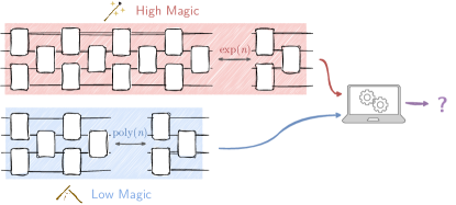
Figure 1: The ‘pseudomagic’ state ensembles discussed in this work are computationally indistinguishable from highly magical states produced by chaotic dynamics (i.e., Haar random states).

Definition 1 (Pseudomagic).

Let $\mathcal{M}$ be a magic measure. A pseudomagic pair with gap $f(n)$ vs. $g(n)$ (where $f(n)>g(n)$) consists of two state ensembles:

1. a ‘high magic’ ensemble of $n$-qubit quantum states $\{|\psi_{k_{1}}\rangle\}$ such that $\mathcal{M}({\psi_{k_{1}}})=f(n)$ with high probability over $k_{1}$, and

2. a ‘low magic’ ensemble of $n$-qubit quantum states $\{|\phi_{k_{2}}\rangle\}$ such that $\mathcal{M}({\phi_{k_{2}}})=g(n)$ with high probability over $k_{2}$,

such that the two ensembles are computationally indistinguishable, even when given polynomially many copies of the state. That is, for all polynomial time quantum algorithms $\mathcal{A}$ given $t=O(\operatorname{poly}n)$ copies of a state,

$$\left|{\mathsf{Pr}}[\mathcal{A}(|\psi_{k_{1}}\rangle^{\otimes t})=1]-{\mathsf{Pr}}[\mathcal{A}(|\phi_{k_{2}}\rangle^{\otimes t})=1]\right|=o\left(\frac{1}{\operatorname{poly}n}\right)$$ (1)

with high probability over $k_{1}$ and $k_{2}$.

Qualitatively, states from the ensemble $\{|\psi_{k_{2}}\rangle\}$ mimic much more ‘magical’ states to any algorithm that runs in polynomial time, even though they themselves are ‘low magic’. In the rest of this work we use stabilizer Rényi entropy as our magic measure, given by

$$M_{\alpha}({\psi})=\frac{1}{1-\alpha}\log\frac{1}{d}\sum_{P\in\mathbb{P}_{n}}\mathrm{tr}^{2\alpha}(P\psi),$$ (2)

although this choice of magic measure is not unique.

We turn to $f(n)$, the high-magic ensemble. A prototypical choice for such an ensemble is the ensemble of Haar-random states. As we show in SM II.2, Haar-random states have stabilizer entropy $\Theta(n)$ with overwhelming probability, which is to say that they achieve maximal magic . In this paper, unless otherwise specified, we will let the high-magic ensemble be the Haar-random states, and reserve the term ‘pseudomagic ensemble’ for the low-magic ensemble, which is often of more interest.

Combining the ‘computational indistinguishability’ property with the properties of stabilizer Rényi entropy, we compute the minimal possible magic for the pseudomagic ensemble. Throughout this work, we frequently employ the Bachmann-Landau notation for asymptotics . We show that $g(n)$, the magic of the low-magic ensemble, can be no smaller than $\omega(\log n)$:

Lemma 1 (Bound to stabilizer entropies).

Let $\mathcal{E}$ be an ensemble of pseudomagic states. Then the $\alpha$-Rényi stabilizer entropies obey $M_{\alpha}({\psi})=\omega(\log n)$, with high probability over the choice of $|\psi\rangle\in\mathcal{E}$.

Proof.

Stabilizer entropies can be measured efficiently. We leverage this fact to make a distinguisher that can efficiently distinguish states whose stabilizer entropies are $O(\log n)$ from states whose stabilizer entropies are $\Omega(n)$, thus contradicting the assumption that these states are pseudomagic. See SM II.1 for a detailed proof. ∎

Construction of pseudomagic ensembles. Now, we give a construction of pseudomagic states that are also pseudorandom [47] (i.e., computationally indistinguishable from Haar random states), and that saturate the lower bound in Lemma 1:

Definition 2 (Subset phase states [31]).

For a pseudorandom function $f:\{0,1\}^{n}\to\{0,1\}$ and $S\subseteq\{0,1\}^{n}$ a pseudorandom subset, define the associated subset phase state vector as

$$|\psi_{f,S}\rangle=\frac{1}{\sqrt{|S|}}\sum_{x\in S}(-1)^{f(x)}|x\rangle.$$ (3)

Theorem 1 (Subset phase states display pseudomagic).

For any $\omega(\log n)<k\leq n$, there exists a family of pseudorandom functions $f$ such that the state ensemble $\mathcal{E}=\{|\psi_{f,S}\rangle\}$ corresponding to $S$ of size $2^{k}$ has magic $M_{\alpha}({\psi_{f,S}})=O(k)$. For $\alpha\leq 2$, this bound is tight: $M_{\alpha}({\psi_{f,S}})=\Theta(k)$.

Moreover, $\mathcal{E}$ is computationally indistinguishable from the ‘high magic’ ensemble of Haar random states, i.e. they are pseudorandom; furthermore, for any two families of pseudorandom functions $f_{1},f_{2}$ and any two families of pseudorandom subsets $S_{1},S_{2}$ such that $\omega(\log n)<\log(|S_{1}|)\leq\log(|S_{2}|)\leq n$, $\{|\psi_{f_{1},S_{1}}\rangle\}$ and $\{|\psi_{f_{2},S_{2}}\rangle\}$ are computationally indistinguishable from each other.

Proof.

We show in Lemma 5 of SM II.2 that any subset phase state vector $|\psi_{f,S}\rangle$ satisfies

$$M_{0}({\psi_{f,S}})\leq 2\log\left|S\right|$$ (4)

and then use the fact that $M_{\alpha}({\psi})\geq M_{\alpha^{\prime}}({\psi})$ for $\alpha^{\prime}>\alpha$. The tightness of the bound for $\alpha\leq 2$ is shown in SM II.3. The ‘moreover’ part follows from Ref. [31]. The computational indistinguishability of subset phase state ensembles follows from transitivity of computational indistinguishability (see Lemma 9 in SM III), choosing $\mathcal{E}_{2}$ to be the Haar-random ensemble. ∎

It is natural to ask if, besides the stabilizer Rényi entropy, other magic measures (see Table 1) can be used to define pseudomagic. In SM II.4, we show that both the $\alpha$-stabilizer entropies $M_{\alpha}(\psi)$ and the log-robustness of magic $\mathcal{R}(\psi)$ are measures of pseudomagic with gap $\Theta(n)$ vs. $\Theta(\operatorname{poly}\log n)$. As a corollary, we have a sufficient condition for a magic measure to be a good measure for defining pseudomagic:

Corollary 1 (Good magic monotones for large-gap pseudomagic).

For any magic monotone $\mathcal{M}$, if there exists an $\alpha$ such that $\Omega(M_{\alpha}(\psi))\leq\mathcal{M}(\psi)\leq O(\mathcal{R}(\psi))$ for pure states $\psi$, then $\mathcal{M}$ is also a measure of pseudomagic with gap $\Theta(n)$ vs. $O(\operatorname{poly}\log n)$. Moreover, if $\alpha\leq 2$, the gap tightens to $\Theta(n)$ vs. $\Theta(\operatorname{poly}\log n)$.

In SM II.5, we use this corollary to show that the magic monotones $\mathcal{M}=\mathcal{F}_{\textrm{stab}}(\psi),\xi(\psi),D_{\max}(\psi)$, as defined in Table 1, are measures of pseudomagic with gap $\Theta(n)$ vs. $\Theta(\operatorname{poly}\log n)$. Conversely, some magic measures do not display this large pseudomagic gap when we choose the high magic ensemble to be Haar random states. In SM II.6, we show that the stabilizer nullity [48], which counts the number of preserved stabilizer symmetries in quantum states, falls into this latter camp: it is maximal with overwhelming probability for pseudorandom states (i.e., any states that are indistinguishable from Haar random), and therefore our machinery in this paper does work to define pseudomagic for such magic measures.

The astute reader may notice that the states that display pseudomagic are the same states that display pseudoentanglement [31]. Given the long history of resource theories centered on these two quantities, it is natural to wonder if the existence of pseudomagical ensembles is in some way implied by the existence of pseudoentangled ensembles. In the following theorem, we answer this question in the negative: starting from the subset phase states, magic and entanglement can be boosted to their maximal value independently of the other by applying efficient unitaries. Furthermore, the pseudorandomness is preserved even after these transformations (see Fig. 2). This suggests that neither pseudomagic nor pseudoentanglement is a generic feature of pseudorandom ensembles.

Theorem 2 (Pseudomagic and pseudoentanglement are independent properties).

For the ensemble of subset phase states $\mathcal{E}=\{|\psi_{f,S}\rangle\}$, there exists

1. a Clifford $U^{*}\in\mathcal{C}_{n}$ such that $\{U^{*}|\psi_{f,S}\rangle\}$ has maximal (i.e., volume law) entanglement across superpolynomially many cuts and yet retains the same magic as $\mathcal{E}_{f,S}$;

2. a product of local unitaries $U^{*}=\bigotimes_{i=1}^{n}U_{i}^{*}$ such that $\{U^{*}|\psi_{f,S}\rangle\}$ has maximal (i.e., $\Theta(n)$) magic and yet retains the same entanglement as $\mathcal{E}$.

3. a unitary $U^{*}$ with a polynomial depth brickwork circuit such that $\{U^{*}|\psi_{f,S}\rangle\}$ has simultaneously maximal entanglement and maximal magic.

Moreover, all these unitaries preserve the pseudorandomness of the original ensemble.

Proof.

For (a), we show that for any state $|\psi\rangle$, when $U$ is sampled uniformly at random from the Clifford group, $U|\psi\rangle$ has unchanged magic, but exhibits volume law entanglement. For (b) and (c), we follow a similar strategy by averaging over products of independent Haar random single qubit unitaries and random brickwork circuits, respectively. Furthermore, our statements in (a) and (c) hold for any pseudorandom ensemble $\mathcal{E}$, not just the subset phase states. The detailed proofs are in SM IV. ∎

In fact, these results can be strengthened. We can guarantee that there is a pseudorandom ensemble displaying any value of average entanglement and any value of average magic within the range allowed by the definition of pseudomagic and pseudoentanglement:

Theorem 3 (Independence theorem).

For any $\Omega(\operatorname{poly}\log n)\leq g(n),h(n)\leq O(n)$, we can construct pseudorandom ensembles that have average entanglement $g(n)$ across exponentially many cuts $(A_{i},B_{i})$ that are linear in system size, i.e.

$$\mathbb{E}_{B_{i}}\mathbb{E}_{|\psi\rangle\sim\mathcal{E}}\left[S(\mathrm{tr}_{B_{i}}(|\psi\rangle\!\langle\psi|))\right]=\Theta(g(n))$$ (5)

and average magic $h(n)$, i.e.

$$\mathbb{E}_{|\psi\rangle\sim\mathcal{E}_{U}}[M_{\alpha}(\psi)]=\Theta(h(n))$$ (6)

This theorem is proven in SM IV. The larger range of achievable entanglement and magic as compared to Theorem 2 turns out to be crucial for strengthening our statements for some of our later applications. In the rest of this work, we discuss the implications of pseudomagic in the fields of quantum chaos, quantum cryptography, black-box magic state distillation and testing non-stabilizerness.

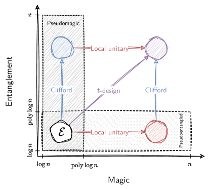
Figure 2: The pseudorandom ensemble of states $\mathcal{E}$ (subset phase states) we consider in this work exhibit both pseudomagic and pseudoentanglement. However, we show that we can efficiently convert between the four entanglement/magic quadrants via Clifford unitaries, local unitaries, and approximate $t$-designs.

Implications to quantum chaos. Having defined the notion of pseudomagic, we now use it to address some important aspects of quantum chaos theory. One way of defining a quantum chaotic unitary evolution $U$ is to say that it is chaotic if it attains the Haar value for its $2k$-point out-of-time-order correlators (OTOCs) [49, 50]. These OTOCs are denoted by $C_{2k}$ and defined as

$$C_{2k}(U)\coloneqq\frac{1}{d}\mathrm{tr}(\tilde{P}_{1}Q_{1}\tilde{P}_{2}Q_{2}\cdots\tilde{P}_{k}Q_{k}),$$ (7)

where $P_{i}$ and $Q_{i}$ are non-identity Pauli operators for $i=1,\ldots,k$ and $\tilde{P}_{i}\coloneqq U^{{\dagger}}P_{i}U$. To be precise, $U$ is chaotic if $C_{2k}(U)=\tilde{O}(C_{2k}(U_{\operatorname{Haar}}))$, where $\tilde{O}$ stands for an irrelevant polynomial overhead. Indeed, typically $C_{2k}(U_{\operatorname{Haar}})=O(\exp(-\gamma n))$ with $\gamma$ depending on the particular choice of the correlator $C_{2k}$ [49].

The resource theory of magic is closely linked to the theory of quantum chaos [51, 52, 53]. Indeed, it has been shown that any unitary which exhibits chaotic behavior for its OTOCs must contain $\Theta(n)$ non-Clifford gates [54, 55]. The more general question of how much non-stabilizerness (as measured by the stabilizer entropy) is necessary to drive a quantum system towards quantum chaos has been addressed in Ref. [27], where it was demonstrated that a unitary $U$ can exhibit chaos only if it has maximal nonstabilizer power (i.e., when applied to stabilizer state vectors $|\sigma\rangle$, it produces $U|\sigma\rangle$ with $\Theta(n)$ magic). Consequently, the mere existence of pseudomagic states that are also pseudorandom (i.e., subset phase states), suggests the existence of non-chaotic unitaries that nonetheless generate states indistinguishable from Haar random states. More precisely, in the following theorem, we establish that such states must be generated by a non-chaotic unitary evolution that exhibits exponentially separated OTOCs from the typical Haar value.

Theorem 4 (Hidden quantum chaos).

Let $\mathcal{E}$ be an ensemble of pseudomagic states that is also pseudorandom. Let $|\psi\rangle\in\mathcal{E}$ and let $U$ such that $|\psi\rangle=U|0\rangle^{\otimes n}$. The $2k$-point OTOCs of $U$ (for $k\geq 4$) are exponentially separated from the Haar value,

$$C_{2k}(U)=\Omega(\exp(n)C_{2k}(U_{\operatorname{Haar}})).$$ (8)

Therefore, although it generates a state that is on-average computationally indistinguishable from Haar-random, $U$ cannot be considered chaotic.

The proof of this can be found in SM V. Theorem 4 has a curious implication: no physical observer, that is naturally subject to computational limits, can distinguish chaotic from non-chaotic evolution solely based on the observed resultant state (see Fig. 1). This observation prompts the broader question: do there exist non-chaotic unitaries indistinguishable from Haar random unitaries? Exploring this remains an intriguing subject for future research.

Implications to quantum cryptography. An essential primitive for classical cryptography is the concept of a one-way function (OWF), which is a function which is efficient to evaluate but hard to invert. However, the story is vastly different in the quantum world: OWFs are unnecessary for some quantum cryptographic constructions to hold [56, 57]. This leads naturally to a question of whether there is an indespensible primitive for quantum cryptography that serves a similar role to OWFs for classical cryptography. In Ref. [33], the authors introduce EFI pairs as this quantum analogue and show that it is necessary for many secure quantum cryptographic schemes, including bit commitment [58, 59], oblivious transfer [60, 61], multiparty quantum computation [62], and zero knowledge proofs [63]. EFI pairs are state ensembles generated by efficient circuits that are statistically far but computationally indistinguishable. In light of the proposed significance of EFIs, we show the following theorem.

Theorem 5 (Cryptographic implications).

Consider an ensemble of efficiently preparable pseudomagic states that have stabilizer entropy $M_{1}=\Theta(g(n))$ with high probability, where $g(n)$ is tunable in the range $\omega(\log n)$ and $O(n)$. Then, the pseudomagic ensemble, along with the high magic ensemble, forms an EFI pair.

For a proof, see SM VI. Crucially, Theorem 5 holds even in a world without quantum-secure OWFs: it says that the bare existence of pseudomagic states with tunable stabilizer entropy implies the existence of EFI pairs and the world of cryptographic applications they unlock. This strengthens the case that EFI pairs are a more fundamental primitive for quantum cryptography than OWFs.

No efficient black-box magic-state distillation. Several architectures for universal fault-tolerant quantum computing rely on applying stabilizer operations to carefully prepare resource states called magic states [64, 25, 65, 66]. An example is the canonical magic state vector $|T\rangle=|0\rangle+e^{i\pi/4}|1\rangle$, which when provided as an input to auxiliary qubits, enables $T$-gate implementation using only stabilizer operations. However, not all nonstabilizer states are useful for implementing non-Clifford gates [48]. This motivates the question, can we develop efficient stabilizer protocols that can transform generic nonstabilizer states $\rho$ into specific and useful nonstabilizer states, such as $|T\rangle$? In line with the spirit of analogous tasks for entanglement resource theory [67, 68], we term this task black-box magic-state distillation.

Pseudomagic provides a complementary perspective to magic resource theory in determining the distillability limits of magic states. Prior to this work, it was already known that magic monotones $\mathcal{M}$ are nonincreasing under stabilizer operations. Therefore, if we have a target magic state $|B\rangle\langle B|$ and a generic input state $\rho$, magic resource theory tells us that if $\mathcal{M}(\rho)<\mathcal{M}(|B\rangle\langle B|)$, no stabilizer protocol can transform $\rho\to|B\rangle\langle B|$. Conversely, when $\mathcal{M}(\rho)\geq\mathcal{M}(|B\rangle\langle B|)$, a stabilizer protocol cannot be ruled out from resource theory considerations alone. However, it could be challenging to find or implement such a protocol in practice. Our pseudomagic construction now establishes when such protocols are computationally inefficient:

Theorem 6 (Black-box magic state distillation).

Given a magic monotone $\mathcal{M}$ such that $\Omega(M_{\alpha}(\psi))\leq\mathcal{M}(\psi)\leq O(\mathcal{R}(\psi))$ for all pure states $\psi$, any efficient stabilizer protocol that synthesizes a state $|B\rangle\langle B|$ from an arbitrary (potentially mixed) input state $\rho$ requires

$$\Omega\left(\frac{\mathcal{M}(|B\rangle\langle B|)}{\log^{1+c}\mathcal{M}(\rho)}\right)$$ (9)

copies of $\rho$, for any constant $c>0$.

The proof of this can be found in SM VII. In words, the meaning of this theorem is as follows. A naive lower bound from resource theory considerations would say that we require $\Omega({\mathcal{M}(|B\rangle\langle B|)}/{\mathcal{M}(\rho)})$ copies of $\rho$ to synthesize $|B\rangle\langle B|$. This assumes that we can freely convert from magic in the input state to magic in the output state. However, once we take into account the computational efficiency of our synthesization protocol, Theorem 6 intuitively means that if we do not know what the input state is, the ‘value’ of the magic in the input state is reduced logarithmically. To illustrate this, consider a concrete example. Assume we have a generic resource state vector $|\psi\rangle$ with $\mathcal{M}({\psi})=an$ ($a<1$). In this case, the naive bounds tell us that we can distill at most $r=O(an)$ canonical magic state vectors $|T\rangle$, since $\mathcal{M}(|T\rangle\langle T|^{\otimes r})\propto r$. However, Theorem 6 imposes a much stricter bound; if our synthesis protocol is efficient, it can synthesize at most $r=O(\log^{1+c}(an))$ copies of $|T\rangle$. We reiterate that Theorem 6 is valid for a arbitrary input state (pure or mixed) $\rho$. This fact, and a number of insights into mixed state protocols, is further developed in SM VII.

Magic does not help in entanglement distillation and entanglement does not help magic distillation. In Theorem 3, we have already seen an independence theorem that hints that magic and entanglement are two very different resources. In this section, we crystallize this intuition into strengthenings of our Theorems 6 and 9 as well as many of the applications in Ref. [31]: we show that prior knowledge of the magic of the input states does not make entanglement distillation more efficient, nor does prior knowledge of entanglement ameliorate the situation with magic state distillation.

Theorem 6 and Proposition 3.1 of Ref. [31] (on lower bounds to entanglement distillation) are similar in spirit: they demonstrate that the resource-theoretic maximum of the number of distillable EPR pairs/magic states is a gross overestimate of what is achievable by any computationally efficient algorithm that is agnostic to its input state – that is, any algorithm that should work on any input state they are given. But a critic could argue that this last assumption is unjustified – many magic state or entanglement distillation protocols are hand-crafted to work on particular classes of input states [1, 69]. Do our lower bounds still hold up, then, if we knew something about the state we started with? For example, if we knew that the input state is drawn from a class of states known to have high magic, does that allow for computationally efficient entanglement distillation algorithms, or could one, as Ref. [70] proposed, distill magic from highly entangled states – if we limit ourselves to computationally efficient distillers? We use our independence theorem 3 to answer in the negative:

Theorem 7 (High magic doesn’t help entanglement distillation).

Consider an entanglement distillation protocol that distills EPR pairs from states drawn from an ensemble $\{\psi_{k}\}$. Even if we are guaranteed that the states $\psi_{k}$ have magic $\Theta(n)$ with overwhelming probability, the protocol can distill at most $O(\log^{1+c}S(\rho))$ Bell pairs with high probability, where $S(\rho)$ is the von Neumann entanglement entropy across a bipartition of the system that is linear in $n$.

Proof.

Assume the contrapositive. Then, following a similar argument as [31], one could use this entanglement distillation protocol to distinguish between a Haar random state—which has both magic and entanglement scaling as $\Theta(n)$ with overwhelming probability—and a pseudorandom ensemble of the type explicitly constructed in the proof of Theorem 3—which can have magic $\Theta(n)$ with overwhelming probability but entanglement $\operatorname{poly}\log n$. The distinguisher just counts the number of EPR pairs produced. ∎

An identical strengthening of the black-box magic state distillation protocol in Theorem 6 is also possible, using a similar proof technique.

Theorem 8 (High entanglement doesn’t help magic distillation).

Consider a magic distillation protocol that distills copies of a target state $|B\rangle$ from states drawn from an ensemble $\{\psi_{k}\}$. Even if we are guaranteed that, with overwhelming probability, the states $\psi_{k}$ have entanglement $\Theta(n)$ across exponentially many cuts $(A_{i},B_{i})$, where the size of both cuts have size $\Omega(n)$, the number of required copies of the input state is still lower bounded by the constraints given in Eq. 9.

We note that it is possible to generalize Theorems 7 and 8 to states that display on average any amount of magic/entanglement bounded between $\omega(\log n)$ and $n$, using our Independence Theorem (Theorem 3). More concretely, this pair of theorems implies that we cannot distill entanglement from low Schmidt-rank states, nor magic from states prepared by geometrically local random quantum circuits of restricted depth, which are believed to be valid pseudorandom quantum states and finds use in quantum advantage demonstrations [71, 72], or those prepared by generic local Hamiltonians acting on a fixed reference state for restricted time, which may be of interest in condensed matter physics [73]. The entanglement and magic of these states (in expectation) can be tuned by varying the depth of the circuit or the time of the evolution.

Testing non-stabilizerness. A property test is an algorithm that checks whether a given unknown state has a particular property or not. We now focus on property testers for non-stabilizerness and present a theorem that characterizes the requirements for any such tester.

Theorem 9 (Testing non-stabilizerness).

Given $K$ copies of a state $|\psi\rangle$ and two threshold values $m,M\in[0,n]$ with $m<M$, a tester for a magic measure $\mathcal{M}$ determines whether $\mathcal{M}({\psi})\not\in[m,M]$ with probability $\geq 2/3$. Any tester for the stabilizer entropy $M_{\alpha}$, with $M<{n}/({4\alpha})$, requires $K=\Omega\left(2^{\frac{m}{4+c}}\right)$ copies, for any constant $c>0$.

An immediate corollary is that any property tester for any monotone $\mathcal{M}$ lower bounded by $sM_{\alpha}$ requires at least $K=\Omega(2^{\frac{m/s}{4+c}})$ copies. In particular, the statement is valid for any magic measure in Table 1. The proof of Theorem 9 as well as the corollary is to be found in SM VIII. We remark that in a similar fashion to Theorems 7 and 8, the above theorem can be strengthened to hold against non-stabilizerness testers designed for classes of input states with bounded entanglement between $\omega(\log(n))$ and $n$. We may similarly strengthen the property testing lower bounds in Section 3 of Ref. [31] to hold for input states with bounded magic.

Experimental feasibility. We conclude by proposing a potential method that uses Rydberg arrays to realize subset phase state vectors $|\psi_{f,S}\rangle$ – which, as we remind the reader, constitute pseudorandom ensembles that display both pseudomagic and pseudoentanglement. Given the plethora of applications of pseudomagic discussed above, an experimental realization of pseudomagic states could hold significant scientific value. Furthermore, this illustrates that these states, despite displaying remarkable properties, are not merely artificial theoretical constructions: they can be implemented in the laboratory.

The first step of our construction provides a concrete implementation for the black-box oracles $f$ described in Ref. [31]. We first assume $\left|S\right|=2^{k}$ for some integer $k\leq n$. For any function $f:\{0,1\}^{k}\to\{0,1\}$, one can associate a hypergraph over $k$ sites with hyperedges $E$ such that $f(x)=\sum_{\{i_{1},\ldots,i_{m}\}\in E}\prod_{\alpha=1}^{m}x_{i_{\alpha}}$. Then, it turns out that we can attach the appropriate phases to the bit string states by simply applying multi-qubit CZ gates on sites are connected by hyperedges [74] as

$$\prod_{\{i_{1},\ldots,i_{m}\}\in E}C^{m-1}Z_{i_{1}\ldots i_{m}}|+\rangle^{\otimes k}=\sum_{x\in\{0,1\}^{k}}(-1)^{f(x)}|x\rangle.$$ (10)

Finally, by concatenating $|0\rangle^{\otimes(n-k)}$ and applying a pseudorandom permutation of computational basis states [31], we arrive at the desired $|\psi_{f,S}\rangle$.

This protocol has quasipolynomial time complexity, as the hypergraph representation of $f$ can have a quasipolynomial number of edges, so we anticipate that for near-term qubit counts $n$, the construction of these states will be feasible. In particular, neutral-atom platforms such as Rydberg arrays, are very well-suited for implementing this construction for two key reasons. First, these platforms offer the advantage of being able to quickly move qubits around, allowing for the realization of the required hypergraph connectivity. Secondly, these platforms natively support the implementation of multi-qubit CZ gates [75]. This streamlines the creation of subset phase state vectors $|\psi_{f,S}\rangle$ using a native set of gates, making the implementation straightforward and noise-resilient.

Conclusions and outlook. In this work, we have introduced the concept of pseudomagic states in quantum computation, providing an insightful expansion of the resource theory of magic. We first established the theoretical foundation for pseudomagic states. At the core of the this framework lies the stabilizer entropy, which is uniquely distinguished among various magic measures (see Table 1) as it does not require an unwieldy minimization procedure to be evaluated either theoretically or experimentally. However, we note that the stabilizer entropy differs from other magic measures in that for $\alpha<2$, there may exist exotic counterexamples to the monotonicity of stabilizer entropy [36], and that the null set for mixed states differs from the usual null set for magic-state distillation [27]. As such, for tasks such as magic-state distillation, other magic measures are more natural tools. Nevertheless, the stabilizer entropy has proven to be a fundamental tool for defining and exploring pseudomagic. For instance, a key property we make frequent use of, especially when developing a general framework for pseudomagic, was that several other popular magic monotones are lower bounded by the stabilizer entropy, hence qualified as useful pseudomagic measures.

Having laid a general framework for pseudomagic, we have then investigated the implications of this construction for a variety of questions in quantum chaos theory, quantum cryptography, magic state distillation problems and property testing. In particular, the construction of pseudomagic states has remarkable implications for quantum chaos: it proves the existence of states, preparable with a non-chaotic unitary, that nevertheless appear to have been generated by a chaotic one. This has led us to conclude that a physical observer, who is surely subject to computational constraints, cannot conclusively determine whether a process is chaotic merely by looking at the states generated by that process. More general questions concerning the existence of pseudorandom unitaries [76] and its consequence for quantum chaos theory will be the subject of future research. Another exciting avenue to explore is the implication that pseudomagic has for many-body physics, particularly in light of the recent extensive studies of magic-state resource theory [77, 78, 79, 80, 81, 82, 83, 84] and quantum complexity in many-body systems [85].

Yet, as previously suggested, the significance of computational indistinguishability extends beyond investigating quantum resource theories such as magic and entanglement. It introduces a unique perspective into the quantum realm of many particles, transforming the laboratory from a mere verifier of quantum theories into an integral part of the theory itself, where the limitations of observers assume a central role.

Acknowledgements. The authors thank Anurag Anshu, J. Pablo Bonilla, Matthias Caro, Bill Fefferman, Jonas Haferkamp, Marcel Hinsche, Marios Ioannou, Nazlı Uğur Köylüoğlu, Salvatore F. E. Oliviero, Kunal Sharma, Ryan Sweke for insightful discussions, We also thank William Kretschmer for suggesting the proof of Theorem 5, and Joseph Slote for first using the term “pseudomagic” and discussing different magic measures. We thank the DFG (CRC 183, FOR 2724), the BMBF (Hybrid, RealistiQ, QSolid), and the Munich Quantum Valley (K-8) for funding. SFY would like to thank the NSF for funding via the Cornell HDR institute and the CUA PFC.

Supplemental Material

In this supplemental material, we provide proofs, additional details supporting the claims in the main text, as well as additional applications of pseudomagic.

Supplemental Material I:  Preliminaries

There are many ways to quantify magic. In this work, we consider only monotones; that is, those measures that satisfy the following properties:

Definition 3 (Magic monotone).

A magic monotone is a scalar function on quantum states, that has the following properties:

• $\mathcal{M}(\sigma)=0$ if and only if $|\sigma\rangle\in\Sigma$,

• $\mathcal{M}(\mathcal{S}(\psi))\leq\mathcal{M}(\psi)$ for every stabilizer operation $\mathcal{S}$.

The magic measures $\mathcal{M}$ we consider in our study obey $(i)$ sub-additivity $\mathcal{M}({\psi}\otimes{\phi})\leq\mathcal{M}({\psi})+\mathcal{M}({\phi})$, $(ii)$ are bounded $0\leq\mathcal{M}\leq n+o(1)$ , which will be assumed throughout this work.

I.1 Properties of stabilizer Rényi entropies

In this work we will focus on the measure of $\alpha$-stabilizer entropies. Let us now introduce this family of measures formally. We observe that given a $n$-qubit (pure or mixed) state $\psi$, we can define the probability distribution

$$\Xi_{\psi}\coloneqq\{d^{-1}\mathrm{tr}^{2}(P\psi)\operatorname{Pur}^{-1}(\psi)\mid P\in\mathbb{P}_{n}\},$$ (S1)

where $\mathbb{P}_{n}$ is the Pauli group on $n$ qubits and $\operatorname{Pur}(\psi)\coloneqq\mathrm{tr}(\psi^{2})$ its purity. The stabilizer entropy $M_{\alpha}$ is defined as (for every $0\leq\alpha<\infty$)

$$M_{\alpha}(\psi)\coloneqq S_{\alpha}(\Xi_{\psi})+S_{2}(\psi)-\log d,$$ (S2)

where $S_{\alpha}(\Xi_{\psi})$ is the classical $\alpha$-Rényi entropy of the probability distribution in Eq. S1, while $S_{2}(\psi)\coloneqq-\log\operatorname{Pur}(\psi)$ is the log-purity of $\psi$. To be concrete, we list three explicit expressions for $M_{\alpha}$ for common choices of $\alpha$ (we also assume $\psi$ is pure for simplicity),

$$M_{\alpha}(\psi)=\begin{cases}\log(\left|\{P\in\mathbb{P}_{n}\mid\mathrm{tr}(P\psi)\neq 0\}\right|)-\log d&\text{for $\alpha=0$},\\ -\sum_{P}\frac{\mathrm{tr}^{2}(P\psi)}{d}\log\mathrm{tr}^{2}(P\psi)&\text{for $\alpha=1$},\\ -\log(\sum_{P}\frac{\mathrm{tr}^{4}(P\psi)}{d})&\text{for $\alpha=2$.}\end{cases}$$ (S3)

The first two cases of $\alpha=0$ and $1$ are manifestly different from the definition $M_{\alpha}({\psi})=\frac{1}{1-\alpha}\log\frac{1}{d}\sum_{P}\mathrm{tr}^{2\alpha}(P\psi)$ presented in Eq. 2. Despite the formal difference, the $\alpha=0$ and $1$ cases are not discontinuous exceptions to the definition in Eq. 2. Rather, they follow from the definition of the classical Rényi entropies: $\lim_{\alpha\to 0}S_{\alpha}(\Xi_{\psi})=\log\left|\text{supp}\ \Xi_{\psi}\right|$, where $\text{supp}\ \Xi_{\psi}$ is the support of the distribution $\Xi_{\psi}$. Similarly, $\lim_{\alpha\to 1}S_{\alpha}(\Xi_{\psi})=-\sum_{P}\Xi_{\psi}(P)\log(\Xi_{\psi}(P))$ (i.e., the Shannon entropy of $\Xi_{\psi}$). Therefore, despite the fact that the cases $\alpha=0$ and $\alpha=1$ may superficially seem to be special exceptions, in what follows (unless otherwise specified), we will be studying $M_{\alpha}$ for any $\alpha$.

Let us list important properties of the $\alpha$-stabilizer entropies.

• $M_{\alpha}(\sigma)=0$ if and only if $\psi=\sum_{P\in G_{\sigma}}\phi_{P}P$, where $G_{\sigma}$ is a commuting subgroup of $\mathbb{P}$ and $\phi_{P}\in\{\pm 1\}$. Notice that $\sigma$ is pure if and only if $\left|G_{\sigma}\right|=2^{n}$. The zeros of the stabilizer entropy (i.e., the states $\psi$ for which $M_{\alpha}(\psi)=0$) coincides with the set of pure stabilizer state plus mixed stabilizer states defined above. However, $M_{\alpha}(\psi)>0$ when $\psi$ is a convex combination of stabilizer states: $\psi=\sum_{\sigma\in\Sigma}p_{\sigma}|\sigma\rangle\!\langle\sigma|$, where $p_{\sigma}\geq 0$. Notice that the zeros of the stabilizer entropy do not coincide with the zeros of other magic measures for mixed states.

• For every Clifford unitary operator $C$, then $M_{\alpha}(C^{{\dagger}}\psi C)=M_{\alpha}(\psi)$;

• $0\leq M_{\alpha}(\psi)<n$, where the upper bound is a strict inequality.

• They feature a hierarchy: $M_{\alpha}(\psi)<M_{\alpha^{\prime}}(\psi)$ for any $\psi$ if $\alpha>\alpha^{\prime}$.

• They are additive: $M_{\alpha}(\psi\otimes\phi)=M_{\alpha}(\psi)+M_{\alpha}(\phi)$.

• For pure states ${\psi}$, they lower bound the stabilizer nullity: $M_{\alpha}({\psi})\leq\nu({\psi})$.

• For pure states and $\alpha>1/2$, they lower bound the robustness of magic $M_{\alpha}({\psi})<2\mathcal{R}({\psi})$ [87].

• For pure states and $\alpha>1$, they lower bound the stabilizer fidelity: $M_{\alpha}({\psi})<\frac{2\alpha}{\alpha-1}\mathcal{F}_{\textrm{stab}}({\psi})$ [36].

• Defining $T$-count as smallest number $t(\psi)$ of $T$-gates used to prepare the state vector $|\psi\rangle$ from a stabilizer state, the stabilizer entropies lower bound the $T$-count: $M_{\alpha}({\psi})\leq t(\psi)$.

• Using the replica trick, when $\alpha$ is an integer greater than 1, we can also write $M_{\alpha}$ as follows:

  $$M_{\alpha}({\psi})=\frac{1}{1-\alpha}\log\mathrm{tr}(\Pi^{(2\alpha)}\psi^{\otimes 2\alpha}),$$ (S4)

  with $\Pi^{(2\alpha)}\coloneqq d^{-1}\sum_{P\in\mathbb{P}_{n}}P^{\otimes 2\alpha}$ being a Hermitian operator. Thanks to this property, stabilizer entropies can be measured on quantum computers with both single copy protocols such as randomized measurements [88], as well as multi-copy protocols [38, 36].

I.2 A remark on the role of stabilizer entropy in defining pseudomagic

Considering the properties of magic monotones highlighted in the main text, it is relevant to note that stabilizer entropies for $\alpha<2$ do not exhibit the property of being non-increasing under conditioned Clifford unitaries, as demonstrated in Ref. [36]. Consequently, they cannot be classified as genuine magic monotones. Regarding the case where $\alpha\geq 2$, the question of whether they remain non-decreasing under conditioned Clifford unitaries remains an open question. Given that, we are in good position to stress the true role of stabilizer entropy in defining pseudomagic in general, and for problems strictly related to magic-state resource theory.

The use of stabilizer entropy for pseudomagic is of utmost importance for quantum highlights in the context of quantum chaos theory (Theorem 4) (given its strict relationship to OTOCs) and in quantum cryptographic implications (Thereom 5) (thanks to the Fannes inequality for $M_{1}$). However, in defining pseudomagic, a genuine magic monotone can be often desirable. Examples of this king are Theorem 6 where we place a constraint on magic-state distillation protocols or Theorem 9 where we want to test magic given a specific monotone $\mathcal{M}$. In regards of these tasks, the role of stabilizer entropy is to provide a tight pseudomagic gap for all the genuine monotones. To be more concrete, all the other monotones, except for stabilizer entropy, involve a minimization procedure that renders them computationally and experimentally intractable to measure. Consequently, they are unsuitable for proving a pseudomagic gap, which asks for measurement using multiple copies to provide the lower bound $\omega(\log n)$ for pseudomagic ensembles. Thanks to the fact that stabilizer entropy $(i)$ provides a lower bound for all the other magic monotones and $(ii)$ can be experimentally measured, we are able to demonstrate the existence of states with an extensive and tight gap of $\log n$ versus $n$ in magic, which holds true for all the monotones, both genuine and non-genuine, discussed in this paper. This fact is reflected by Corollary 1.

I.3 Pseudorandom states

The other key idea we use throughout this work is the notion of pseudorandom states, which are ensembles of states that are disguised as Haar random.

Definition 4 (Pseudorandom states [47]).

An ensemble of $n$-qubit quantum states $\left\{|\psi_{k}\rangle\mid k=1,\ldots,2^{m}\right\}$ (where $m\in\mathbb{N}$) is said to be pseudorandom, if:

• Given $k$, the corresponding $|\psi_{k}\rangle$ is preparable in polynomial time.

• For any efficient quantum algorithm $\mathcal{A}$,

  $$\left|{\mathsf{Pr}}[\mathcal{A}\big{(}|\psi_{k}\rangle^{\otimes\operatorname{poly}(n)}\big{)}=1]-{\mathsf{Pr}}[\mathcal{A}\big{(}|\phi\rangle^{\otimes\operatorname{poly}(n)}\big{)}=1]\right|={\mathsf{negl}}(n),$$ (S5)

  with high probability for $k\sim\textnormal{Uniform}(2^{m})$ and $\phi\sim\operatorname{Haar}$. In other words, polynomially many copies of $|\psi_{k}\rangle$ are computationally indistinguishable from polynomially many copies of a Haar random state.

The subset phase states are a class of states that are capable of satisfying Definition 4 under certain settings. Specifically, they are ensembles of states

$$|\psi_{f,S}\rangle=\frac{1}{\sqrt{\left|S\right|}}\sum_{x\in S}(-1)^{f(x)}|x\rangle.$$ (S6)

indexed by a function $f:\{0,1\}^{n}\to\{0,1\}$ and subsets $S\subseteq\{0,1\}^{n}$. If $\left|S\right|=2^{\omega(\log n)}$ and $f$ is a truly random function, then the subset phase states are statistically indistinguishable from the Haar random states (i.e., polynomially many copies of $|\psi_{f,S}\rangle$ are close in trace distance to polynomially many copies of a Haar random state) [31]. However, if $f$ is randomly chosen, the corresponding subset phase states are not efficiently preparable. If, on the other hand, $f$ and $S$ are chosen pseudorandomly (using quantum-secure pseudorandom functions and subsets), $|\psi_{f,S}\rangle$ are efficiently preparable. Furthermore, although the resulting ensemble of states are statistically distinguishable from Haar random states, they are computationally indistinguishable. That is, when $f$ and $S$ are chosen pseudorandomly and $\left|S\right|=2^{\omega(\log n)}$, $|\psi_{f,S}\rangle$ qualify as pseudorandom states under Definition 4 [31].

I.4 A remark about the need for computational assumptions

Having defined the subset phase states that have been introduced in Ref. [31], we are in position to highlight the computational assumptions made in this paper and their implications in the various theorems presented herein. While Ref. [31] showed that subset phase states can be prepared efficiently assuming the existence of quantum-secure pseudorandom functions, we observe most of our applications (except for Theorem 5) do not require efficient preparability of pseudomagic states. For all such applications, we can instantiate them with pseudomagic states that exist unconditionally (i.e. without need for computational complexity assumptions): simply pick $f$ and $S$ to be a truly random function and subset, respectively, in which case the subset phase states are statistically indistinguishable from Haar random states (Theorem 2.1 of Ref. [31]).

Supplemental Material II:  Bounds to pseudomagic

II.1 Proof of Lemma 1

First, we will state a result that lower bounds the magic of any state ensemble that is computationally indistinguishable from Haar random states. This can be of independent interest to the reader. This implies a lower bound on the magic of any state ensemble that is computationally indistinguishable from a high magic ensemble, as we remark after the proof. This is because the only property we need of Haar random states, for the distinguisher to work, is that they have high magic.

Lemma 2 (Bounds to Rényi entropies (Lemma 1, repeated)).

Let $\mathcal{E}$ be an ensemble of pseudorandom states (i.e., computationally indistinguishable from Haar random states, which is an ensemble with high magic). For $|\psi\rangle\sim\mathcal{E}$, one has that with high probability

$$M_{\alpha}({\psi})=\begin{cases}\omega\left(\frac{\log n}{\alpha-1}\right)\ &\text{for odd $\alpha$},\\ \omega\left(\frac{\log n}{\alpha}\right)\ &\text{for even $\alpha$},\end{cases}$$ (S7)

for any $\alpha=O(\operatorname{poly}n)$.

Proof.

It follows from the definition of Rényi entropies that for any $|\psi\rangle$, the exponential of the Rényi entropy is the expectation value

$$\mathrm{tr}(\Pi^{(2\alpha)}\psi^{\otimes 2\alpha})=2^{(1-\alpha)M_{\alpha}({\psi})}$$ (S8)

of the Hermitian unitary operator $\Pi^{(2\alpha)}=d^{-1}\sum_{P}P^{\otimes 2\alpha}$. From Lemma 4, we see on the one hand that

$${\mathsf{Pr}}_{|\psi\rangle\sim\operatorname{Haar}}[M_{\alpha}({\psi})\geq n\beta/\alpha]\approx{\mathsf{Pr}}_{|\psi\rangle\sim\operatorname{Haar}}[\mathrm{tr}(\Pi^{(2\alpha)}\psi^{\otimes 2\alpha})\leq 2^{-n\beta}]\geq 1-2^{-C_{1}/\alpha^{2}2^{(1-2\beta)n}}.$$ (S9)

On the other hand, for $|\psi\rangle\sim\mathcal{E}$, assume towards contradiction that with high probability

$$\mathrm{tr}(\Pi^{(2\alpha)}\psi^{\otimes 2\alpha})=\Omega\left(\frac{1}{\operatorname{poly}(n)}\right).$$ (S10)

The difference in the values of $\mathrm{tr}(\Pi^{(2\alpha)}\psi^{\otimes 2\alpha})$ depending on whether $\psi$ is Haar-random or from $\mathcal{E}$ provides a route to proving our lower bound on $M_{\alpha}$ for pseudorandom states.

Let us set $\alpha$ to be odd first. Then we will show there exists an efficient distinguisher $\mathcal{A}$ that, given $O(\alpha\operatorname{poly}(n))$ copies, distinguishes whether an unknown $|\psi\rangle$ is drawn Haar-randomly or from $\mathcal{E}$. This distinguisher builds on an observation of Ref. [37], where the authors show that to measure $\mathrm{tr}(\Pi^{(2\alpha)}\psi^{\otimes 2\alpha})$ (with odd $\alpha$), one simply needs to run a Hadamard test with the unitary $\Pi^{(2\alpha)}$ and estimate the acceptance probability. However, we don’t even need to estimate $\mathrm{tr}(\Pi^{(2\alpha)}\psi^{\otimes 2\alpha})$; our efficient distinguisher $\mathcal{A}$ simply runs the above-mentioned Hadamard test with $k=2\alpha$ copies of $\psi$ and outputs 1 if the test outputs 1, which happens with probability

$$\frac{1+\mathrm{tr}(\Pi^{(2\alpha)}\psi^{\otimes 2\alpha})}{2}.$$ (S11)

Then from Eqs. S9 and S10,

$$\begin{gathered}\left|{\mathsf{Pr}}_{|\psi\rangle\sim\mathcal{E}}[\mathcal{A}(|\psi\rangle^{\otimes k})=1]-{\mathsf{Pr}}_{|\psi\rangle\sim\operatorname{Haar}}[\mathcal{A}(|\psi\rangle^{\otimes k})=1]\right|\\ >\frac{1+\Omega\left(\frac{1}{\operatorname{poly}(n)}\right)}{2}-\left(1-2^{-C_{1}/\alpha^{2}2^{(1-2\beta)n}}\right)\left(\frac{1+2^{-n\beta}}{2}\right)-O\left(2^{-2^{n}}\right)\\ =\Omega\left(\frac{1}{\operatorname{poly}(n)}\right),\end{gathered}$$ (S12)

thus contradicting the definition of pseudorandom quantum states. Therefore, we conclude that for odd $\alpha$,

$$\mathrm{tr}(\Pi^{(2\alpha)}\psi^{\otimes 2\alpha})=o\left(\frac{1}{\operatorname{poly}(n)}\right)$$ (S13)

and from Eq. S8 and Eq. S10 one has that for a state drawn from $\mathcal{E}$ and odd $\alpha$,

$$M_{\alpha}({\psi})=\omega((\alpha-1)^{-1}\log n)$$ (S14)

For the case of even $\alpha$, it is sufficient to employ the hierarchy of stabilizer entropies $M_{\alpha}\geq M_{\alpha+1}$ to conclude that

$$M_{\alpha}({\psi_{f,S}})=\omega(\alpha^{-1}\log n).$$ (S15)

∎

Remark 1.

The only property we needed of Haar random states in the proof of Lemma 2 was that they have stabilizer Rényi entropy $\Omega(n)$ (see Eq. S9). Hence, the same distinguisher, as sketched in Lemma 2, works to distinguish any states with stabilizer Rényi entropy $\Omega(n)$ from states with stabilizer Rényi entropy $O(\log n)$. Therefore, Lemma 1, in full generality, follows the same proof as Lemma 2.

II.2 Stabilizer Rényi entropy as a pseudomagic measure

A key result of this work is that the stabilizer entropy is a good candidate for defining the notion of pseudomagic.

Remark 2 (Bounds to non-integer stabilizer entropies).

All our conclusions and theorems presented below apply only to integer values of $\alpha$ where $\alpha\geq 2$. The reason behind this limitation is that for non-integer $\alpha$ or $\alpha=0,1$, we are unable to utilize the replica trick for computing Haar averages. Consequently, the proofs provided below do not hold in such cases. However, using the hierarchy of stabilizer entropies

$$M_{\alpha}({\psi})\geq M_{\alpha^{\prime}}({\psi})\quad\forall\alpha^{\prime}>\alpha,$$ (S16)

we can bound every non-integer $\alpha$ from both above and below if we wish.

The following lemmas characterize the stabilizer entropies attained by Haar random states and pseudorandom states.

Lemma 3 (Stabilizer entropies for Haar random states).

For every integer $\alpha\geq 2$ and for $d=2^{n}$, the Haar average $\alpha$-stabilizer entropy is lower bounded as

$${\mathbb{E}}_{|\psi\rangle\sim\operatorname{Haar}}[M_{\alpha}(\psi)]\geq\begin{cases}n-2+O(d^{-1})&\text{for $\alpha=2$},\\ \frac{n}{\alpha-1}+O(d^{-1})&\text{for $\alpha\geq 3$}.\end{cases}$$ (S17)

Proof.

The proof can be found in Ref. [89]. ∎

Notice that since we are considering integer $\alpha\geq 2$, $\frac{1}{\alpha-1}>0$, so one has due to Jensen inequality

$${\mathbb{E}}_{|\psi\rangle\sim\operatorname{Haar}}[M_{\alpha}(\psi)]\geq-\frac{1}{\alpha-1}\log{\mathbb{E}}_{|\psi\rangle\sim\operatorname{Haar}}\left[\mathrm{tr}(\Pi^{(2\alpha)}\psi^{\otimes 2\alpha})\right].$$ (S18)

Levy’s lemma then allows us to convert this statement about expectated stabilizer entropies to a statement in probability.

Lemma 4 (Typicality).

Let $\alpha$ be an integer such that $\alpha\geq 2$, and let $\beta<1/2$. If $|\psi\rangle$ is a random Haar state, then

$$M_{\alpha}({\psi})\geq\begin{cases}\frac{n\beta}{\alpha-1}&\text{for odd $\alpha$}\\ \frac{n\beta}{\alpha}&\text{for even $\alpha$}\end{cases}$$ (S19)

with probability $\geq 1-2^{-\frac{Cd^{1-2\beta}}{4(\alpha+1)^{2}}}$, where $C=O(1)$.

Proof.

Consider the $\alpha$-stabilizer entropy for odd integer $\alpha$. Let us compute an upper bound for the Lipschitz constant of the function $\mathrm{tr}(\Pi^{(2\alpha)}\psi^{\otimes 2\alpha})$ as

$$\left|\mathrm{tr}(\Pi^{(2\alpha)}\psi^{\otimes 2\alpha})-\mathrm{tr}(\Pi^{(2\alpha)}\phi^{\otimes 2\alpha})\right|\leq\left\|\Pi^{(2\alpha)}\right\|_{\infty}\left\|\psi^{\otimes 2\alpha}-\phi^{\otimes 2\alpha}\right\|_{1}\leq 2\alpha\left\||\psi\rangle-|\phi\rangle\right\|$$ (S20)

where we have used the fact that $\Pi^{(2\alpha)}$ is unitary and thus $\left\|\Pi^{(2\alpha)}\right\|_{\infty}=1$. We have also made use of the following identity multiple times

$$\left\|\psi^{\otimes 2\alpha}-\phi^{\otimes 2\alpha}\right\|_{1} =\left\|\psi^{\otimes 2\alpha}-\psi\otimes\phi^{\otimes 2\alpha-1}+\psi\otimes\phi^{\otimes 2\alpha-1}-\phi^{\otimes 2\alpha}\right\|_{1}$$ (S21)

$$\leq\left\|\psi\right\|_{1}\left\|\psi^{\otimes 2\alpha-1}-\phi^{\otimes 2\alpha-1}\right\|+\left\||\psi\rangle-|\phi\rangle\right\|\left\|\phi^{\otimes 2\alpha-1}\right\|_{1}$$

$$=\left\|\psi^{\otimes 2\alpha-1}-\phi^{\otimes 2\alpha-1}\right\|+\left\||\psi\rangle-|\phi\rangle\right\|.$$

Note that

$$\left\|\psi-\phi\right\|_{1}^{2}=\left\||\psi\rangle-|\phi\rangle\right\|^{2}={1-\left|\langle\psi|\phi\rangle\right|^{2}}.$$ (S22)

Therefore, using Levy’s lemma, we can write

$${\mathsf{Pr}}_{|\psi\rangle\sim\operatorname{Haar}}\left[\left|\mathrm{tr}(\Pi^{(2\alpha)}\psi^{\otimes 2\alpha})-d^{-1}+O(d^{-2})\right|\geq\epsilon\right]\leq 2^{-\frac{Cd\epsilon^{2}}{4\alpha^{2}}}.$$ (S23)

Choosing $\epsilon\coloneqq d^{-\beta}$ with $\beta<1/2$, we can write

$${\mathsf{Pr}}_{|\psi\rangle\sim\operatorname{Haar}}\left[\mathrm{tr}(\Pi^{(2\alpha)}\psi^{\otimes 2\alpha})\leq d^{-\beta}+O(d^{-1})\right]\geq 1-2^{-\frac{Cd^{1-2\beta}}{4\alpha^{2}}}.$$ (S24)

Therefore, using Eq. S4 and exploiting the fact that $d\coloneqq 2^{n}$, we arrive at

$${\mathsf{Pr}}_{|\psi\rangle\sim\operatorname{Haar}}\left[M_{\alpha}({\psi})\geq\frac{\beta n}{\alpha-1}+O(d^{-1})\right]\geq 1-2^{-\frac{Cd^{1-2\beta}}{4\alpha^{2}}},$$ (S25)

which proves the statement for odd integer $\alpha\geq 3$. For even $\alpha$, is sufficient to note that the stabilizer entropies follow the hierarchy

$$M_{\alpha}({\psi})\geq M_{\alpha+1}({\psi}).$$ (S26)

Therefore, with probability greater than $1-2^{-\frac{Cd^{1-2\beta}}{4(\alpha+1)^{2}}}$, one has

$$M_{\alpha}({\psi})\geq M_{\alpha+1}({\psi})\geq\frac{\beta n}{(\alpha+1)-1}=\frac{\beta n}{\alpha}.$$ (S27)

∎

We now upper bound the stabilizer entropy of subset phase states in particular, by upper-bounding $M_{0}$, as shown in the following lemma.

Lemma 5 (Upper bound to $M_{0}$ for subset phase states).

Any subset phase state vector $|\psi_{f,S}\rangle$ satisfies

$$M_{0}({\psi_{f,S}})\leq 2\log\left|S\right|.$$ (S28)

Proof.

Recall the definition of $M_{0}$ as

$$M_{0}(\psi)=\log(\left|\{P\in\mathbb{P}_{n}\mid\mathrm{tr}(P\psi)\neq 0\}\right|)-\log d.$$ (S29)

In order to derive the bound, we need to upper bound the number of Pauli operators that can have component on $|\psi_{f,S}\rangle$, i.e., the cardinality of the set $\text{supp}\ \Xi_{\psi}\coloneqq\{P\in\mathbb{P}_{n}\mid\mathrm{tr}(P\psi)\neq 0\}$. First of all, note that every Pauli operator $P$ can be written as a product $P=\phi P_{X}P_{Z}$, where $\phi\in\{\pm 1,\pm i\}$, $P_{X}\in\mathbb{X}_{n}$, $P_{Z}\in\mathbb{Z}_{n}$, and $\mathbb{X}_{n},\mathbb{Z}_{n}$ are the commuting groups generated by the single qubit $X$ and $Z$s, respectively. Consider the expectation value

$$\mel{\psi_{f,S}}{P_{X}}{\psi_{f,S}}=\frac{1}{\left|S\right|}\sum_{x,x^{\prime}\in S}(-1)^{f(x)+f(x^{\prime})}\mel{x}{P_{X}}{x^{\prime}}$$ (S30)

of $P_{X}\in\mathbb{X}_{n}$ over $|\psi_{f,S}\rangle$. Now, let us consider fixing the sum over $x^{\prime}$. Since $P_{X}|x^{\prime}\rangle$ corresponds to a computational basis state, it follows that at most $\left|S\right|$ of these states can belong to the set $S$, allowing them to potentially have a non-zero overlap $\mel{x}{P_{X}}{x^{\prime}}$. Given that there are $\left|S\right|$ possible $|x^{\prime}\rangle$ states on which $P_{X}$ can act, a (loose) upper bound on the number $N_{X}$ of Pauli operators belonging to the subgroup $\mathbb{X}_{n}$ with a non-zero expectation value is $N_{X}\leq\left|S\right|^{2}$. Now, consider a product some $P_{X}$ with a non-zero expectation value and any element $P_{Z}\in\mathbb{Z}_{n}$. Since $\left|\mel{x}{P_{X}P_{Z}}{x^{\prime}}\right|=\left|\mel{x}{P_{X}}{x^{\prime}}\right|$, it is possible that every $P_{Z}\in\mathbb{Z}_{n}$ could contribute to a non-zero expectation value. Therefore, the cardinality of the set $\text{supp}\ \Xi_{\psi}$ is upper bounded by

$$\left|\text{supp}\ \Xi_{\psi}\right|\leq N_{X}\left|\mathbb{Z}_{n}\right|\leq\left|S\right|^{2}d.$$ (S31)

Therefore, we conclude that $M_{0}({\psi_{f,S}})\leq 2\log\left|S\right|$. ∎

Theorem 10 (Stabilizer entropies of pseudorandom subset phase states).

The $\alpha$-stabilizer entropy of pseudorandom subset phase states with size-$\left|S\right|$ subsets satisfies

$$\omega(\alpha^{-1}\log n)<M_{\alpha}(\psi_{f,S})\leq O(\log\left|S\right|).$$ (S32)

Proof.

The lower bound follows from Lemma 1. The upper bound follows from the bound $M_{0}({\psi_{f,S}})\leq 2\log\left|S\right|$ proven in Lemma 5, and from the fact that $M_{\alpha}\leq M_{0}$ for every $\alpha>0$. Specifically, for pseudorandom subset phase states with $\left|S\right|=\Theta(\exp\operatorname{poly}\log n)$, $M_{\alpha}(|\psi_{f,S}\rangle)=O(\operatorname{poly}\log n)$. ∎

Corollary 2 (Stabilizer entropies as a pseudomagic measure).

As a corollary, we have that every stabilizer entropy $M_{\alpha}({\psi})$ with $\alpha=O(\operatorname{poly}\log n)$ is a suitable magic measure to provide a notion of pseudomagic.

Proof.

Subset phase states are pseudorandom for $\left|S\right|=2^{\omega(\log n)}$ and $\left|S\right|=2^{O(\operatorname{poly}\log n)}$, therefore, with non-negligible probability one has $M_{\alpha}({\psi_{f,S}})=O(\operatorname{poly}\log n)$, while from Lemma 3, Haar random states have $M_{\alpha}({\psi_{\operatorname{Haar}}})=O(n/\alpha)$ with high probability. ∎

II.3 Tight magic bounds for subset phase states

Below, we prove a useful bound on $M_{2}({\psi_{f}})$ for random phase states. A phase state vector, where the phases are given by the function $f$, is the state vector

$$|\psi_{f}\rangle=\frac{1}{\sqrt{2^{n}}}\sum_{x\in\{0,1\}^{n}}(-1)^{f(x)}|x\rangle.$$ (S33)

This is equivalent to setting $S=\{0,1\}^{n}$ for the subset phase states (and so from now on we drop the subscript $S$ in the notation). We anticipate its usefulness for proving various concentration inequalities relating to $M_{2}$. The techniques used in the following proof will also be used for later results (i.e., Theorems 11 and 15) that improve upon Theorem 10 by finding tight magic bounds for subset phase states.

Lemma 6 (Average on Rényi-2 stabilizer entropies).

If $f$ is sampled uniformly at random from all possible binary functions $f:\{0,1\}^{n}\to\{0,1\}$, then

$${\mathbb{E}}_{f}\left[2^{-M_{2}({\psi_{f}})}\right]\leq\frac{20}{2^{n}}.$$ (S34)

Proof.

By definition of $M_{2}$, we have

$${\mathbb{E}}_{f}\left[2^{-M_{2}({\psi_{f}})}\right] =\frac{1}{2^{n}}\sum_{i}\mathrm{tr}\left(P_{i}^{\otimes 4}{\mathbb{E}}_{f}\left[|\psi_{f}\rangle\!\langle\psi_{f}|^{\otimes 4}\right]\right)$$ (S35)

$$=\frac{1}{32^{n}}\sum_{i,\{x_{j}\},\{y_{j}\}}{\mathbb{E}}_{f}\left[(-1)^{\sum_{j}f(x_{j})+f(y_{j})}\right]\mathrm{tr}(P_{i}^{\otimes 4}|x_{1},x_{2},x_{3},x_{4}\rangle\langle y_{1},y_{2},y_{3},y_{4}|),$$

where $\{x_{j}\}$ denotes the fact that we are summing over all possible sets of four length-$n$ bitstrings $x_{1},x_{2},x_{3},x_{4}$ (similarly for $\{y_{j}\}$). Now, observe that there are two constraints that must be simultaneously satisfied in order for the summand to be nonzero.

1. ${\mathbb{E}}_{f}\left[(-1)^{\sum_{j}f(x_{j})+f(y_{j})}\right]=1$ only when all the $\{x_{j}\}$ and $\{y_{j}\}$ can be ‘paired up’. That is, any given bitstring can only appear an even number of times in $\{x_{j}\}\cup\{y_{j}\}$.

2. For every $P_{i}$, we must have $P_{i}|x_{j}\rangle\propto|y_{j}\rangle$ for $j=1,\ldots,4$.

To upper bound the sum Eq. S35, we consider six cases for the summands. We simply need to count the number of nonzero summands, since the magnitude of each of the summands is at most 1.

1. $P_{i}\in\mathbb{Z}_{n}$, where $\mathbb{Z}_{n}$ is the group generated by the Pauli $\sigma^{z}$s. Then Constraint (b) amounts to $x_{j}=y_{j}$, and then Constraint (a) is automatically satisfied. The sum then reads

   $$\sum_{P\in\mathbb{Z}_{n}}\sum_{\{x_{j}\}}\mathrm{tr}(P^{\otimes 4}|x_{1},x_{2},x_{3},x_{4}\rangle\!\langle x_{1},x_{2},x_{3},x_{4}|)=\sum_{P\in\mathbb{Z}_{n}}\mathrm{tr}(P^{\otimes 4})=1$$ (S36)

   (the only nonzero term is from the identity). For the remaining cases, we can then assume $P_{i}\not\in\mathbb{Z}_{n}$, which amounts to assuming $x_{j}\neq y_{j}$.

2. The $x_{j}$ are all the same ($x_{1}=x_{2}=x_{3}=x_{4}$). There are at most $2^{n}$ choices for $\{x_{j}\}$ and $4^{n}$ choices for $P_{i}$, so $\leq 8^{n}$ summands that fall under this case.

3. Three of the $x_{j}$ are the same, and one is different. There are $\binom{4}{3}=4$ ways to choose this triplet, and $4^{n}$ choices for $\{x_{j}\}$ (with $4^{n}$ choices for $P_{i}$), amounting to at most $\leq 4\cdot 16^{n}$ nonzero summands.

4. There are two distinct pairs amongst $x_{j}$ (for instance, $(x_{1}=x_{3})\neq(x_{2}=x_{4})$). There are at most $\binom{4}{2}=6$ ways to choose these pairings, and $4^{n}$ choices for $\{x_{j}\}$ after these pairings are chosen (and at most $4^{n}$ choices for $P_{i}$). This case represents $\leq 6\cdot 16^{n}$ nonzero summands.

5. Two of the $x_{j}$ are the same, and two are different. For concreteness, say $x_{1}=x_{2}\neq x_{3}\neq x_{4}$. To satisfy Constraint (a), we must have $(x_{3},x_{4})=(y_{3},y_{4})$ or $(x_{3},x_{4})=(y_{4},y_{3})$ (note we automatically have $y_{1}=y_{2}$ by Constraint (b)). However, recalling that $P_{i}\not\in\mathbb{Z}_{n}$ (hence $|x_{j}\rangle\perp|y_{j}\rangle$), we cannot have $(x_{3},x_{4})=(y_{3},y_{4})$, and must, therefore, have $(x_{3},x_{4})=(y_{4},y_{3})$. Combining this with Constraint (b), we get $P_{i}|x_{3}\rangle\propto|y_{3}\rangle=|x_{4}\rangle$. Therefore, we only have freedom in choosing one of $x_{1}$ or $x_{2}$, and in choosing $x_{3}$. Generalizing this, we find a total of $\binom{4}{2}$ choices of pairings in the $\{x_{j}\}$, $4^{n}$ choices for $\{x_{j}\}$, and $4^{n}$ choices for $P_{i}$. This represents at most $6\cdot 16^{n}$ summands.

6. All of the $x_{j}$ are unique. In this case, to satisfy Constraint (a), the sum must look like

   $$\sum_{i,\{x_{j}\},\sigma\in\mathbb{S}_{4}}\mathrm{tr}(P_{i}^{\otimes 4}|x_{1},x_{2},x_{3},x_{4}\rangle\langle x_{\sigma(1)},x_{\sigma(2)},x_{\sigma(3)},x_{\sigma(4)}|),$$ (S37)

   where $\mathbb{S}_{4}$ is the group of permutations over $1,\ldots,4$. Constraint (b) then reads $P_{i}|x_{j}\rangle=|x_{\sigma(j)}\rangle$. Applying this twice, we have $|x_{j}\rangle=P_{i}^{2}|x_{j}\rangle=|x_{\sigma(\sigma(j))}\rangle$, and since the $\{x_{j}\}$ are unique, this implies $\sigma(\sigma(j))=j$ (i.e., $\sigma$ is an involution). Furthermore, since $|x_{j}\rangle\perp|x_{\sigma(j)}\rangle$ (by assumption that $P_{i}\not\in\mathbb{Z}_{n}$), $\sigma$ must act nontrivially on each of $1,\ldots,4$. These two facts imply that $\sigma$ must be a product of two disjoint two-cycles (e.g., it swaps $1\leftrightarrow 3$ and $2\leftrightarrow 4$). Therefore, we only have freedom in choosing two of the $\{x_{j}\}$ (one for each of the two-cycles), and then the other two are uniquely determined. To count the number of nonzero terms here, there are only $3$ permutations $\sigma$ that are a product of disjoint two-cycles, at most $4^{n}$ choices for $\{x_{j}\}$, and at most $4^{n}$ choices for $P_{i}$. This amounts to $\leq 3\cdot 16^{n}$ nonzero summands.

In summary, we have at most $1+8^{n}+(3+6+4+6)\cdot 16^{n}\leq 20\cdot 16^{n}$ summands. Therefore,

$${\mathbb{E}}_{f}\left[2^{-M_{2}({\psi_{f}})}\right]\leq\frac{20}{2^{n}}.$$ (S38)

∎

Note that in the proof of Lemma 6, the only property of $f$ that we have used has been in Constraint (a). This constraint holds so long as $f$ is 8-wise independent, and does not require $f$ to be completely random. We can construct pseudorandom 8-wise independent functions as follows. We randomly choose $h$ from the 8-wise independent family

$$H=\{h\mid\{0,1\}^{n}\to\{0,1\}\},$$ (S39)

and $q$ from a family of quantum-secure permutations

$$Q=\{q\mid\{0,1\}^{n}\to\{0,1\}^{n}\}.$$ (S40)

Then, defining $f\coloneqq h\circ q$, $f$ is both pseudorandom and 8-wise independent. This has been proven in full detail in Ref. [31]. This gives us the following theorem.

Theorem 11 (Tight bounds on the stabilizer entropies of subset phase states).

Let $\omega(\log n)\leq k\leq n$ and $\left|S\right|=2^{k}$. If $f$ is sampled from the ensemble of 8-wise independent pseudorandom functions, then the associated subset phase states satisfy

$$M_{\alpha}({\psi_{f,S}})=\Theta(k)$$ (S41)

with high probability for any $\alpha\in[0,2]$.

Proof.

The upper bound follows from Theorem 10. For the lower bound, we focus on the case $\alpha=2$, and define

$$Z_{f}\coloneqq-\log(M_{2}(|\psi_{f,S}\rangle))=\frac{1}{2^{n}}\sum_{P\in\mathbb{P}_{n}}\mathrm{tr}(P^{\otimes 4}|\psi_{f,S}\rangle\!\langle\psi_{f,S}|^{\otimes 4}),$$ (S42)

for an arbitrary fixed subset $S$ (with $\left|S\right|=2^{k}$). Our goal will be to show that

$$\mathbb{E}_{f}[Z_{f}]=O(\left|S\right|^{-1}),$$ (S43)

regardless of the choice of subset $S$. In general, do this by mirroring the techniques of Lemma 6. However, handling Constraint I. requires some special care. We will show that

$$\frac{1}{\left|S\right|^{4}2^{n}}\sum_{P_{Z}\in\mathbb{Z}_{n}}\left(\sum_{x\in S}\mathrm{tr}(P|x\rangle\!\langle x|)\right)^{4}=O(\left|S\right|^{-1})$$ (S44)

We represent $P_{Z}\in\mathbb{Z}_{n}$ as a bitstring $z$, where $z_{i}=1$ if $P$ has a $Z$ on the $i$th position, so the sum over $P_{Z}\in\mathbb{Z}_{n}$ then turns into a sum over all $z\in\{0,1\}^{n}$ We also then have $g_{z}(x)\coloneqq\mathrm{tr}(P|x\rangle\!\langle x|)=(-1)^{x\cdot z}$, where $x\cdot z$ is shorthand for $\sum x_{i}z_{i}$. By expanding out the fourth power of the sum over $x\in S$, we will get a collection of terms $g_{z}(x_{i})g_{z}(x_{j})g_{z}(x_{k})g_{z}(x_{l})$, which can be simplified to simply $g_{z}(x_{i}+x_{j}+x_{k}+x_{l})$, where the addition is mod 2. Then, we note that when we take the sum over all $z\in\{0,1\}^{n}$, this term averages to zero, unless $x_{i}+x_{j}+x_{k}+x_{l}=0^{n}$ (i.e., a string of all zeros). In order for this requirement to hold, we see that we have at most $O(\left|S\right|^{3})$ choices for $x_{i},x_{j},x_{k}$, after which $x_{l}$ is uniquely determined. In summary, there are at most $O(\left|S\right|^{3})$ terms that do not sum to zero, and so we have shown Eq. S44.

The remaining cases are simple. Since Constraints (a) and (b) still hold, we can run through Constraints II. to VI. of Lemma 6 making adjustments as needed. The main adjustment is that instead of $4^{n}$ choices for $P_{i}$, there are $2^{n}\left|S\right|$ choices. The reasoning for this follows that of Lemma 5: picking a $P_{i}$, is equivalent to picking a $P_{X}\in\mathbb{X}_{n}$ and a $P_{Z}\in\mathbb{Z}_{n}$. There are at most $2^{n}$ choices for $P_{Z}$, and only $\left|S\right|$ choices for $P_{X}$, since there are at most $\left|S\right|$ different bitstrings to which we can flip to when we are working with subset phase states. For Constraint II., there are $\left|S\right|$ choices for $\{x_{j}\}$, and for each of these choices, there are at most $\left|S\right|2^{n}$ choices of $P_{i}$ so that all of the corresponding $\{y_{i}\}$ belongs to $S$. For Constraints III. to VI., there are $\left|S\right|^{2}$ choices for $\{x_{j}\}$ and $\left|S\right|2^{n}$ choices for $P_{i}$. Therefore, we have that

$$Z=\frac{1}{2^{n}}\sum_{i}\left(P_{i}^{\otimes 4}{\mathbb{E}}\left[|\psi_{f,S}\rangle\!\langle\psi_{f,S}|^{\otimes 4}\right]\right)\leq\underbrace{O\left(\frac{1}{\left|S\right|}\right)}_{\textrm{\lx@cref{creftypecap~refnum}{itm:sum1}}}+\underbrace{\frac{\left|S\right|^{2}2^{n}+(3+6+4+6)\cdot\left|S\right|^{3}2^{n}}{2^{n}\left|S\right|^{4}}}_{\textrm{\lx@cref{creftypepluralcap~{}refnum}{itm:sum2} to~\ref{itm:sum6}}}\leq O\left(\frac{1}{\left|S\right|}\right).$$ (S45)

For this reason, there must be some $N_{0}$ for which $N\geq N_{0}\implies Z\leq\frac{1}{\sqrt{\left|S\right|}}=2^{-k/2}$. By virtue of Markov’s inequality, we find

$${\mathsf{Pr}}_{f}\left[Z_{f}\geq 2^{-k/4}\right]\leq 2^{-k/4},$$ (S46)

and it follows that

$${\mathsf{Pr}}_{|\psi\rangle_{f,S}}\left[M_{2}({\psi_{f,S}})\leq\frac{k}{4}\right]\leq 2^{-k/4}.$$ (S47)

As an immediate corollary, when $f$ is sampled from the ensemble of $8$-wise independent pseudorandom functions, $M_{\alpha}({\psi_{f,S}})=\Theta(k)$ with high probability for any $\alpha\in[0,2]$. ∎

II.4 Robustness of magic as a pseudomagic measure

Recall the definition of the log-robustness of magic $\mathcal{R}({\rho})$ as

$$\mathcal{R}({\rho})\coloneqq\log\min\left\{\left\|c\right\|_{1}\big{|}\ \rho=\sum_{|\sigma\rangle\in\Sigma}c_{\sigma}|\sigma\rangle\!\langle\sigma|\right\}.$$ (S48)

Note that this definition of $\mathcal{R}({\rho})$ is the logarithm of the conventional definition given in Ref. [87].

Theorem 12 (Robustness of subset phase states).

The robustness of subset phase states satisfies, with high probability over the ensemble

$$\mathcal{R}({\psi_{f,S}})=\Theta(\log\left|S\right|).$$ (S49)

Moreover, we can state a more precise upper bound $\mathcal{R}(\psi_{f,S})\leq\log\left|S\right|$.

Proof.

The lower bound follows from combining Theorem 11 with the fact that the robustness of magic is lower bounded by $M_{2}$ to get $\mathcal{R}({\psi_{k}})\geq M_{2}(\psi_{k})=\Theta(\log\left|S\right|)$. We will now prove the upper bound by bounding the robustness of $|\psi_{f,S}\rangle\!\langle\psi_{f,S}|$. First, note that

$$|\psi_{f,S}\rangle\!\langle\psi_{f,S}|=\frac{1}{\left|S\right|}\sum_{i,j}(-1)^{f(x_{i})+f(x_{j})}|x_{i}\rangle\!\langle x_{j}|=\frac{1}{\left|S\right|}\sum_{i}|x_{i}\rangle\!\langle x_{i}|+\frac{1}{\left|S\right|}\sum_{i=1}^{\left|S\right|}\sum_{j=i+1}^{\left|S\right|}(-1)^{f(x_{i})+f(x_{j})}(|x_{i}\rangle\!\langle x_{j}|+c.c.).$$ (S50)

Now, we have that $|x_{i}\rangle\!\langle x_{i}|$ are stabilizer states for every $x_{i}\in S$ and that

$$|x_{i}\rangle\!\langle x_{j}|+c.c=\left(\frac{|x_{i}\rangle+|x_{j}\rangle}{\sqrt{2}}\right)\left(\frac{\langle x_{i}|+\langle x_{j}|}{\sqrt{2}}\right)-\left(\frac{|x_{i}\rangle-|x_{j}\rangle}{\sqrt{2}}\right)\left(\frac{\langle x_{i}|-\langle x_{j}|}{\sqrt{2}}\right)\eqqcolon\sigma_{i,j}^{+}-\sigma_{i,j}^{-},$$ (S51)

where $\sigma_{i,j}^{\pm}$ are stabilizer states. Therefore, we can express the density matrix for phase states

$$|\psi_{f,S}\rangle\!\langle\psi_{f,S}|=\frac{1}{\left|S\right|}\sum_{i}|x_{i}\rangle\!\langle x_{i}|+\frac{1}{\left|S\right|}\sum_{i=1}^{\left|S\right|}\sum_{j=i+1}^{\left|S\right|}(-1)^{f(x_{i})+f(x_{j})}(\sigma_{i,j}^{+}-\sigma_{i,j}^{-}).$$ (S52)

From the above expression we can easily upper bound the robustness of magic as

$$\mathcal{R}(\psi_{f,S})\leq\log\left(\frac{\left|S\right|}{\left|S\right|}+\frac{2}{\left|S\right|}\sum_{i=1}^{\left|S\right|}\sum_{j=i+1}^{\left|S\right|}1\right)=\log\left(1+\frac{2}{\left|S\right|}\frac{\left|S\right|(\left|S\right|-1)}{2}\right)=\log\left|S\right|.$$ (S53)

∎

Corollary 3 (Robustness of magic as a pseudomagic measure).

The robustness of magic is a good candidate for defining the notion of pseudomagic.

II.5 Sufficient conditions for pseudomagic measures

We first show that a sufficient criterion for a magic measure $\mathcal{M}$ to be a good pseudomagic measure is that $\mathcal{M}$ is lower bounded by a stabilizer entropy and upper bounded by the robustness of magic.

Theorem 13 (Sufficient conditions for bounded good pseudomagic measures).

Let $\mathcal{M}({\psi})$ be a magic monotone for pure states. Then, if $\mathcal{M}({\psi})$ is bounded as $\Omega(M_{\alpha}({\psi}))\leq\mathcal{M}({\psi})\leq O(\mathcal{R}({\psi}))$ for some constant $\alpha$, then $(i)$ $\mathcal{M}=\omega(\log n)$ for any ensemble of pseudorandom states; $(ii)$ $\mathcal{M}$ is a measure of pseudomagic with maximum gap $\Omega(n)$ vs. $O(\operatorname{poly}\log n)$.

Proof.

From Lemma 1, we have that for every ensemble of pseudorandom states $\mathcal{E}$, $\mathcal{M}({\psi_{k}})=\omega(\log n)$ with high probability over the choice of $|\psi_{k}\rangle\in\mathcal{E}$. From Theorem 12, we have that for pseudorandom subset phase states $\mathcal{M}({\psi_{k}})=O(\log\left|S\right|)$ and thus for $\left|S\right|=2^{O(\operatorname{poly}\log n)}$, $\mathcal{M}({\psi_{k}})=O(\operatorname{poly}\log n)$, satisfying Definition 1. ∎

Then, we have the following two corollaries that readily follow from Theorem 13.

Corollary 4 (Stabilizer fidelity, stabilizer extent, and max-relative entropy).

Each of the following magic measures fulfill the conditions in Definition 1, hence they can be considered good pseudomagic measures with gap $\Theta(n)$ vs. $\Theta(\operatorname{poly}\log n)$.

1. the stabilizer fidelity $\mathcal{F}_{\mathrm{stab}}({\psi})\coloneqq-\log\max_{|\sigma\rangle\in\Sigma}\left|\langle\sigma|\psi\rangle\right|^{2}$,

2. stabilizer extent $\xi({\psi})\coloneqq\log\min\left\{\sum_{\phi}\left|c_{\phi}\right|^{2}\mid|\psi\rangle=\sum_{|\phi\rangle\in\Sigma}c_{\phi}|\phi\rangle\right\}$, and

3. the max relative entropy of magic $D_{\max}(|\psi\rangle)=\log\min\{\lambda\mid\lambda\sigma-\psi\geq 0\}$, where $A\geq 0$ means $A$ is positive semidefinite (when $A$ is a matrix).

Proof.

These magic measures obey bounds with respect to the stabilizer Rényi entropy $M_{2}$ and the robustness of magic $\mathcal{R}$ that have already been established.

$$\frac{1}{4}M_{2}(\psi)<\mathcal{F}_{\textrm{stab}}(\psi)\leq\xi(\psi),D_{\textrm{max}}(\psi)\leq\mathcal{R}(\psi),$$ (S54)

where the first inequality was shown in Ref. [36] and the last two were shown in Ref. [74]. The tightness of the gap $\Theta(n)$ vs. $\Theta(\operatorname{poly}\log n)$ (as opposed to $\Omega(n)$ vs. $O(\operatorname{poly}\log n)$) is due to the fact that when $\psi$ is a pseudorandom subset phase state, we have already shown that $M_{2}(\psi)=\Theta(\log\left|S\right|)$ in Theorem 11 and $\mathcal{R}(\psi)=\Theta(\log\left|S\right|)$ in Theorem 12. Furthermore, we know $M_{2}(\psi)=\Omega(n)$ and $\mathcal{R}(\psi)=\Omega(n)$ for Haar random states, but since both of these measures are upper bounded by $n+o(1)$ anyways, they can trivially be rewritten $M_{2}(\psi)=\Theta(n)$ and $\mathcal{R}(\psi)=\Theta(n)$. ∎

II.6 Stabilizer nullity is a poor candidate to define pseudomagic

In this section, we show that the stabilizer nullity is a poor candidate to define pseudomagic. More precisely, we show that pseudorandom states must necessarily have maximal stabilizer nullity, mirroring the behavior observed in Haar-random states. To start, we formally define stabilizer nullity, first introduced in Ref. [48] (see also Ref. [90]). Following the notation of Ref. [91], for any $|\psi\rangle$, one can associate a subset $G_{\psi}$ of the Pauli group $\mathbb{P}_{n}$ comprised of Pauli operators that have unit expectation value on $\psi$:

$$G_{\psi}\coloneqq\{P\in\mathbb{P}_{n}\mid\mathrm{tr}(P\psi)=\pm 1\}.$$ (S55)

It is easy to show that $G_{\psi}$ is a group [90], so we say $G_{\psi}$ is the stabilizer group associated with the state $\psi$. For stabilizer states $\sigma$, the cardinality of $G_{\sigma}$ is maximal: $|G_{\sigma}|=d$. Conversely, for non stabilizer states $\psi$ one has $|G_{\psi}|<d$. Therefore, one can define a magic measure called the stabilizer nullity

$$\nu(\psi)\coloneqq n-\log\left|G_{\psi}\right|.$$ (S56)

We are now ready to present the outcome of this section, contained in the following lemma.

Lemma 7.

Any ensemble $\mathcal{E}=\{|\psi_{k}\rangle\}$ of computationally pseudorandom quantum states must obey $\nu(\psi_{k})=n$ with high probability over $k$.

Proof.

The proof of this lemma follows easily from the fundamental results of Ref. [92]: it shows that an ensemble of pseudorandom quantum states $\mathcal{E}$ must feature $|G_{\psi_{k}}|=1$ with high probability over the choice of $k$. The proof is based on two key facts: $(i)$ Haar random states obey $\log\left|G_{\psi}\right|=0$ with overwhelming probability; $(ii)$ the construction of an efficient algorithm that is able to discriminate whether $\log\left|G_{\psi_{k}}\right|>1$ or $\log\left|G_{\psi_{k}}\right|=1$. A simple corollary is that the stabilizer nullity for the ensemble $\mathcal{E}$ of pseudorandom states is $\nu(\psi_{k})=n$ with high probability over the choice of $k$. ∎

This lemma tells us that the stabilizer nullity is unlikely to be a suitable magic measure for defining pseudomagic, as no ensemble of pseudorandom quantum states can exhibit a nonzero gap in stabilizer nullity compared to Haar-random states. Nevertheless, due to the generality of the definition for psedomagic (Definition 1) compared to pseudorandom states, the possibility remains open that there are pseudomagic states, which do not meet the criteria of computational pseudorandomness, yet exhibit a substantial pseudomagic gap. This remains an open question for future investigations.

Beyond this, Lemma 7 has broader implications for the relationship between stabilizer nullity and other magic measures (particularly, the robustness of magic). Corollary 1 establishes a sufficient condition for magic monotones $\mathcal{M}$ to exhibit a substantial pseudomagic gap, assuming that $\mathcal{M}$ is bounded by a certain stabilizer entropy $M_{\alpha}$ and the robustness $\mathcal{R}$. As mentioned in SM I, the stabilizer nullity is lower bounded by $M_{\alpha}(\psi)\leq\nu(\psi)$ for any $\alpha$. On the other hand, there exists no known corresponding upper bound involving the robustness of magic. Notably, simply by combining Corollaries 1 and 7, we arrive at the following corollary, which rules out the possibility of having any upper bound on the stabilizer nullity in terms of the robustness of magic.

Corollary 5.

Let $\nu(\psi)$ be the stabilizer nullity and $\mathcal{R}(\psi)$ be the robustness of magic defined in Table 1. Then, there is no constant $a$ such that $\nu(\psi)\leq a\mathcal{R}(\psi)$ for every state $\psi$.

Supplemental Material III:  The continuity of pseudorandomness

Lemma 8 (Indistinguishability of ensembles).

For any two ensembles of states $\mathcal{E}\coloneqq\{\psi_{k}\}$ and $\mathcal{E}^{\prime}\coloneqq\{\phi_{k}\}$, if

$${\mathsf{TV}}(\psi_{k},\phi_{k})<o\left(\frac{1}{\operatorname{poly}n}\right)$$ (S57)

for all $k$, then $\mathcal{E}$ and $\mathcal{E}^{\prime}$ are statistically (hence computationally) indistinguishable.

Proof.

This follows from the fact that for any $t=O(\operatorname{poly}n)$, ${\mathsf{TV}}(\psi_{k}^{\otimes t},\phi_{k}^{\otimes t})\leq t\cdot{\mathsf{TV}}(\psi_{k},\phi_{k})<o\left(\frac{1}{\operatorname{poly}n}\right)$. Then by a simple triangle inequality,

$${\mathsf{TV}}\left({\mathbb{E}}_{\psi_{k}\sim\mathcal{E}}[|\psi_{k}\rangle\!\langle\psi_{k}|^{\otimes t}],{\mathbb{E}}_{\phi_{k}\sim\mathcal{E}}[|\phi_{k}\rangle\!\langle\phi_{k}|^{\otimes t}]\right)\leq{\mathbb{E}}\left[{\mathsf{TV}}(|\psi_{k}\rangle\!\langle\psi_{k}|^{\otimes t},|\phi_{k}\rangle\!\langle\phi_{k}|^{\otimes t})\right]<o\left(\frac{1}{\operatorname{poly}n}\right).$$ (S58)

∎

Lemma 9 (Transitivity of computational indistinguishability).

For any ensembles $\mathcal{E}_{1},\mathcal{E}_{2},\mathcal{E}_{3}$, if $\mathcal{E}_{1}\cong\mathcal{E}_{2}$ and $\mathcal{E}_{2}\cong\mathcal{E}_{3}$ (where $\cong$ denotes computational indistiguishability), then $\mathcal{E}_{1}\cong\mathcal{E}_{3}$.

Proof.

This follows from a simple triangle inequality. For any efficient algorithm $\mathcal{A}$ and any $t=O(\operatorname{poly}n)$,

$$\begin{gathered}\left|{\mathsf{Pr}}_{\psi_{k}\sim\mathcal{E}_{1}}[\mathcal{A}\big{(}|\psi_{k}\rangle^{\otimes t}\big{)}=1]-{\mathsf{Pr}}_{\psi_{k}\sim\mathcal{E}_{3}}[\mathcal{A}\big{(}|\psi_{k}\rangle^{\otimes t}\big{)}=1]\right|\\ \leq\left|{\mathsf{Pr}}_{\psi_{k}\sim\mathcal{E}_{1}}[\mathcal{A}\big{(}|\psi_{k}\rangle^{\otimes t}\big{)}=1]-{\mathsf{Pr}}_{\psi_{k}\sim\mathcal{E}_{2}}[\mathcal{A}\big{(}|\psi_{k}\rangle^{\otimes t}\big{)}=1]\right|+\left|{\mathsf{Pr}}_{\psi_{k}\sim\mathcal{E}_{2}}[\mathcal{A}\big{(}|\psi_{k}\rangle^{\otimes t}\big{)}=1]-{\mathsf{Pr}}_{\psi_{k}\sim\mathcal{E}_{3}}[\mathcal{A}\big{(}|\psi_{k}\rangle^{\otimes t}\big{)}=1]\right|\\ \leq{\mathsf{negl}}(n).\end{gathered}$$ (S59)

∎

Combining Lemmas 8 and 9 allows us to conclude that the pseudorandomness of an ensemble is robust to to small state preparation errors. More precisely, if we have a target ensemble of pseudorandom states $\mathcal{E}=\{\psi_{k}\}$, but over the course of preparing these states, we make small errors such that the resulting ensemble $\mathcal{E}^{\prime}=\{\psi_{k}^{\prime}\}$ satisfies

$${\mathsf{TV}}(\psi_{k},\psi_{k}^{\prime})<o\left(\frac{1}{\operatorname{poly}n}\right),$$ (S60)

for all $k$, then $\mathcal{E}^{\prime}$ is still pseudorandom. This is because Lemma 8 guarantees $\mathcal{E}\cong\mathcal{E}^{\prime}$, which, combined with Lemma 9, tells us $\mathcal{E}\cong\operatorname{Haar}\implies\mathcal{E}^{\prime}\cong\operatorname{Haar}$.

Supplemental Material IV:  The independence of pseudomagic and pseudoentanglement: Proof of Theorems 2 and 3

In this section we show that pseudomagic and pseudoentanglement are independent. Our starting point is the observation that one can apply unitary transformations to pseudorandom ensembles that preserve their pseudorandomness but may change their magic and entanglement (Lemma 10). Notably, find that these two properties can be varied independently of each other: in Theorem 14 we show that there are pseudorandom ensembles with maximal ($\Theta(n)$) entanglement but tunable magic, and conversely, in Theorem 15, we prove the existence of pseudorandom ensembles with maximal ($\Theta(n)$) magic but tunable entanglement. In particular, there is a low magic, high entanglement pseudorandom ensemble and a high magic, low entanglement pseudorandom ensemble. These two theorems together amount to Theorem 2. Next, we make a continuity argument to show that we can in fact tune entanglement to any value while keeping magic constant (Corr. 6) and similarly tune magic to any value while keeping entanglement constant (Corr. 7). These two corollaries together constitute Theorem 3.

We use the following notation throughout this section: given any unitary $U$ and any ensemble of states $\mathcal{E}\coloneqq\{\psi_{k}\}$, we define the ensemble induced by applying $U$ to every member of $\mathcal{E}$ as $\mathcal{E}_{U}\coloneqq\{U\psi_{k}\}$.

Lemma 10 (Pseudorandomness is preserved under application of efficient unitaries).

For any unitary $U$ with a $\operatorname{poly}$-depth circuit and any pseudorandom ensemble $\mathcal{E}$, the ensemble $\mathcal{E}_{U}$ is also a pseudorandom ensemble.

Proof.

Since $U$ is efficient by assumption, the new ensemble automatically has the two necessary properties of a pseudorandom ensemble:

• Efficient preparability: we can prepare $\mathcal{E}_{U}$ by first preparing $|\psi_{k}\rangle$ and then applying the unitary $U$.

• Computational indistinguishability: assume for contradiction’s sake that there exists some efficient distinguisher $\mathcal{A}$ and some $t=O(\operatorname{poly}n)$ such that

  $$\left|{\mathsf{Pr}}_{|\psi\rangle\sim\mathcal{E}_{U}}[\mathcal{A}\big{(}|\psi\rangle^{\otimes t}\big{)}=1]-{\mathsf{Pr}}_{|\phi\rangle\sim\operatorname{Haar}}[\mathcal{A}\big{(}|\phi\rangle^{\otimes t}\big{)}=1]\right|>{\mathsf{negl}}(n).$$ (S61)

  Then, define the (efficient) distinguisher $\mathcal{A}^{\prime}\coloneqq\mathcal{A}\circ U^{\otimes t}$. Observe that ${\mathsf{Pr}}_{|\psi\rangle\sim\mathcal{E}}[\mathcal{A}^{\prime}\big{(}|\psi\rangle^{\otimes t}\big{)}=1]={\mathsf{Pr}}_{|\psi\rangle\sim\mathcal{E}_{U}}[\mathcal{A}\big{(}|\psi\rangle^{\otimes t}\big{)}=1]$, and similarly by the invariance of the Haar measure, ${\mathsf{Pr}}_{|\phi\rangle\sim\operatorname{Haar}}[\mathcal{A}^{\prime}\big{(}|\phi\rangle^{\otimes t}\big{)}=1]={\mathsf{Pr}}_{|\phi\rangle\sim\operatorname{Haar}}[\mathcal{A}\big{(}|\phi\rangle^{\otimes t}\big{)}=1]$. Therefore,

  $$\left|{\mathsf{Pr}}_{|\psi\rangle\sim\mathcal{E}}[\mathcal{D}^{\prime}\big{(}|\psi\rangle^{\otimes t}\big{)}=1]-{\mathsf{Pr}}_{|\phi\rangle\sim\operatorname{Haar}}[\mathcal{D}^{\prime}\big{(}|\phi\rangle^{\otimes t}\big{)}=1]\right|>{\mathsf{negl}}(n),$$ (S62)

  which contradicts the assumption that $\mathcal{E}$ is pseudorandom.

∎

A special case of the above lemma is that $\mathcal{E}_{U}$ is pseudorandom for any Clifford unitary $U$, since all Clifford unitaries can be implemented with $O(n^{2})$ gates [93]. This allows us to prove that there exist pseudomagic pairs, where the low magic ensemble has maximal entanglement, which is the content of the following theorem.

Theorem 14 (Pseudomagic pairs with high entanglement).

There exist pseudomagic pairs (with gap $\operatorname{poly}\log n$ vs. $n$) where, for any $g(n)$, the low magic ensemble has maximal entanglement across $\Theta(\exp g(n))$ different cuts $(A_{i},B_{i})$ of size at least $\Omega(g(n))<\left|A_{i}\right|\leq\left|B_{i}\right|$.

Proof.

(I) We first show that one can increase entanglement of a pseudorandom ensemble without changing magic. That is, let $\{(A_{i},B_{i})\mid i=1,\ldots,m\}$ be a set of cuts that satisfy $\Omega(g(n))<\left|A_{i}\right|<\left|B_{i}\right|$. For any pseudorandom ensemble $\mathcal{E}$, we will show that there exists some Clifford unitary $U^{*}$ such that the ensemble of pseudorandom states $\mathcal{E}_{U^{*}}$ has a near maximal entanglement entropy $\Theta(\left|A_{i}\right|)$ across each of the cuts $(A_{i},B_{i})$ with high probability.

Define

$$g_{U}^{(A,B)}\coloneqq{\mathbb{E}}_{|\psi\rangle\sim\mathcal{E}_{U}}\left[\mathrm{tr}\left(\left(|\psi\rangle\!\langle\psi|^{(A)}\right)^{2}\right)\right].$$ (S63)

The quantity inside the expectation value is the exponential of the $2$-Rényi entropy; in the rest of this proof we will show that this quantity is upper-bounded even after application of a random Clifford unitary, which thus implies a lower bound on $2$-Rényi (and hence entanglement) entropy.

Now, defining $S^{A}_{(12)}$ as the local exchange operator of subsystem $A$, we find

$${\mathbb{E}}_{U\sim\mathcal{C}_{n}}\left[g_{C}^{(A,B)}\right] ={\mathbb{E}}_{|\psi\rangle\sim\mathcal{E}}\left[{\mathbb{E}}_{U\sim\mathcal{C}_{n}}\left[\mathrm{tr}\left(\left((U|\psi\rangle\!\langle\psi|U^{\dagger})^{(A)}\right)^{2}\right)\right]\right]$$

$$={\mathbb{E}}_{|\psi\rangle\sim\mathcal{E}}\left[{\mathbb{E}}_{U\sim\mathcal{C}_{n}}\left[\mathrm{tr}(S^{A}_{(12)}U^{\otimes 2}|\psi\rangle\!\langle\psi|^{\otimes 2}(U^{\dagger})^{\otimes 2})\right]\right]$$

$$={\mathbb{E}}_{|\psi\rangle\sim\mathcal{E}}\left[{\mathbb{E}}_{|\phi\rangle\sim\operatorname{Haar}}\left[\mathrm{tr}(S^{A}_{(12)}|\phi\rangle\!\langle\phi|^{\otimes 2})\right]\right]$$ (S64a)

$$\leq\frac{2^{\left|A\right|}+2^{\left|B\right|}}{2^{n}+1}\leq 2^{-\left|A\right|+1},$$ (S64b)

where Eq. S64a follows from the fact that the Cliffords form a unitary $3$-design and Eq. S64b follows from Ref. [94]. We see that if $m=(\min_{i}2^{\left|A\right|_{i}/2-1})-1=\Theta(\exp(g(n))$, then we can apply Markov’s inequality and a union bound,

$${\mathsf{Pr}}_{U\sim\mathcal{C}_{n}}\left[\bigcap_{i=1}^{m}\left[g_{U}^{(A_{i},B_{i})}\geq 2^{-\left|A_{i}\right|/2}\right]\right]\geq 1-\sum_{i=1}^{m}2^{-\left|A\right|_{i}/2+1}>0.$$ (S65)

It follows then that there is at least one Clifford $U^{*}$ such that $g_{U^{*}}^{(A_{i},B_{i})}\geq 2^{-\left|A_{i}\right|/2}$ for all $i=1,\ldots,m$. Then, by Markov’s inequality, for any cut $(A_{i},B_{i})$, we find

$${\mathsf{Pr}}_{|\psi\rangle\sim\mathcal{E}_{U^{*}}}\left[\mathrm{tr}\left(|\psi\rangle\!\langle\psi|^{(A_{i})}\right)^{2}\geq 2^{-\left|A_{i}\right|/2}\right]\leq 2^{-\left|A_{i}\right|/2+1},$$ (S66)

which is to say that

$${\mathsf{Pr}}_{|\psi\rangle\sim\mathcal{E}_{U^{*}}}\left[S_{2}(|\psi\rangle\!\langle\psi|^{(A_{i})})\leq\frac{\left|A_{i}\right|}{2}\right]\leq 2^{-\left|A_{i}\right|/2+1}\leq O\left(\frac{1}{\operatorname{poly}n}\right).$$ (S67)

Finally, since the $2$-Rényi entropy lower bounds the von Neumann entropy, this shows that the entanglement entropy across all the cuts $(A_{i},B_{i})$ are near maximal with high probability.

(II) We are finally in a position to directly prove the theorem statement. Let $\mathcal{E}$ be the pseudorandom ensemble of subset phase states with $\left|S\right|=\Theta(\operatorname{poly}\log n)$. As proven in (I), $\mathcal{E}_{U^{*}}$ has maximal entanglement across $\Theta(\exp(g(n)))$ different cuts, each satisfying $\Omega(g(n))<\left|A_{i}\right|\leq\left|B_{i}\right|$. However, since $U^{*}$ is a Clifford unitary, the magic of $\mathcal{E}_{U^{*}}$ is the same as that of $\mathcal{E}$, and therefore still exhibits tunable pseudomagic. ∎

The above theorem showed we could maximize entanglement over many different cuts while keeping magic low. For instance, setting $g(n)=n$, the statement is that we can transform our low magic ensemble such that the entanglement is $\Theta(n)$ for for exponentially many cuts (i.e., we have a volume law entanglement state). The following corollary uses the tools of the above proof to show something even more flexible: for any desired level of entanglement $\Omega(\operatorname{poly}\log n)\leq g(n)\leq O(n)$, we can achieve that level of entanglement (on average) across exponentially many cuts – all while keeping the magic low (i.e., $\operatorname{poly}\log n$).

Corollary 6 (Pseudomagic ensembles with tunable entanglement).

There exist pseudomagic pairs (with gap $\operatorname{poly}\log n$ vs. $n$) such that, for $\Theta(\exp n)$ different cuts $(A_{i},B_{i})$ of size at least $\Omega(n)\leq\left|A_{i}\right|\leq\left|B_{i}\right|$, the low magic ensemble $\mathcal{E}$ satisfies

$$\mathbb{E}_{B_{i}}\mathbb{E}_{|\psi\rangle\sim\mathcal{E}}\left[S(\mathrm{tr}_{B_{i}}(|\psi\rangle\!\langle\psi|))\right]=\Theta(g(n))$$ (S68)

for any $\Omega(\operatorname{poly}\log n)\leq g(n)\leq O(n)$. In other words, the average (over states and cuts) entanglement entropy is tunable in the range $\operatorname{poly}\log n$ and $n$.

Proof.

By Theorem 14, there exists a Clifford unitary $U$ such that $\mathbb{E}_{|\psi\rangle\sim\mathcal{E}_{U}}\left[S(\mathrm{tr}_{B_{i}}|\psi\rangle\!\langle\psi|)\right]\geq C_{2}n$ for exponentially many cuts $(A_{i},B_{i})$, where $\mathcal{E}$ is a pseudoentangled and pseudomagic ensemble (e.g., the subset phase states), $C_{2}$ is a strictly positive constant, and $\Omega(n)\leq\left|A_{i}\right|\leq\left|B_{i}\right|$. This Clifford unitary $U$ has a representation in terms of single and two-qubit gates (e.g., the canonical gateset $\{H,S,CNOT\}$). Index the gates in the order in which they act (breaking ties arbitrarily between the gates that act in the same timestep), so that the indices run from $1$ to $G$. Then, let $U^{i}$ be the unitary resulting from applying gates $1$ to $i$, so that $U^{(0)}$ is the action of the identity and $U^{(G)}=U$.

Now, define the function $f:\mathbb{Z}_{G}\to\mathbb{R}$ as

$$f(g)\coloneqq\mathbb{E}_{B_{i}}\mathbb{E}_{|\psi\rangle\sim\mathcal{E}_{U^{(g)}}}\left[S(\mathrm{tr}_{B_{i}}|\psi\rangle\!\langle\psi|)\right].$$ (S69)

By definition of $U^{(g)}$, $f(G)\geq C_{2}n$. Also, since $U^{(0)}$ has no gates that cross any of the boundaries between $(A_{i},B_{i})$, its entanglement across these cuts is the entanglement of the original ensemble. This is to say, $f(0)\leq C_{1}\operatorname{poly}\log n$ for some constant $C_{1}$. We use a final fact: adding a two-qubit gate across a cut increases its Schmidt rank by a factor at most 4 – this is because any two-qubit unitary has operator Schmidt rank at most 4. Since the Schmidt rank increases by at most a factor 4, the entanglement entropy across any cut (which is the log of the Schmidt rank) increases by at most 2.

We can then create a linear interpolation of $f$ called $\tilde{f}:[0,G]\to\mathbb{R}$, defined by

$$\tilde{f}(g)\coloneqq\begin{cases}f(g)&\text{if $g\in\mathbb{N}$}\\ \left(g-\lfloor g\rfloor\right)f(\lceil g\rceil)+\left(\lceil g\rceil-g\right)f(\lfloor g\rfloor)&\text{otherwise.}\end{cases}$$ (S70)

By intermediate value theorem, since $\tilde{f}$ is continuous, for any $C_{1}\operatorname{poly}\log n\leq c\leq C_{2}n$, there exists some $\tilde{g}\in[0,G]$ such that $\tilde{f}(\tilde{g})=c$, and $g\geq\tilde{g}\implies\tilde{f}(g)\geq\tilde{f}(\tilde{g})$. To visualize this, see Fig. S1.

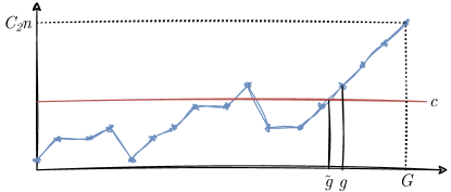
Figure S1: Cartoon of the objects in this proof. The points represent the discrete function $f:\mathbb{Z}_{G}\to\mathbb{R}$, and the interpolation $\tilde{f}$ simply connects these dots. The slope of any upwards sloping line is at most 2.

There are now two cases. If $\tilde{g}$ happens to be an integer, we are done. Otherwise, $\tilde{g}$ must sit on an upwards sloping line segment of $\tilde{f}$ (by assumption that $g\geq\tilde{g}\implies\tilde{f}(g)\geq\tilde{f}(\tilde{g})$). By virtue of the fact that adding one two-qubit gate increases entanglement entropy by at most 2, the slope of this line is at most 2, so defining $g=\lceil\tilde{g}\rceil$, we see that $0\leq f(g)-c=\tilde{f}(g)-\tilde{f}(\tilde{g})\leq 2$. This is to say, there is always a $g$ such that $\left|f(g)-c\right|\leq 2$.

To conclude, applying the Clifford unitary $U^{(g)}$ to the subset phase states realizes the ensemble that has (on average) the desired value of entanglement between $\operatorname{poly}\log n$ and $n$. We see the new ensemble $\mathcal{E}_{U^{(g)}}$ still exhibits pseudomagic with gap $\operatorname{poly}\log n$ vs. $n$, since the Clifford does not change its magic. ∎

We now prove the complementary statement: there also exist pseudoentangled ensembles where the low entanglement ensemble has maximal magic.

Theorem 15 (Pseudoentangled ensembles with high magic).

Let $\mathcal{E}$ be the pseudorandom ensemble of subset phase states with $\left|S\right|=\Theta(\operatorname{poly}\log n)$, which has been shown to exhibit pseudoentanglement in Ref. [31]. If the pseudorandom functions $f$ are 8-wise independent, there exists a product of efficient local unitaries $\tilde{U}=\bigotimes_{i=1}^{n}\tilde{U}_{i}$ such that the pseudorandom ensemble of states $\mathcal{E}_{\tilde{U}}$ has near maximal magic (as measured by $M_{\alpha}$ for $\alpha\in[0,2]$).

Proof.

Let $\operatorname{Haar}^{\otimes n}$ be the distribution over a product of $n$ independent single qubit Haar random unitaries.

(I) We will show that

$$Z\coloneqq\frac{1}{2^{n}}{\mathbb{E}}_{|\psi\rangle\sim\mathcal{E}}{\mathbb{E}}_{U\sim\operatorname{Haar}^{\otimes n}}\left[\sum_{P\in\mathbb{P}_{n}}\mathrm{tr}^{4}(P|\psi\rangle\!\langle\psi|)\right]=O(\exp(-n)).$$ (S71)

We first define $W\coloneqq{\mathbb{E}}_{U\sim\operatorname{Haar}_{1}}\left[(U^{\dagger})^{\otimes 4}(\sum_{P\in\mathbb{P}_{1}}P^{\otimes 4})U^{\otimes 4}\right]$, where $\operatorname{Haar}_{1}$ is the ensemble of single qubit Haar random unitaries. We can analytically calculate

$$W=\frac{8}{5}\Pi_{\textrm{sym}}+4\Pi^{\prime},$$ (S72)

where $\Pi^{\prime}$ is the projector onto the subspace spanned by $|0101\rangle-|0110\rangle-|1001\rangle+|1010\rangle$ and $|0011\rangle-|0110\rangle-|1001\rangle+|1100\rangle$. The details of $W$ are irrelevant: the important part is that, when written in the computational basis, all matrix elements of $W$ are bounded in magnitude by $\frac{8}{5}$. Therefore, all the matrix elements of $W^{\otimes n}$ are bounded in magnitude by $\left(\frac{8}{5}\right)^{n}$.

Using this, we rewrite

$$Z =\frac{1}{2^{n}}{\mathbb{E}}_{|\psi\rangle\sim\mathcal{E}}\mathrm{tr}(W^{\otimes n}|\psi\rangle\!\langle\psi|^{\otimes 4})$$ (S73)

$$=\frac{1}{2^{n}\left|S\right|^{4}}\sum_{\{x_{j}\},\{y_{j}\}}{\mathbb{E}}_{f}\left[(-1)^{\sum_{j}f(x_{j})+f(y_{j})}\right]\mathrm{tr}(W^{\otimes n}|x_{1},x_{2},x_{3},x_{4}\rangle\langle y_{1},y_{2},y_{3},y_{4}|),$$

where now $x_{j}\in S$ and $y_{j}\in S$. Our bound on the matrix elements of $W^{\otimes n}$ tells us $\left|\mathrm{tr}(W^{\otimes n}|x_{1},x_{2},x_{3},x_{4}\rangle\langle y_{1},y_{2},y_{3},y_{4}|)\right|\leq\left(\frac{8}{5}\right)^{n}$, so

$$Z\leq\left(\frac{4}{5}\right)^{n}\frac{1}{\left|S\right|^{4}}\sum_{\{x_{j}\},\{y_{j}\}}{\mathbb{E}}_{f}\left[(-1)^{\sum_{j}f(x_{j})+f(y_{j})}\right].$$ (S74)

The problem just reduces to bounding the number of nonzero elements in the sum. Since $f$ is $8$-wise independent, ${\mathbb{E}}_{f}\left[(-1)^{\sum_{j}f(x_{j})+f(y_{j})}\right]$ is only nonzero when the $x_{j},y_{j}$ can all be ‘paired up’. That is, any given bitstring must appear an even number of times in $\{x_{j}\}\cup\{y_{j}\}$. Therefore, the number of nonzero elements is at most $\left|S\right|^{4}\binom{8}{2,2,2,2}$, where $\binom{8}{2,2,2,2}=2520$ is a multinomial coefficient. The $\left|S\right|^{4}$ is because we can select 4 pairs from $\left|S\right|$, and there are $\binom{8}{2,2,2,2}$ ways of allocating these bitstrings amongst $x_{1},x_{2},x_{3},x_{4},y_{1},y_{2},y_{3},y_{4}$. So to conclude, $Z\leq 2520\left(\frac{4}{5}\right)^{n}$. For all $n\geq 70$ (which we assume for the rest of the proof), $Z\leq\left(\frac{9}{10}\right)^{n}$. To summarize, we arrive at

$${\mathbb{E}}_{U\sim\operatorname{Haar}^{\otimes n}}\left[{\mathbb{E}}_{\psi\sim\mathcal{E_{U}}}\left[\frac{1}{2^{n}}\sum_{P\in\mathbb{P}_{n}}\mathrm{tr}^{4}(P|\psi\rangle\!\langle\psi|)\right]\right]\leq\left(\frac{9}{10}\right)^{n},$$ (S75)

so there must be some $U^{*}=\bigotimes_{i=1}^{n}U_{i}$ such that ${\mathbb{E}}_{\psi\sim\mathcal{E_{U^{*}}}}\left[\frac{1}{2^{n}}\sum_{P\in\mathbb{P}_{n}}\mathrm{tr}^{4}(P|\psi\rangle\!\langle\psi|)\right]\leq\left(\frac{9}{10}\right)^{n}$. By Markov’s inequality, we see that

$${\mathsf{Pr}}_{|\psi\rangle\sim\mathcal{E_{U^{*}}}}\left[\frac{1}{2^{n}}\sum_{P\in\mathbb{P}_{n}}\mathrm{tr}^{4}(P|\psi\rangle\!\langle\psi|)\geq\left(\frac{19}{20}\right)^{n}\right]\leq\left(\frac{18}{19}\right)^{n},$$ (S76)

or

$${\mathsf{Pr}}_{|\psi\rangle\sim\mathcal{E_{U^{*}}}}\left[M_{2}({\psi})\leq\log_{2}(20/19)n\right]\leq\left(\frac{18}{19}\right)^{n},$$ (S77)

so the states of the pseudorandom ensemble $\mathcal{E_{U^{*}}}$ have magic $M_{2}=\Theta(n)$ with overwhelming probability.

(II) So far, we have established that for the ensemble $\mathcal{E}$ of pseudorandom subset phase states, there exists a unitary $U^{*}=\bigotimes_{i=1}^{n}U_{i}^{*}$ such that $\mathcal{E}_{U^{*}}$ has both high magic and unchanged entanglement. In order to finally show that $\mathcal{E}_{U^{*}}$ is also pseudorandom, however, via Lemma 10, we still have to show that $U^{*}$ can be constructed efficiently with a finite gate set. Luckily, the Solovay-Kitaev theorem guarantees that we can approximate even an inefficient $U^{*}$ in polynomial depth. Combining this with the continuity of pseudorandomness (SM III), entanglement, and magic, we can show that we do not need to exactly implement $U^{*}$. By the Solovay-Kitaev theorem, we can approximate each of the $U_{i}^{*}$ with a unitary $\tilde{U}_{i}$ such that

$$\left\|U_{i}^{*}-\tilde{U}_{i}\right\|\leq\frac{2^{-3n}}{n}$$ (S78)

and $\tilde{U}_{i}$ has $O(n\log n)$ depth. Then, defining $\tilde{U}\coloneqq\bigotimes_{i=1}^{n}\tilde{U}_{i}$, we see that

$$\left\|U^{*}-\tilde{U}\right\|\leq 2^{-3n}$$ (S79)

and $\tilde{U}$ is still a $O(n\log n)$ depth circuit.

Since $\mathcal{E}_{\tilde{U}}$ is pseudorandom (by the continuity of pseudorandomness) and $\tilde{U}$ is a product of local unitaries, it still exhibits (tunable) pseudoentanglement. To show that it exhibits near maximal magic, we can simply apply the continuity of magic (Corollary 8) to conclude that $M_{2}(\tilde{U}\psi\tilde{U}^{\dagger})$ differs from $M_{2}(U^{*}\psi(U^{*})^{\dagger})$ by an additive error of at most $O(\exp(-n))$. This is to say, $M_{2}(\tilde{U}{\psi}\tilde{U}^{\dagger})$ is still $\Theta(n)$ with overwhelming probability. This immediately allows us to conclude that $M_{\alpha}({\psi})=\Theta(n)$ for any $\alpha\in[0,2]$ with overwhelming probability over the choice of $|\psi\rangle\sim\mathcal{E}_{\tilde{U}}$. ∎

The following corollary is to the above theorem (Theorem 15) as Corollary 6 is to Theorem 14. We simply use the tools of the above proof to achieve the more flexible goal of tunable magic, while keeping entanglement the same.

Corollary 7 (Pseudoentangled ensembles with tunable magic).

For any $\alpha\in(0,2]$ and any $\Omega(\operatorname{poly}\log n)\leq g(n)\leq O(n)$, there exists a product of local unitaries $U$ such that $\mathbb{E}_{|\psi\rangle\sim\mathcal{E}_{U}}[M_{\alpha}(\psi)]=\Theta(g(n))$, where $\mathcal{E}$ is the ensemble of subset phase states.

Proof.

We first define some notation. First, observe that any product of single qubit rotations $U=\bigotimes_{i=1}^{n}U_{i}$ can be parameterized by a vector $\theta\in\mathbb{R}^{3n}$, as each single qubit rotation $U_{i}$ can be parameterized by three Euler angles. We will henceforth write $U(\theta)$ to denote the product of local unitaries parameterized by the angles $\theta$. Now, consider the ensemble $\mathcal{E}=\{\psi_{k}\}$ of subset phase states with $\left|S\right|=\Theta(\exp\operatorname{poly}\log n)$. On the other hand, Theorem 15 showed that there exists some $\theta^{*}\in\mathbb{R}^{3n}$ and some constant $C>0$ such that $M_{2}(U(\theta^{*})|\psi_{k}\rangle)\geq Cn$ with overwhelming probability over $k$. Now, let $\alpha\in(0,2]$ and define

$$f(t)\coloneqq\mathbb{E}_{|\psi_{k}\rangle\sim\mathcal{E}_{U(t\theta^{*})}}[M_{\alpha}(U(\psi_{k}))].$$ (S80)

Note that an immediate implication of Lemma 5 is that $f(0)\leq 2\operatorname{poly}\log n$, and by Theorem 15, $f(1)\geq Cn$ for some strictly positive constant $C$.

We now have the following line of argument. Let $\mathcal{H}$ be a $2^{n}$-dimensional Hilbert space with the metric given by the trace distance. $g_{k}:[0,1]\to\mathcal{H}$, defined by $t\mapsto U(t\theta^{*})|\psi_{k}\rangle$ is a continuous function. Also, as shown in Theorems 18 and 8, $M_{\alpha}:\mathcal{H}\to\mathbb{R}$ is also a continuous function. We define $f_{k}\coloneqq M_{\alpha}\circ g_{k}$ (which is again continuous, since we have just composed two continuous functions). Since $f(t)$ is then just the mean of $f_{k}(t)$, $f(t)$ is continuous as well. By the intermediate value theorem, for any $2\operatorname{poly}\log n\leq c\leq Cn$, there exists some $t\in[0,1]$ such that $f(t)=c$. Therefore, for any $2\operatorname{poly}\log n\leq c\leq Cn$, there is some transformation $U(t\theta^{*})$ such that $\mathbb{E}_{|\psi_{k}\rangle\sim U(t\theta^{*})}[M_{2}(\psi_{k})]=c$. Furthermore, this ensemble $\mathcal{E}_{U(t\theta^{*})}$ still exhibits pseudoentanglement (i.e., its entanglement is $O(\operatorname{poly}\log n)$ across all cuts). ∎

The above results show that for particular ensembles of states (namely, the subset phase states), we can efficiently maximize either the magic or entanglement, holding the other constant. Of course, we can maximize both simply by maximizing magic first and then the entanglement. However, both proofs only hold up to $\alpha=2$ Rényi entropies. We show below that we can simultaneously maximize both the magic and entanglement for any $\alpha$-Rényi entropy by using approximate $t$-designs [95, 96].

Theorem 16 (Simultaneous maximization of magic and entanglement by unitary designs).

For any ensemble $\mathcal{E}$ and any $\alpha\geq 1$, there exists a unitary $U^{*}$ with depth $O(n\alpha^{5+o(1)})$ such that $\mathcal{E}_{U^{*}}$ exhibits maximal entanglement and maximal magic, as measured by the $\alpha$-Rényi entanglement entropy and $\alpha$-stabilizer entropy.

Proof.

Random brickwork circuits are simply circuits where we apply a unitary $U_{1,2}\otimes U_{3,4}\otimes\ldots$ then $U_{2,3}\otimes U_{4,5}\otimes\ldots$, where each of the $U_{i,i+1}$ act on sites $i$ and $i+1$ and are drawn independently and Haar-randomly. We denote the distribution of random brickwork circuits with depth $O(n(2\alpha)^{5+o(1)})$ as $\nu_{\alpha}$. Ref. [97] showed that this distribution approximates up to the first $2\alpha$ moments of the Haar distribution with a small constant multiplicative error. That is, for any observable $O$, we have

$$\frac{{\mathbb{E}}_{U\sim\nu_{\alpha}}[\mathrm{tr}^{2\alpha}(U^{\dagger}OU|\psi\rangle\!\langle\psi|)]}{{\mathbb{E}}_{|\psi\rangle\sim\operatorname{Haar}}[\mathrm{tr}^{2\alpha}(O|\psi\rangle\!\langle\psi|)]}\in[1-\epsilon,1+\epsilon].$$ (S81)

Mirroring the proofs of Theorems 14 and 15, we can immediately conclude that the expectation of the logarithm of the $\alpha$ entanglement entropy and logarithm of the $\alpha$-stabilizer entropy both attain the Haar random value (up to an irrelevant constant multiplicative error). Therefore, there must be some $U^{*}$ in the support of $\nu_{\alpha}$ such that both the entanglement and magic characteristics of the resulting ensemble scale with the correpsonding Haar random values of $\alpha$-entanglement entropy and stabilizer $\alpha$-entropy. ∎

Supplemental Material V:  Quantum chaos: Proof of Theorem 4

Definition 5 (Quantum chaos).

Consider a unitary $U$. Its $2k$-point out-of-time-order correlators (OTOCs) [49, 50] are

$$C_{2k}(U)\coloneqq\frac{1}{d}\mathrm{tr}(\tilde{P}_{1}Q_{1}\tilde{P}_{2}Q_{2}\cdots\tilde{P}_{k}Q_{k}),$$ (S82)

where $P_{i}$ and $Q_{i}$ are non-identity Pauli operators for $i=1,\ldots,k$ and $\tilde{P}_{i}\coloneqq U^{{\dagger}}P_{i}U$. We say $U$ is chaotic if

$$C_{2k}(U)=\tilde{O}(C_{2k}(U_{\operatorname{Haar}})),$$ (S83)

where $\tilde{O}$ stands for an irrelevant polynomial overhead, and $C_{2k}(U_{\operatorname{Haar}})$ is the average of the $2k$-point OTOCs over Haar random unitaries.

Theorem 17 (Exponential separation from Haar values).

Let $\mathcal{E}$ be an ensemble of pseudomagic states. Let $|\psi\rangle\in\mathcal{E}$ and let $U$ such that $|\psi\rangle=U|0\rangle^{\otimes n}$. Then there exists $2k$-point OTOCs that are exponentially separated from the Haar value as

$$C_{2k}(U)=\Omega(\exp(n)C_{2k}(U_{\operatorname{Haar}}))$$ (S84)

and thus $U$ cannot be considered chaotic by Definition 5.

Proof.

The proof will be constructive. We simply construct a $2k$-point OTOC that exhibits exponential separation from the Haar average value. Let $U$ and $|\psi_{U}\rangle$ be unitary and state vector such that $|\psi_{U}\rangle=U|0\rangle^{\otimes n}$. Consider the $\alpha$-stabilizer entropy $M_{\alpha}(\psi_{U})$ with integer $\alpha>1$

$$M_{\alpha}({\psi_{U}})=\frac{1}{1-\alpha}\log\frac{1}{d}\sum_{P\in\mathbb{P}_{n}}\mathrm{tr}^{2\alpha}(\tilde{P}|0\rangle\!\langle 0|^{\otimes n})$$ (S85)

where $\tilde{P}\coloneqq U^{{\dagger}}PU$. Let us exploit the fact that $|0\rangle\!\langle 0|^{\otimes n}$ is pure to write $\mathrm{tr}^{2}(\tilde{P}|0\rangle\!\langle 0|^{\otimes n})=\mathrm{tr}(\tilde{P}|0\rangle\!\langle 0|^{\otimes n}\tilde{P}|0\rangle\!\langle 0|^{\otimes n})$ multiple times. Expanding $|0\rangle\!\langle 0|^{\otimes n}$ in terms of Pauli operators as $|0\rangle\!\langle 0|^{\otimes n}=d^{-1}\sum_{Z\in\mathbb{Z}_{n}}Z$ with $\mathbb{Z}_{n}$ the commuting subgroup of the Pauli group generated by single-qubit Pauli-$Z$s, we write

$$M_{\alpha}({\psi_{U}})=\frac{1}{1-\alpha}\log\frac{1}{d^{2\alpha+1}}\sum_{P,Z_{1},\ldots,Z_{2\alpha}}\mathrm{tr}(\tilde{P}Z_{1}\tilde{P}Z_{2}\cdots\tilde{P}Z_{2\alpha}).$$ (S86)

Now, let us denote by brackets $\langle\cdot\rangle_{\mathbb{P}_{n},\mathbb{Z}_{n}}$ the group average with respect to the whole Pauli group $\mathbb{P}_{n}$ and the subgroup $\mathbb{Z}_{n}$. Noting that $C_{4\alpha}(U,P,Z_{i})\coloneqq d^{-1}\mathrm{tr}(\tilde{P}Z_{1}\tilde{P}Z_{2}\cdots\tilde{P}Z_{2\alpha})$ is a $4\alpha$-point OTOC, let us define $C_{4\alpha}(U)\coloneqq\langle C_{4\alpha}(U,P,Z_{i})\rangle_{\mathbb{P}_{n},\mathbb{Z}_{n}}$ the averaged $4\alpha$ point OTOC. We can thus express the stabilizer entropy in terms of a single out of time ordered correlation function

$$M_{\alpha}({\psi_{U}})=\frac{1}{1-\alpha}\log d^{2}C_{4\alpha}(U).$$ (S87)

Now we are finally ready to show the main result. Let $|\psi_{PM}\rangle$ be a pseudomagic state satisfying $M_{\alpha}({\psi_{PM}})=o(n)$ (the subset phase states with $\left|S\right|=O(\exp\operatorname{poly}\log n)$ easily accomplish this). Let $|\psi_{\operatorname{Haar}}\rangle$ be a Haar random state. With overwhelming probability, one has $M_{\alpha}({\psi_{\operatorname{Haar}}})=\Omega(n/\alpha)$. Let us consider the difference

$$M_{\alpha}({\psi_{\operatorname{Haar}}})-M_{\alpha}({\psi_{PM}})=\Omega(n/\alpha).$$ (S88)

Denoting $U_{PM}$ the unitary that constructs $|\psi_{PM}\rangle=U_{PM}|0\rangle^{\otimes n}$ and $U_{\operatorname{Haar}}$ the equivalent for $|\psi_{\operatorname{Haar}}\rangle$, we readily get

$$C_{4\alpha}(U_{PM})=\Omega(\exp(n)C_{4\alpha}(U_{\operatorname{Haar}})).$$ (S89)

Defining $2k=4\alpha$ proves the statement. ∎

Supplemental Material VI:  Fannes inequality for $M_{1}$ and cryptography from pseudomagic: Proof of Theorem 5

Informally speaking, an EFI pair is a pair of efficient quantum algorithms whose output states are statistically far but computationally indistinguishable.

Definition 6 (EFI pairs [33]).

We call $\mu\coloneqq\left(\mu_{b,\lambda}\right)$ a pair of EFI states if it satisfies the following criteria:

• Efficient generation: There exists a uniform QPT quantum algorithm $A$ that on input $\left(1^{\lambda},b\right)$ for some integer $\lambda$ and $b\in\{0,1\}$, outputs the mixed state $\mu_{b,\lambda}$.

• Statistically distinguishable: ${\mathsf{TV}}\left(\mu_{0,\lambda},\mu_{1,\lambda}\right)\geq\Omega(\frac{1}{\operatorname{poly}\lambda})$.

• Computational indistinguishability: $\left(\mu_{0,\lambda}\right)_{\lambda}$ is computationally indistinguishable to $\left(\mu_{1,\lambda}\right)_{\lambda}$.

We will now show that pseudomagic ensembles imply EFI pairs. A critical ingredient in this proof will be a Fannes-type inequality which establishes for stabilizer entropy what the Fannes-Audenaert inequality establishes for entropy – namely its continuity in the space of states over the metric of trace distance. We now prove such an inequality for $M_{1}$. Since this proof is of independent interest, we devote a separate section to it before we prove the implication about EFI pairs.

VI.1 A Fannes Inequality for the Stabilizer Shannon Entropy

Recall from Eq. S3 that $M_{1}$ can be written

$$M_{1}(\psi)=-\sum_{P\in\mathbb{P}_{n}}\frac{\mathrm{tr}^{2}(P\psi)}{d}\log\mathrm{tr}^{2}(P\psi).$$ (S90)

Theorem 18 (Fannes-like inequality for $M_{1}$ (also to appear in Ref. [89])).

For any two states $|\psi\rangle$ and $|\phi\rangle$, it holds that

$$\left|M_{1}(\psi)-M_{1}(\phi)\right|\leq\begin{cases}\left\|\psi-\phi\right\|_{1}\log(d^{2}-1)+H_{\textrm{bin}}[\left\|\psi-\phi\right\|_{1}]&\text{for $\left\|\psi-\phi\right\|_{1}\leq 1/2$},\\ \left\|\psi-\phi\right\|_{1}\log(d^{2}-1)+1&\text{for $\left\|\psi-\phi\right\|_{1}>1/2$.}\\ \end{cases}$$ (S91)

Proof.

We make use of two main ingredients

• Consider a state vector $|\psi\rangle$ and its conjugate (in the computational basis) denoted as $|\psi^{*}\rangle$ and defined as $|\psi^{*}\rangle=\sum_{i}\langle i|\psi\rangle^{*}|i\rangle$. Define $|P\rangle:=I\otimes P|I\rangle$ where $|I\rangle=\frac{1}{\sqrt{d}}\sum_{i}|i\rangle\otimes|i\rangle$ the Bell state. Note that $\{|P\rangle\}$ is a basis for the Hilbert space $\mathcal{H}^{\otimes 2}$. The dephased state vector $|\psi\rangle\otimes|\psi^{*}\rangle$ (which we denote $|\psi\otimes\psi^{*}\rangle$ for short) in the basis $|P\rangle$ equals

  $$\mathcal{D}_{P}(\psi\otimes\psi^{*}):=\sum_{P}|P\rangle\!\langle P|\psi\otimes\psi^{*}|P\rangle\!\langle P|=\sum_{P}\frac{\mathrm{tr}^{2}(P\psi)}{d}|P\rangle\!\langle P|$$ (S92)

  indeed $\mel{P}{\psi\otimes\psi^{*}}{P}=\left|\langle\psi\otimes\psi^{*}|P\rangle\right|^{2}$. And

  $$\langle\psi\otimes\psi^{*}|P\rangle=\frac{1}{\sqrt{d}}\sum_{i}\langle\psi^{*}|i\rangle\mel{\psi}{P}{i}=\frac{1}{\sqrt{d}}\sum_{i}\mel{\psi}{P}{i}\langle i|\psi\rangle=\frac{\mel{\psi}{P}{\psi}}{\sqrt{d}}.$$ (S93)

• Moreover, let us show that $\left\|\psi\otimes\psi^{*}-\phi\otimes\phi^{*}\right\|_{1}=\left\|\psi^{\otimes 2}-\phi^{\otimes 2}\right\|_{1}$. To see this, note that

  $$\left\|\psi\otimes\psi^{*}-\phi\otimes\phi^{*}\right\|_{1}=2\sqrt{1-\mathrm{tr}(\psi\otimes\psi^{*}\phi\otimes\phi^{*})}=2\sqrt{1-\mathrm{tr}(\psi\phi)\mathrm{tr}(\psi^{*}\phi^{*})}$$ (S94)

  then consider $\mathrm{tr}(\psi^{*}\phi^{*})=\left|\langle\psi^{*}|\phi^{*}\rangle\right|^{2}$ and write it in the computational basis

  $$\langle\psi^{*}|\phi^{*}\rangle=\sum_{i}\langle\psi^{*}|i\rangle\langle i|\phi^{*}\rangle=\sum_{i}\langle\phi|i\rangle\langle i|\psi\rangle=\langle\phi|\psi\rangle$$ (S95)

  which implies $\mathrm{tr}(\psi^{*}\phi^{*})=\mathrm{tr}(\psi\phi)$. We used the definition of conjugate state, i.e. $|\psi^{*}\rangle=\sum_{i}(\langle i|\psi\rangle)^{*}|i\rangle\equiv\sum_{i}\langle\psi|i\rangle|i\rangle$. Returning to the $1$-norm distance, we have

  $$\left\|\psi\otimes\psi^{*}-\phi\otimes\phi^{*}\right\|_{1}=2\sqrt{1-\mathrm{tr}(\psi\phi)\mathrm{tr}(\psi^{*}\phi^{*})}=2\sqrt{1-\mathrm{tr}^{2}(\psi\phi)}=\left\|\psi^{\otimes 2}-\phi^{\otimes 2}\right\|_{1}.$$ (S96)

Consider now two pure states $\psi,\phi$ and the Shannon entropies $S(\Xi_{\psi}),S(\Xi_{\phi})$ of the (purely classical) probability distributions $\Xi_{\psi}(P),\Xi_{\phi}(P)$. The classical Fannes-Audenaert inequality for the Shannon entropy tells us

$$\left|S(\Xi_{\psi})-S(\Xi_{\phi})\right|\leq{\mathsf{TV}}(\Xi_{\psi},\Xi_{\phi})\log(d^{2}-1)+H_{\rm bin}[{\mathsf{TV}}(\Xi_{\psi},\Xi_{\phi})],$$ (S97)

where ${\mathsf{TV}}(\mathbf{p},\mathbf{q})\coloneqq\frac{1}{2}\sum_{i}\left|p_{i}-q_{i}\right|$ is the total variation distance between two probability distributions, and $H_{\rm bin}[x]$ is the binary entropy function $H_{\rm bin}[\epsilon]=-\epsilon\log\epsilon-(1-\epsilon)\log(1-\epsilon)$. Consider the state in Eq. S92 and notice that

$${\mathsf{TV}}(\Xi_{\psi},\Xi_{\phi})=\frac{1}{2}\sum_{P}\left|\Xi_{\psi}(P)-\Xi_{\phi}(P)\right|=\frac{1}{2}\left\|\mathcal{D}_{P}(\psi\otimes\psi^{*})-\mathcal{D}_{P}(\phi\otimes\phi^{*})\right\|_{1}$$ (S98)

simply represents the distance between the dephased states in the Bell basis. We can now combine Eq. S96 with the fact that the $1$-norm is non-increasing under any quantum channel (in this case, $\mathcal{D}_{P}$) to bound

$${\mathsf{TV}}(\Xi_{\psi},\Xi_{\phi})\leq\frac{1}{2}\left\|\psi^{\otimes 2}-\phi^{\otimes 2}\right\|_{1}\leq\left\|\psi-\phi\right\|_{1}.$$ (S99)

Assuming that $\left\|\psi-\phi\right\|_{1}\leq 1/2$ then ${\mathsf{TV}}(\Xi_{\psi},\Xi_{\phi})\leq 1/2$ and we have that $H_{\rm bin}$ is monotonic and we can write $H_{\rm bin}({\mathsf{TV}}(\Xi_{\psi},\Xi_{\phi}))\leq H_{\rm bin}(\left\|\psi-\phi\right\|_{1})$ and thus we can write

$$\left|M_{1}(\psi)-M_{1}(\phi)\right|\leq\left\|\psi-\phi\right\|_{1}\log(d^{2}-1)+H_{\rm bin}[\left\|\psi-\phi\right\|_{1}].$$ (S100)

Otherwise, if $\left\|\psi-\phi\right\|_{1}>1/2$, we can bound $H_{\rm bin}({\mathsf{TV}}(\Xi_{\psi},\Xi_{\phi}))\leq 1$

$$\left|M_{1}(|\psi\rangle)-M_{1}(|\phi\rangle)\right|\leq\left\|\psi-\phi\right\|_{1}\log(d^{2}-1)+1.$$ (S101)

∎

Following an identical technique to the above theorem, we can prove a much looser bound for higher $\alpha$.

Corollary 8 (Fannes-like inequality for $M_{\alpha>1}$).

For any $\alpha>1$ and any two state vectors $|\phi\rangle$ and $|\psi\rangle$,

$$\left|M_{\alpha}(\psi)-M_{\alpha}(\phi)\right|\leq\frac{d^{2}\alpha}{\alpha-1}\left\|\psi-\phi\right\|_{1}.$$ (S102)

Proof.

There are analogies to the Fannes-Audenaert inequality in Eq. S97 for classical Rényi entropies. In Eq. (20) of Ref. [98], it is shown that

$$\left|S_{\alpha}(\mathbf{p})-S_{\alpha}(\mathbf{q})\right|\leq\dim(\mathbf{p})\cdot\frac{\alpha}{\alpha-1}{\mathsf{TV}}(\mathbf{p},\mathbf{q}),$$ (S103)

for any $\alpha>1$ and any classical distributions $\mathbf{p},\mathbf{q}$ defined over $\dim(\mathbf{p})$ elements. In our case, this simply means

$$\left|S_{\alpha}(\Xi_{\psi})-S_{\alpha}(\Xi_{\phi})\right|\leq\frac{d^{2}\alpha}{\alpha-1}{\mathsf{TV}}(\Xi_{\psi},\Xi_{\phi})\leq\frac{d^{2}\alpha}{\alpha-1}\left\|\psi-\phi\right\|_{1},$$ (S104)

where the factor $d^{2}$ is because the classical distributions $\Xi_{\psi},\Xi_{\phi}$ are defined over all $d^{2}$ Pauli matrices. The second inequality follows from Eq. S99. ∎

VI.2 Proof of Theorem 5

Theorem 19 (EFI pairs from pseudo-magic ensembles (Theorem 5, repeated)).

Efficiently-generatable pseudo-magic ensembles with stabilizer 1-entropy that can be tuned between $\omega(\log n)$ and $n$ imply EFI pairs. Namely, we consider as the pair an algorithm that generates a random pseudo-magic state with magic of $\operatorname{poly}\log n$, and one that generates a random pseudo-magic state with magic of $n$.

Proof.

By a triangle inequality (since both ensembles are computationally indistinguishable from a Haar-random state), the outputs of these two algorithms are computationally indistinguishable from each other. It remains to show they are statistically distinguishable.

Let $|\psi\rangle$ be sampled from the first ensemble, which has magic $\Theta(\operatorname{poly}\log n)$ and $|\phi\rangle$ be sampled from the second ensemble, which has magic $\Theta(n)$. To show that the two ensembles are statistically distinguishable, it suffices to show that the two are far in trace distance, that is,

$$\left\|\psi-\phi\right\|_{1}\geq\Omega\left(\frac{1}{\operatorname{poly}n}\right).$$ (S105)

The continuity of the stabilizer Shannon entropy tells us that states which have very different magic must be far in trace distance. More specifically, Theorem 18 gives us

$$\left\|\psi-\phi\right\|_{1}\log(2^{2n}-1)\geq\Omega(n-\operatorname{poly}\log n),$$ (S106)

which is to say that

$$\left\|\psi-\phi\right\|_{1}\geq\Omega\left(1-\frac{\operatorname{poly}\log n}{n}\right)\geq\Omega\left(\frac{1}{\operatorname{poly}n}\right).$$ (S107)

∎

Supplemental Material VII:  Implications to magic-state distillation: Proof of Theorem 6

An immediate application of pseudorandom state ensembles with tunable stabilizer Rényi entropy is to derive new upper bounds on the problem of magic state distillation via stabilizer operations.

Theorem 20 (Bounds to magic state distillation).

Let $\mathcal{M}$ be a (sub-additive) magic monotone such that $\Omega(M_{\alpha})\leq\mathcal{M}\leq O(\mathcal{R})$ for some $\alpha=\Theta(1)$. Then any algorithm that uses stabilizer operations to synthesize a target quantum state $|B\rangle$ from copies of an arbitrary input state $\rho$ requires

$$\Omega\left(\frac{\mathcal{M}(|B\rangle\langle B|)}{\log^{1+c}(\mathcal{M}(\rho))}\right)$$ (S108)

copies of the input to succeed with non-negligible probability, where $c>0$.

Proof.

Assume towards contradiction that there is an algorithm that uses only a number

$$o\left(\frac{\mathcal{M}(|B\rangle)}{\log^{(1+c)}(\mathcal{M}(\rho))}\right)$$ (S109)

of copies of the (here possibly mixed) input $\rho$ to synthesize a single copy of the state $|B\rangle$, or equivalently, per copy of $\rho$, at least

$$\Omega\left(\frac{\log^{(1+c)}(\mathcal{M}(\rho))}{\mathcal{M}(|B\rangle\langle B|)}\right)$$ (S110)

copies of $|B\rangle$ may be synthesized.

As detailed in Ref. [27], a necessary condition to be able to synthesize a target quantum state $|B\rangle$ from an initial quantum state $\rho$ is that ${\cal M}(\rho)>{\cal M}(|B\rangle\langle B|)$ for any measure ${\cal M}$ of nonstabilizerness. This condition imposes that, per copy of $\rho$, at most

$$O\left(\frac{\mathcal{M}(\rho)}{\mathcal{M}(|B\rangle\langle B|)}\right)$$ (S111)

copies of $|B\rangle$ can be synthesized, where we have used the assumed sub-additivity of $\mathcal{M}$, i.e., $\mathcal{M}(\rho^{\otimes r})\leq r\mathcal{M}(\rho)$.

Recall our assumption that $\Omega(M_{\alpha})\leq\mathcal{M}\leq O(\mathcal{R})$, which implies that there exists positive constants $n_{0},s,s^{\prime}$ such that

$$sM_{\alpha}(\psi)\leq\mathcal{M}(\psi)\leq s^{\prime}\mathcal{R}(\psi)$$ (S112)

for all $n$-qubit states $\psi$ when $n>n_{0}$. For the rest of this proof, we will assume $n>n_{0}$. To prove our statement on the limitations of a distillation protocol that works on arbitrary input states $\rho$ (either pure or mixed), it is sufficient to focus on two special classes of input states, namely Haar random states and subset phase states. By combining Lemmas 4 and S112, we find that

$${\mathsf{Pr}}_{|\psi\rangle\sim\operatorname{Haar}}\left[\mathcal{M}(\psi)\leq\frac{s\beta n}{\alpha}\right]\leq 2^{-\frac{Cd^{1-2\beta}}{4(\alpha+1)^{2}}},$$ (S113)

for $C,\beta=O(1)$. Then, by our assumption in Eq. S110, the number of copies of $|B\rangle$ that could be synthesized with high probability per copy of $|\psi\rangle$ is

$$\Omega\left(\frac{\log^{(1+c)}(s\beta n/\alpha)}{\mathcal{M}(|B\rangle\langle B|)}\right).$$ (S114)

On the other hand, if $|\psi_{f,S}\rangle$ were a subset phase state with subset size $\left|S\right|=2^{\log^{1+c/2}(n)}$, combining Theorem 12 with Eq. S112 allows us to conclude

$$\mathcal{M}(\psi_{f,S})\leq s^{\prime}\log^{1+c/2}(n),$$ (S115)

then the upper bound in Eq. S111 translates into being able to synthesize no more than

$$O\left(\frac{\log^{(1+c/2)}(n)}{\mathcal{M}(|B\rangle\langle B|)}\right)$$ (S116)

copies of $|B\rangle$ per copy of $|\psi\rangle$. Then, a potential distinguisher handed $\operatorname{poly}(n)$ copies of an unknown $|\psi\rangle$ which is either one of these two types of states could simply run the black-box state synthesis protocol, count the number of copies of $|B\rangle$ synthesized with a SWAP test with a pre-existing copy of $|B\rangle$ – assumed to be a canonical state such as $|T\rangle$ – and thereby distinguish between these two states with high probability. Since the subset phase states are indistinguishable from Haar random states (given polynomially many copies), this is a contradiction. ∎

The above statement is deliberately agnostic concerning the magic monotone used, and is applicable for mixed resource states $\rho$ as well. Indeed, the powerful feature of constructing pseudomagic states is that, as pure states, no-go results can be proven using pseudomagic pure states and they remain valid for any state $\rho$ with appropriate extensions of magic monotones to mixed states. Moreover, it is well-known that while stabilizer entropies serve as effective magic measures (see SM I for details) for pure states, they fall short in quantifying the distillable magic for mixed states. This discrepancy arises because the set of states which have zero stabilizer entropy does not align with the corresponding set for other magic monotones, particularly those discussed in Table 1. Whereas the set of states for which stabilizer entropies is zero encompasses stabilizer-mixed states, as detailed in SM I, the set of zero magic monotones in Table 1 encompasses convex combinations of stabilizer states, known as the stabilizer polytope. However, the theorem mentioned above remains applicable to any magic monotone that is only bounded by some $\alpha=\Theta(1)$ stabilizer entropy and the robustness of magic for pure states. As we discuss below, whether this bound extends to mixed states as well is unimportant.

To be more specific, let us examine a significant example. Two prominent magic monotones used for distilling mixed states and for quantifying quantum speed-ups [99] are the max-relative entropy of magic denoted as $D_{\max}(\rho)$, and the mixed-state extent denoted as $\Xi(\rho)$. The former has been introduced in Table 1, while the latter is an extension of the stabilizer extent $\xi(\psi)$ defined for pure states. This extension, as commonly practiced in quantum resource theories, is achieved through a process known as convex-roof extension [99]

$$\Xi(\rho)\coloneqq\log\inf\left\{\sum_{j}p_{j}\xi(\psi_{j})\mid\rho=\sum_{j}p_{j}|\psi_{j}\rangle\langle\psi_{j}|\right\},$$ (S117)

applicable for mixed states, where the infimum is taken over pure state decompositions of $\rho$, as the convex hull or the convex roof of the stabilizer extent $\xi$, defined in Table 1. For pure states $\psi$, it holds that $\Xi(\psi)=D_{\max}(\psi)=\xi(\psi)$, i.e. both the max-relative entropy and the mixed-state extent reduce to the stabilizer extent $\xi(\psi)$ .

This enables us to further explore the consequences of Theorem 6. While for pure states $\psi$ it holds that

$$\Xi(\psi)=D_{\max}(\psi)=\xi(\psi)\leq\mathcal{R}(\psi),$$ (S118)

for mixed states $\rho$, the bounds are completely different [99]:

$$D_{\max}(\rho)\leq\Xi(\rho),\quad\log\left[2^{D_{\max}(\rho)+1}-1\right]\leq\mathcal{R}(\rho)$$ (S119)

whereas no known bound exists between $\Xi(\rho)$ and $\mathcal{R}(\rho)$. Similarly, no known bound exists between $\Xi$ and $M_{\alpha}$, as well as between $D_{\max}$ and $M_{\alpha}$ for mixed states. However, by virtue of Theorem 6, the following corollary holds.

Corollary 9 (Mixed state magic).

The mixed-state extent $\Xi$ and the max-relative entropy $D_{\max}(\rho)$ satisfy the conditions of Theorem 20 for $\alpha=2$ and thus they can be used as a measure to bound magic state distillation.

The above corollary reflects what was discussed earlier, i.e., the strength of our pseudomagic construction lies in the ability to leverage established bounds applicable to pure states, thereby drawing inferences for magic-state distillation applied to mixed states. Perhaps the most remarkable example of this is the observation that, despite stabilizer entropies having distinct null sets in the context of mixed states compared to other magic monotones, they can still be employed to draw conclusions regarding general magic-state distillation protocols.

It is also worth mentioning that in practical magic state distillation, one usually does not require perfect magic states $|B\rangle\langle B|$ to be distilled, but this is expected to be possible only approximately with high probability [99, 100, 2]. This is reminiscent of approximate asymptotic state transformations in entanglement theory. We here point out that statements of the above form can be made robust in the appropriate sense to capture such approximate state transformations. In the situation where $\rho^{\otimes k}$ is not exactly distilled to $|B\rangle\langle B|^{\otimes m}$, but where this happens probabilistically with some probability $p\in[0,1]$ in an approximate fashion, so that there exists an $\epsilon>0$ such that $\rho^{\otimes k}$ is transformed into $p\tau$ with the property that

$$\mathrm{tr}(\tau|B\rangle\!\langle B|^{\otimes m})\geq 1-\epsilon,$$ (S120)

then it necessarily holds that (see Ref. [99])

$$k\geq\frac{\log(p)+\log(1-\epsilon)+m\log F(|B\rangle\langle B|)^{-1}}{D_{\max}(\rho)},$$ (S121)

with $F(|B\rangle\langle B|)$ being the stabilizer fidelity of $|B\rangle\langle B|$. This can be used to state a robust version of the above theorem, in the sense of allowing for approximate state transformations.

Supplemental Material VIII:  Implications to property testing: Proof of Theorem 9

Definition 7 (Non-stabilizer tester).

An algorithm $\mathcal{A}_{\mathcal{M}}$ is a non-stabilizer tester if given $K$ copies of a state $|\psi\rangle$ and two threshold values $m,M\in[0,n]$ with $m<M$, obeys the following conditions.

• If $\mathcal{M}({\psi})\geq M$, then $\mathcal{A}_{\mathcal{M}}$ accepts $|\psi\rangle$ with probability $\geq\frac{2}{3}$.

• If $\mathcal{M}({\psi})<m$, then $\mathcal{A}_{\mathcal{M}}$ accepts $|\psi\rangle$ with probability $\leq\frac{1}{3}$.

The conditions above are referred to completness and soundness conditions, respectively.

In this section, we prove the following theorem.

Theorem 21 (Copies required for non-stabilizer testers).

Any tester for the stabilizer entropy $M_{\alpha}$ requires $K=\Omega(2^{\frac{m}{4+c}})$ (for $c>0$) copies for any $m<M<\frac{n}{4\alpha}$.

Proof.

First of all, by plugging $\beta=1/4$ into Lemma 4, we see that for a Haar random state vector $|\psi\rangle$,

$${\mathsf{Pr}}_{|\psi\rangle\sim\operatorname{Haar}}\left[M_{\alpha}({\psi})<\frac{n}{4\alpha}\right]<2^{-\Omega(2^{n/2})}.$$ (S122)

Consequently, one has that for any $M<n/(4\alpha)$ one can write ${\mathsf{Pr}}_{|\psi\rangle\sim\operatorname{Haar}}\left[M_{\alpha}({\psi})<M\right]<2^{-\Omega(2^{n/2})}$. Let us now define the ensembles

$$\mathcal{E}_{M_{\alpha}\geq M} \coloneqq\{|\psi\rangle\mid M_{\alpha}({\psi})\geq M\},$$ (S123)

$$\mathcal{E}_{M_{\alpha}<M} \coloneqq\{|\psi\rangle\mid M_{\alpha}({\psi})<M\}$$

of states with $\alpha$-stabilizer entropy at least $M$ and at most $M$. We use the notation $\Phi_{\mathcal{E}}^{(K)}$ to denote the ensemble average

$$\Phi_{\mathcal{E}}^{(K)}={\mathbb{E}}_{|\psi\rangle\sim\mathcal{E}}\left[|\psi\rangle\!\langle\psi|^{\otimes K}\right],$$ (S124)

where $\sim$ denotes the uniform distribution over $\mathcal{E}$. We show that the ensemble $\mathcal{E}_{M_{\alpha}>M}$ is exponentially close to the ensemble of Haar random state, i.e.,

$$\left\|\Phi_{\mathcal{E}_{M_{\alpha}\geq M}}^{(K)}-\Phi_{\operatorname{Haar}}^{(K)}\right\|_{1}=O(2^{-\Omega(2^{n/2})}).$$ (S125)

First of all note that denoting $\pi_{M}\coloneqq{\mathsf{Pr}}_{|\psi\rangle\sim\operatorname{Haar}}\left[M_{\alpha}({\psi})<M\right]$, we have $\pi_{M}\leq 2^{-\Omega(2^{n/2})}$. Notice that we can express $\Phi_{\operatorname{Haar}}^{(K)}$ for every $K$ as

$$\Phi_{\operatorname{Haar}}^{(K)}=\pi_{M}\Phi_{\mathcal{E}_{M_{\alpha}<M}}^{(K)}+(1-\pi_{M})\Phi_{\mathcal{E}_{M_{\alpha}\geq M}}^{(K)},$$ (S126)

thus the following chain of equalities and inequality holds,

$$\left\|\Phi_{\mathcal{E}_{M_{\alpha}\geq M}}^{(K)}-\Phi_{\operatorname{Haar}}^{(K)}\right\|_{1} =\left\|\Phi_{\mathcal{E}_{M_{\alpha}\geq M}}^{(K)}-\pi_{M}\Phi_{\mathcal{E}_{M_{\alpha}<M}}^{(K)}-(1-\pi_{M})\Phi_{\mathcal{E}_{M_{\alpha}\geq M}}^{(K)}\right\|_{1}$$ (S127)

$$=\left\|-\pi_{M}\Phi_{\mathcal{E}_{M_{\alpha}<M}}^{(K)}+\pi_{M}\Phi_{\mathcal{E}_{M_{\alpha}\geq M}}^{(K)}\right\|_{1}$$

$$=\pi_{M}\left\|\Phi_{\mathcal{E}_{M_{\alpha}<M}}^{(K)}-\Phi_{\mathcal{E}_{M_{\alpha}\geq M}}^{(K)}\right\|_{1}\leq\pi_{M}.$$

Now, consider the set $\mathcal{E}_{f,S}$ of subset phase states, i.e.,

$$|\psi_{f,S}\rangle=\frac{1}{\sqrt{\left|S\right|}}\sum_{x\in S}(-1)^{f(x)}|x\rangle,$$ (S128)

where both the Boolean function $x\mapsto f(x)$ and the subset $S$ have been chosen at random. Then, from Theorem $2.1$ of Ref. [31] we have that for every $K<\left|S\right|<d$

$$\left\|\Phi_{\mathcal{E}_{f,S}}^{(K)}-\Phi_{\operatorname{Haar}}^{(K)}\right\|_{1}=O\left(\frac{K^{2}}{\left|S\right|}\right),$$ (S129)

and consequently one has

$$\left\|\Phi_{\mathcal{E}_{M_{\alpha}\geq M}}^{(K)}-\Phi_{\mathcal{E}_{f,S}}^{(K)}\right\|_{1}\leq\left\|\Phi_{\mathcal{E}_{f,S}}^{(K)}-\Phi_{\operatorname{Haar}}^{(K)}\right\|_{1}+\left\|\Phi_{\mathcal{E}_{M_{\alpha}\geq M}}^{(K)}-\Phi_{\operatorname{Haar}}^{(K)}\right\|_{1}=O\left(\frac{K^{2}}{\left|S\right|}\right).$$ (S130)

The above equation implies that the ensemble of phase states and the ensemble of states with stabilizer entropy $M_{\alpha}({\psi})\geq M$ (for $M\leq n/(4\alpha)$) cannot be distinguished by a non-stabilizer tester unless $K=\Omega(\sqrt{\left|S\right|})$. Indeed, following the arguments of Ref. [76], by applying the Helstrom bound [101], we know for any state discrimination protocol between two ensembles $\mathcal{E},\mathcal{E}^{\prime}$ the discrimination probability given $K$ copies, is upper bounded by $\frac{1}{2}+\left\|\Phi_{\mathcal{E}}^{(K)}-\Phi_{\mathcal{E}^{\prime}}^{(K)}\right\|_{1}$. Therefore, for a non-stabilizer tester $\mathcal{A}_{\mathcal{M}}$, to have a acceptance probability $\geq 2/3$ one should have

$$\left\|\Phi_{\mathcal{E}_{M_{\alpha}\geq M}}^{(K)}-\Phi_{\mathcal{E}_{f,S}}^{(K)}\right\|_{1}\geq\frac{1}{6}.$$ (S131)

To conclude the proof, observe that $|\psi\rangle\in\mathcal{E}_{f,S}\implies M_{\alpha}({\psi})\leq\log\left|S\right|$, so $K=\Omega\left(2^{\frac{m}{4+c}}\right)$ for $c>0$. Indeed, if we assume that $K=O\left(2^{\frac{m}{4+c}}\right)$ copies were sufficient, one could take a random subset phase state $|\psi\rangle\in\mathcal{E}_{f,S}$ with $\left|S\right|=2^{m/2}$ having $M_{\alpha}({\psi})\leq m$ for $c>0$ and could distinguish between $|\psi\rangle\in\mathcal{E}_{f,S}$ and $|\psi\rangle\in\mathcal{E}_{M_{\alpha}\geq M}$ with $K=O\left(2^{\frac{m}{4+c}}\right)$. However, from Eq. S130 one would need

$$K=\Omega\left(\sqrt{\left|S\right|}\right)=\Omega(2^{m/4})$$ (S132)

copies to achieve this discrimination, so we have arrived at a contradiction. ∎

Corollary 10 (Property testers for magic monotones).

Given any magic monotone $\mathcal{M}$ such that $\mathcal{M}\geq sM_{\alpha}$ for some $\alpha,s$, a property tester for $\mathcal{M}$ requires $K=\Omega(2^{\frac{m/s}{4+c}})$.

Proof.

Consider a magic monotone $\mathcal{M}$ such that $\mathcal{M}\geq sM_{\alpha}$. Assuming the contrapositive, i.e., that one can use $O(2^{\frac{m/s}{4+c}})$ to distinguish whether a state vector $|\psi\rangle$ has $\mathcal{M}({\psi})\leq m$. However, if one could do so, one also would have distinguished $M_{\alpha}({\psi})\leq m/s$ using $O(2^{\frac{m/s}{4+c}})$ copies and this is a contradiction to Theorem 9. ∎

References

- Bravyi and Kitaev [2005a] S. Bravyi and A. Kitaev, Phys. Rev. A 71, 022316 (2005a).
- Howard and Campbell [2017a] M. Howard and E. Campbell, Phys. Rev. Lett. 118, 090501 (2017a).
- Bartlett [2014] S. D. Bartlett, Nature 510, 345 (2014).
- Gottesman [1997] D. Gottesman, Stabilizer codes and quantum error correction (1997), quant-ph/9705052 .
- Aaronson and Gottesman [2004a] S. Aaronson and D. Gottesman, Phys. Rev. A 70, 052328 (2004a).
- Bravyi and Gosset [2016] S. Bravyi and D. Gosset, Phys. Rev. Lett. 116, 250501 (2016).
- Bravyi et al. [2016] S. Bravyi, G. Smith, and J. A. Smolin, Phys. Rev. X 6, 021043 (2016).
- Bravyi et al. [2019] S. Bravyi, D. Browne, P. Calpin, E. Campbell, D. Gosset, and M. Howard, Quantum 3, 181 (2019).
- Seddon et al. [2021a] J. R. Seddon, B. Regula, H. Pashayan, Y. Ouyang, and E. T. Campbell, PRX Quantum 2, 010345 (2021a).
- Mari and Eisert [2012] A. Mari and J. Eisert, Phys. Rev. Lett. 109, 230503 (2012).
- Veitch et al. [2014] V. Veitch, S. A. H. Mousavian, D. Gottesman, and J. Emerson, New J. Phys. 16, 013009 (2014).
- Veitch et al. [2012] V. Veitch, C. Ferrie, D. Gross, and J. Emerson, New J. Phys. 14, 113011 (2012).
- Howard and Campbell [2017b] M. Howard and E. T. Campbell, Phys. Rev. Lett. 118, 090501 (2017b).
- O'Gorman and Campbell [2017] J. O'Gorman and E. T. Campbell, Phys. Rev. A 95, 032338 (2017).
- Bravyi and Haah [2012a] S. Bravyi and J. Haah, Phys. Rev. A 86, 052329 (2012a).
- Campbell and Howard [2017a] E. T. Campbell and M. Howard, Phys. Rev. A 95, 022316 (2017a).
- Campbell and Howard [2017b] E. T. Campbell and M. Howard, Phys. Rev. Lett. 118, 060501 (2017b).
- Campbell [2011] E. T. Campbell, Phys. Rev. A 83, 032317 (2011).
- Dawkins and Howard [2015] H. Dawkins and M. Howard, Phys. Rev. Lett. 115, 030501 (2015).
- Campbell and Browne [2010a] E. T. Campbell and D. E. Browne, Phys. Rev. Lett. 104, 030503 (2010a).
- Anwar et al. [2012] H. Anwar, E. T. Campbell, and D. E. Browne, New J. Phys. 14, 063006 (2012).
- Krishna and Tillich [2019] A. Krishna and J.-P. Tillich, Phys. Rev. Lett. 123, 070507 (2019).
- Kitaev [2003] A. Y. Kitaev, Ann. Phys. 303, 2 (2003).
- Campbell and Browne [2010b] E. T. Campbell and D. E. Browne, Phys. Rev. Lett. 104, 030503 (2010b).
- Campbell et al. [2017] E. T. Campbell, B. M. Terhal, and C. Vuillot, Nature 549, 172–179 (2017).
- Xu et al. [2023] Q. Xu, J. P. B. Ataides, C. A. Pattison, N. Raveendran, D. Bluvstein, J. Wurtz, B. Vasic, M. D. Lukin, L. Jiang, and H. Zhou, Constant-overhead fault-tolerant quantum computation with reconfigurable atom arrays (2023), arXiv:2308.08648 .
- Leone et al. [2022] L. Leone, S. F. E. Oliviero, and A. Hamma, Phys. Rev. Lett. 128, 050402 (2022).
- Leone et al. [2023a] L. Leone, S. F. E. Oliviero, and A. Hamma, Phys. Rev. A 107, 022429 (2023a).
- Goto et al. [2022a] K. Goto, T. Nosaka, and M. Nozaki, Phys. Rev. D 106, 126009 (2022a).
- Garcia et al. [2023] R. J. Garcia, K. Bu, and A. Jaffe, Proc. Natl. Ac. Sc. 120, e2217031120 (2023).
- Aaronson et al. [2023] S. Aaronson, A. Bouland, B. Fefferman, S. Ghosh, U. Vazirani, C. Zhang, and Z. Zhou, Quantum pseudoentanglement (2023), arXiv:2211.00747 .
- Liu and Winter [2022a] Z.-W. Liu and A. Winter, PRX Quantum 3, 020333 (2022a).
- Brakerski et al. [2022] Z. Brakerski, R. Canetti, and L. Qian, On the computational hardness needed for quantum cryptography (2022), arXiv:2209.04101 .
- Gottesman [1998] D. Gottesman, The Heisenberg representation of quantum computers (1998), quant-ph/9807006 .
- Tirrito et al. [2023] E. Tirrito, P. S. Tarabunga, G. Lami, T. Chanda, L. Leone, S. F. E. Oliviero, M. Dalmonte, M. Collura, and A. Hamma, Quantifying non-stabilizerness through entanglement spectrum flatness (2023), 2304.01175 .
- Haug and Piroli [2023a] T. Haug and L. Piroli, Stabilizer entropies and nonstabilizerness monotones (2023a), arXiv:2303.10152 .
- Haug et al. [2023a] T. Haug, S. Lee, and M. S. Kim, Efficient stabilizer entropies for quantum computers (2023a), 2305.19152 .
- Haug and Kim [2023] T. Haug and M. Kim, PRX Quantum 4, 010301 (2023).
- Bu et al. [2023a] K. Bu, W. Gu, and A. Jaffe, PNAS 120, e2304589120 (2023a).
- Bu et al. [2023b] K. Bu, W. Gu, and A. Jaffe, Stabilizer testing and magic entropy (2023b), arXiv:2306.09292 .
- Chamon et al. [2022] C. Chamon, E. R. Mucciolo, and A. E. Ruckenstein, Ann. Phys. 446, 169086 (2022).
- Turkeshi et al. [2023] X. Turkeshi, M. Schirò, and P. Sierant, Measuring magic via multifractal flatness (2023), arXiv:2305.11797 .
- Saxena and Gour [2022] G. Saxena and G. Gour, Phys. Rev. A 106, 042422 (2022).
- Koukoulekidis and Jennings [pril] N. Koukoulekidis and D. Jennings, npj Quant. Inf. 8, 1 (2022/april).
- Note [1] Note that the ensemble of Haar random states is only one of many ensembles that have high magic. In general, pseudomagic states need not be indistinguishable from Haar random states; however, the definition of pseudomagic states requires that there is at least one ensemble of high magic states that they are indistinguishable from.
- Note [2] We will make frequent use of asymptotic, or Bachmann–Landau, notation. To remind the reader, , , and finally such that .
- Ji et al. [2018] Z. Ji, Y.-K. Liu, and F. Song, in Advances in Cryptology – CRYPTO 2018, edited by H. Shacham and A. Boldyreva (Springer International Publishing, Cham, 2018) pp. 126–152.
- Beverland et al. [2020] M. Beverland, E. Campbell, M. Howard, and V. Kliuchnikov, Quant. Sc. Tech. 5, 035009 (2020).
- Roberts and Yoshida [2017] D. A. Roberts and B. Yoshida, JHEP 2017 (4), 121.
- Hosur et al. [2016] P. Hosur, X.-L. Qi, D. A. Roberts, and B. Yoshida, JHEP 2016 (2), 4.
- Leone et al. [2021a] L. Leone, S. F. E. Oliviero, and A. Hamma, Entropy 23, 1073 (2021a).
- Oliviero et al. [2021a] S. F. E. Oliviero, L. Leone, F. Caravelli, and A. Hamma, SciPost Physics 10, 76 (2021a).
- Goto et al. [2022b] K. Goto, T. Nosaka, and M. Nozaki, Phys. Rev. D 106, 126009 (2022b).
- Leone et al. [2021b] L. Leone, S. F. E. Oliviero, Y. Zhou, and A. Hamma, Quantum 5, 453 (2021b).
- Oliviero et al. [2021b] S. F. E. Oliviero, L. Leone, and A. Hamma, Physics Letters A 418, 127721 (2021b).
- Kretschmer [2021] W. Kretschmer (Schloss Dagstuhl - Leibniz-Zentrum für Informatik, 2021).
- Morimae and Yamakawa [2022] T. Morimae and T. Yamakawa, in Advances in Cryptology – CRYPTO 2022 (Springer Nature Switzerland, 2022) pp. 269–295.
- Lin et al. [2014] D. Lin, Y. Quan, J. Weng, and J. Yan, Quantum bit commitment with application in quantum zero-knowledge proof, Cryptology ePrint Archive, Paper 2014/791 (2014).
- Yan [2020] J. Yan, General properties of quantum bit commitments, Cryptology ePrint Archive, Paper 2020/1488 (2020).
- Bartusek et al. [2021] J. Bartusek, A. Coladangelo, D. Khurana, and F. Ma, in Advances in Cryptology – CRYPTO 2021, edited by T. Malkin and C. Peikert (Springer International Publishing, Cham, 2021) pp. 467–496.
- Grilo et al. [2021] A. B. Grilo, H. Lin, F. Song, and V. Vaikuntanathan, in Advances in Cryptology – EUROCRYPT 2021, edited by A. Canteaut and F.-X. Standaert (Springer International Publishing, Cham, 2021) pp. 531–561.
- Ananth et al. [2022] P. Ananth, L. Qian, and H. Yuen, in Advances in Cryptology – CRYPTO 2022, edited by Y. Dodis and T. Shrimpton (Springer Nature Switzerland, Cham, 2022) pp. 208–236.
- Ananth et al. [2021] P. Ananth, K.-M. Chung, and R. L. L. Placa, in Advances in Cryptology – CRYPTO 2021, edited by T. Malkin and C. Peikert (Springer International Publishing, Cham, 2021) pp. 346–374.
- Bravyi and Kitaev [2005b] S. Bravyi and A. Kitaev, Phys. Rev. A 71, 022316 (2005b).
- Knill [2005] E. Knill, Nature 434, 39 (2005).
- Bravyi and Haah [2012b] S. Bravyi and J. Haah, Phys. Rev. A 86, 052329 (2012b).
- Harrow [2005] A. Harrow, Applications of coherent classical communication and the Schur transform to quantum information theory, Ph.D. thesis, Massachusetts Institute of Technology (2005).
- Hayashi and Matsumoto [2002] M. Hayashi and K. Matsumoto, Universal distortion-free entanglement concentration (2002), quant-ph/0209030 .
- Bennett et al. [1996] C. H. Bennett, G. Brassard, S. Popescu, B. Schumacher, J. A. Smolin, and W. K. Wootters, Phys. Rev. Lett. 76, 722–725 (1996).
- Bao et al. [2022] N. Bao, C. Cao, and V. P. Su, Phys. Rev. A 105, 10.1103/physreva.105.022602 (2022).
- Arute et al. [2019] F. Arute, K. Arya, R. Babbush, D. Bacon, J. C. Bardin, R. Barends, R. Biswas, S. Boixo, F. G. S. L. Brandao, D. A. Buell, B. Burkett, Y. Chen, Z. Chen, B. Chiaro, R. Collins, W. Courtney, A. Dunsworth, E. Farhi, B. Foxen, A. Fowler, C. Gidney, M. Giustina, R. Graff, K. Guerin, S. Habegger, M. P. Harrigan, M. J. Hartmann, A. Ho, M. Hoffmann, T. Huang, T. S. Humble, S. V. Isakov, E. Jeffrey, Z. Jiang, D. Kafri, K. Kechedzhi, J. Kelly, P. V. Klimov, S. Knysh, A. Korotkov, F. Kostritsa, D. Landhuis, M. Lindmark, E. Lucero, D. Lyakh, S. Mandrà, J. R. McClean, M. McEwen, A. Megrant, X. Mi, K. Michielsen, M. Mohseni, J. Mutus, O. Naaman, M. Neeley, C. Neill, M. Y. Niu, E. Ostby, A. Petukhov, J. C. Platt, C. Quintana, E. G. Rieffel, P. Roushan, N. C. Rubin, D. Sank, K. J. Satzinger, V. Smelyanskiy, K. J. Sung, M. D. Trevithick, A. Vainsencher, B. Villalonga, T. White, Z. J. Yao, P. Yeh, A. Zalcman, H. Neven, and J. M. Martinis, Nature 574, 505 (2019).
- Bouland et al. [2018] A. Bouland, B. Fefferman, C. Nirkhe, and U. Vazirani, Nature Physics 15, 159 (2018).
- Cubitt and Montanaro [2016] T. Cubitt and A. Montanaro, Complexity classification of local hamiltonian problems (2016), arXiv:1311.3161 [quant-ph] .
- Liu and Winter [2022b] Z.-W. Liu and A. Winter, PRX Quantum 3, 020333 (2022b).
- Levine et al. [2019] H. Levine, A. Keesling, G. Semeghini, A. Omran, T. T. Wang, S. Ebadi, H. Bernien, M. Greiner, V. Vuletić , H. Pichler, and M. D. Lukin, Phys. Rev. Lett. 123, 170503 (2019).
- Haug et al. [2023b] T. Haug, K. Bharti, and D. E. Koh, Pseudorandom unitaries are neither real nor sparse nor noise-robust (2023b), arXiv:2306.11677 .
- Oliviero et al. [2022a] S. F. E. Oliviero, L. Leone, and A. Hamma, Phys. Rev. A 106, 042426 (2022a).
- Lami and Collura [2023] G. Lami and M. Collura, Quantum magic via perfect Pauli sampling of matrix product states (2023), arXiv:2303.05536 .
- Haug and Piroli [2023b] T. Haug and L. Piroli, Phys. Rev. B 107, 035148 (2023b).
- Chen et al. [2022] L. Chen, R. J. Garcia, K. Bu, and A. Jaffe, Magic of random matrix product states (2022), arXiv:2211.10350 .
- Odavić et al. [2022] J. Odavić, T. Haug, G. Torre, A. Hamma, F. Franchini, and S. M. Giampaolo, Complexity of frustration: A new source of non-local non-stabilizerness (2022), arXiv:2209.10541 .
- Rattacaso et al. [2023] D. Rattacaso, L. Leone, S. F. E. Oliviero, and A. Hamma, Stabilizer entropy dynamics after a quantum quench (2023), arXiv:2304.13768 .
- Tarabunga et al. [2023] P. S. Tarabunga, E. Tirrito, T. Chanda, and M. Dalmonte, Many-body magic via Pauli-Markov chains – from criticality to gauge theories (2023), arXiv:2305.18541 .
- Chen et al. [2023] J. Chen, Y. Yan, and Y. Zhou, Magic of quantum hypergraph states (2023), arXiv:2308.01886 .
- Halpern et al. [2022] N. Y. Halpern, N. B. T. Kothakonda, J. Haferkamp, A. Munson, J. Eisert, and P. Faist, Phys. Rev. A 106, 10.1103/physreva.106.062417 (2022).
- Note [3] More precisely, the robustness of magic [13] is upper bounded by as proven in Ref. [32].
- Heinrich and Gross [2019] M. Heinrich and D. Gross, Quantum 3, 132 (2019).
- Oliviero et al. [2022b] S. F. E. Oliviero, L. Leone, A. Hamma, and S. Lloyd, npj Quant. Inf. 8, 1 (2022b).
- Leone [2023] L. Leone, Clifford Group and beyond: Theory and Applications in Quantum Information, Ph.D. thesis, University of Massachusetts Boston – in preparation (2023).
- Jiang and Wang [2021] J. Jiang and X. Wang, Lower bound the T-count via unitary stabilizer nullity (2021), 2103.09999 .
- Leone et al. [2023b] L. Leone, S. F. E. Oliviero, and A. Hamma, Learning t-doped stabilizer states (2023b), arXiv:2305.15398 .
- Grewal et al. [2023] S. Grewal, V. Iyer, W. Kretschmer, and D. Liang, Improved stabilizer estimation via bell difference sampling (2023), arXiv:2304.13915 .
- Aaronson and Gottesman [2004b] S. Aaronson and D. Gottesman, Phys. Rev. A 70, 052328 (2004b).
- Liu et al. [2018] Z.-W. Liu, S. Lloyd, E. Zhu, and H. Zhu, JHEP 2018 (7).
- Gross et al. [2007] D. Gross, K. Audenaert, and J. Eisert, J. Math. Phys. 48, 052104 (2007).
- Haferkamp et al. [2023] J. Haferkamp, F. Montealegre-Mora, M. Heinrich, J. Eisert, D. Gross, and I. Roth, Commun. Math. Phys. 397, 995 (2023).
- Haferkamp [2022] J. Haferkamp, Quantum 6, 795 (2022).
- Hanson and Datta [2019] E. P. Hanson and N. Datta, Universal proofs of entropic continuity bounds via majorization flow (2019), arXiv:1909.06981 .
- Seddon et al. [2021b] J. R. Seddon, B. Regula, H. Pashayan, Y. Ouyang, and E. T. Campbell, PRX Quantum 2, 010345 (2021b).
- Fang and Liu [2020] K. Fang and Z.-W. Liu, Phys. Rev. Lett. 125, 060405 (2020).
- Bae and Kwek [2015] J. Bae and L.-C. Kwek, J. Phys. A 48, 083001 (2015).