MASA-TCN: Multi-anchor Space-aware Temporal Convolutional Neural Networks for Continuous and Discrete EEG Emotion Recognition

Abstract

Emotion recognition using electroencephalogram (EEG) mainly has two scenarios: classification of the discrete labels and regression of the continuously tagged labels. Although many algorithms were proposed for classification tasks, there are only a few methods for regression tasks. For emotion regression, the label is continuous in time. A natural method is to learn the temporal dynamic patterns. In previous studies, long short-term memory (LSTM) and temporal convolutional neural networks (TCN) were utilized to learn the temporal contextual information from feature vectors of EEG. However, the spatial patterns of EEG were not effectively extracted. To enable the spatial learning ability of TCN towards better regression and classification performances, we propose a novel unified model, named MASA-TCN, for EEG emotion regression and classification tasks. The space-aware temporal layer enables TCN to additionally learn from spatial relations among EEG electrodes. Besides, a novel multi-anchor block with attentive fusion is proposed to learn dynamic temporal dependencies. Experiments on two publicly available datasets show MASA-TCN achieves higher results than the state-of-the-art methods for both EEG emotion regression and classification tasks. The code is available at https://github.com/yi-ding-cs/MASA-TCN.

1 Introduction

Emotion recognition aims at enabling machines to perceive human emotions using machine learning technologies. It is also known as emotional artificial intelligence [1, 2]. Emotion is one of the essential elements in human’s daily life, playing an impotent role in decision-making, human interaction, and intelligence [3]. It can be measured by categorical and dimensional models. A common emotion model is the valence-arousal-dominance (VAD) model, which measures emotion in valence, arousal, and dominance dimensions. Valence dimension reflects emotion from negative to positive; arousal indicates the emotional state from passive to active; dominance represents how strong the emotion is [1]. Emotion can be reflected in several types of affective signals, such as physiological signals, speech and facial expressions [4]. Electroencephalogram (EEG) is one of the wildly utilized brain imaging technologies in brain-computer interface due to its cost-efficiency, non-invasive usage, and easy operation. Compared with other affective modalities that can be disguised by the subject, EEG can reflect brain’s intrinsic emotional neural activities more directly.

We introduce and disambiguate discrete emotional state classification (DEC) and continuous emotion regression (CER), two representative tasks in EEG emotion recognition. Generally, four aspects are covered, i.e., the data acquisition, data annotation, representation learning, and result evaluation. For the data acquisition, the same protocol can be shared by the two tasks. Usually, every subject is required to watch a certain number of short film clips, during which their facial expression, EEG signals, and other emotional cues are recorded [5, 6, 7]. The recordings could last from several seconds to minutes, depending on the stimulus length. The differences of DEC and CER exist in the rest three aspects. For the annotation, DEC would assign only one discrete label to a trial [8]. But CER would assign one unique label to every one or several data points, so that a trial is labeled by a trace of changing values [9]. For the representation learning, while the long-term temporal dynamics might be downplayed by the DEC models, they are the cornerstones for a successful sequence prediction, which is the goal of the CER models. As for the evaluation, DEC follows a standard classification scenario, where the accuracy and F1 score are usually employed [8]. CER, on the other hands, requires a consistency measure, which usually refers to RMSE, PCC, and CCC [9]. Both of DEC and CER are challenging due to the low signal-to-noise ratio (SNR) and unstable statistical characteristics of EEG signals, especially under generalized experiment settings in where the test data is never seen by the classifier during training [8].

Those challenges catch many researchers’ interest in recent years [1], especially for DEC tasks. For DEC tasks, traditionally, different types of features are extracted from the pre-processed EEG signals, such as power spectral density (PSD), differential entropy (DE), differential asymmetry (DASM), and rational asymmetry (RASM) [10]. Then the shallow learning methods were applied, such as support vector machine (SVM) and k-nearest neighborhood (KNN). With the rapid development of deep learning methods, more and more researchers apply different types of neural networks to the BCI domain [11, 12, 13, 14, 15]. Among deep learning methods, there are two types of learning paradigms. The first one uses hand-crafted features as the input to the neural networks, extracting the spatial-temporal patterns of the features via different types of neural networks, namely, convolutional neural networks (CNN) [16], recurrent neural networks (RNN) [17], LSTM [18], graph neural networks (GNN)/graph convolutional neural networks(GCN) [19], and other hyper networks [20, 21, 22]. With the automatic feature-learning ability of CNN, using EEG signals directly becomes a new trend [8, 23]. Compared to the well-studied DEC task, the CER task is less-explored with fewer databases and methods. Amongst the existing studies, a majority of them are using visual and audio modalities [24, 25]. There are only a few works [9, 26] that focus on the EEG-based CER problem. One possible reason is the lack of suitable datasets, only a subset [26] of MAHNOB-HCI provides the continuous annotation and EEG signals. LSTM was utilized to do the regression of continuous emotional labels using PSD features [26]. TCN was further explored to learn from relative PSD (rPSD) features of EEG, achieving the state-of-the-art (SOTA) results for the EEG CER task [9]. However, those two methods all utilized flattened feature vectors. Hence, the spatial patterns of EEG signals were not effectively learned by the neural networks. Since the label is continuous in time, learning temporal dynamic patterns are essential which can be addressed well by using TCN.

A natural question is: how to empower the TCN with the spatial learning ability so that the regression performance can be further improved? Furthermore, can we propose a unified model that can handle both regression and classification well? To address the above questions, in this work, we propose a novel multi-anchor space-aware TCN (MASA-TCN) as a unified model for both DEC and CER tasks. A space-aware temporal layer (SAT) is designed to give TCN the ability to learn spatial-spectral patterns from rPSD. The SAT layer consists of two types of kernels: spectral context kernels and spatial fusion kernels. Spectral context kernels extract different spectral patterns channel by channel. Note that the term channel refers to the EEG channel throughout this paper unless otherwise specified. The spatial fusion kernels serve as the spatial pattern learners that extract the patterns among different channels. Besides, a multi-anchor attentive fusion block (MAAF) is proposed to extract the dynamic temporal patterns. It parallelly applies different-length temporal kernels. Then the outputs are attentively fused. Two publicly available datasets, MAHNOB-HCI [6] and DEAP [5] were utilized to evaluate the proposed MASA-TCN for CER and DEC tasks. MASA-TCN was compared with the SOTA methods for CER and DEC tasks. Based on the experiment results, MASA-TCN achieved better regression and classification results and set new SOTA results for those two tasks. Extensive experiments and visualizations were conducted to better understand the proposed method. The results suggest that enabling TCN to extract spatial patterns improves its performance, and the network width plays a more important role for MAS-TCN than the depth does. The experiments also suggest that attentive fusion and early spatial fusion are important for performance improvements on CER tasks.

The major contributions of this work can be summarised as:

• We proposed MASA-TCN, a novel unified model for both EEG emotion regression and classification tasks.

• The space-aware temporal layer was designed to enable TCN to extract spatial-spectral patterns.

• A multi-anchor attentive fusion block was further proposed to capture temporal dynamic patterns.

• Extensive ablation studies and analysis experiments were conducted to understand the importance of each module in MAST-TCN.

The remainder of this article is organized as follows. Some preliminaries are introduced in Section 2. In Section 3, the details of MASA-TCN are described. Section 4 describes the datasets and experiment settings. The result and analysis are given in Section 5. Finally, we discuss and conclude the paper in Section 6 and Section 7.

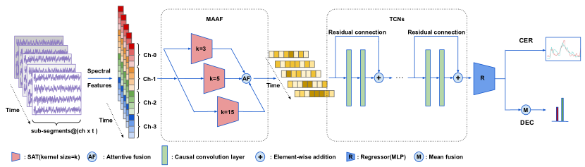
Figure 1: The architecture of our MASA-TCN. There are four main parts of MASA-TCN: feature extraction block, MAAF block, TCN block, and regression/classification block. A sequence of five four-EEG-channel sub-segments is utilized as an example. The k of SAT refers to the length of the kernel in the temporal dimension. Best viewed in color.

2 Preliminaries

2.1 Problem formulation

There are two types of EEG emotion recognition tasks to be addressed in this paper: CER and DEC. We provide a more formal description on the data annotation of CER and DEC. Given $N$ trials of continuous EEG signal $[\textbf{X}_{0},...,\textbf{X}_{N-1}],\textbf{X}\in\mathbb{R}^{C\times T}$, where $C$ is the number of EEG electrodes, $T$ is number of the temporal data points. Typically, the entire trial will be cut into shorter segments, denoted by $\bar{\textbf{X}}_{i},i\in[0,1,...,n-1]$, using a sliding window with or without overlap to train the neural networks. For CER, the labels are $\textbf{y}_{CER}=[\textbf{y}_{0},...,\textbf{y}_{n-1}],\textbf{y}\in\mathbb{R}^{1\times T/f_{s}^{y}}$, where $f_{s}^{y}$ is the sampling rate of the continues labels. Because the label of each trial in CER is continuous in the temporal dimension, the label is also cut into shorter segments as is done for the EEG data. The target of CER is to learn $f(\Theta):\textbf{X}_{i}\to\textbf{y}_{CER}$, which can:

$$\underset{\Theta}{argmin}\sum_{n-1}^{i=0}\Psi(f(\textbf{X}_{i}),\textbf{y}_{CER,i}),$$ (1)

where $\Theta$ is the trainable parameters of $f(\cdot)$ and $\Psi(\cdot)$ is the regression loss.

For DEC, the labels are $y_{DEC}=[y_{0},...,y_{n-1}],y\in\mathbb{R}$. Because there is one label for each trial in DEC, all the segments within one trial share the same label. The target of DEC is to learn $f(\Theta):\textbf{X}_{i}\to y_{DEC}$, which can:

$$\underset{\Theta}{argmin}\sum_{n-1}^{i=0}\Upsilon(f(\textbf{X}_{i}),y_{DEC,i}),$$ (2)

where $\Theta$ is the trainable parameters of $f(\cdot)$ and $\Upsilon(\cdot)$ is the cross-entropy loss.

2.2 Spatial-temporal patterns in EEG signals

EEG data have two-dimensional patterns: spatial and temporal patterns. EEG can be regarded as 2D time series, whose dimensions are channel and time.

The channel dimension consists of different EEG electrodes. The human brain has several functional areas that are related to different cognitive processes. A well-known definition of the brain functional areas is that the brain has frontal, parietal, occipital, and temporal lobes [27]. Different functional areas are not independently activated during the high-level cognitive processes, such as language [28] and emotion [29]. Because the electrodes are located in different functional areas of the brain, the channel dimension can reflect the relations among those functional areas.

The time dimension reflects the changes in brain activities from time to time. Emotions are continuous cognitive processes that vary in duration from a few seconds to several hours [30]. Usually, the stimulus in one trial of emotion-inducing experiments lasts from one to several minutes. The entire trial is cut into shorter segments with or without overlapping. For the DEC tasks, each segment is one sample, and all the segments within one trial share one label. Hence, neural networks need to capture spatial and short-term temporal patterns within each segment in order to infer. However, for the CER tasks, different segments within each trial have different labels, and the labels are continuous in the temporal dimension. Hence, neural networks need to capture the long-term temporal relations among each segment to do the regression.

EEG signals in different frequency bands have different relations to emotion [1]. Normally, the EEG signals are band-passed into several frequency bands, delta (1–3 Hz), theta (4–7 Hz), alpha (8–12 Hz), beta (13–30 Hz), and gamma ($>$30Hz) to analyze the brain activities from spectral information of EEG [31]. The EEG signals in different frequency bands are utilized to extract common spatial patterns (CSP) [32] or they are used to calculate different spectral features, such as PSD/rPSD [5] and DE [10]. This paper follows [9] that used rPSD as the spectral features for each shorter segments.

2.3 Neural networks for temporal pattern recognition

Two types of neural networks for temporal pattern recognition are introduced in this section: RNN and TCN. Different from the feed-forward neural networks, RNN takes the output of the previous step as the input to the next step and the temporal dynamics can be learned with the help of the internal hidden states. Among RNNs, LSTM [33] is one of the most commonly used neural networks for temporal sequential patterns modeling. LSTM uses a cell state to memorize the sequential information along the given data sequences. Several gates inside the LSTM cell project the input to hidden representations and control what information should be updated or forgotten. LSTM can be bidirectional that takes the input in opposite sequence orders to better learn the sequential pattern. GRU [34] is a simplified version of LSTM that has fewer gate operations while maintaining performance. With the temporal learning ability, LSTM was utilized in [26] to extract temporal patterns among the flattened PSD vectors along the time dimension for CER. TCN was proposed for action segmentation and detection in [35]. As a new class of temporal models, TCN uses causal convolutions and a stack of dilated convolutions to model the sequential information in a given temporal sequence. Residual connections were added into TCN [36] to further improve the temporal modeling ability of TCN. Zhang et. al., [9] applied TCN on CER using rPSD as features achieving the SOTA performance against LSTM [26].

Although the temporal dynamic patterns are extracted using LSTM and TCN, the spatial relations among different electrodes are not extracted effectively. Because all these previous methods use flattened spectral features as the input of LSTM and TCN. To enable TCN to learn spatial pattern effectively for the CER task, we design a space-aware temporal convolutional layer. Because emotion changes during the entire trial in different time scales [30, 37], a multi-anchor attentive fusion block is further proposed to improve the modeling ability of the temporal dynamics in the affective EEG data. Different from the works that use the learned representation by multiple dilation rates, we use different lengths of 1D causal convolutional kernels to model the dynamic temporal dependencies underlying emotional processes.

3 Method

In this section, the detailed introduction of each functional component in multi-anchor space-aware temporal convolutional neural networks (MASA-TCN) is presented. TCN has superior sequential pattern modeling ability. However, EEG data has spatial and temporal patterns to be extracted for the regression and classification tasks. Previous works use flattened rPSD features as the input to TCN directly, which can not extract the spatial pattern effectively. A space-aware temporal convolutional layer (SAT) is proposed to extract spatial-spectral patterns of EEG using TCN. Besides, to better learn the temporal dynamics underlying emotional cognitive processes that might appear in different time scales, we design a multi-anchor attentive fusion block (MAAF). The MAAF consists of three parallel SATs with different lengths of 1D causal convolution kernels. The outputs of these parallel SATs are attentively fused as the input to several TCN layers which learns the higher-level temporal patterns and generates the final hidden embedding. For the CER tasks, a linear layer is utilized as a regressor to map the hidden embedding to the continuous labels. For the DEC tasks, because these segments in time order share one label of that trial, a sum fusion layer is utilized to generate the final output instead of using a linear layer to get a single output. The overview of the proposed MASA-TCN is shown in Fig.  1.

3.1 Input construction

The construction of the network input is illustrated first to better understand the algorithm. As mentioned in Section 2.1, the EEG data of each trial is cut into shorter segments. Note that the sampling rates of the EEG data and continuous label are different, the former is much higher than the latter, e.g. 256Hz vs 4Hz in MAHNOB-HCI. Then the segments are further segmented into sub-segments along temporal dimension using a sliding window with a certain overlap to make sure the sub-segments are synchronized to each value of the continuous label for CER. For each sub-segment, it is still a 2D matrix, which has spatial and temporal dimensions. Because the sub-segments are in time orders, they can be regarded as frames in a video. For each sub-segments, averaged rPSDs in 6 frequency bands are calculated as [9]. We flatten the rPSDs along the EEG channel dimension, resulting in a feature vector:

$$\textbf{v}=[[p_{c_{0},f_{0}},...,p_{c_{0},f_{F-1}}],...,[p_{c_{C-1},f_{0}},...,p_{c_{C-1},f_{F-1}}]],$$ (3)

where $p$ is the averaged rPSD, $C$ is the total number of EEG channels, $F$ is the total number of the frequency bands, and $[\cdot]$ is the concatenation. Hence, one input to the neural networks would be:

$$\textbf{x}=[\textbf{v}_{0},...,\textbf{v}_{t-1}]^{T},$$ (4)

where t is the total number of the rPSD vectors within one segment.

TCN utilizes 1D CNN along the temporal dimension and treats the feature vector that contains spectral and spatial patterns as the channel dimension of 1D CNN. Hence, the spectral patterns across EEG channels as well as the spatial patterns of EEG channels are not effectively extracted. Instead of treating the feature vector dimension as the channel dimension of 1D CNN, we treat the input to TCN as a 2D matrix, whose dimensions are feature and time.

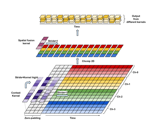
Figure 2: Space-aware temporal convolutional layer. The SAT has two types of convolutional kernels: context kernels that extract the spectral patterns channel by channel and spatial fusion kernels that learn spatial patterns across all the channels. A context kernel of size (4, 3) is utilized for example. And a four-EEG-channel sample with four spectral features in each EEG channel is used as the example. Zero padding is added to make the context kernel a causal kernel along temporal dimension. Only one kernel for each type of CNN kernels is shown in the diagram for better view, the final output (on the top) consists of the outputs from more kernels (4 is utilized as the number of kernels of each type for demonstration purpose). Best viewed in color.

3.2 Space-aware temporal convolutional layer

The SAT has two types of convolutional kernels: context kernels that extract the spectral patterns channel by channel and spatial fusion kernels that learn spatial patterns across all the channels. The structure of SAT is shown in Fig. 2.

Given the input $\textbf{x}=[\textbf{v}_{0},...,\textbf{v}_{t-1}]^{T},\textbf{v}\in\mathbb{R}^{1\times C*f}$ introduced in Section 3.1, the first type of the CNN kernels in SAT is the 2D causal convolutional kernel whose size, step, and dilation are $(f,k),(f,1)$, and $(1,2)$, where $f$ is the number of frequency bands used to calculate rPSDs and $k$ is the length of the CNN kernel in temporal dimension. Note that, the default dilation step is 1 instead of 0 in PyTorch [38] library, which means there is no dilation in that dimension if the dilation step is set as 1. Because the step in the feature dimension is the same as the height of the kernel, it can learn spectral contextual patterns across EEG channels. Hence, it is named as context kernel. The context kernel can learn spectral patterns as well as temporal dynamics at the same time due to its 2D shape. Different from WaveNet [39] that has dilation steps of $1,2,4,...2^{n-1}$, where n is the number of layers, as the first layer of MASA-TCN, it has a dilation of 2 in the temporal dimension. There are two reasons. The first reason is that the higher dilation step helps to get more discriminative information, considering the fact that the rPSD is calculated using overlapped sliding windows so that the adjacent vectors are highly correlated. The second reason is that discarding the TCN layer with a dilation step of 1 leads to smaller model size, without any compromises on the receptive field. Due to the causal convolution, the temporal dimension of the input and output are the same. Hence, we can get the output $\textbf{H}_{context}\in\mathbb{R}^{s,C,t}$, where $s$ is the number of context kernels, $C$ is the number of EEG channels, and $t$ is the total number of the rPSD vectors within one segment. $\textbf{H}_{context}$ can be calculated by:

$$\textbf{H}_{context}= Conv2D($$ (5)

$$input=\textbf{x},$$

$$kernel\_size=(f,k),$$

$$strides=(f,1),$$

$$dilation=(1,2)),$$

where $Conv2D$ is the 2D convolution with the input being x, the $kernel\_size,strides$, and $dilation$ are the parameters for the CNN operation. Note that the parameters are set as the default value in the PyTorch library unless otherwise specified.

The output of the context kernels is spatially fused by spatial fusion kernels to learn the spatial patterns of EEG channels. The size, stride, and dilation of the spatial kernels are $(C,1),(1,1),(1,1)$ respectively. This is the same as the commonly used spatial kernels of CNNs in BCI domains [11, 13]. Besides, it can be treated as an attentive fusion of all the EEG channels with the weights of the 1D CNN kernel being the attention scores. After $s$ spatial fusion kernels, the size of the hidden embedding $\textbf{H}_{SF}$ becomes $(s\times 1\times t)$. This process can be described as:

$$\textbf{H}_{SF}=Conv2D(\textbf{x},kernel\_size=(C,1)),$$ (6)

where the default value of strides $(1,1)$ and dilation $(1,1)$ are utilized.

3.3 Multi-anchor attentive fusion block

There are two steps in the MAAF: 1) parallel SATs with different temporal kernel lengths and 2) attentive fusion of the output from these SATs. The architecture of MAAF is shown in Fig. 1. TSception [8] utilizes multi-scale temporal convolutional kernels to capture temporal dynamics that might happen in different time scales. Emotion varies from time to time, especially for longer duration [37]. The duration of emotions varies from a few seconds to several hours [30].

Three parallel SATs with different temporal kernel sizes are utilized to capture those temporal dynamics in different time scales. In this paper, the temporal lengths of the context kernels are $k=[3,5,15]$ respectively. The longer the temporal length, the larger the temporal receptive field. Because the weights of the context kernels are distributed along the time dimension with the help of dilation steps, each weight is like an anchor on the time axis. Hence, we name these parallel SATs multi-anchor SATs. Besides, from the causal dependence perspective, different temporal kernel sizes can involve different previous results to decide the next output. We hypothesize that it can increase the robustness of the causal dependence in the temporal dimension underlying the continuous emotional cognitive process. The results in ablation studies also support the effectiveness of the multi-anchor design. The multi-anchor SATs can be described as:

$$\textbf{H}_{MA}^{i}=SAT(\textbf{x},kernel=(f,k_{i})),i\in[0,1,2],$$ (7)

where SAT contains the sequential operation of Eq. 5 and Eq. 6.

Different from TSception that directly concatenates the output of different scale kernels, an attentive fusion operation is adopted to combine the output from different SATs. First, the three outputs are concatenated along the kernel dimension (channel dimension of CNNs). A one-by-one convolutional layer serves as an attentive fusion layer as well as a dimension reducer that can reduce the concatenated dimensions back to the previous size, in our case, reducing the kernel dimension from $3*s$ to $s$. Hence, the output of the attentive fusion layer can be described as:

$$\textbf{H}_{AF}=Conv2D([\textbf{H}_{MA}^{0},\textbf{H}_{MA}^{1},\textbf{H}_{MA}^{2}],kernel\_size=(1,1)),$$ (8)

where $[\cdot]$ is the concatenation along the kernel dimension.

3.4 Temporal Convolutional layer

TCNs are further stacked to learn the temporal dependencies on top of the learned space-aware temporal patterns from MAAF. TCNs learn from temporal sequences by stacking causal convolution layers with the help of dilated 1D CNN kernels and residual connections [39]. A TCN can be described as:

$$\textbf{H}^{m}=TCN(\textbf{H}^{m-1})=\Phi(\textbf{H}^{m-1}+\sum_{i=0}^{k-1}f(i)\cdot\textbf{H}^{m-1}_{strd-d\cdot i}),$$ (9)

where $m$ is the layer index, $f(\cdot)$ is the filter, $k$ is the kernal size, $strd$ is stride, and $d$ is the dilation. $strd-d\cdot i$ is the direction of the past.

By stacking layers of TCNs, the temporal receptive field can be increased. The receptive field size can be calculated by:

$$F(m)=F(m-1)+2\times(k-1)\times d_{m},$$ (10)

where $m$ is the number of the convolutional block with residual connection, $k$ is the kernel size, $d_{m}$ is the dilation of the m-th convolutional block with the residual connection. When the dilation factor increases exponentially by $2$ as the number of TCN layers increases, the receptive field can be calculated as:

$$F(m)=1+2\cdot(k-1)\cdot\sum_{i=0}^{m-1}2^{i}=1+2\cdot(k-1)\cdot(2^{m}-1).$$ (11)

Because SAT, the first layer of MASA-TCN, has dilation of 2, the receptive field of MASA-TCN can be calculated as:

$$\bar{F}(m)=F(m+1)-k+1=1+(k-1)(2^{m+2}-3).$$ (12)

4 Experiments

4.1 Datasets

Two publicly availabel datasets are utilized in this paper: MAHNOB-HCI [6] for CER and DEAP [5] for DEC.

MAHNOB-HCI is a multi-model dataset to study human emotional responses and the implicit tagging of emotions. 30 subjects participated in the data collection experiments. Each subject watched 20 film clips, during which the synchronized recording of multi-angle facial videos, audio signals, EOG, EEG, respiration amplitude, and skin temperature were recorded. A subset [26] of the MAHNOB-HCI database that contains 24 participants’ 239 trials and the continuous labels in valence from several experts was utilized for the CER task. The averages of the experts’ annotations were taken as the final labels. The EEG signals have 32 electrodes and the sampling rate is 256 Hz. The annotations are of 4 Hz resolution.

DEAP is a multi-modal human affective states dataset. 32 subjects participated in the experiments. Each of them watched 40 1-min-long music videos while their EEG, facial expressions, and galvanic skin response (GSR) were recorded simultaneously. Self-assessments on arousal, valence, dominance, and liking from the subjects were utilized as the labels. A continuous 9-point scale was adopted to measure the level of those dimensions which was projected into low and high classes using a threshold of 5. Valence dimension was utilized in DEC task to be consistent with CER task. The EEG signals have 32 channels and the sampling rate is 512 Hz.

4.2 Preprocessing

For MAHNOB-HCI, the pre-processing steps are the same as [9]. For each trial of EEG, the first and last 30s’ non-stimuli durations of the data are removed after which average reference is conducted. The entire trial is split into shorter segments using a 2s’ sliding window with 0.25s’ overlap. Then the average rPSD of (0.3-5Hz), (5-8Hz), (8-12Hz), (12-18Hz), (18-30Hz), and (30-45Hz) is calculated using Welch’s method. By doing so, the 32 × 6 = 192-D rPSD features which have a frequency of 4Hz can be synchronized with the continuous labels. When training the neural networks, another sliding window with a length of 96 and a step size of 32 is applied to get the temporal sequence of the calculated rPSD vectors as [9]. Hence the size of the input to the neural networks is (batch, 192, 96).

For DEAP, we follow [8] to do the same pre-processing steps. For each trial of EEG, the first 3s’ baseline is removed. The data is downsampled to 128 Hz. EOG was removed as [5]. A band-pass filter from 4Hz to 45Hz is applied to remove low and high-frequency noise. Average reference is then conducted. Because MASA-TCN is designed for regression, it needs to learn from a temporal sequence of rPSD vectors. Each trial of EEG is split into 8s’ longer segments with 4s’ overlap as the temporal sequence to apply MASA-TCN on the DEC task and compare it with the SOTA DEC methods that take a shorter segment of EEG as input. Then the longer segments are further split into 2s’ shorter segments with 0.25s’ overlap to get the rPSDs in (0.3-5Hz), (5-8Hz), (8-12Hz), (12-18Hz), (18-30Hz), and (30-45Hz) six frequency bands. Note that the segment length in [8] is 4s, for a fair comparison, we rerun all the compared methods using 8s’ segments with 4s’ overlap.

4.3 Evaluation Metrics

The evaluation metrics for CER are the same as [9], they are root mean square error (RMSE), Pearson’s correlation coefficient (PCC), and concordance correlation coefficient (CCC). Given the prediction $\hat{\textbf{y}}$, and the continuous label y, RMSE, PCC, and CCC can be calculated as:

$$RMSE=\left\|\frac{\hat{\textbf{y}}-\textbf{y}}{N}\right\|^{2}=\sqrt{\frac{\sum_{N-1}^{i=0}(\hat{y}_{i}-y_{i})^{2}}{N}},$$ (13)

$$PCC=\frac{\sigma_{\hat{\textbf{y}}\textbf{y}}}{\sigma_{\hat{\textbf{y}}}\sigma_{\textbf{y}}}=\frac{\sum_{N-1}^{i=0}(\hat{y}_{i}-\mu_{\hat{\textbf{y}}})(y_{i}-\mu_{\textbf{y}})}{\sqrt{\sum_{N-1}^{i=0}(\hat{y}_{i}-\mu_{\hat{\textbf{y}}})^{2}}\sqrt{\sum_{N-1}^{i=0}(y_{i}-\mu_{\textbf{y}})^{2}}},$$ (14)

$$CCC=\frac{2\sigma_{\hat{\textbf{y}}\textbf{y}}}{\sigma_{\hat{\textbf{y}}}^{2}+\sigma_{\textbf{y}}^{2}+(\mu_{\hat{\textbf{y}}}-\mu_{\textbf{y}})},$$ (15)

where $N$ is the number of elements in the prediction/label vector, $\sigma_{\hat{\textbf{y}}\textbf{y}}$ is the covariance, $\sigma_{\hat{\textbf{y}}}$ and $\sigma_{\textbf{y}}$ are the variances, and $\mu_{\hat{\textbf{y}}}$ and $\mu_{\textbf{y}}$ are the means.

The RMSE can measure the point-to-point distances but the correlation between two vectors. The PCC can measure the correlation of two vectors ignoring the absolute point-to-point distances. CCC can take both correlation and point-to-point distances simultaneously which makes it a better evaluation metric for regression tasks.

The evaluation metrics for DEC are the same as [8]: accuracy (ACC) and F1 score. The calculating formulas of accuracy and F1 score are illustrated as follows:

$$ACC=\frac{TP+TN}{TP+FP+TN+FN},$$ (16)

$$F1=\frac{TP}{TP+\frac{1}{2}(FP+FN)},$$ (17)

where $TP$ is the true positive, $TN$ is the true negative, and $FP$ is the false positive, and $FN$ is the false negative.

4.4 Experiment Settings

For CER tasks, leave one subject out (LOSO) is utilized as [9]. For LOSO, one subject’s data are selected as test data, and the remaining subjects’ data are training data. Among the training data, 80% are randomly selected as training data, and the rest 20% are utilized as validation data. We repeat this process until each subject has been the test subject once. The mean RMES, PCC, and CCC are reported as the final results.

For DEC tasks, trial-wise 10-fold cross-validation is utilized as [8]. Emotion is one of the continuous cognitive processes. The adjacent segments within each trial are highly correlated. Randomly shuffling the segments among different trials before the training-test split can cause test data leakage. Because the highly correlated adjacent segments within each trial appear in both training and test set [8]. To avoid such data leakage issues and use a generalized evaluation setting, we use trial-wise randomization to divide each subject’s trials into ten folds as [8]. In each step of 10-fold cross-validation, one fold is utilized as test data, then 80% and 20% of the remaining nine folds are divided into training and validation data. The mean ACC and F1 of all the subjects are reported as the final results.

4.5 Implementation Details

For the CER task, we follow the same training strategy of [9]. CCC loss is utilized to guide the training.

$$\mathcal{L}_{CCC}(\hat{\textbf{y}},\textbf{y})=1-CCC(\hat{\textbf{y}},\textbf{y}).$$ (18)

The Adam optimizer with the initial learning rate of 1e-4, the weight decay of 1e-4 is utilized to train the network. ReduceLROnPlateau learning rate scheduler with a patient of 5, a reducing factor of 0.5 is used as well. The maximum training epoch is set as 15 and the early stopping patient is set as 10. The batch size is set as 2. The kernel size of MASA-TCN is set as [3, 5, 15]. We tune the depth and width of MASA-TCN based on the overall performance on validation data. When the depth is 2 and the width is 64, MASA-TCN gives the best results on validation data. The dropout rate is set as 0.15 for TCNs and 0.4 for RNNs (RNN, LSTM and GRU) as suggested in [26]. For baseline methods, we all use the same training strategy and parameters as the ones of MASA-TCN for fair comparison. We also compare our results with the ones reported in the existing literatures for the same task.

For the DEC task, based on the training strategy in [8], we further reduce the maximum training epochs from 500 to 100 and add early stopping with the patient being 10 to avoid over-fitting. Besides, a two-stage training strategy is adopted. It contains two stages. In stage I, we train the model using training data and evaluate it on the validation data. The model with the best validation ACC is saved. In stage II, we combine the training and validation data as new training data and re-train the saved model on the combined dataset for at maximum 50 epochs and stop training when the training loss reaches the stopping criteria. During the training stage, the training loss of the epoch with best validation ACC is saved as the stopping criteria in the second stage. The learning rate is 1e-3 and the batch size is 32. The dropout of TCN is still 0.15 because there is a dropout operation in every TCN layer. However is it too small for the baseline methods. Hence the dropout of baseline methods is still 0.5 which is suggested in [8]. Label-smoothing with a factor of 0.1 is added to further overcome the over-fitting problems. The depth and width of MASA-TCN are set as 3, and 16 based on the performance on validation data. The kernel size of MASA-TCN is still [3, 5, 15]. All the baselines are re-trained using the same training strategy and the same segment length of data as MASA-TCN for a fair comparison.

5 Results and Analysis

In this section, we first report the CER results of MASA-TCN against several baselines as well as the SOTA restuls reported in the recently published paper [9]. Then the ablation study results are presented to analyze the contribution of each functional component of MASA-TCN. After that, four types of analysis experiments are conducted to analyze the effects of 1) the starting dilation, 2) the model depth and width, 3) different fusion strategies in MAAF, and 4) early and late spatial learning. Lastly, the results for DEC tasks and the effect of mean fusion in last fully-connected layer are reported.

5.1 CER results on MAHNOB-HCI

We first compare the proposed MASA-TCN with several temporal learning neural networks then the CER results of MASA-TCN are compared with the SOTA results reported in the existing literature [9] that use the same experiment settings. Table I shows the CER results of RNN, LSTM, GRU, TCN, and MASA-TCN under the LOSO experiment setting. Table II lists down the reported SOTA results and the ones of MASA-TCN.

As shown in Table I, MASA-TCN achieves the best RMSE, PCC, and CCC on both validation and test sets among all the compared methods. MASA-TCN achieves a relative 14.29% (the absolute drop is 0.01) lower RMSE, a 0.043 higher PCC, and a 0.046 higher CCC than TCN. Compared with the RNN family, MASA-TCN also has a relative 10.45% (the absolute drop is 0.007) lower RMSE, a 0.015 higher PCC, and a 0.031 higher CCC than LSTM which is the best method among those RNNs. It is also observed that the RMSE of MASA-TCN on test and validation sets are consistent while the PCC and CCC have 0.06 and 0.128 gaps between validation and test set. This is because the subject-to-subject variance in the LOSO experiment setting and RMSE may not be a good indicator of regression compared with PCC and CCC. Compared with the SOTA results reported in the recently published paper [9] that uses the same experiment setting of CER (shown in Table II), MASA-TCN gets a relative 9.09% (the absolute drop is 0.006) lower RMSE, a 0.033 higher PCC, and a 0.04 higher CCC than the results reported by Zhang et. al. [9]. And MASA-TCN achieves a relative 25.93% (the absolute drop is 0.021) lower RMSE, a 0.08 higher PCC, and a 0.111 higher CCC than Soleymani’s methods reported in [9].

TABLE I: CER Results of LOSO on MAHNOB-HCI.

Method RMSE $\downarrow$ PCC $\uparrow$ CCC $\uparrow$ RNN 0.072$\pm$0.028 0.460$\pm$0.246 0.360$\pm$0.230 LSTM 0.067$\pm$0.028 0.492$\pm$0.242 0.386$\pm$0.245 GRU 0.071$\pm$0.033 0.470$\pm$0.236 0.382$\pm$0.238 TCN 0.070$\pm$0.027 0.464$\pm$0.246 0.371$\pm$0.262 MASA-TCN 0.060$\pm$0.023 0.507$\pm$0.219 0.417$\pm$0.236

• $\downarrow$: the lower the better; $\uparrow$: the higher the better.

TABLE II: Comparison with the results reported in the existing literature [9] using the same experiment setting for CER on MAHNOB-HCI.

Method RMSE $\downarrow$ PCC $\uparrow$ CCC $\uparrow$ Soleymani et. al. [26] 0.081$\pm$0.034 0.427$\pm$0.267 0.306$\pm$0.257 Zhang et. al. [9] 0.066$\pm$0.025 0.474$\pm$0.267 0.377$\pm$0.250 MASA-TCN 0.060$\pm$0.023 0.507$\pm$0.219 0.417$\pm$0.236

• $\downarrow$: the lower the better; $\uparrow$: the higher the better.

5.2 Ablation studies

Several ablation studies are conducted to understand how each component of MASA-TCN contributes to the improvements of CER results. Starting from the baseline TCN, SAT and MAAF are gradually added to see the effects of them. The results are shown in Table III.

According to Table III, adding SAT and MAAF can incrementally improve all the three metrics. By adding SAT along, the performances of TCN can be improved by relative 11.43% on RMSE, 0.022 on PCC, and 0.023 on CCC. The results are further improved from 0.062 to 0.060 on RMSE, from 0.486 to 0.507 on PCC, and from 0.394 to 0.417 when MAAF is also added. The results indicate the effectiveness of all those functional blocks in MASA-TCN.

TABLE III: Ablation study results of MASA-TCN on MAHNOB-HCI.

Method RMSE $\downarrow$ PCC $\uparrow$ CCC $\uparrow$ TCN 0.070$\pm$0.027 0.464$\pm$0.246 0.371$\pm$0.262 TCN+SA 0.062$\pm$0.023 0.486$\pm$0.214 0.394$\pm$0.230 TCN+SA+MA 0.060$\pm$0.023 0.507$\pm$0.219 0.417$\pm$0.236

• SA: Space-aware temporal convolutional layer; MA: Multi-anchor attentive fusion block.

• $\downarrow$: the lower the better; $\uparrow$: the higher the better.

5.3 Effect of the starting dilation

In this section, the effects of the starting dilation in the SAT are discussed. As mentioned in Section 3.2, the dilation of SAT starts from 2 instead of 1 which is used in TCN. There are two reasons. First, the EEG sub-segments are overlapped to synchronize them with the continuous labels, leading to some redundant information in the adjacent sub-segments. Using higher dilation at the SAT can learn the discriminative patterns effectively. Second, higher starting dilation in SAT can increase the receptive field which can reduce the number of TCN layers to get the same temporal receptive field, resulting in a more compact model size. To evaluate those effects, the starting dilation of SAT in MASA-TCN is set to 1, 2, and 4. The results are shown in Table IV.

TABLE IV: Effect of first-layer dilation of MASA-TCN on MAHNOB-HCI.

Dilation RMSE $\downarrow$ PCC $\uparrow$ CCC $\uparrow$ 1 0.063$\pm$0.025 0.494$\pm$0.224 0.401$\pm$0.237 2 0.060$\pm$0.023 0.507$\pm$0.219 0.417$\pm$0.236 4 0.062$\pm$0.022 0.499$\pm$0.220 0.411$\pm$0.243

• $\downarrow$: the lower the better; $\uparrow$: the higher the better.

The results show that increasing the dilation to a certain degree can improve the performance, and further increase of dilation can not provide gains on the CER results. When the dilation of SAT is 2, MASA-TCN has the best performance on both validation and test set. When the value is increased further to 4, the results slightly drop on both validation and test set. The possible reasons are a dilation of 2 and a TCN layer of 2 can give enough temporal receptive field and increase more can loss certain information among the adjacent sub-segments.

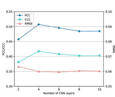
(a) Effect of the depth

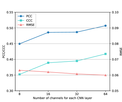
(b) Effect of the width

Figure 3: Effect of the depth and width of MASA-TCN.

5.4 Effect of the model depth and width

Experiments about the effects of model depth and width are conducted to better understand MASA-TCN. For model depth studies, the SAT is regarded as 2 layers due to the sequential operation of two types of CNN kernels. And there are 2 causal convolutional layers in one TCN layer. Hence the depths are set as 2, 4, 6, 8, and 10. For the width, it is the number of kernels in each CNN layer. The widths are set as 8, 16, 32, and 64. The results are shown in Fig. 3.

According to the results, depth is not sensitive when it is higher than 4, and the width more sensitively affects the model performance compared with the depth. From Fig. 3 (a), only having SAT and MAAF can not provide good performance. This is because the temporal receptive field is not enough. When the depth is 4, MASA-TCN achieves the best performance on both validation and test sets. However, when the depth increases to higher than 4, the performances drop a little bit and become stable. This is due to that enough temporal receptive field is achieved and a deeper model is relatively harder to train than the shallow one [40]. From Fig. 3 (b), the performances are positively related to the width. And when the width is 64, MASA-TCN achieves the best results on both validation and test sets. Note that we also conducted an experiment that use 128 as the width, but the model gave very low performances, which indicates the wider model is also harder to train.

5.5 Effect of different fusion strategies in MAAF

The effects of different fusion strategies in MAAF are analyzed and discussed in this section. Because three SATs with different kernel lengths are parallelly utilized in MAAF, the output needs to be fused for the subsequent TCNs. Three types of fusion mechanisms are studied: concatenation, mean, and attentive fusion.

Based on the results in Table V, all three types of fusion methods achieve relatively acceptable performances, and with attentive fusion, MASA-TCN has the best performances on both validation and test sets. This indicates the effectiveness of attention fusion in MAAF.

TABLE V: Effect of fusion strategy in MAAF on MAHNOB-HCI.

Fusion Method RMSE $\downarrow$ PCC $\uparrow$ CCC $\uparrow$ Concatenate 0.062$\pm$0.023 0.476$\pm$0.239 0.395$\pm$0.249 Mean 0.062$\pm$0.025 0.496$\pm$0.234 0.410$\pm$0.255 Attentive 0.060$\pm$0.023 0.507$\pm$0.219 0.417$\pm$0.236

• $\downarrow$: the lower the better; $\uparrow$: the higher the better.

5.6 Effect of early and late spatial learning

The order of spatial learning is studied in this part. As illustrated in Section 2.2, there are spatial, spectral, and temporal patterns that need to be recognized for EEG data. Typically the spatial patterns can be learned by a 1D CNN kernel whose size is $(c,1)$, where $c$ is the number of EEG channels. In MASA-TCN, the spatial learning is done in SAT, which is regarded as early spatial learning. The spatial patterns can also be learned after the last several TCN layers, which is termed late spatial learning. We compare both early and late spatial learning. The results are shown in Table VI.

Early spatial learning is more effective than late spatial learning according to the results. It is noticeable that late spatial learning can not even has comparable performance with the one using early spatial learning. More analyses should be done in the future to better understand the reason.

TABLE VI: Effect of early and late spatial learning of MASA-TCN on MAHNOB-HCI.

Spatial Learning RMSE $\downarrow$ PCC $\uparrow$ CCC $\uparrow$ Late 0.434$\pm$0.602 0.153$\pm$0.250 0.115$\pm$0.189 Early 0.060$\pm$0.023 0.507$\pm$0.219 0.417$\pm$0.236

• $\downarrow$: the lower the better; $\uparrow$: the higher the better.

5.7 DEC results on DEAP

MASA-TCN achieves SOTA performances on CER tasks, we further explore the possibility of extending it to DEC tasks and compare it with the SOTA methods of DEC tasks, SVM (2012) [5], DeepConvNet (2017) [11], EEGNet (2018) [13], , and TSception (2022) [8] in this section. Because MASA-TCN is mainly designed for CER tasks, a regressor is utilized to generate a 1D output that has the same length as the continuous labels. One way to adapt MASA-TCN to DEC is to change the output size of the regressor from 1D to binary output and the regressor becomes a normal classifier in most deep learning methods for classification. However, we can also extend MASA-TCN to DEC by using a mean fusion on the output of the regressor as a kind of classifier ensemble which can increase the robustness. Hence, in MASA-TCN, we choose the latter to extend it from the CER tasks to the DEC tasks. Note that for a fair comparison, all the methods use the same data preprocessing steps, the same segment length (8s) with a overlapping of 50%, and the same training strategies as the ones of MASA-TCN. The results are shown in Table VII.

As seen in Table VII, MASA-TCN achieves higher ACC and F1 Scores than the compared methods. It is observed that the difference of ACC among deep learning methods are not significant, while they all get a higher ACC compared with SVM. MASA-TCN has larger improvements over the compared methods in term of F1 scores. MASA-TCN has a 4.51% higher F1 Score than DeepConvNet, and the improvement over the one of EEGNet is 6.44%. The F1 score of TSception is 7.49% lower than the one of MASA-TCN. MASA-TCN improves the F1 score from 58.07% to 64.58% compared with SVM.

TABLE VII: Results of DEC task on DEAP.

Method	ACC(%)	F1(%)
SVM	55.17	58.07
EEGNet	58.45	58.14
DeepConvNet	59.30	60.07
TSception	58.71	57.09
MASA-TCN	60.20	64.58

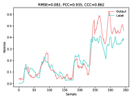
(a) Well regressed

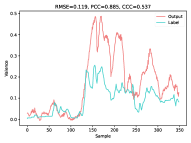
(b) Moderately regressed

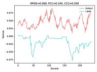
(c) Poorly regressed

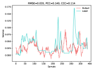
(d) Poorly regressed

Figure 4: Four representative samples of well and poorly regressed trials of MASA-TCN for CER

6 Discussion

The CER tasks are relatively more comprehensive to study human emotions. CER tasks require the model to predict the temporally continuous labels of emotions using EEG signals, which are rarely explored in the existing literatures [9]. Emotion is a continuous neural cognitive process of the brain [30]. In general EEG collection experiments in the studies for emotions [5, 6], the subjects are required to watch and listen to the affective stimuli for a certain duration. And the emotional states are not consistent during the entire trial [37]. By refining the label of shorter segments using the continuous label instead of the single label of one trial in DEC, improvements in classification are observed [41]. Despite the importance of exploring novel methods for EEG CER tasks, only a few works [9, 26] have proposed some algorithms. And all of them use flattened feature vectors as input while not effectively learning the spatial patterns across EEG channels.

MASA-TCN is proposed in this paper to enable TCN to learn spatial, spectral, and temporal patterns simultaneously for the CER tasks. The main functional block for spatial learning is the SAT layer that consists of context kernel and spatial fusion kernel two types of CNN kernels. With the help of zero padding and dilation along the temporal dimension, SAT can also learn the temporal causal dependencies. Because EEG contains abundant temporal information that is related to the brain’s emotional activities changes from time to time, and the temporal dependencies might happen in different time scales [8, 30], a MAAF block is further designed to capture those temporal dynamics with the help of multiple temporal kernel lengths as well as an attentive fusion layer. Extensive experiments on a publicly available dataset have been done to evaluate the proposed method. The results demonstrate the effectiveness of MASA-TCN for CER tasks and we set new SOTA results against the recently published results in [9]. We further extend MASA-TCN from regression tasks to classification tasks by adding a mean fusion in the final fully-connected layer (regressor). It also achieves higher classification results over several SOTA methods in DEC tasks. To the best of our knowledge, this is the first work to propose a unified model for both CER and DEC tasks. The experiment also indicates that calculating the mean of the output of a regressor as the classification output can yield a certain improvement in F1 scores.

Besides the analysis experiments we conducted and discussed in Section 5, some discussions on the output of MASA-TCN for CER are given here. Four representative samples for well, moderately, and poorly regressed trials are selected to show the differences between the prediction and ground truth. They are shown in Fig. 4. The discussions are two-fold: the performance of MASA-TCN for CER and the differences among the three evaluation metrics.

We first discuss the performance of MASA-TCN. According to Fig. 4 (a) and (b), MASA-TCN can well regress the relatively smaller absolute value ($>0.15$) while the predictions of larger-value labels, especially the ones with sudden changes, are not well addressed. In the future, some regularization terms can be added to the output of MASA-TCN to reduce the amplitude after sudden changes. It is also noticeable that MASA-TCN handles the positive labels better than the negative ones by comparing Fig. 4 (a), (b), and (c). Based on Fig. 4 (d), it can be seen that MASA-TCN can not well regress the details of sudden short-term fluctuations. RMSE can punish the distance between prediction and label point-wise, hence, it is worth trying to guide the training using a weighted combination of RMSE and CCC for better regression of the details instead of using CCC loss only. Next, we give some discussions on the evaluation metrics.

CCC is a better evaluation metric for CER compared with RMSE and PCC. RMSE focuses on point-to-point precision, while the correlation between the predictions and labels is not effectively measured. As shown in Fig. 4, when the trial is well regressed (Fig. 4 (a)), RMSE is still larger than the ones of the poorly regressed ones (Fig. 4 (c) and Fig. 4 (d)). That’s because the labels are in relatively lower amplitudes in Fig. 4 (c) and (d) than the ones in Fig. 4 (a). Even though the trends are not well regressed, the point-to-point distances are still small. However, CCCs of those two poorly regressed outputs are much lower than the well-regressed ones because CCC also measures the correlation between the two vectors. Although PCC can measure the correlations, it ignores the absolute distances among points of the outputs and labels. Hence, we can see the PCC is still high in Fig. 4 (b) even though there are long drifts between the outputs and labels. CCC can reflect those drifts as well, hence, the CCC of Fig. 4 (a) is much higher than the one of Fig. 4 (b).

There are also some limitations in this work that need to be discussed. The first one is the lack of datasets for CER tasks. This is a common problem for EEG CER tasks. Because preparing a dataset for the EEG CER tasks needs well-designed experiment protocols as well as the efforts of a number of experts to continuously annotate the corresponding trials. In the future, more datasets need to be created to further boost this research area. Besides, more interpretability methods should be applied to better understand why early spatial learning is much better than late spatial learning. At last, in this paper, we follow [9] that only uses CCC in the loss function to guide the training process. In the future, using a weighted combination of RMSE, PCC, and CCC in the loss function is expected to provide certain improvements.

7 Conclusion

In this paper, MASA-TCN is proposed to improve the SOTA results of the CER and DEC tasks using EEG. Compared with the SOTA methods [9, 26] that don’t effectively learn the spatial patterns among EEG channels, a novel SAT layer is designed to enable TCN to capture spatial, spectral, and temporal patterns simultaneously. A MAAF block is further proposed to capture the temporal dynamics that might happen in different time scales underlying emotional cognitive processes. By adding a mean fusion in the output of the regressor of MASA-TCN, we further extend MASA-TCN from CER to DEC, making it a unified model for both the CER and DEC tasks using EEG. Extensive experiments on two public emotion datasets show the effectiveness of the proposed methods for both CER and DEC. New SOTA results are achieved by MASA-TCN for those tasks.

References

- [1] S. M. Alarcão and M. J. Fonseca, “Emotions recognition using EEG signals: A survey,” IEEE Transactions on Affective Computing, vol. 10, no. 3, pp. 374–393, 2019.
- [2] Y. Li, Y. Wang, and Z. Cui, “Decoupled multimodal distilling for emotion recognition,” in Proceedings of the IEEE/CVF Conference on Computer Vision and Pattern Recognition (CVPR), June 2023, pp. 6631–6640.
- [3] R. J. Dolan, “Emotion, cognition, and behavior,” Science, vol. 298, no. 5596, pp. 1191–1194, 2002.
- [4] Y. Li, J. Zeng, S. Shan, and X. Chen, “Self-supervised representation learning from videos for facial action unit detection,” in Proceedings of the IEEE/CVF Conference on Computer Vision and Pattern Recognition (CVPR), June 2019.
- [5] S. Koelstra, C. Muhl, M. Soleymani, J.-S. Lee, A. Yazdani, T. Ebrahimi, T. Pun, A. Nijholt, and I. Patras, “DEAP: A database for emotion analysis using physiological signals,” IEEE Transactions on Affective Computing, vol. 3, no. 1, pp. 18–31, 2012.
- [6] M. Soleymani, J. Lichtenauer, T. Pun, and M. Pantic, “A multimodal database for affect recognition and implicit tagging,” IEEE Transactions on Affective Computing, vol. 3, no. 1, pp. 42–55, 2012.
- [7] S.-H. Hsu, Y. Lin, J. Onton, T.-P. Jung, and S. Makeig, “Unsupervised learning of brain state dynamics during emotion imagination using high-density EEG,” NeuroImage, vol. 249, p. 118873, 2022.
- [8] Y. Ding, N. Robinson, S. Zhang, Q. Zeng, and C. Guan, “TSception: Capturing temporal dynamics and spatial asymmetry from EEG for emotion recognition,” IEEE Transactions on Affective Computing, pp. 1–1, 2022.
- [9] S. Zhang, C. Tang, and C. Guan, “Visual-to-EEG cross-modal knowledge distillation for continuous emotion recognition,” Pattern Recognition, vol. 130, p. 108833, 2022.
- [10] W.-L. Zheng, J.-Y. Zhu, and B.-L. Lu, “Identifying stable patterns over time for emotion recognition from EEG,” IEEE Transactions on Affective Computing, vol. 10, no. 3, pp. 417–429, 2019.
- [11] R. T. Schirrmeister, J. T. Springenberg, L. D. J. Fiederer, M. Glasstetter, K. Eggensperger, M. Tangermann, F. Hutter, W. Burgard, and T. Ball, “Deep learning with convolutional neural networks for EEG decoding and visualization,” Human Brain Mapping, vol. 38, no. 11, pp. 5391–5420, 2017.
- [12] S. Sakhavi, C. Guan, and S. Yan, “Learning temporal information for brain-computer interface using convolutional neural networks,” IEEE Transactions on Neural Networks and Learning Systems, vol. 29, no. 11, pp. 5619–5629, 2018.
- [13] V. J. Lawhern, A. J. Solon, N. R. Waytowich, S. M. Gordon, C. P. Hung, and B. J. Lance, “EEGNet: a compact convolutional neural network for EEG-based brain–computer interfaces,” Journal of Neural Engineering, vol. 15, no. 5, p. 056013, jul 2018.
- [14] O.-Y. Kwon, M.-H. Lee, C. Guan, and S.-W. Lee, “Subject-independent brain–computer interfaces based on deep convolutional neural networks,” IEEE Transactions on Neural Networks and Learning Systems, vol. 31, no. 10, pp. 3839–3852, 2020.
- [15] Y. Ding, N. Robinson, C. Tong, Q. Zeng, and C. Guan, “Lggnet: Learning from local-global-graph representations for brain–computer interface,” IEEE Transactions on Neural Networks and Learning Systems, pp. 1–14, 2023.
- [16] Z. Jiao, X. Gao, Y. Wang, J. Li, and H. Xu, “Deep convolutional neural networks for mental load classification based on EEG data,” Pattern Recognition, vol. 76, pp. 582–595, 2018.
- [17] T. Zhang, W. Zheng, Z. Cui, Y. Zong, and Y. Li, “Spatial–temporal recurrent neural network for emotion recognition,” IEEE Transactions on Cybernetics, vol. 49, no. 3, pp. 839–847, 2019.
- [18] Y. Li, W. Zheng, L. Wang, Y. Zong, and Z. Cui, “From regional to global brain: A novel hierarchical spatial-temporal neural network model for EEG emotion recognition,” IEEE Transactions on Affective Computing, pp. 1–1, 2019.
- [19] T. Song, W. Zheng, P. Song, and Z. Cui, “EEG emotion recognition using dynamical graph convolutional neural networks,” IEEE Transactions on Affective Computing, vol. 11, no. 3, pp. 532–541, 2020.
- [20] X.-h. Wang, T. Zhang, X.-m. Xu, L. Chen, X.-f. Xing, and C. L. P. Chen, “EEG emotion recognition using dynamical graph convolutional neural networks and broad learning system,” in 2018 IEEE International Conference on Bioinformatics and Biomedicine (BIBM), 2018, pp. 1240–1244.
- [21] C. Li, B. Chen, Z. Zhao, N. Cummins, and B. W. Schuller, “Hierarchical attention-based temporal convolutional networks for EEG-based emotion recognition,” in ICASSP 2021 - 2021 IEEE International Conference on Acoustics, Speech and Signal Processing (ICASSP), 2021, pp. 1240–1244.
- [22] X. Xing, Z. Li, T. Xu, L. Shu, B. Hu, and X. Xu, “SAE+LSTM: A new framework for emotion recognition from multi-channel EEG,” Frontiers in Neurorobotics, vol. 13, 2019.
- [23] W. Tao, C. Li, R. Song, J. Cheng, Y. Liu, F. Wan, and X. Chen, “EEG-based emotion recognition via channel-wise attention and self attention,” IEEE Transactions on Affective Computing, pp. 1–1, 2020.
- [24] D. Kollias and S. Zafeiriou, “Analysing affective behavior in the second ABAW2 competition,” in 2021 IEEE/CVF International Conference on Computer Vision Workshops (ICCVW), 2021, pp. 3645–3653.
- [25] F. Ringeval, B. Schuller, M. Valstar, N. Cummins, R. Cowie, L. Tavabi, M. Schmitt, S. Alisamir, S. Amiriparian, E.-M. Messner, S. Song, S. Liu, Z. Zhao, A. Mallol-Ragolta, Z. Ren, M. Soleymani, and M. Pantic, “AVEC 2019 workshop and challenge: State-of-mind, detecting depression with AI, and cross-cultural affect recognition,” in Proceedings of the 9th International on Audio/Visual Emotion Challenge and Workshop, ser. AVEC ’19. New York, NY, USA: Association for Computing Machinery, 2019, p. 3–12.
- [26] M. Soleymani, S. Asghari-Esfeden, Y. Fu, and M. Pantic, “Analysis of EEG signals and facial expressions for continuous emotion detection,” IEEE Transactions on Affective Computing, vol. 7, no. 1, pp. 17–28, 2016.
- [27] T. Alotaiby, F. E. A. El-Samie, S. A. Alshebeili, and I. Ahmad, “A review of channel selection algorithms for EEG signal processing,” EURASIP Journal on Advances in Signal Processing, vol. 2015, no. 1, p. 66, 2015.
- [28] A. D. Friederici, N. Chomsky, R. C. Berwick, A. Moro, and J. J. Bolhuis, “Language, mind and brain,” Nature Human Behaviour, vol. 1, no. 10, pp. 713–722, 2017.
- [29] H. Kober, L. F. Barrett, J. Joseph, E. Bliss-Moreau, K. Lindquist, and T. D. Wager, “Functional grouping and cortical–subcortical interactions in emotion: A meta-analysis of neuroimaging studies,” NeuroImage, vol. 42, no. 2, pp. 998–1031, 2008.
- [30] P. Verduyn, P. Delaveau, J.-Y. Rotgé, P. Fossati, and I. V. Mechelen, “Determinants of emotion duration and underlying psychological and neural mechanisms,” Emotion Review, vol. 7, no. 4, pp. 330–335, 2015.
- [31] J. N. Saby and P. J. Marshall, “The utility of EEG band power analysis in the study of infancy and early childhood,” Developmental neuropsychology, vol. 37, no. 3, pp. 253–273, 2012.
- [32] K. K. Ang, Z. Y. Chin, H. Zhang, and C. Guan, “Filter bank common spatial pattern (FBCSP) in brain-computer interface,” in 2008 IEEE International Joint Conference on Neural Networks (IEEE World Congress on Computational Intelligence), 2008, pp. 2390–2397.
- [33] S. Hochreiter and J. Schmidhuber, “Long short-term memory,” Neural Computation, vol. 9, no. 8, pp. 1735–1780, 1997.
- [34] K. Cho, B. van Merrienboer, D. Bahdanau, and Y. Bengio, “On the properties of neural machine translation: Encoder-decoder approaches,” 2014.
- [35] C. Lea, M. D. Flynn, R. Vidal, A. Reiter, and G. D. Hager, “Temporal convolutional networks for action segmentation and detection,” in 2017 IEEE Conference on Computer Vision and Pattern Recognition (CVPR), 2017, pp. 1003–1012.
- [36] S. Bai, J. Z. Kolter, and V. Koltun, “An empirical evaluation of generic convolutional and recurrent networks for sequence modeling,” 2018.
- [37] Y. Zhang, H. Liu, D. Zhang, X. Chen, T. Qin, and Q. Zheng, “EEG-based emotion recognition with emotion localization via hierarchical self-attention,” IEEE Transactions on Affective Computing, pp. 1–1, 2022.
- [38] A. Paszke, S. Gross, F. Massa, A. Lerer, J. Bradbury, G. Chanan, T. Killeen, Z. Lin, N. Gimelshein, L. Antiga, A. Desmaison, A. Kopf, E. Yang, Z. DeVito, M. Raison, A. Tejani, S. Chilamkurthy, B. Steiner, L. Fang, J. Bai, and S. Chintala, “PyTorch: An imperative style, high-performance deep learning library,” in Advances in Neural Information Processing Systems 32. Curran Associates, Inc., 2019, pp. 8024–8035.
- [39] A. van den Oord, S. Dieleman, H. Zen, K. Simonyan, O. Vinyals, A. Graves, N. Kalchbrenner, A. Senior, and K. Kavukcuoglu, “WaveNet: A generative model for raw audio,” in ISCA Speech Synthesis Workshop (SSW), 2016.
- [40] K. He, X. Zhang, S. Ren, and J. Sun, “Deep residual learning for image recognition,” in 2016 IEEE Conference on Computer Vision and Pattern Recognition (CVPR), 2016, pp. 770–778.
- [41] S. Zhang and C. Guan, “Emotion recognition with refined labels for deep learning,” in 2020 42nd Annual International Conference of the IEEE Engineering in Medicine & Biology Society (EMBC), 2020, pp. 108–111.