images/
Collaborative Information Dissemination with Graph-based Multi-Agent Reinforcement Learning
Abstract
Efficient information dissemination is crucial for supporting critical operations across domains like disaster response, autonomous vehicles, and sensor networks. This paper introduces a Multi-Agent Reinforcement Learning (MARL) approach as a significant step forward in achieving more decentralized, efficient, and collaborative information dissemination. We propose a Partially Observable Stochastic Game (POSG) formulation for information dissemination empowering each agent to decide on message forwarding independently, based on the observation of their one-hop neighborhood. This constitutes a significant paradigm shift from heuristics currently employed in real-world broadcast protocols. Our novel approach harnesses Graph Convolutional Reinforcement Learning and Graph Attention Networks (GATs) with dynamic attention to capture essential network features. We propose two approaches, L-DyAN and HL-DyAN, which differ in terms of the information exchanged among agents. Our experimental results show that our trained policies outperform existing methods, including the state-of-the-art heuristic, in terms of network coverage as well as communication overhead on dynamic networks of varying density and behavior.
1 Introduction
Group communication, implemented in a broadcast or multicast fashion, finds a natural application in different networking scenarios, such as Vehicular Ad-hoc Networks (VANETs) Tonguz et al. (2007); Ibrahim et al. (2020), with the necessity to disseminate information about the nodes participating, e.g. identity, status, or crucial events happening in the network. These systems can be characterized by congestion-prone networks and/or different resource constraints, such that message dissemination becomes considerably expensive if not adequately managed. For this matter, message forwarding calls for scalable and distributed solutions able to minimize the total number of forwards, while achieving the expected coverage. Moreover, modern broadcast communication protocols often require careful adjustments of their parameters before achieving adequate forwarding policies, which would otherwise result in sub-optimal performance in terms of delivery ratio and latency Suri et al. (2022).
Recently, researchers have considered learning communication protocols Foerster et al. (2016) with Multi-Agent Reinforcement Learning (MARL) Buşoniu et al. (2010). At its core, MARL seeks to design systems where multiple agents learn to optimize their objective by interacting with the environment and the other entities involved. Such tasks can be competitive, cooperative, or a combination of both, depending on the scenario. As agents interact within a shared environment, they often find the need to exchange information to optimize their collective performance. This has led to the development of communication mechanisms that are learned rather than pre-defined, allowing agents to cooperate better utilizing their learned signaling system.
Nevertheless, learning to communicate with MARL comes with several challenges. In multi-agent systems, actions taken by one agent can significantly impact the rewards and state transitions of other agents, rendering the environment more complex and dynamic, and ensuring that agents develop a shared and consistent communication protocol, is an area of active research. Methods such as CommNet Sukhbaatar et al. (2016) and BiCNet Peng et al. (2017), focus on the communication of local encodings of agents’ observations. These approaches allow agents to share a distilled version of their perspectives, enabling more informed collective decision-making. ATOC Jiang and Lu (2018) and TarMAC Das et al. (2019) have ventured into the realm of attention mechanisms. By leveraging attention, these methods dynamically determine which agents to communicate with and what information to share, leading to more efficient and context-aware exchanges. Yet another approach, as exemplified by Graph Convolutional Reinforcement Learning (DGN) Jiang et al. (2020), harnesses the power of Graph Neural Networks (GNNs) and attention mechanisms to model the interactions, relations, and communications between agents.
However, to the best of our knowledge, no MARL-based method involving proactive communication and GNNs has been proposed to address the unique challenges of optimizing the process of information dissemination within a broadcast dynamic network. In such a scenario, nodes need to cooperate to spread the information by forwarding it to their immediate neighbors, which might change over time, while relying on their limited observation of the entire graph. Furthermore, their collaboration and ability to accomplish dissemination are bound by the limitations of the underlying communication channels. This means that both the quantity of forwarding actions and the amount of information exchange needed for effective cooperation are constrained and should be minimized.
Contributions
In this work, we introduce a novel Partially Observable Stochastic Game (POSG) for optimized information dissemination in dynamic broadcast networks, forming the basis for our MARL framework.111https://github.com/RaffaeleGalliera/melissa.
To this end, we design a MARL algorithm to encourage cooperation within dynamic neighborhoods where node connections are frequently changing. Furthermore, we design and test two distinct architectures, namely Local Dynamic Attention Network (L-DyAN) and Hyperlocal Dynamic Attention Network (HL-DyAN), which require different levels of communication leveraging Graph Attention Network (GAT) with dynamic attention Brody et al. (2022) and Dueling Q-Networks Wang et al. (2016).
Our experimental study demonstrates our methods’ efficacy in achieving superior network coverage across dynamic graphs in different scenarios, outperforming DGN and the established Multipoint Relay (MPR) Dearlove and Clausen (2014) heuristic. Moreover, our approach operates on one-hop observations and empowers nodes to take independent forwarding decisions, unlike MPR.
By exploring the potential of learning-based approaches for addressing information dissemination in dynamic networks, our work underscores the versatility of MARL in present and future, real-world applications such as information dissemination in social networks Guille et al. (2013), space networks Ye and Zhou (2021), and vehicle-safety-related communication services Ma et al. (2012).
2 Background
Reinforcement Learning (RL)
provides solutions for sequential decision-making problems formulated as Markov Decision Processs (MDPs) Sutton and Barto (2018); Puterman (1994). The Partially Observable Markov Decision Process (POMDP) extends the MDP framework to scenarios where agents have limited or partial observability of the underlying environment and make decisions based on belief states, which are probability distributions over the true states. To this end, several methods have been proposed such as Deep Recurrent Q-Learning Hausknecht and Stone (2015).
Multi-Agent Reinforcement Learning
For multi-agent systems the RL paradigm extends to MARL Buşoniu et al. (2010), where multiple entities, potentially learners and non-learners, interact with the environment. In this context the generalization of POMDPs leads to Decentralized Partially Observable Markov Decision Process (Dec-POMDP), characterized by the tuple . Here, represents the set of agents, denotes the state space, stands for the action space for each agent, is the joint probability distribution governing the environment dynamics given the current state and joint actions, denotes the reward function, and represents the set of observations for each agent. Such game-theoretic settings are used to model fully cooperative tasks where all agents have the same reward function and share a common reward.
A more general model, adopted in this work, is the Partially Observable Stochastic Game (POSG), where each agent receives an individual reward , allowing the definition of fully competitive and mixed tasks such as zero-sum and general-sum games Albrecht et al. (2023). Several MARL algorithms have been presented in the literature, addressing different tasks (cooperative, competitive, or mixed) and pursuing different learning goals such as stability or adaptation Buşoniu et al. (2010); Ahmed et al. (2022).
Graph Neural Networks
GNNs Scarselli et al. (2009) process graph structures, and enable predictions at the graph, node, or edge level. This is achieved by combining function approximators such as Neural Networks (NNs) with a Message Passing mechanism, where a node aggregates over the immediate neighbors’ features and combines its features with the aggregated information. Repeating this operation times convolves information over nodes hops away. GNNs have shown remarkable success in several domains, such as recommendation systems, drug discovery, and social network analysis. Recent advancements have introduced novel GNN architectures, such as Graph Convolutional Network (GCN) Kipf and Welling (2017), GraphSAGE Hamilton et al. (2017), and GAT Veličković et al. (2018), which have improved the performance on various tasks. In this paper, we use GATs with dynamic attention Brody et al. (2022) to capture relevant features of communication networks.
Graph Convolutional Reinforcement Learning
In DGN Jiang et al. (2020), the dynamics of multi-agent environments are represented as a graph, where each agent is a node with a set of neighbors determined by specific metrics. In this approach, a key role is played by Relation Kernels and their capability to merge features within an agent’s receptive field, which is increased with the number of graph convolutional layers, all while capturing detailed interactions and relationships between agents. Building upon this foundation, during training, a batch of experiences is sampled and the following loss is minimized:
| (1) |
where is the number of agents, and is the observation of agent with the respective adjacency matrix . We build on DGN and design novel MARL architectures for optimizing information dissemination in dynamic networks.
Optimized Flooding in Broadcast Networks
A dynamic broadcast network can be represented as a dynamic graph , where each node represents a (possibly) mobile node and an edge between two nodes at time represents the two corresponding nodes being within each other’s broadcasting range at that time. Hence, for every node , the set of its neighbors at time is defined as .
A main objective of broadcast communications over connected networks is called Optimized Flooding Qayyum et al. (2002) and it is achieved when the information emitted from a given node reaches every other node , thanks to forwarding actions of a set of nodes . While maximizing coverage it is also desirable to minimize redundant transmissions, which might impact resource utilization, such as bandwidth, power consumption, and latency. From a graph-theoretic point of view this can be achieved by identifying a specific subset of nodes, called a Minimum Connected Dominating Set (MCDS), that will be tasked with forwarding the information. This task requires the introduction of a centralized entity with complete knowledge of the network state and has been shown to be NP-complete Garey and Johnson (1979). A much more efficient and realistic approach is to approximate the MCDS in a distributed manner, relying only on local observations of the network made from each node’s perspective. Indeed, this is the approach taken by the MPR selection heuristic and our MARL approach.
3 Related Work
The MPR selection algorithm is a technique developed to efficiently disseminate information in Mobile Ad-hoc Networks (MANETs) and wireless mesh networks. It achieves this by having each node designate certain one-hop neighbors to forward messages arriving from them, thereby reducing the overall transmission load and preventing excessive network broadcasting. This process involves nodes exchanging “HELLO messages” to identify and select their MPR sets, ensuring effective network coverage with minimal redundancy.
In real-world networking protocols, MPR plays an essential role. For instance, in the Optimized Link State Routing (OLSR) protocol Dearlove and Clausen (2014), MPR is fundamental in managing the distribution of Topology Control (TC) messages. Similarly, in Simplified Multicast Forwarding (SMF) Macker (2012), MPR is employed primarily for the efficient forwarding of multicast packets.
In this work, we compare our approach with the MPR selection algorithm, as outlined in the standard OLSR implementation Dearlove and Clausen (2014), leveraging this algorithm as a baseline for distributed message dissemination in dynamic graph structures.222The complete MPR selection algorithm used by OLSR is shown in Algorithm 1-Appendix A.1 However, we define a completely different approach that leverages MARL and, unlike MPR, only requires an anonymized knowledge of the one-hop neighborhood and empowers each agent to independently decide their message forwarding policy.
Recent work has considered MARL approaches in the context of communication networks Yahja et al. (2022); Kaviani et al. (2021, 2023). The more closely related to the presented work is DeepMPR Kaviani et al. (2023) which addresses the optimization of specific networking metrics in the context of multicast networks. While related, both the problem considered and the approach taken here are different. In particular, we focus on coverage and forwarded message minimization rather than metrics such as goodput, which apply only to such domains. Moreover, in contrast to Kaviani et al. (2023) where the proposed method utilizes PPO Schulman et al. (2017) and policies trained with observation and action spaces tailored to specific graph scenarios, we design a more general approach, introducing a novel POSG with a dynamic number of participating agents and a scalable graph-based solution, which employs two novel approaches based on DGN and GAT with dynamic attention for capturing essential local features and relations among agents.
4 Method
In this section, we describe our novel MARL approach for optimizing information flooding in dynamic broadcast networks. We start by presenting a POSG formulation and then introduce our learning method and our two architectures, L-DyAN and HL-DyAN, designed to achieve efficient dissemination while requiring different degrees of communication.
4.1 MARL Formulation
We envision the dissemination process discretized into timesteps and episodes starting with a source node transmitting the information (a message) to its immediate (one-hop) neighbors. Each node in the graph corresponds to an agent observing its one-hop neighborhood and their features. At every timestep, nodes that have received the message will sense their neighborhood and decide whether to forward it to its current one-hop neighbors or stay silent. However, agents do not have any control or information on who will be part of their neighborhood at the next time-step. Finally, the agents’ objective is to disseminate the message emitted from the source node, i.e. maximize the network coverage, while minimizing the amount of forwarding actions, i.e. the messages, required.
An agent becomes a meaningful actor, receiving appropriate reinforcement signals only once it receives the message and for a limited number of steps. We capture this by implementing two different elements of our POSG. On the one hand, we distinguish “Graph Episodes” from “Agent Episodes”, allowing the agents to dynamically enter and leave the game independently. For this purpose, upon message reception, we limit the Agent’s Episode to a fixed number of steps (local horizon) during which it decides whether to forward the message to its immediate neighbors or not. Graph Episodes, model the overall dissemination process, and terminate once every agent that has received the message has exhausted its local horizon. Given the agents’ asynchronous presence, reward signals are issued individually to each agent, but capture the necessary degree of cooperation within their neighborhoods.
In our formulation agents are anonymous (i.e. not identified by any ID) and sense only their immediate neighborhood, accessing the degree of connectivity of such neighbors and observing their forwarding behavior. This is far more parsimonious than what is required by MPR that requires agents to obtain a complete, identified, two-hop knowledge.
More specifically, given the broadcast network represented by graph at time , and node , we define the POSG associated to the optimized flooding of with source and network update function , with the tuple , where:
Agents set .
Set contains one agent for each node in . is divided into three disjoint sets which are updated at every timestep : the active set , the done set , and the idle set . Agents in are inactive because they have not received the message yet. At the beginning of the process, will contain all agents except the one associated with . Agents in are also inactive, after participating in the game and terminating their Agent Episode once the local horizon is reached. , instead, includes the set of agents actively participating in the game at timestep . Agents in are moved to at time step , if they have been forwarded the information, hence starting their Agent Episode.
Actions .
For any time step , if agent is in , then, contains two possible actions: forward the information to their neighbors or stay silent. The action set for agents in and is, instead, empty.
Environment Dynamics and Network Update .
The environment dynamics are defined by the transition function , where represents the set of probability distributions over the state space . In our POSG model, we incorporate a general stochastic network update function, , controlling how the edges of the network change over time. This element allows us to capture various dynamics such as agent mobility or other factors that may affect a network’s connectivity. More formally, at every timestep , the graph structure is updated such that .
The message-forwarding mechanism is purposefully modeled as deterministic and, at each timestep , if an active agent forwards the message, all nodes in will receive it.
![[Uncaptioned image]](/html/2308.16198/assets/x1.png)
| Node | Number of Neighbors | Messages Sent | |
| 2 | 3 | 3 | 0 |
| 4 | 1 | 1 | 1 |
| 5 | 3 | 3 | 0 |
| 7 | 4 | 0 | 0 |
Observations and State set .
Each node in the graph has a set of three features observable by other neighboring agents at each time step : neighborhood size, the number of messages transmitted, and its last action. The agents’ observations are represented as the graph describing their one-hop neighborhood and the features associated with each node in this local structure. As an example, Table 1 depicts the neighborhood graph and observation of agent 5. In our setting, a state corresponds to the current graph structure and the following information for each node: the features as shown in Table 1, the set to which the agent belongs , , or , and the remaining steps of the local horizon for those in .
Rewards .
At the end of each step every agent in is issued with a reward signal with positive and negative components. The positive term rewards the agent based on its two-hop coverage, i.e. how many one- and two-hop neighbors have received the information. One of two penalties might be issued, based on the agent’s behavior. If the agent has forwarded during its last action, it will participate in a shared transmission cost, punishing the agent for the number of messages sent by its neighborhood. Otherwise, it will receive penalties based on the unexploited coverage potential of neighbors who have not yet received the information. Formally, the reward signal for agent at time be defined as follows:
| (2) |
| (3) |
In Equation 2, represents the set of two-hop neighbors of agent at . denotes the number of them that by timestep have already received the message, while , defines the penalties assigned to agent . The latter is further described in Equation 3, where is the set of active agents that have forwarded the message at least once. Here denotes the sum of the number of messages transmitted by the current neighborhood of agent by timestep . The term instead defines the Maximum Normalized Coverage Potential of node , which we define as:
| (4) |
| (5) |
On the one hand, we note that by assessing the ability of an agent’s neighborhood to reach nodes beyond its immediate neighbors, Equation 2, encourages agents to collectively cover more nodes through coordination within their vicinity. On the other hand, the neighborhood-shared transmission steers the agents away from redundancy, promoting efficient dissemination. Finally, the Maximum Normalized Coverage Potential counterbalances the shared transmission costs, by hastening transmission to nodes with highly populated neighborhoods that have not yet been reached.
4.2 Learning Approach
The idea behind L-DyAN and HL-DyAN is to encourage cooperation within dynamic neighborhoods, where links between nodes can form and/or disappear over time. We therefore propose a loss function comprising neighborhood experiences, the usage of GAT layer(s) with dynamic attention Brody et al. (2022), and the presence of a dueling network to separately estimate the state-value and the advantages for each action Wang et al. (2016). The choice of a GAT layer with dynamic attention is driven by its capability of capturing expressive attention mechanisms within a graph, a feature shown to be weaker in dot-product attention, as used in DGN Brody et al. (2022).
4.2.1 Cooperative Dynamic Neighborhoods
During training, at each timestep , the tuple is stored in a circular replay buffer with a fixed length. indicates the set of observations of all agents in , the set of actions taken by these agents, is the set of rewards, and the set of observations of agents in at the next timestep.
At each training step, we sample a random batch from the replay buffer, with every sample containing the experience of some agent and the ones of its current and active neighbors . The loss for each sample is computed not only based on the agent’s own experience but also considering the experiences of its active neighbors. We denote and define the loss function:
| (6) |
where, for each agent , is the target return and the predicted value, parameterized with , given the observation and action . From this point onward, we will drop the superscript when referring to , , , and as they will refer to a single experience.
Additionally, we take advantage of the agents’ short-lived experiences and perform -step returns, with equal to the local horizon (). We note that the replay buffer is temporally sorted and organized such that every individual episode, ongoing or terminated with a length up to , can be uniquely identified. If the buffer contains the remaining steps until the termination of the agent’s episode, the -step computation serves an unbiased value of the return: .
If the trajectory stored in the buffer contains only the next steps before termination, will be estimated as:
| (7) |
where is the current network and is the target network.
4.2.2 Local-DyAN
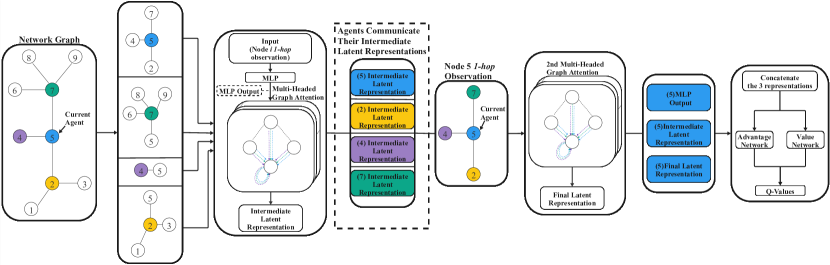
The first architecture we propose is depicted in Figure 1 and consists of an encoder module comprised of three different stages: one Multi Layer Perceptron (MLP) followed by two multi-headed GATs Veličković et al. (2018) with dynamic attention Brody et al. (2022). The final latent representation will comprise the concatenation of each stage output, which is then fed to a dueling network decoding the final representation into the predicted values. After each encoding stage, a activation function is applied.
We now describe the flow from the agent’s observation to the values prediction and we show how it can be integrated into broadcast communication protocols. Agent ’s observation at time is first fed to the MLP encoding stage. This results in a learned representation of the features belonging to agent and its neighbors, denoted respectively and . Following such encoding stage, the output of each of the attention heads of the first GAT is:
| (8) |
where the dynamic attention for the tuple , denoted as , is computed by:
| (9) |
where and are learned. We denote , where is the concatenation operator, as the concatenation of every attention output. Through message passing, each agent receives . These new representations are fed to the second GAT layer, where the computation follows the same logic seen in Equation 8 and 9, producing the embedding .
Finally, the output of each encoding stage is concatenated in a final latent representation :
| (10) |
At this point, is fed to the two separate streams of the dueling network, namely the value network and the advantage network , parameterized by two separate MLPs with parameters and , respectively. Let us denote the parameterization previous to the dueling network, which produced the final latent representation given , as . The predicted values are then obtained as:
| (11) |
We note that the encoding process described above harmoniously integrates with the communication mechanisms present in protocols deployed in the real world, such as OLSR. We envision every node (agent) in the network, feeding its neighborhood structure through the encoding process described above. Subsequently, every agent shares their intermediate representation with their one-hop neighbors, in a similar way to how nodes communicate their MPR sets in OLSR. Once the representations are collected, agents feed them to the second GAT layer, obtaining .
However, embedding the communication process generates a communication overhead of size proportional to , an aspect which might need to be further minimized in bandwidth-constrained networks Suri et al. (2023); Galliera et al. (2023). This observation leads us to our second approach.
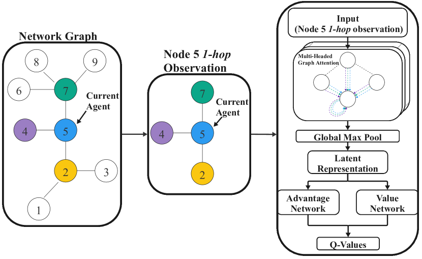
4.2.3 Hyperlocal-DyAN
Intending to generate less communication overhead, we design a second model, named HL-DyAN, which resembles L-DyAN in its form. We replace the three encoding stages with a single GAT layer with dynamic attention. Within agent ’s observation, we apply the GAT encoding process to every node, followed by a activation function. Finally, a global max-pooling layer is applied to summarize the most salient neighborhood characteristics, as shown in Figure 2.
The rationale for this approach is that agents can make informed decisions by processing their one-hop neighborhood dynamics from each neighbor’s perspective, eliminating the need to share their latent representations, as seen in L-DyAN.
In detail, agent ’s observation at time is fed to the GAT layer and, as opposed to L-DyAN, such an operation is repeated for every node within the local observation of agent , producing a set of latent representations comprising and . We then perform global max pooling, obtained through a feature-wise max operation:
| (12) |
Finally, is fed to the dueling network following the same process described in Equation 11.
5 Experiments
In this section, we detail our experimental design to evaluate our two methods against DGN and the MPR heuristic employed in OLSR. Finally, we discuss our results.
| Max Node Degree (Start) | Nodes Speed | Metric | L-DyAN | HL-DyAN | MPR Heuristic | DGN |
| 5 Neighbors | Messages | 28.22 4.52 | 34.81 8.27 | 25.64 7.47 | 3.88 2.94 | |
| Coverage | 93.78% 13.58 | 90.02% 19.93 | 86.24% 22.40 | 24.34% 16.24 | ||
| 5 Neighbors | Messages | 24.05 6.95 | 33.40 8.23 | 8.21 5.85 | 6.69 4.39 | |
| Coverage | 79.34% 21.64 | 83.64% 19.99 | 34.02% 20.81 | 35.77% 21.15 | ||
| 10 Neighbors | Messages | 23.26 5.67 | 33.06 7.43 | 22.95 7.26 | 15.91 2 | |
| Coverage | 88.51% 19.46 | 89.59% 19.65 | 85.73% 23.63 | 24.35% 13.54 | ||
| 10 Neighbors | Messages | 24.31 5.38 | 37.01 5.26 | 8.10 6.14 | 7.03 4.57 | |
| Coverage | 86.33% 16.99 | 91.69% 12.67 | 37.98% 23.55 | 42.74% 24.45 | ||
| 25 Neighbors | Messages | 23.74 5.85 | 34.15 4.72 | 24.93 5.35 | 3.28 2.23 | |
| Coverage | 90.44% 18.80 | 93.84% 9.85 | 92.86% 15.98 | 26.33 16.02 | ||
| 25 Neighbors | Messages | 24.29 5.67 | 36.35 4.64 | 10.03 6.75 | 6.96 4.48 | |
| Coverage | 88.19% 17.62 | 92.23% 11.06 | 46.80% 27.05 | 44.02% 25.50 | ||
| 49 Neighbors | Messages | 22.99 5.85 | 34.34 4.82 | 23.92 6.97 | 3.47 2.36 | |
| Coverage | 89.73% 20.02 | 91.96% 18.04 | 88.93% 20.04 | 27.16% 15 | ||
| 49 Neighbors | Messages | 24.81 4.95 | 36.61 5.78 | 9.39 6.57 | 6.81 4.14 | |
| Coverage | 88.86% 15.34 | 92.42% 13.51 | 43.49% 25.67 | 41.33% 22.61 |
Experimental Setup
We generated 50,000 connected graph topologies for training, each consisting of 50 nodes with a broadcasting range of 20 and no constraints on the number of neighbors. For every learning algorithm, training was conducted five times adopting different random seeds (4, 9, 17, 42, 43) for 1 million agent steps. In each training episode, the environment randomly selected a graph as the initial graph and a node as the source. To mitigate strong mobility pattern biases, a random state generator determined the nodes’ movements, which was seeded anew at the beginning of every episode. The nodes’ speed is defined in terms of per and was set to 6 during training.
Furthermore, we utilized 4 distinct sets of connected starting graph topologies, not seen during training, for testing purposes. These sets comprised 50 nodes per graph with various constraints on the maximum node degree allowed (5, 10, 25, and 49). Our evaluation process involved testing each graph 50 times and selecting a different node as the source in each iteration. To promote reproducibility and ensure the coherence of results, the same random state generator was used to control the nodes’ movements across iterations for the same graph. Additional evaluations were conducted on the impact of the nodes’ velocity setting their speed to , , and .
Our analysis compared L-DyAN and HL-DyAN with the MPR heuristic and DGN. The DGN methodology excluded Temporal Relation Regularization, as it was unnecessary in our setting where agent interaction is temporally bounded by a short local horizon. To ensure a fair evaluation, we maintained consistent hyperparameters across all models, the details of which are presented in Table 4-Appendix A.4.3.
Results
Table 2 shows the results of our experiments in terms of coverage and messages required to achieve it, presenting the means and standard deviations. Our proposed methods, L-DyAN and HL-DyAN, consistently demonstrate higher coverage across different scenarios compared to MPR and DGN. In particular, HL-DyAN achieves the highest coverage with a mean of 90.37%. However, this comes at the cost of a higher number of messages, with HL-DyAN generating an average of 34.85 messages per episode. L-DyAN, while slightly less successful in coverage (87.70%), requires significantly fewer messages (24.32), indicating its suitability in scenarios where message efficiency is prioritized over coverage.
As the nodes’ speed increases, the performance gap between our proposed methods and MPR widens, with L-DyAN and HL-DyAN maintaining superior coverage across all tests with increased speed. This is further supported by additional tests we conducted with the nodes’ speed set to 10, obtaining a coverage of , resp. with resp. messages, by L-DyAN and HL-DyAN. MPR, instead, struggled to reach of coverage. Additionally, in the more dynamic scenarios with speed set to be greater than 1, the maximum node degree negatively influences the performance of all methods, but L-DyAN and HL-DyAN consistently outperform the other algorithms, which fail to reach 50% coverage. This indicates the robustness of L-DyAN and HL-DyAN to dynamic scenarios with less dense neighborhoods.
In more static scenarios where the node speed is set to 1, L-DyAN and MPR reveal to be the more efficient reaching, respectively, 14.84 and 14.54 percent of coverage per message.
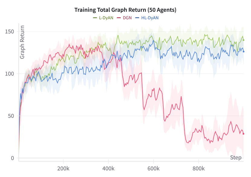
Figure 3 illustrates the training progress of L-DyAN, HL-DyAN, and DGN over multiple cycles using five distinct random seeds. Our proposed methodologies, L-DyAN and HL-DyAN, demonstrated an average of the total graph returns (sum of all the agents returns) of and , respectively. In contrast, the training trajectory of DGN indicates a more brittle learning progress, unable to learn an effective multi-agent strategy for this task.
Discussion
The results underscore the efficiency of L-DyAN and HL-DyAN in learning effective multi-agent strategies balancing message efficiency with coverage consistently across various scenarios. MPR falls short in both slightly and very dynamic and/or sparsely connected environments, with its performance worsening as nodes are faster and their starting neighborhood more sparse. The results also highlight the adaptability of L-DyAN and HL-DyAN in varying network densities and node velocities, making them suitable for a wide range of dynamic network environments. Additionally, the training behavior of the three learning algorithms highlights the strengths of our method in learning multi-agent strategies for networked environments, where the presence of the agents and the structure of their neighborhoods change dynamically.
6 Conclusion and Future Work
In this work, we captured the problem of information dissemination in dynamic broadcast networks in a novel POSG formulation and proposed two MARL methods to solve the task, namely L-DyAN and HL-DyAN. Our experiments showed how these methods outperform in terms of coverage and message efficiency both DGN and a popular heuristic employed in widely adopted broadcast protocols.
Our future research agenda includes investigating more structured group communication tasks, where, for example, coverage is desired only for a subset of nodes or nodes with higher priority. We will also study methods to enable more controlled trade-offs between coverage and forwarded messages, as well as their application in deployed protocols for physical computer networks. Orthogonally, we will investigate the application of our approach to the dissemination of information in other domains, such as social networks and computational social choice.
References
- Ahmed et al. [2022] Ibrahim H. Ahmed, Cillian Brewitt, Ignacio Carlucho, Filippos Christianos, Mhairi Dunion, Elliot Fosong, Samuel Garcin, Shangmin Guo, Balint Gyevnar, Trevor McInroe, Georgios Papoudakis, Arrasy Rahman, Lukas Schäfer, Massimiliano Tamborski, Giuseppe Vecchio, Cheng Wang, and Stefano V. Albrecht. Deep reinforcement learning for multi-agent interaction. AI Commun., 35(4):357–368, 2022.
- Albrecht et al. [2023] Stefano V. Albrecht, Filippos Christianos, and Lukas Schäfer. Multi-Agent Reinforcement Learning: Foundations and Modern Approaches. MIT Press, 2023.
- Brody et al. [2022] Shaked Brody, Uri Alon, and Eran Yahav. How attentive are graph attention networks? In International Conference on Learning Representations (Poster), 2022.
- Buşoniu et al. [2010] Lucian Buşoniu, Robert Babuška, and Bart De Schutter. Multi-agent Reinforcement Learning: An Overview, pages 183–221. Springer Berlin Heidelberg, Berlin, Heidelberg, 2010.
- Das et al. [2019] Abhishek Das, Théophile Gervet, Joshua Romoff, Dhruv Batra, Devi Parikh, Mike Rabbat, and Joelle Pineau. TarMAC: Targeted multi-agent communication. In Kamalika Chaudhuri and Ruslan Salakhutdinov, editors, Proceedings of the 36th International Conference on Machine Learning, volume 97 of Proceedings of Machine Learning Research, pages 1538–1546. PMLR, 09–15 Jun 2019.
- Dearlove and Clausen [2014] Christopher Dearlove and Thomas H. Clausen. Optimized Link State Routing Protocol Version 2 (OLSRv2) and MANET Neighborhood Discovery Protocol (NHDP) Extension TLVs. RFC 7188, April 2014.
- Fey and Lenssen [2019] Matthias Fey and Jan E. Lenssen. Fast graph representation learning with PyTorch Geometric. In ICLR Workshop on Representation Learning on Graphs and Manifolds, 2019.
- Foerster et al. [2016] Jakob N. Foerster, Yannis M. Assael, Nando de Freitas, and Shimon Whiteson. Learning to communicate with deep multi-agent reinforcement learning. In Proceedings of the 30th International Conference on Neural Information Processing Systems, NIPS’16, page 2145–2153, Red Hook, NY, USA, 2016. Curran Associates Inc.
- Galliera et al. [2023] Raffaele Galliera, Mattia Zaccarini, Alessandro Morelli, Roberto Fronteddu, Filippo Poltronieri, Niranjan Suri, and Mauro Tortonesi. Learning to sail dynamic networks: The marlin reinforcement learning framework for congestion control in tactical environments. In MILCOM 2023 - 2023 IEEE Military Communications Conference (MILCOM), pages 424–429, 2023.
- Garey and Johnson [1979] M. R. Garey and David S. Johnson. Computers and Intractability: A Guide to the Theory of NP-Completeness. W. H. Freeman, 1979.
- Guille et al. [2013] Adrien Guille, Hakim Hacid, Cecile Favre, and Djamel A. Zighed. Information diffusion in online social networks: A survey. SIGMOD Rec., 42(2):17–28, jul 2013.
- Hagberg et al. [2008] Aric Hagberg, Pieter J. Swart, and Daniel A. Schult. Exploring network structure, dynamics, and function using networkx. 1 2008.
- Hamilton et al. [2017] William L. Hamilton, Rex Ying, and Jure Leskovec. Inductive representation learning on large graphs. In Proceedings of the 31st International Conference on Neural Information Processing Systems, NIPS’17, page 1025–1035, Red Hook, NY, USA, 2017. Curran Associates Inc.
- Hausknecht and Stone [2015] Matthew J. Hausknecht and Peter Stone. Deep recurrent q-learning for partially observable mdps. In 2015 AAAI Fall Symposia, Arlington, Virginia, USA, November 12-14, 2015, pages 29–37. AAAI Press, 2015.
- Ibrahim et al. [2020] Banar Fareed Ibrahim, Mehmet Toycan, and Hiwa Abdulkarim Mawlood. A comprehensive survey on vanet broadcast protocols. In 2020 International Conference on Computation, Automation and Knowledge Management (ICCAKM), pages 298–302, 2020.
- Jiang and Lu [2018] Jiechuan Jiang and Zongqing Lu. Learning attentional communication for multi-agent cooperation. In Proceedings of the 32nd International Conference on Neural Information Processing Systems, NIPS’18, page 7265–7275, Red Hook, NY, USA, 2018. Curran Associates Inc.
- Jiang et al. [2020] Jiechuan Jiang, Chen Dun, Tiejun Huang, and Zongqing Lu. Graph convolutional reinforcement learning. In International Conference on Learning Representations, 2020.
- Kaviani et al. [2021] Saeed Kaviani, Bo Ryu, Ejaz Ahmed, Kevin A. Larson, Anh Le, Alex Yahja, and Jae H. Kim. Deepcq+: Robust and scalable routing with multi-agent deep reinforcement learning for highly dynamic networks. In 2021 IEEE Military Communications Conference, MILCOM 2021, San Diego, CA, USA, November 29 - Dec. 2, 2021, pages 31–36. IEEE, 2021.
- Kaviani et al. [2023] Saeed Kaviani, Bo Ryu, Ejaz Ahmed, Deokseong Kim, Jae Kim, Carrie Spiker, and Blake Harnden. Deepmpr: Enhancing opportunistic routing in wireless networks through multi-agent deep reinforcement learning, 2023.
- Kipf and Welling [2017] Thomas N. Kipf and Max Welling. Semi-supervised classification with graph convolutional networks. In International Conference on Learning Representations, 2017.
- Ma et al. [2012] Xiaomin Ma, Jinsong Zhang, Xiaoyan Yin, and Kishor S. Trivedi. Design and analysis of a robust broadcast scheme for vanet safety-related services. IEEE Transactions on Vehicular Technology, 61(1):46–61, 2012.
- Macker [2012] J. Macker. Rfc 6621: Simplified multicast forwarding, 2012.
- Peng et al. [2017] Peng Peng, Ying Wen, Yaodong Yang, Quan Yuan, Zhenkun Tang, Haitao Long, and Jun Wang. Multiagent bidirectionally-coordinated nets: Emergence of human-level coordination in learning to play starcraft combat games, 2017.
- Puterman [1994] Martin L. Puterman. Markov Decision Processes: Discrete Stochastic Dynamic Programming. John Wiley & Sons, Inc., USA, 1st edition, 1994.
- Qayyum et al. [2002] A. Qayyum, L. Viennot, and A. Laouiti. Multipoint relaying for flooding broadcast messages in mobile wireless networks. In Proceedings of the 35th Annual Hawaii International Conference on System Sciences, pages 3866–3875, 2002.
- Scarselli et al. [2009] Franco Scarselli, Marco Gori, Ah Chung Tsoi, Markus Hagenbuchner, and Gabriele Monfardini. The graph neural network model. IEEE Transactions on Neural Networks, 20(1):61–80, 2009.
- Schulman et al. [2017] John Schulman, Filip Wolski, Prafulla Dhariwal, Alec Radford, and Oleg Klimov. Proximal policy optimization algorithms, 2017.
- Sukhbaatar et al. [2016] Sainbayar Sukhbaatar, Arthur Szlam, and Rob Fergus. Learning multiagent communication with backpropagation. In Proceedings of the 30th International Conference on Neural Information Processing Systems, NIPS’16, page 2252–2260, Red Hook, NY, USA, 2016. Curran Associates Inc.
- Suri et al. [2022] Niranjan Suri, Maggie Bredy, Lorenzo Campioni, Jan Nilsson, Eelco Cramer, Roberto Fronteddu, and Mauro Tortonesi. Comparing performance of group communications protocols over scb versus routed manet networks. In MILCOM 2022 - 2022 IEEE Military Communications Conference (MILCOM), pages 1011–1017, 2022.
- Suri et al. [2023] Niranjan Suri, Lorenzo Campioni, Edoardo Di Caro, Maggie Breedy, Alessandro Morelli, Roberto Fronteddu, and Mauro Tortonesi. Adaptive information dissemination over tactical edge networks. In 2023 International Conference on Military Communications and Information Systems (ICMCIS), pages 1–7, 2023.
- Sutton and Barto [2018] Richard S. Sutton and Andrew G. Barto. Reinforcement Learning: An Introduction. A Bradford Book, Cambridge, MA, USA, 2018.
- Terry et al. [2021] J Terry, Benjamin Black, Nathaniel Grammel, Mario Jayakumar, Ananth Hari, Ryan Sullivan, Luis S Santos, Clemens Dieffendahl, Caroline Horsch, Rodrigo Perez-Vicente, et al. Pettingzoo: Gym for multi-agent reinforcement learning. Advances in Neural Information Processing Systems, 34:15032–15043, 2021.
- Tonguz et al. [2007] Ozan Tonguz, Nawapom Wisitpongphan, Fan Bai, Priyantha Mudalige, and Varsha Sadekar. Broadcasting in vanet. In 2007 Mobile Networking for Vehicular Environments, pages 7–12, 2007.
- Veličković et al. [2018] Petar Veličković, Guillem Cucurull, Arantxa Casanova, Adriana Romero, Pietro Liò, and Yoshua Bengio. Graph attention networks. In International Conference on Learning Representations, 2018.
- Wang et al. [2016] Ziyu Wang, Tom Schaul, Matteo Hessel, Hado Van Hasselt, Marc Lanctot, and Nando De Freitas. Dueling network architectures for deep reinforcement learning. In Proceedings of the 33rd International Conference on International Conference on Machine Learning - Volume 48, ICML’16, page 1995–2003. JMLR.org, 2016.
- Weng et al. [2022] Jiayi Weng, Huayu Chen, Dong Yan, Kaichao You, Alexis Duburcq, Minghao Zhang, Yi Su, Hang Su, and Jun Zhu. Tianshou: A highly modularized deep reinforcement learning library. Journal of Machine Learning Research, 23(267):1–6, 2022.
- Yahja et al. [2022] Alex Yahja, Saeed Kaviani, Bo Ryu, Jae H. Kim, and Kevin A. Larson. Deepadmr: A deep learning based anomaly detection for MANET routing. In IEEE Military Communications Conference, MILCOM 2022, Rockville, MD, USA, November 28 - December 2, 2022, pages 412–417. IEEE, 2022.
- Ye and Zhou [2021] Zipeng Ye and Qingrui Zhou. Performance evaluation indicators of space dynamic networks under broadcast mechanism. Space: Science & Technology, 2021, 2021.
Appendix A Technical Appendix
A.1 Pseudo-code of the MPR Selection algorithm
is defined as the number of symmetric neighbors of node , excluding all the members of and excluding the node performing the computation.
A poorly covered node is a node in which is covered by less than MPR_COVERAGE nodes in .
Note that in our implementation every node has willingness set to WILL_ALWAYS and MPR_COVERAGE is set to 1 to ensure that the MPR heuristic’s overhead is kept to the minimum.
| Max Node Degree (Start) | Nodes Speed | Metric | L-DyAN | HL-DyAN | MPR Heuristic | DGN |
| 5 Neighbors | Messages | 28.22 4.52 | 34.81 8.27 | 25.64 7.47 | 3.88 2.94 | |
| Coverage | 93.78% 13.58 | 90.02% 19.93 | 86.24% 22.40 | 24.34% 16.24 | ||
| 5 Neighbors | Messages | 26.21 5.85 | 34.55 7.35 | 14.33 8.42 | 5.21 3.80 | |
| Coverage | 87.78% 18.53 | 88.65% 17.74 | 54.53% 28.27 | 30.49% 19.33 | ||
| 5 Neighbors | Messages | 24.05 6.95 | 33.40 8.23 | 8.21 5.85 | 6.69 4.39 | |
| Coverage | 79.34% 21.64 | 83.64% 19.99 | 34.02% 20.81 | 35.77% 21.15 | ||
| 5 Neighbors | Messages | 22.10 7.17 | 32.50 7.97 | 4.49 3.18 | 9.34 5.02 | |
| Coverage | 71.96% 21.47 | 79.78% 19.75 | 21.54% 12.63 | 45.32% 22.64 | ||
| 10 Neighbors | Messages | 23.26 5.67 | 33.06 7.43 | 22.95 7.26 | 15.91 2 | |
| Coverage | 88.51% 19.46 | 89.59% 19.65 | 85.73% 23.63 | 24.35% 13.54 | ||
| 10 Neighbors | Messages | 24.34 5.88 | 35.97 5.98 | 16.10 8.58 | 4.07 3.04 | |
| Coverage | 88.73% 18.83 | 93.30% 14.39 | 65.4% 30.46 | 29.36% 19.06 | ||
| 10 Neighbors | Messages | 24.31 5.38 | 37.01 5.26 | 8.10 6.14 | 7.03 4.57 | |
| Coverage | 86.33% 16.99 | 91.69% 12.67 | 37.98% 23.55 | 42.74% 24.45 | ||
| 10 Neighbors | Messages | 24.66 5.38 | 35.98 6.11 | 5.05 3.69 | 9.72 4.91 | |
| Coverage | 82.32% 16.70 | 88.06% 14.62 | 26.61% 15.36 | 52.15% 23.58 | ||
| 25 Neighbors | Messages | 23.74 5.85 | 34.15 4.72 | 24.93 5.35 | 3.28 2.23 | |
| Coverage | 90.44% 18.80 | 93.84% 9.85 | 92.86% 15.98 | 26.33 16.02 | ||
| 25 Neighbors | Messages | 24.33 5.11 | 36.05 4.57 | 17.73 7.59 | 4.25 3.08 | |
| Coverage | 90.81% 15.26 | 93.49% 10.38 | 72.92% 27.48 | 31.04% 19.16 | ||
| 25 Neighbors | Messages | 24.29 5.67 | 36.35 4.64 | 10.03 6.75 | 6.96 4.48 | |
| Coverage | 88.19% 17.62 | 92.23% 11.06 | 46.80% 27.05 | 44.02% 25.50 | ||
| 25 Neighbors | Messages | 24.46 5.36 | 35.78 5.07 | 5.75 4.41 | 9.50 4.94 | |
| Coverage | 84.79% 15.76 | 89.87% 11.98 | 30.32% 19.28 | 51.89% 24.83 | ||
| 49 Neighbors | Messages | 22.99 5.85 | 34.34 4.82 | 23.92 6.97 | 3.47 2.36 | |
| Coverage | 89.73% 20.02 | 91.96% 18.04 | 88.93% 20.04 | 27.16% 15 | ||
| 49 Neighbors | Messages | 23.9 5.43 | 35.8 6.13 | 16.45 8.02 | 4.76 3.27 | |
| Coverage | 90.05% 18.72 | 93.02% 15.04 | 67.91% 28.87 | 33.38% 19.25 | ||
| 49 Neighbors | Messages | 24.81 4.95 | 36.61 5.78 | 9.39 6.57 | 6.81 4.14 | |
| Coverage | 88.86% 15.34 | 92.42% 13.51 | 43.49% 25.67 | 41.33% 22.61 | ||
| 49 Neighbors | Messages | 23.88 5.52 | 35.55 5.16 | 4.81 3.63 | 9.81 4.81 | |
| Coverage | 82.35% 17.32 | 88.83% 12.24 | 26.68% 16.69 | 52.69% 23.77 | ||
| Total Mean Std | Messages | 24.35 5.69 | 35.12 6.23 | 13.62 6.47 | 6.92 3.88 | |
| Total Mean Std | Coverage | 86.50% 18.01 | 90.02% 15.46 | 55.12% 22.99 | 37.02% 20.71 | |
| Every experiment is performed over 500 different starting graphs. Results report mean and standard deviation. | ||||||
A.2 Extended Results
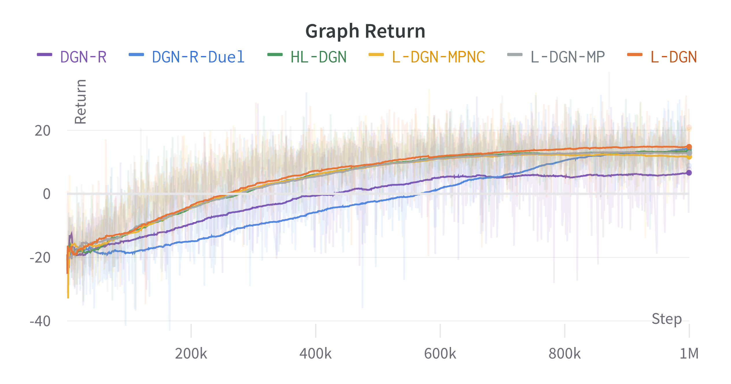
A.3 Ablation Study
We investigate different ablations of L-DyAN, whose architectures lay between L-DyAN and HL-DyAN, and DGN. Their performance is measured in terms of the summation of the returns achieved by each agent that has participated in the dissemination task, named “graph return” (Figure 4). Given that our environment is highly dynamic in terms of the entities contributing to the dissemination task at each timestep, such a metric allows us to understand if the local rewards assigned to each agent correlate with a desired overall collaboration across the entire graph, measured in terms of summations of the rewards achieved. We trained these policies on static scenarios with graphs of 20 nodes.
L-DyAN-Duel. The implementation of this method lies between L-DyAN and DGN. Starting from the latter, we added the dueling network instead of a single MLP stream as the action decoder. Figure 4 shows the positive impact of the dueling network in the final strategy, which significantly outperforms L-DyAN after 600K steps. From such a learning trajectory, we can also deduce the impact of another main component of our L-DyAN, the n-step return estimation proportional to the local horizon (see Cooperative Dynamic Neighborhoods). With the addition of such n-step returns, we obtain our L-DyAN architecture, and we can notice how such a component helps the learned strategy to converge earlier and less abruptly.
L-DyAN-MP. This method removes the second GAT layer of L-DyAN and replaces it with the global max pool operator (later adopted by HL-DyAN). The concatenation of the output of every encoding stage is still present here. We can notice a slight drop in performance when compared to L-DyAN.
L-DyAN-MPNC. This method removes both the second GAT layer of L-DyAN, as well as the concatenation of the output of every encoding stage. We notice a decrease in performance when compared to L-DyAN. It can also be seen that HL-DyAN can be derived from L-DyAN-MPNC after the ablation of the MLP encoding stage and that HL-DyAN does not suffer from such performance reduction.
In summary, these ablation studies centered around L-DyAN allow us to both understand the strengths of this approach when compared to DGN, as well as motivate the design of the HL-DyAN architecture, which exhibits a simplified structure, less communication overhead, and only slightly underperforms in terms of graph return during training.
A.4 Additional Reproducibility Details and Instructions
A.4.1 Implementation Details
Our framework, which is written in Python and based on PyTorch, implements a customized extension of Tianshou Weng et al. [2022]. The MARL environment is defined following the PettingZoo Terry et al. [2021] API. The GAT, transformer-like dot product attention layer, and global max pooling follow the implementation provided by PyTorch Geometric Fey and Lenssen [2019]. Training and testing graphs were generated with the aid of the NetworkX library Hagberg et al. [2008].
A.4.2 Hardware Involved
Our policies were trained using 40 parallel environments on a workstation running Ubuntu 22.04 LTS, CUDA Toolkit v11.7, and equipped with an Intel i9-13900F CPU, 32GB DDR4 RAM, and an NVIDIA GeForce RTX 4090 GPU.
A.4.3 Hyperparameters
| Hyperparameter | Value | |
| Training | ||
| Training steps | ||
| Learning rate | ||
| Buffer size | ||
| Gamma | ||
| Batch size | 32 | |
| Exploration Decay | Exponential | |
| Local Horizon | ||
| N-Step Estimation | ||
| Training Frequency | 1 per 160 Agent steps | |
| Gradient Steps | ||
| Parallel Training Envs | 40 | |
| Experience Replay | Uniform | |
| Seed | 4, 9, 17, 42, 43 | |
| Policy Params. | ||
| MLP Hidden Size | 32 | |
| GAT Attention Heads | ||
| GAT Hidden Size | 32 (each head) | |
| A-Network Hidden Sizes | [128, 128] | |
| V-Network Hidden Sizes | [128, 128] |
A.4.4 Instructions
To ease testing and reproducibility, our framework comes with a Docker Image comprising all the requirements that the reader can quickly build, allowing them to run the application in a containerized environment following the instructions listed below.
-
1)
From the root project folder run the following command to build the image:
docker build -t marl_mpr .
-
1b)
If the host machine does not have any GPU or if it is an Apple Mac device (including ones employing Apple MX SoC) please use:
docker build -t marl_mpr \
-f Dockefile.cpu . -
2)
Command example to run the container:
docker run --ipc=host --gpus all \
-v ${PWD}:/home/devuser/dev:Z \-it --rm marl_mprPlease note that
--gpus allis optional and it should be omitted in case the hosting machine is not equipped with a GPU. Alternatively, the reader can also install the requirements needed in a dedicated Python () virtual environment by runningpip install -r requirements.txt
-
3)
Visualization (Optional). A visualization aid is provided to watch the agents in action on the testing graphs. If the Docker Image is used, the following two arguments should be added when running the container in order to render the figure:
-e DISPLAY=unix\$DISPLAYand-v /tmp/.X11-unix:/tmp/.X11-unix.333Please note that these arguments are valid only for machines running a Unix OS. Machines running MacOS might require installing a display server like XQuartz. The entire command to run the container while enabling visualization would be:docker run --ipc=host --gpus all \
-e DISPLAY=unix$DISPLAY \-v /tmp/.X11-unix:/tmp/.X11-unix \-v ${PWD}:/home/devuser/dev:Z \-it --rm marl_mpr
A.4.5 Training models
Trained models will be saved in the
log/algorithm_name/weights folder as model_name_last.pth. Before the training process begins, the user will be asked if they want to log training data using the Weight and Biases (WANDB) logging tool.
-
•
DGN
python train_dgn.py \--model-name DGN -
•
L-DyAN
python train_l_dyan.py \--model-name L-DyAN \ -
•
HL-DyAN
python train_hl_dyan.py \--model-name HL-DyAN
Seeding
Results reported are based on 5 different random seeds . By default, our scripts set the seed to 9. The reader can easily change such value using the argument --seed X, where X is the chosen seed. This seeding value is carefully set for np_random.seed(X), toch.manual_seed(X), train_envs.seed(X), and
test_envs.seed(X). Other parameters can be changed from their default and they can be consulted via python train_dgn.py --help.
A.4.6 Testing models
All three of our trained models, DGN, L-DyAN, and HL-DyAN, are found in their respective subfolders of the /log folder and results can be reproduced with the following command:
-
•
DGN
python train_dgn.py --watch \--model-name DGN.pth -
•
L-DyAN
python train_l_dyan.py --watch \--model-name L-DyAN.pth -
•
HL-DyAN
python train_hl_dyan.py --watch \--model-name HL-DyAN.pth -
•
MPR Heuristic. In order to test MPR heuristic results add the boolean argument
--mpr-policy. For example:python train_hl_dyan.py --watch \--model-name HL-DyAN.pth \ --mpr-policy
A.4.7 Topologies Dataset
As mentioned in the Experiments Training and testing sets contain, respectively, 50K and 130 graphs. The sole dataset takes up to 140MB compressed in a ZIP file with maximum compression level, for such a reason, and for reviewing purposes, we upload (along with the code) a reduced training set of topologies with 10000 graphs. The testing set is left unchanged. All the topologies can be found in the /graph_topologies folder.