Explicit lump and line rogue wave solutions to a modified Hietarinta equation

Abstract

Lump solutions are spatially rationally localized solutions which usually arise as solutions to higher dimensional nonlinear partial differential equations often possessing Hirota bilinear forms. Under some parameter constraint, these solutions may lead to rogue wave solutions. In this article, we study lump and rogue wave solutions of a new nonlinear non-evolutionary equation in 2+1 dimensions with the aid of a computer algebra system. We present illustrative examples and analyze the dynamical behavior of the solutions using graphical representations.

Key words: Lump solutions, Rogue waves, Hirota bilinear form, Hietarinta equation
PACS codes: 02.30.Ik, 04.20.Fy, 05.45.Yv
MSC codes: 35C08; 35Q51

1 Introduction

Lump solutions, which are analytic and spatially localized rational solutions to higher dimensional nonlinear partial differential equations, have been an active research area in mathematical physics over the last few years. They were first found by Manakov and Zakharov [1] for the KP equation by taking long wave limits of $N$-solitons [1, 2, 3, 4], but have recently been found in several integrable and nonintegrable equations (see e.g., [2, 5, 6, 7, 8, 9, 10]). Apart from taking long wave limits, one can also derive lump solutions via Hirota’s method [11, 12] or the singular manifold method [13, 14, 15]. Research has shown that lump solutions have many applications in nonlinear dynamics [6]. They provide appropriate prototypes to model rogue wave dynamics in oceanography [16] and nonlinear optics [17].

Recently, lump solutions have been found to generate a type of rogue wave solutions known as line rogue waves, which may arise under some parameter constraint [18]. Line rogue waves [18] usually emerge from a constant background with line profiles which eventually decay into the constant background. Rogue waves have also been of considerable interest in recent years due to emerging applications in other contexts such as nonlinear optics [17] and the atmosphere [19]. For rogue waves in other physical contexts, see [20]. The most universal mathematical model for the study of rogue waves is the one-dimensional focusing Nonlinear Schrödinger equation [21, 22]. However, other integrable models, notably, the Kadomtsev-Petviashvili equation [5, 23], the Hirota-Satsuma-Ito equation [8, 24] and the B-type KP equation [25, 26, 27] have also been used to study rogue waves.

In this article, we study lump and line rogue wave solutions of a novel (2+1)-dimensional equation which is an extension of the so-called Hietarinta equation [12]. We will employ Hirota’s method [11] which is perhaps the most effective tool for finding exact solutions, particularly soliton solutions (see e.g., [28, 29]), to nonlinear equations that possess Hirota bilinear forms. To use this method to find lump solutions, one constructs positive quadratic function solutions to a bilinear equation and uses logarithmic transformations to obtain the desired solutions (see e.g., [5, 30, 31, 32, 33]). First, we introduce a (2+1)-dimensional equation as a modification of the (1+1)-dimensional Hietarinta equation. We further formulate its Hirota bilinear form and construct positive quadratic solutions to this bilinear equation. Consequently, we construct lump and line rogue waves to the newly introduced equation. The paper concludes with illustrative examples and some concluding remarks.

2 A modified Hietarinta equation

The bilinear Hietarinta equation [12] is given by,

$$(D_{x}^{4}-D_{x}D_{t}^{3}+\alpha D_{x}^{2}+\beta D_{x}D_{t}+\gamma D_{t}^{2})f\cdot f=0,$$ (1)

where $\alpha,\beta,\gamma$ are constants and $D_{x},D_{t}$ are Hirota derivatives [11]. This equation is in (1+1)-dimensions and is integrable in the sense that it has at least four soliton solutions and also passes the Painlevé test [12, 34]. It is important to point out that there has been no report so far on the existence of rationally localized wave solutions to the Hietarinta equation. Recently, some (2+1)-dimensional extensions of the above equation have been introduced and shown to possess rationally localized wave solutions. For example, Batwa and Ma [35] introduced the bilinear modified Hietarinta equation

$$(\alpha_{1}D_{x}^{4}+\alpha_{2}D_{x}D_{t}^{3}+\gamma_{1}D_{y}D_{t}+\gamma_{2}D_{x}^{2}+\gamma_{3}D_{x}D_{t}+\gamma_{4}D_{x}D_{y}+\gamma_{5}D_{y}^{2})f\cdot f=0,$$ (2)

and found lump solutions to the associated (2+1)-dimensional nonlinear equation. Manukure and Zhou [36] also introduced the modified Hietarinta bilinear equation

$$(D_{x}^{4}+D_{x}D_{t}^{3}+\alpha D_{x}^{2}+\beta D_{x}D_{t}+\gamma D_{t}^{2}-D_{t}D_{y})f\cdot f=0,$$ (3)

and derived lump and line rogue waves to the associated nonlinear equation. Here, we introduce yet another extension of the bilinear Hietarinta equation as follows,

$$B(f)=(D_{x}^{4}+D_{x}D_{t}^{3}+\alpha D_{x}^{2}+\beta D_{x}D_{t}+\gamma D_{t}^{2}-D_{x}D_{y})f\cdot f=0.$$ (4)

Under the transformation,

$$u=2(\text{ln}f)_{x},\qquad v=2\text{ln}f,$$ (5)

the corresponding (2+1)-nonlinear equation is found to be

$$P(u)=6u_{x}u_{xx}+u_{xxxx}+3u_{t}u_{tt}+3u_{tx}v_{tt}+u_{xttt}+\alpha u_{xx}+\beta u_{tx}+\gamma u_{tt}-u_{xy}=0,$$ (6)

where $v_{x}=u$, and $\alpha,\beta,$ and $\gamma$ are arbitrary constants. The direct connection between (4) and (6) is given by the equation

$$P(u)=\left(\frac{B(u)}{f}\right)_{x}.$$ (7)

To construct locally rationalized wave solutions, we use the method introduced in [31]. Thus, we find positive quadratic function solutions in the form

$$\begin{cases}f&=g^{2}+h^{2}+a_{9},\\ g&=a_{1}x+a_{2}y+a_{3}t+a_{4},\\ h&=a_{5}x+a_{6}y+a_{7}t+a_{8}.\\ \end{cases}$$ (8)

where $a_{i},1\leq i\leq 9$ are real and $a_{9}>0$. If we assume that $g$ and $h$ are linearly dependent, then $f$ can be reduced to

$$f=\delta_{1}(g+\delta_{2})^{2}+\delta_{3}$$ (9)

where $\delta_{1},\delta_{2},\delta_{3}$ are real and $\delta_{1},\leavevmode\nobreak\ \delta_{3}>0$. It then follows that

$$u=2(\ln f)_{x}=\frac{4a_{1}\delta_{1}(g+\delta_{2})}{f}.$$ (10)

The above solution is degenerate:

$$\lim_{t\to\infty}u\neq 0,$$ (11)

and for $t$ fixed,

$$\lim_{x^{2}+y^{2}\to\infty}u\neq 0.$$ (12)

When $g$ and $h$ are linearly independent, we will obtain lump solutions and line rogue waves under a certain parameter constraint.

3 Lump solutions

Now, let us assume that $g$ and $h$ are linearly independent and the matrix

$$\left(\begin{array}[]{ccc}a_{1}&a_{2}\\ a_{5}&a_{6}\end{array}\right)$$ (13)

is of full rank. This means that the determinant of this matrix is nonzero, i.e.,

$$\Delta:=a_{1}a_{6}-a_{2}a_{5}\neq 0.$$ (14)

Substituting $f$ in (8) into (4), we obtain the following solution set:

$$\begin{cases}&a_{2}=\dfrac{\alpha a_{1}^{3}+\beta a_{1}^{2}a_{3}+(\alpha a_{5}^{2}+\gamma a_{3}^{2}-\gamma a_{7}^{2})a_{1}+a_{3}a_{5}(\beta a_{5}+2\gamma a_{7})}{a_{1}^{2}+a_{5}^{2}},\\ &a_{6}=\dfrac{\alpha a_{5}^{3}+\beta a_{5}^{2}a_{7}+(\alpha a_{1}^{2}-\gamma a_{3}^{2}+\gamma a_{7}^{2})a_{5}+a_{1}a_{7}(\beta a_{1}+2\gamma a_{3})}{a_{1}^{2}+a_{5}^{2}},\\ &a_{9}=-\dfrac{3(a_{1}^{4}+2a_{1}^{2}a_{5}^{2}+a_{3}^{3}a_{1}+a_{3}a_{7}^{2}a_{1}+a_{5}a_{3}^{2}a_{7}+a_{5}^{4}+a_{5}a_{7}^{3})(a_{1}^{2}+a_{5}^{2})}{\gamma(a_{1}a_{7}-a_{3}a_{5})^{2}},\\ \end{cases}$$ (15)

with the $a_{i}$’s as free parameters. To ensure the analyticity of the functions in (5), we impose the conditions

$$a_{9}>0,\leavevmode\nobreak\ \leavevmode\nobreak\ \gamma\neq 0,\leavevmode\nobreak\ \leavevmode\nobreak\ a_{1}a_{7}-a_{3}a_{5}\neq 0.$$ (16)

Note that this condition is sufficient for condition (14) since

$$a_{1}a_{6}-a_{2}a_{5}=\frac{(a_{1}a_{7}-a_{3}a_{5})(\beta a_{1}^{2}+\beta a_{5}^{2}+2\gamma a_{1}a_{3}+2\gamma a_{5}a_{7})}{a_{1}^{2}+a_{5}^{2}}.$$ (17)

Thus, positive quadratic function solutions to the bilinear modified Hietarinta equation (4) take the form:

$$\begin{split}f=&(a_{1}x+\frac{\alpha a_{1}^{3}+\beta a_{1}^{2}a_{3}+(\alpha a_{5}^{2}+\gamma a_{3}^{2}-\gamma a_{7}^{2})a_{1}+a_{3}a_{5}(\beta a_{5}+2\gamma a_{7})}{a_{1}^{2}+a_{5}^{2}}y+a_{3}t+a_{4})^{2}\\ &+(a_{5}x+\frac{\alpha a_{5}^{3}+\beta a_{5}^{2}a_{7}+(\alpha a_{1}^{2}-\gamma a_{3}^{2}+\gamma a_{7}^{2})a_{5}+a_{1}a_{7}(\beta a_{1}+2\gamma a_{3})}{a_{1}^{2}+a_{5}^{2}}y+a_{7}t+a_{8})^{2}\\ &-\frac{3(a_{1}^{4}+2a_{1}^{2}a_{5}^{2}+a_{3}^{3}a_{1}+a_{3}a_{7}^{2}a_{1}+a_{5}a_{3}^{2}a_{7}+a_{5}^{4}+a_{5}a_{7}^{3})(a_{1}^{2}+a_{5}^{2})}{\gamma(a_{1}a_{7}-a_{3}a_{5})^{2}},\end{split}$$ (18)

which consequently yield the following solution to the modified Hietarinta equation (6),

$$u=\frac{4a_{5}h+4a_{1}g}{f},$$ (19)

under the transformation (5), with $g$ and $h$ given by,

$$\begin{cases}g&=a_{1}x+\dfrac{\alpha a_{1}^{3}+\beta a_{1}^{2}a_{3}+(\alpha a_{5}^{2}+\gamma a_{3}^{2}-\gamma a_{7}^{2})a_{1}+a_{3}a_{5}(\beta a_{5}+2\gamma a_{7})}{a_{1}^{2}+a_{5}^{2}}y+a_{3}t+a_{4},\\ h&=a_{5}x+\dfrac{\alpha a_{5}^{3}+\beta a_{5}^{2}a_{7}+(\alpha a_{1}^{2}-\gamma a_{3}^{2}+\gamma a_{7}^{2})a_{5}+a_{1}a_{7}(\beta a_{1}+2\gamma a_{3})}{a_{1}^{2}+a_{5}^{2}}y+a_{7}t+a_{8}.\end{cases}$$ (20)

The solution (19) satisfies the condition

$$\lim\limits_{x^{2}+y^{2}\to\infty}u(x,y,t)=0$$ (21)

for any fixed $t$ and is therefore a lump solution to equation (6).

4 Rogue waves

Rogue waves are large oceanic waves which are localized in both time and space [37, 38]. In this section, we find rogue wave solutions to the modified Hietarinta equation (6) by requiring the matrix (13) to be rank deficient. This requirement imposes a constraint on some of the parameters in (17) which consequently yields line rogue waves. Line rogue waves are known to emerge from a constant background and eventually disappear into the same background.

Now, suppose again that $g$ and $h$ are linearly independent and

$$\mathrm{rank}\left(\begin{array}[]{ccc}a_{1}&a_{2}\\ a_{5}&a_{6}\end{array}\right)<2.$$ (22)

Let $\eta(x,y)=a_{1}x+a_{2}y$. Then, we have

$$g=\eta+a_{3}t+a_{4},\quad h=\delta\eta+a_{7}t+a_{8},$$

for some $\delta\in\mathbb{R}$. It follows that $f$ can be written in the form

$$f=(\delta_{1}\eta+\delta_{2}t+\delta_{3})^{2}+(\delta_{4}t+\delta_{5})^{2}+\delta_{6},$$

where $\delta_{1},\delta_{2},\cdots,\delta_{6}$ are real constants and $\delta_{1}\neq 0,\delta_{4}\neq 0,\delta_{6}>0.$

From the rank condition (22), we have

$$a_{1}a_{6}-a_{2}a_{5}=\frac{(a_{1}a_{7}-a_{3}a_{5})(\beta a_{1}^{2}+\beta a_{5}^{2}+2\gamma a_{1}a_{3}+2\gamma a_{5}a_{7})}{a_{1}^{2}+a_{5}^{2}}=0,$$

which gives rise to the constraint,

$$\beta a_{1}^{2}+\beta a_{5}^{2}+2\gamma a_{1}a_{3}+2\gamma a_{5}a_{7}=0$$ (23)

as a result of condition (16). According to (16), at least one of the constants, $a_{1},\leavevmode\nobreak\ a_{5}$ is nonzero. If we assume that $a_{5}\neq 0$, we can rewrite the above condition (23) as,

$$a_{7}=-\frac{\beta a_{1}^{2}+\beta a_{5}^{2}+2\gamma a_{1}a_{3}}{2\gamma a_{5}},$$ (24)

for $\gamma\neq 0$. Under this condition (24) and condition (16), the solutions in (19) yield a class of solutions that satisfy

$$\lim\limits_{|t|\to\infty}u(x,y,t)=0$$ (25)

for $(x,y)\in\mathbb{R}^{2}$ uniformly. This shows that the resulting solutions are localized in time.

5 Illustrative examples

To depict the dynamical behavior of the localized wave solutions, we choose certain specific values for the parameters.

5.1 Lump solutions

Choosing the parameters,

$$\alpha=1,\beta=-1,\gamma=1,a_{1}=-1,a_{3}=2,a_{4}=-2,a_{5}=1,a_{7}=-3,a_{8}=3,$$

we obtain the nonlinear equation

$$6u_{x}u_{xx}+u_{xxxx}+3u_{t}u_{tt}+3u_{tx}v_{tt}+u_{xttt}+u_{xx}-u_{tx}+u_{tt}-u_{xy}=0,$$ (26)

with corresponding bilinear equation

$$(D_{x}^{4}+D_{x}D_{t}^{3}+D_{x}^{2}-D_{x}D_{t}+D_{t}^{2}-D_{x}D_{y})f\cdot f=0.$$ (27)

The quadratic function solutions to the above bilinear equation is given by

$$f=\left(2t-x-\frac{13}{2}y-2\right)^{2}+\left(-3t+x+\frac{25}{2}y+3\right)^{2}+366,$$ (28)

and the corresponding lump solutions to the nonlinear equation (26) is

$$u=-\frac{8(5t-2x-19y-5)}{26t^{2}-20tx-202ty+4x^{2}+76xy+397y^{2}-52t+20x+202y+758}.$$ (29)

If we choose the the values $t=-20,\leavevmode\nobreak\ 0$ and $20$, we get the particular solutions

$$u=\frac{8(105+2x+19y)}{4x^{2}+76xy+397y^{2}+420x+4242y+12198},$$ (30)

$$u=\frac{8(5+2x+19y)}{4x^{2}+76xy+397y^{2}+20x+202y+758},$$ (31)

and

$$u=\frac{8(-95+2x+19y)}{4x^{2}+76xy+397y^{2}-380x-3838y+10118},$$ (32)

respectively, with 3D and contour plots shown below.

One can easily verify that the above solutions $u$ decays in all spacial directions, ie., they satisfy the condition (21).

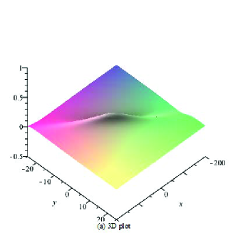
(a)

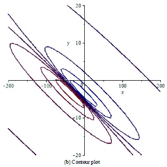
(b)

Fig. 1: Wave profile of solution 30

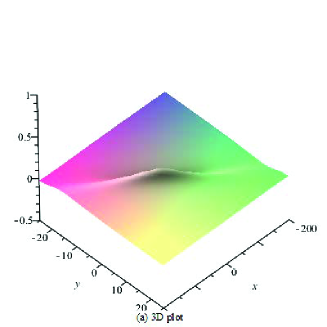
(a)

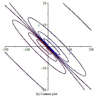
(b)

Fig. 2: Wave profile of solution 31

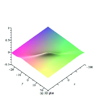
(a)

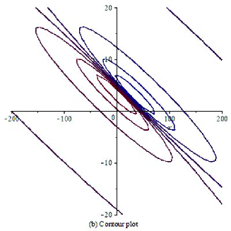
(b)

Fig. 3: Wave profile of solution 32

The amplitude of the wave function (29) is $\displaystyle\frac{2}{\sqrt{283}}$ which is the height of the wave for all values of $t$. Thus, the lump solutions propagate with a constant amplitude at all times.

5.2 Line rogue waves

For line rogue waves, we must choose parameters that satisfy not only condition (16), but also condition (23). To this end, we choose

$$\alpha=1,\beta=1,\gamma=-1,a_{1}=1,a_{3}=2,a_{4}=0,a_{5}=-1,a_{7}=1,a_{8}=3=0.$$

Consequently, we obtain the nonlinear equation

$$6u_{x}u_{xx}+u_{xxxx}+3u_{t}u_{tt}+3u_{tx}v_{tt}+u_{xttt}+u_{xx}+u_{tx}-u_{tt}-u_{xy}=0,$$ (33)

with corresponding bilinear equation

$$(D_{x}^{4}+D_{x}D_{t}^{3}+D_{x}^{2}+D_{x}D_{t}+-D_{t}^{2}-D_{x}D_{y})f\cdot f=0.$$ (34)

The positive quadratic function solution to the above bilinear equation is given by

$$f=\left(2t+x+\frac{7}{2}y\right)^{2}+\left(t-x-\frac{7}{2}y\right)^{2}+6,$$ (35)

and the corresponding lump solution to the nonlinear equation (33) is

$$u=\frac{8(t+2x+7y)}{10t^{2}+4tx+14ty+4x^{2}+28xy+49y^{2}+12}.$$ (36)

If we let $t=-10,-4,-2,0,2,4$ and $10$, we obtain the particular solutions,

$$u=\frac{8(-10+2x+7y)}{4x^{2}+28xy+49y^{2}-40x-140y+1012},$$ (37)

$$u=\frac{8(-4+2x+7y)}{4x^{2}+28xy+49y^{2}-16x-56y+172},$$ (38)

$$u=\frac{8(-2+2x+7y)}{4x^{2}+28xy+49y^{2}-8x-28y+52},$$ (39)

$$u=\frac{8(2x+7y)}{4x^{2}+28xy+49y^{2}+12},$$ (40)

$$u=\frac{8(2+2x+7y)}{4x^{2}+28xy+49y^{2}+8x+28y+52},$$ (41)

$$u=\frac{8(4+2x+7y)}{4x^{2}+28xy+49y^{2}+16x+56y+172},$$ (42)

and

$$u=\frac{8(10+2x+7y)}{4x^{2}+28xy+49y^{2}+40x+140y+1012},$$ (43)

respectively. The 3D plot and contour plots for these solutions are shown below.

(a)

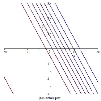
(b)

Fig. 4:
Wave profile of solution 37

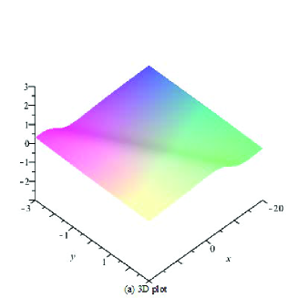
(a)

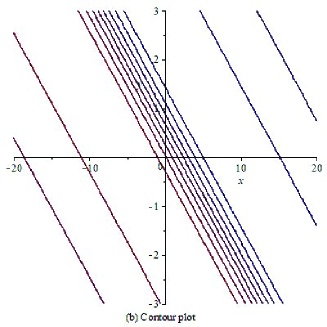
(b)

Fig. 5:
Wave profile of solution 38

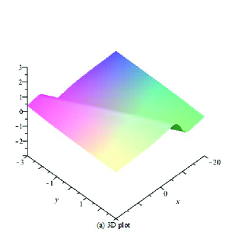
(a)

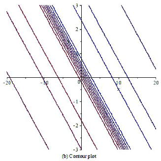
(b)

Fig. 6:
Wave profile of solution 39

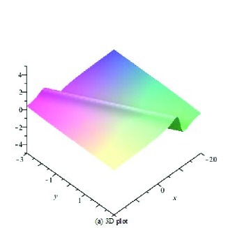
(a)

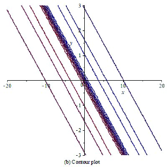
(b)

Fig. 7:
Wave profile of solution 40

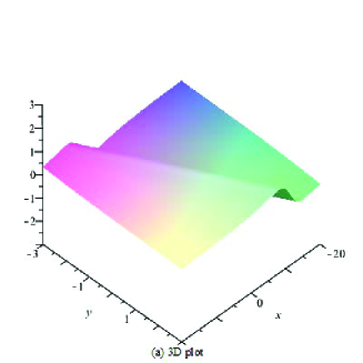
(a)

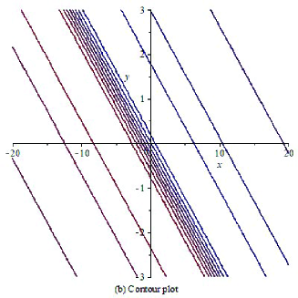
(b)

Fig. 8:
Wave profile of solution 41

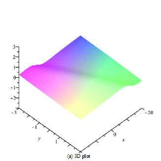
(a)

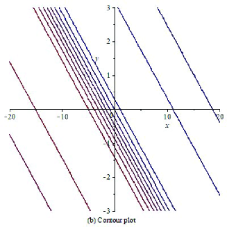
(b)

Fig. 9: Wave profile of solution 42

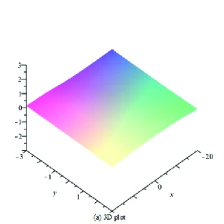
(a)

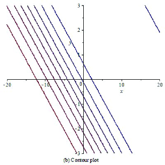
(b)

Fig. 10: Wave profile of solution 43

The solution $u$ in (36) satisfies condition (25) as well as

$$\lim_{x^{2}+y^{2}+t^{2}\to\infty}u(t,x,y)=0,$$ (44)

unless $2x+7y=\epsilon$, for any $\epsilon\in\mathbb{R}$. The maximum of this solution (36) is $\displaystyle\frac{2}{\sqrt{3}}$ which occurs when $t=0$. This means the solution rises from the constant background, peaks when $t=0$ (see Fig. 7) and eventually decays into the constant background.

6 Concluding Remarks

By means of the Hirota bilinear method, we have constructed lump and rogue wave solutions to a so-called modified Hietarinta equation formulated from the (1+1)-dimensional Hietarinta equation. The lump solutions arise from quadratic function solutions of the associated bilinear equation whereas the rogue waves arise from a certain parameter constraint. The lump solutions have been shown to be spatially localized while the line rogue waves are both spatially and temporally localized. More specifically, the lump solutions are localized in all spatial directions and propagate with a constant amplitude of $2/\sqrt{283}$ for all values of $t$ on a constant background. The line rogue wave on the other hand emerges with a line profile from a constant background and rises in amplitude or height to a maximum of $2/\sqrt{3}$ after which it begins to decay and finally disappears into the constant background.

As indicated earlier, a few other modifications of the Hietarinta equation [12] have been presented in literature [35, 36]. The modified Hietarinta equation presented by Batwa and Ma in [35] possesses only lump solutions. In the case of Manukure and Zhou [36], two classes of lump solutions and two classes of line rogue waves were found. We suspect therefore that the existence of line rogue waves in the equation presented in the current paper and the one in [36] may be due to the presence of the term $u_{tt}$ or $D^{2}_{t}$ which is missing in the Batwa-Ma equation. Our equation therefore adds to the list of examples of nonlinear partial differential equations which possess lump solutions and line rogue waves.

References

- [1] S. Manakov, V. E. Zakharov, Twodimensional solitons of the kadomtsev–petviashvili equation and their interaction, phys, in: Lett. A, Citeseer, 1977.
- [2] J. Satsuma, M. Ablowitz, Two-dimensional lumps in nonlinear dispersive systems, Journal of Mathematical Physics 20 (7) (1979) 1496–1503.
- [3] W. Liu, Y. Zhang, D. Shi, Lump waves, solitary waves and interaction phenomena to the (2+ 1)-dimensional konopelchenko–dubrovsky equation, Physics Letters A 383 (2-3) (2019) 97–102.
- [4] W. Liu, Y. Zhang, Dynamics of localized waves and interaction solutions for the (3+ 1) -dimensional b-type kadomtsev–petviashvili–boussinesq equation, Advances in Difference Equations 2020 (1) (2020) 1–12.
- [5] W.-X. Ma, Lump solutions to the kadomtsev–petviashvili equation, Physics Letters A 379 (36) (2015) 1975–1978.
- [6] S. Manukure, Y. Zhou, W.-X. Ma, Lump solutions to a (2+ 1)-dimensional extended kp equation, Computers & Mathematics with Applications 75 (7) (2018) 2414–2419.
- [7] B. Ren, W.-X. Ma, J. Yu, Characteristics and interactions of solitary and lump waves of a (2+ 1)-dimensional coupled nonlinear partial differential equation, Nonlinear Dynamics 96 (1) (2019) 717–727.
- [8] Y. Zhou, S. Manukure, W.-X. Ma, Lump and lump-soliton solutions to the hirota–satsuma–ito equation, Communications in Nonlinear Science and Numerical Simulation 68 (2019) 56–62.
- [9] Z. Zhao, L. He, Y. Gao, Rogue wave and multiple lump solutions of the (2+ 1)-dimensional benjamin-ono equation in fluid mechanics, Complexity 2019 (2019).
- [10] H.-Q. Zhang, W.-X. Ma, Lump solutions to the (2+1)-dimensional sawada–kotera equation, Nonlinear Dynamics 87 (4) (2017) 2305–2310.
- [11] R. Hirota, The direct method in soliton theory, Vol. 155, Cambridge University Press, 2004.
- [12] J. Hietarinta, Introduction to the hirota bilinear method, in: Integrability of nonlinear systems, Springer, 1997, pp. 95–103.
- [13] P. Estévez, J. Prada, J. Villarroel, On an algorithmic construction of lump solutions in a 2+ 1 integrable equation, Journal of Physics A: Mathematical and Theoretical 40 (26) (2007) 7213.
- [14] P. Albares, P. Estevez, R. Radha, R. Saranya, Lumps and rogue waves of generalized nizhnik–novikov–veselov equation, Nonlinear Dynamics 90 (4) (2017) 2305–2315.
- [15] J. Weiss, The painlevé property for partial differential equations. ii: Bäcklund transformation, lax pairs, and the schwarzian derivative, Journal of Mathematical Physics 24 (6) (1983) 1405–1413.
- [16] P. Müller, C. Garrett, A. Osborne, Rogue waves, Oceanography 18 (3) (2005) 66.
- [17] D. R. Solli, C. Ropers, P. Koonath, B. Jalali, Optical rogue waves, Nature 450 (7172) (2007) 1054–1057.
- [18] Y. Shi, Line rogue waves in the mel’nikov equation, Zeitschrift für Naturforschung A 72 (7) (2017) 609–615.
- [19] L. Stenflo, M. Marklund, Rogue waves in the atmosphere, Journal of Plasma Physics 76 (3-4) (2010) 293–295.
- [20] M. Onorato, S. Residori, U. Bortolozzo, A. Montina, F. Arecchi, Rogue waves and their generating mechanisms in different physical contexts, Physics Reports 528 (2) (2013) 47–89.
- [21] M. Bertola, G. A. El, A. Tovbis, Rogue waves in multiphase solutions of the focusing nonlinear schrödinger equation, Proceedings of the Royal Society A: Mathematical, Physical and Engineering Sciences 472 (2194) (2016) 20160340.
- [22] P. A. Clarkson, E. Dowie, Rational solutions of the boussinesq equation and applications to rogue waves, Transactions of Mathematics and its Applications 1 (1) (2017) tnx003.
- [23] Z. Xu, H. Chen, Z. Dai, Rogue wave for the (2+ 1)-dimensional kadomtsev–petviashvili equation, Applied Mathematics Letters 37 (2014) 34–38.
- [24] L.-D. Zhang, S.-F. Tian, W.-Q. Peng, T.-T. Zhang, X.-J. Yan, The dynamics of lump, lumpoff and rogue wave solutions of (2+ 1)-dimensional hirota-satsuma-ito equations, East Asian J. Appl. Math 10 (2) (2020) 243–255.
- [25] C. Gilson, J. Nimmo, Lump solutions of the bkp equation, Physics Letters A 147 (8-9) (1990) 472–476.
- [26] L.-L. Feng, S.-F. Tian, X.-B. Wang, T.-T. Zhang, Rogue waves, homoclinic breather waves and soliton waves for the (2+ 1)-dimensional b-type kadomtsev–petviashvili equation, Applied Mathematics Letters 65 (2017) 90–97.
- [27] J.-Y. Yang, W.-X. Ma, Lump solutions to the bkp equation by symbolic computation, International Journal of Modern Physics B 30 (28n29) (2016) 1640028.
- [28] W.-X. Ma, N-soliton solution and the hirota condition of a (2+ 1)-dimensional combined equation, Mathematics and Computers in Simulation 190 (2021) 270–279.
- [29] W.-X. Ma, X. Yong, X. Lü, Soliton solutions to the b-type kadomtsev–petviashvili equation under general dispersion relations, Wave Motion 103 (2021) 102719.
- [30] S. Manukure, Y. Zhou, A (2+ 1)-dimensional shallow water equation and its explicit lump solutions, International Journal of Modern Physics B 33 (07) (2019) 1950038.
- [31] W.-X. Ma, Y. Zhou, Lump solutions to nonlinear partial differential equations via hirota bilinear forms, Journal of Differential Equations 264 (4) (2018) 2633–2659.
- [32] S. Batwa, W.-X. Ma, A study of lump-type and interaction solutions to a (3+ 1)-dimensional jimbo–miwa-like equation, Computers & Mathematics with Applications 76 (7) (2018) 1576–1582.
- [33] W.-X. Ma, Y. Zhang, Y.-N. Tang, Symbolic computation of lump solutions to a combined equation involving three types of nonlinear terms, East Asian J Appl Math 10 (4) (2020) 732–745.
- [34] W.-H. Steeb, N. Euler, Nonlinear Evolution Equations and Painlev Test, World Scientific, 1988.
- [35] S. Batwa, W.-X. Ma, Lump solutions to a generalized hietarinta-type equation via symbolic computation, Frontiers of Mathematics in China 15 (3) (2020) 435–450.
- [36] S. Manukure, Y. Zhou, A study of lump and line rogue wave solutions to a (2+ 1)-dimensional nonlinear equation, Journal of Geometry and Physics 167 (2021) 104274.
- [37] C. Ward, P. Kevrekidis, N. Whitaker, Evaluating the robustness of rogue waves under perturbations, Physics Letters A 383 (22) (2019) 2584–2588.
- [38] W. Liu, J. Zhang, X. Li, Rogue waves in the two dimensional nonlocal nonlinear schrödinger equation and nonlocal klein-gordon equation, PLoS One 13 (2) (2018) e0192281.