Boosting Detection in Crowd Analysis via Underutilized Output Features

Abstract

Detection-based methods have been viewed unfavorably in crowd analysis due to their poor performance in dense crowds. However, we argue that the potential of these methods has been underestimated, as they offer crucial information for crowd analysis that is often ignored. Specifically, the area size and confidence score of output proposals and bounding boxes provide insight into the scale and density of the crowd. To leverage these underutilized features, we propose Crowd Hat, a plug-and-play module that can be easily integrated with existing detection models. This module uses a mixed 2D-1D compression technique to refine the output features and obtain the spatial and numerical distribution of crowd-specific information. Based on these features, we further propose region-adaptive NMS thresholds and a decouple-then-align paradigm that address the major limitations of detection-based methods. Our extensive evaluations on various crowd analysis tasks, including crowd counting, localization, and detection, demonstrate the effectiveness of utilizing output features and the potential of detection-based methods in crowd analysis. Project Page: https://fredfyyang.github.io/Crowd-Hat/

1 Introduction

Crowd analysis is one of a critical area in computer vision [60, 66, 21, 27, 6, 65, 12, 72, 39, 25] due to its close relation with humans and its wide range of applications in public security, resource scheduling, crowd monitoring [55, 41, 62]. This field can be divided into three concrete tasks: crowd counting [31, 54, 40], crowd localization [48, 1, 53], and crowd detection [45, 37, 57]. While most existing methods mainly focus on the first two tasks due to the extreme difficulty of detecting dense crowds, simply providing the number of the crowd or representing each person with a point is insufficient for the growing real-world demand. Crowd detection, which involves localizing each person with a bounding box, supports more downstream tasks, such as crowd tracking [49] and face recognition [67]. Therefore, constructing a comprehensive crowd analysis framework that addresses all three tasks is essential to meet real-world demands.

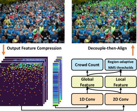
Figure 1: Our approach involves extracting output features from the detection outputs and refining them into 2D compressed matrices and 1D distribution vectors. These features are then encoded into local and global feature vectors to regress region-adaptive NMS thresholds and the crowd count. We select the final output bounding boxes using the decouple-then-align paradigm.

Although object detection may seem to meet the demands above, most relevant research views it pessimistically, especially in dense crowds [70, 54, 31, 48, 55]. First and foremost, compared to general object detection scenarios with bounding box annotations, most crowd analysis datasets only provide limited supervision in the form of point annotations. As a result, detection methods are restricted to using pseudo bounding boxes generated from point labels for training [45, 37, 57]. However, the inferior quality of these pseudo bounding boxes makes it difficult for neural networks to obtain effective supervision [48, 1].

Secondly, the density of crowds varies widely among images, ranging from zero to tens of thousands [45, 55, 71, 19, 47], and may vary across different regions in the same image, presenting a significant challenge in choosing the allowed overlapping region in Non-Maximum-Suppression (NMS). A fixed NMS threshold is often considered a hyperparameter, but it yields a large number of false positives within low-density crowds and false negatives within high-density crowds, as criticized in [48].

Thirdly, current detection methods adopt the detection-counting paradigm [40, 54] for crowd counting, where the number of humans is counted by the bounding boxes obtained from the detection output. However, the crowd detection task is extremely challenging without bounding box labels for training, resulting in a large number of mislabeled and unrecognized boxes in crowds [48, 55]. This inaccurate detection result makes the detection-counting paradigm perform poorly, yielding inferior counting results compared to density-based methods.

In this paper, we ask: Has the potential of object detection been fully discovered? Our findings suggest that crucial information from detection outputs, such as the size and confidence score of proposals and bounding boxes, are largely disregarded. This information can provide valuable insights into crowd-specific characteristics. For instance, in dense crowds, bounding boxes tend to be smaller with lower confidence scores due to occlusion, while sparse crowds tend to produce boxes with higher confidence scores.

To this end, we propose the a module on top of the Head of detection pipeline to leverage these underutilized detection outputs. We name this module as “Crowd Hat” because it can be adapted to different detection methods, just as a hat can be easily put on different heads. Specifically, we first introduce a mixed 2D-1D compression to refine both spatial and numerical distribution of output features from the detection pipeline. We further propose a NMS decoder to learn region-adaptive NMS thresholds from these features, which effectively reduces false positives under low-density regions and false negatives under high-density regions. Additionally, we use a decouple-then-align paradigm to improve counting performance by regressing the crowd count from output features and using this predicted count to guide the bounding box selection. Our Crowd Hat module can be integrated into various one-stage and two-stage object detection methods, bringing significant performance improvements for crowd analysis tasks. Extensive experiments on crowd counting, localization and detection demonstrate the effectiveness of our proposed approach.

Overall, the main contributions of our work can be summarized as the following:

• To the best of our knowledge, we are the first to consider detection outputs as valuable features in crowd analysis and propose the mixed 2D-1D compression to refine crowd-specific features from them.

• We introduce region-adaptive NMS thresholds and a decouple-then-align paradigm to mitigate major drawbacks of detection-based methods in crowd analysis.

• We evaluate our method on public benchmarks of crowd counting, localization, and detection tasks, showing our method can be adapted to different detection methods while achieving better performance.

2 Related Work

Density-Based Methods

Density-based methods have been continuously improved since first proposed in [23], for their superior performance and high efficiency in counting tasks. In this paradigm, a network is trained to map an input image to the crowd density map, thus the number of crowds is computed by summing the whole density map. While most advanced crowd counting methods are density-based [54, 40, 31, 28, 43, 20, 4, 56, 36, 46, 33, 63, 10], they tend to neglect spatial information [1, 45, 48], resulting in poor performance in individual pinpointing and bounding box provision for crowd heads [37, 45, 57].

Localization-Based Methods

To address the shortcomings of density-based methods in localization, researchers have proposed localization-based methods such as [1, 48, 32, 19, 58]. These methods achieve better performance in crowd localization and count crowds by summing the total number of points. However, while these methods outperform density-based methods in localization, their counting performance is generally worse [31, 52, 59], and they still fall short in meeting the needs of crowd detection [45, 57, 37].

Detection-Based Methods

Although detection-based methods are capable of resolving detection, localization, and counting tasks simultaneously, current research shows a pessimistic view of this paradigm. The fundamental capability of detection typically requires a significant number of bounding box labels for training, which are often unavailable in many crowd datasets [18, 19, 71]. Only a few methods, such as [37, 45, 57], attempt to train a detection network with pseudo box labels generated from point annotations. However, these methods suffer from inaccurate bounding boxes due to a fixed NMS process, which leads to too many false positives. As a result, detection-based methods generally perform worse in counting and localization tasks.

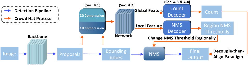
Figure 2: Overview of the Crowd Hat module. We adopt a two-stage detection method PSDNN as our detection pipeline for illustration.

3 Preliminary

Given a set of pair $(I,A)$ in the dataset, we define $I\in\mathbb{R}^{3\times H\times W}$ as the input image containing $N$ people and $A=\{a_{1},a_{2},...,a_{N}\}$ as the list of corresponding point annotations where $a_{k}=(a_{k}^{x},a_{k}^{y})$ is the center location of $k$ th head. $B=\{b_{1},b_{2},...,b_{k},...,b_{n}\}$ denotes the set of bounding boxes output by the network with $n$ predictions, and the $k$ th box is $b_{k}=(b_{k}^{x},b_{k}^{y},b_{k}^{w},b_{k}^{h},b_{k}^{c})$ where $b_{k}^{x}$ and $b_{k}^{y}$ is the coordinates of the center point, $b_{k}^{w},b_{k}^{h}$ is the width and height, and $b_{k}^{c}$ is the confidence of this box. For two-stage methods with region proposals, we denote $P=\{p_{1},p_{2},...,p_{k},...,p_{m}\}$ as the set of proposals with $m$ predictions. Likewise the $k$ th proposal is $p_{k}=(p_{k}^{x},p_{k}^{y},p_{k}^{w},p_{k}^{h},p_{k}^{c})$ with $p_{k}^{x},p_{k}^{y}$ as center coordinates, $p_{k}^{w},p_{k}^{h}$ as the width and height, and $p_{k}^{c}$ as the confidence of the proposal. Note that proposals and bounding boxes refer to the predictions before applying NMS and confidence score filtering.

All methods in our paper were trained using only point annotations to ensure fair comparisons [71, 19, 55]. Therefore, we generated pseudo bounding box labels from point annotations for training all detection methods, following common practice [45, 57, 37].

4 Methodology: Crowd Hat

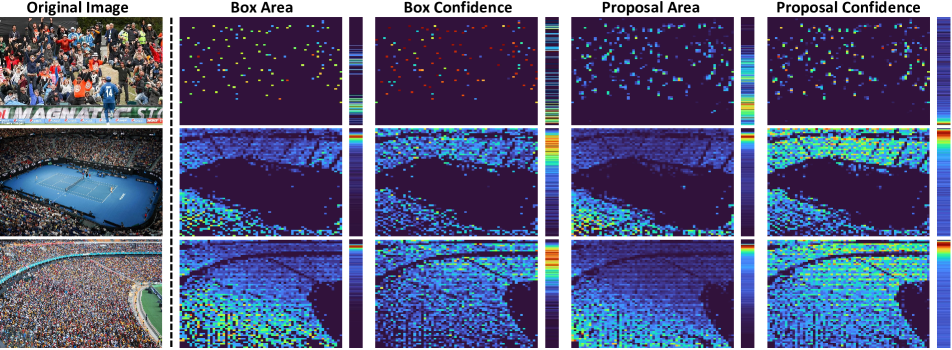
Figure 3: Visualization of output feature compression. We present the 2D compression matrices (left) and 1D distribution vectors (to the right) for each output feature. In the 1D distribution vectors, we use 0 to denote the top of the vector and 1 for the bottom. Additionally, we provide the original image in the leftmost column for reference. Zoom in for better visualization.

In our paper, we define detection outputs as the predicted bounding boxes and proposals from the detection pipeline. We find these outputs convey abundant crowd-specific information, making them valuable assets for crowd analysis tasks. In particular, we adopt two output features, namely “area size” and “confidence score” from detection outputs. Compared to feature maps extracted from convolution layers (CNN features), output features focus mostly on humans, the foreground of the image, and are considered relatively “pure” features for crowd analysis tasks. Therefore, we propose the Crowd Hat module to mine and utilize these output features, as shown in Figure 2. In this section, we use the two-stage detection method PSDNN [37] as the detection pipeline, and other one-stage detection methods [57, 45] can be easily adapted.

4.1 Output Feature Compression

The original format of detection outputs is a list of 5D vectors (see definitions in Section 3). Since the number of generated bounding boxes $n$ and the number of proposals $m$ vary among images, it is hard to pass these irregular vectors directly into neural networks. While mapping the output features directly back to the input image according to the center coordinates of detection outputs may seem like a trivial approach, the resulting feature maps will be too sparse to convey representative information since the number of predicted proposals or bounding boxes is far less than the number of pixels per image. To address this issue, we propose a mixed 2D-1D compression method to further refine the output features and obtain the spatial and numerical distribution of these crowd-specific information. We show visualization results of different features from the 2D-1D compression method in Figure 3.

4.1.1 2D Compression

To determine the spatial distribution of crowd density in an image, we propose 2D compression using a matrix $M\in R^{S\times S}$ to compress each output feature into patches. We map the proposal or bounding box to the input image based on its center coordinates, divide the image into $S\times S$ patches of equal height and width, and sum up each output feature located within each patch to obtain the corresponding element in the compression matrix $M$.

Consider compressing bounding box area using a compression matrix. To calculate the normalized area of the k-th bounding box, we multiply its width by the image height and divide the result by the product of the image’s width and height. This normalization step removes the impact of different image resolutions. Specifically, the normalized size is calculated as $\frac{b_{k}^{w}}{W}\cdot\frac{b_{k}^{h}}{H}$. We denote $M_{B}^{A}$ as the compressed matrix of bounding box area. Thus the formula yields:

$$M_{B}^{A}(i,j)=\sum_{k=1}^{n}[\left\lfloor\frac{b_{k}^{x}}{w_{0}}\right\rfloor=i]\cdot[\left\lfloor\frac{b_{k}^{y}}{h_{0}}\right\rfloor=j]\cdot\frac{b_{k}^{w}}{W}\cdot\frac{b_{k}^{h}}{H}$$ (1)

where two indicator functions $[\left\lfloor\frac{b_{k}^{x}}{w_{0}}\right\rfloor=i]$ and $[\left\lfloor\frac{b_{k}^{y}}{h_{0}}\right\rfloor=j]$ are equal to 1 only if the bounding box $b_{k}$ belongs to the patch indexed $(i,j)$ and 0 otherwise.

We use the notation $M_{B}^{C}$ to represent the compressed matrix of bounding box confidence scores, and $M_{P}^{A}$ and $M_{P}^{C}$ to represent the compressed matrices of proposal area size and confidence score, respectively. If a one-stage detection method does not generate proposals, we only use $M_{B}^{A}$ and $M_{B}^{C}$ as the compressed matrices. These matrices are formally defined as follows:

$$M_{B}^{C}(i,j)=\sum_{k=1}^{n}[\left\lfloor\frac{b_{k}^{x}}{w_{0}}\right\rfloor=i]\cdot[\left\lfloor\frac{b_{k}^{y}}{h_{0}}\right\rfloor=j]\cdot\sigma(b_{k}^{c})$$ (2)

$$M_{P}^{A}(i,j)=\sum_{k=1}^{m}[\left\lfloor\frac{p_{k}^{x}}{w_{0}}\right\rfloor=i]\cdot[\left\lfloor\frac{p_{k}^{y}}{h_{0}}\right\rfloor=j]\cdot\frac{p_{k}^{w}}{W}\cdot\frac{p_{k}^{h}}{H}$$ (3)

$$M_{P}^{C}(i,j)=\sum_{k=1}^{m}[\left\lfloor\frac{p_{k}^{x}}{w_{0}}\right\rfloor=i]\cdot[\left\lfloor\frac{p_{k}^{y}}{h_{0}}\right\rfloor=j]\cdot\sigma(p_{k}^{c})$$ (4)

4.1.2 1D Compression

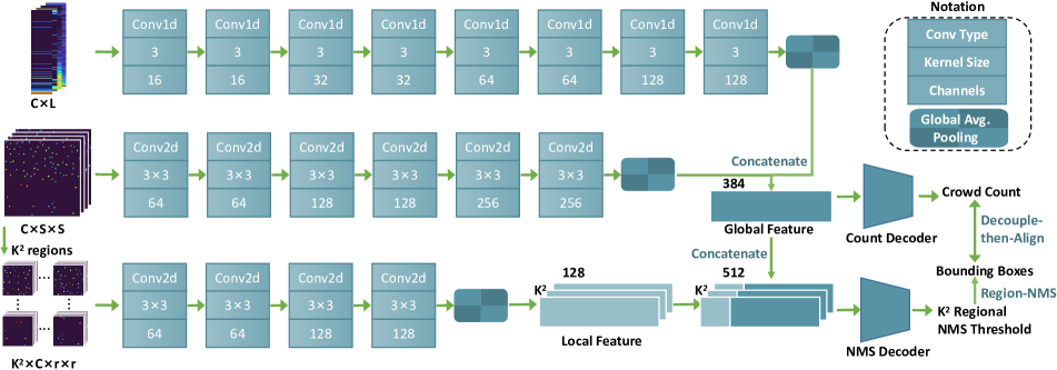
Figure 4: Detailed neural network structure of Crowd Hat module. The 2D compressed matrices and 1D distribution vectors are further transformed into global and local feature vectors via convolutional neural networks. Each convolution layer is followed by ReLU activation and a max-pooling layer, except for the last layer where we use global average pooling.

Crowd density varies greatly within and among images, with some images having densities ranging from zero to tens of thousands [45, 55, 71, 19, 47]. To determine the overall crowd density of an image, we propose a 1D compression method that finds the numerical distribution of output features within the image. For instance, a low overall distribution of output bounding box area sizes could indicate a high crowd density in the scene.

Our proposed 1D compression method works as follows: first, we normalize the confidence score and area size values to a range of 0 to 1. Next, we divide this range into $L$ discrete intervals, where the $i$-th interval is $[\frac{i}{L},\frac{i+1}{L})$. We then calculate the number of values that fall into each interval to form a histogram and obtain the numerical distribution where the $i$-th value of the histogram represents the number of values that fall into the interval $[\frac{i}{L},\frac{i+1}{L})$.

To normalize the output features into the interval of 0 to 1, we use a two-step process. First, we multiply the output feature by a scaling coefficient $\alpha\geq 1$, which is a hyperparameter. This step is necessary to ensure that the distribution of output features is distinguishable after nonlinear mapping. The raw values of area size and confidence score may be numerically congested, causing them to fall into the same interval or nearby intervals after nonlinear mapping. Second, we apply a nonlinear mapping function to the output feature to limit its range to [0, 1]. Note that area size is always greater than zero, while confidence can be either positive or negative, thus we use the sigmoid function $\sigma(x)$ for the confidence score and the hyperbolic tangent function $tanh(x)$ for the area size.

For instance, we transform the confidence score of the $k$-th bounding box, $b_{k}^{c}$, to $\sigma(b_{k}^{c}\cdot\alpha)$. This value falls into the interval $\sigma(b_{k}^{c}\cdot\alpha)/(\frac{1}{L})=\sigma(b_{k}^{c}\cdot\alpha)\cdot L$. We refer to the distribution vector of the bounding box confidence score as $V_{B}^{C}$ and its scaling coefficient as $\alpha_{B}^{C}$. The formula yields:

$$V_{B}^{C}(i)=\sum_{k=1}^{n}[\left\lfloor\sigma(b_{k}^{c}\cdot\alpha_{B}^{C})\cdot L\right\rfloor=i]$$ (5)

Similarly, we denote $V_{B}^{A}$ as the distribution vector of the bounding box area size and $V_{P}^{A},V_{P}^{C}$ as those of proposal area size and confidence score. The scaling coefficients for the corresponding output features are denoted as $\alpha_{B}^{A}$, $\alpha_{P}^{A}$, and $\alpha_{P}^{C}$, respectively. For one-stage detection methods that do not generate proposals, we only use $V_{B}^{A}$ and $V_{B}^{C}$ from the predicted bounding boxes. In formal terms:

$$V_{B}^{A}(i)=\sum_{k=1}^{n}[\left\lfloor tanh(\frac{b_{k}^{w}}{W}\cdot\frac{b_{k}^{h}}{H}\cdot\alpha_{B}^{A})\cdot L\right\rfloor=i]$$ (6)

$$V_{P}^{A}(i)=\sum_{k=1}^{m}[\left\lfloor tanh(\frac{p_{k}^{w}}{W}\cdot\frac{p_{k}^{h}}{H}\cdot\alpha_{P}^{A})\cdot L\right\rfloor=i]$$ (7)

$$V_{P}^{C}(i)=\sum_{k=1}^{m}[\left\lfloor\sigma(p_{k}^{c}\cdot\alpha_{P}^{C})\cdot L\right\rfloor=i]$$ (8)

4.2 Crowd Hat Network

To aggregate information from the different output features above, we stack the 2D compressed matrices to form a tensor $t_{2d}\in R^{C\times S\times S}$, and the distribution vectors from 1D compression are stacked to form a tensor $t_{1d}\in R^{C\times L}$. Here, $C$ is the number of output features used, with $C=4$ for two-stage methods and $C=2$ for one-stage methods. These tensors are then passed into our Crowd Hat network to obtain global and local features, as described below. The detailed structure is shown in Figure 4.

Global Feature To incorporate both the spatial information from $t_{2d}$ and the numerical distribution information from $t_{1d}$, we use 2D convolutions to further encode $t_{2d}$ and 1D convolutions for $t_{1d}$, as shown in Figure 4. After global average pooling, we concatenate both of them to form the global feature vector $F_{g}$.

Local Feature To capture the high variation of crowd density within an image and support our region-adaptive NMS, we introduce local features by dividing $t_{2d}$ into fixed-sized patches and encoding them using neural networks. We split $t_{2d}$ into $K\times K$ patches and then pass them through a 2D convolutional neural network with global average pooling to generate local feature vectors $[F_{l}^{1},F_{l}^{2},...F_{l}^{K^{2}}]$.

Table 1: Quantiative comparisons in crowd counting, best in bold, second in underline. All results are from corresponding papers or official implementations, and official records from NWPU-Crowd benchmark.

Method	Type	ShanghaiTech A		ShanghaiTech B		JHU-Crowd++		UCF-QNRF		NWPU-Crowd
		MAE $\downarrow$	RMSE $\downarrow$	MAE $\downarrow$	RMSE $\downarrow$	MAE $\downarrow$	RMSE $\downarrow$	MAE $\downarrow$	RMSE $\downarrow$	MAE $\downarrow$	RMSE $\downarrow$
Topo-Count[1] (AAAI 2020)	Localization-Based	61.2	104.6	7.8	13.7	60.9	267.4	89.0	159.0	107.8	438.5
P2P-Net [48] (ICCV 2021)		52.7	85.1	6.3	9.9	56.3	268.3	85.3	154.5	77.4	362.0
GL [53] (CVPR 2021)		61.3	95.4	7.3	11.7	59.9	259.5	84.3	147.5	79.3	346.1
CLTR[30] (ECCV 2022)		56.9	95.2	6.5	10.6	59.5	240.6	85.8	141.3	74.3	333.8
ADSCNet [2] (CVPR 2020)	Density-Based	55.4	97.7	6.4	11.3	-	-	71.3	132.5	-	-
SUA-Fully [41] (ICCV 2021)		66.9	125.6	12.3	17.9	80.1	305.3	119.2	213.3	111.7	443.2
MAN [31] (CVPR 2022)		56.8	90.3	-	-	53.4	209.9	77.3	131.5	76.5	323.0
CrowdFormer [68] (IJCAI 2022)		56.9	97.4	5.7	9.6	-	-	78.8	136.1	67.1	301.6
LSC-CNN [45] (TPAMI 2021)	Detection-Based	66.4	117.0	8.1	12.7	87.3	309.0	120.5	218.2	115.4	418.5
SDNet [57] (TIP 2021)		65.1	104.4	7.8	12.6	78.8	295.4	102.1	176.0	100.2	385.8
PSDNN [37] (CVPR 2019)		70.2	125.8	9.1	14.2	95.7	344.3	137.5	240.1	140.7	553.6
LSC-CNN + Crowd Hat (ours)	Detection-Based	60.2	95.7	7.1	11.3	63.0	270.9	84.7	150.2	90.6	336.6
SDNet + Crowd Hat (ours)		53.4	87.2	6.5	10.4	56.9	251.5	81.0	139.4	73.7	321.0
PSDNN + Crowd Hat (ours)		51.2	81.9	5.7	9.4	52.3	211.8	75.1	126.7	68.7	296.9

4.3 Region-Adaptive NMS Decoder

We propose a NMS Decoder to address the challenge of varying crowd densities across regions. The region-adaptive NMS approach learns optimal NMS thresholds for each region, maximizing F1 score with current pseudo bounding box labels. To determine the pseudo NMS threshold labels for each region $[T_{1},T_{2},...,T_{K^{2}}]$, we use a linear search algorithm, measuring model performance under different NMS thresholds ranging from 0 to 1 at a fixed step of $s$, and selecting the NMS threshold that leads to the highest F1 score for each region.

To train our NMS Decoder, we concatenate local and global features and pass them through an MLP, $P_{N}$, to generate region-adaptive NMS thresholds. We directly regress pseudo NMS threshold labels for training. The region NMS loss can be defined as follows:

$$\mathcal{L}_{nms}=\frac{1}{K^{2}}\sum_{i=1}^{K^{2}}|P_{N}(F_{l}^{i}\odot F_{g})-T_{i}|$$ (9)

where $\odot$ denotes concatenation.

During inference, we apply the learned pseudo NMS threshold labels from the NMS Decoder to perform region-adaptive NMS. For each region, we use the corresponding pseudo NMS threshold label as the NMS threshold to filter out redundant bounding boxes. Since different regions may have different crowd densities, the region-adaptive NMS can filter out more redundant bounding boxes in regions with high crowd density and retain more bounding boxes in regions with low crowd density, leading to better performance.

4.4 Decouple-then-Align Paradigm

Detection-based methods for crowd counting suffer from the drawback of utilizing a detection-counting paradigm [45, 37, 57], where crowd count is predicted by counting the number of output bounding boxes. This paradigm leads to entanglement between counting performance and detection and localization results, which is particularly problematic given that datasets typically provide only point annotations, resulting in limited supervision to train the detection pipeline.

To address this issue, we propose to decouple the detection and counting process by directly regressing the crowd count using global features $F_{g}$. Unlike some early methods that use CNN features for count regression, the output features we use provide valuable crowd-specific information, making them more suitable for direct count regression. We use a separate MLP, called the Count Decoder $P_{C}$, to predict the crowd count $\hat{n}=P_{C}(F_{g})$, which is supervised by the ground truth crowd count obtained from point annotations. The loss function is formulated as follows:

$$\mathcal{L}_{count}=|P_{C}(F_{g})-N|$$ (10)

However, using a separate count regression may cause confusion due to inconsistent results between the regression and detection process. The number of bounding boxes generated after NMS filtering $n_{c}$ may differ from the count output from the Count Decoder $\hat{n}$, leading to uncertainty about which number to reference. To address this issue, we prioritize the accuracy and reliability of the Count Decoder and select the min($\hat{n}$,$n_{c}$) bounding boxes with the highest confidences as the final results.

5 Experiments

Table 2: Comparisons in crowd localization, best in bold, second in underline. All other results except for ours are from corresponding papers or official implementations, and official records from NWPU-Crowd benchmark.

Method	Type	JHU-Crowd++				UCF-QNRF				NWPU-Crowd
		F1-m $\uparrow$	Pre $\uparrow$	Rec $\uparrow$		F1-m $\uparrow$	Pre $\uparrow$	Rec $\uparrow$		F1-m $\uparrow$	Pre $\uparrow$	Rec $\uparrow$
Topo-Count [1] (AAAI 2020)	Localization-Based	57.6	62.6	53.4		80.3	81.8	79.0		69.2	68.3	70.1
P2P-Net [48] (ICCV 2021)		61.7	65.7	58.2		82.8	83.4	82.2		71.2	72.9	69.5
GL [53] (CVPR 2021)		61.8	64.6	59.3		76.5	78.2	74.8		66.0	80.0	56.2
AutoScale [62] (IJCV 2022)		53.7	57.2	50.7		77.3	78.9	75.8		62.0	67.4	57.4
CLTR[30] (ECCV 2022)		-	-	-		82.2	80.0	80.1		69.4	67.6	68.5
LSC-CNN [45] (TPAMI 2021)	Detection-Based	52.5	55.6	49.8		74.1	74.6	73.5		59.3	67.1	53.4
SDNet [57] (TIP 2021)		56.2	61.3	52.0		78.0	78.9	77.2		63.7	65.1	62.4
PSDNN [37] (CVPR 2019)		50.2	53.7	47.1		67.0	63.6	70.8		53.7	53.3	54.1
LSC-CNN + Crowd Hat (ours)	Detection-Based	57.7	60.4	55.3		80.1	80.4	79.8		70.8	74.3	67.7
SDNet + Crowd Hat (ours)		64.3	68.0	61.1		83.5	84.0	83.1		75.9	74.0	77.8
PSDNN + Crowd Hat (ours)		65.9	72.6	60.3		86.2	85.9	86.6		78.2	78.2	78.3

Table 3: Comparisons in crowd detection, best in bold, second in underline.

Method	Easy $\uparrow$	Medium $\uparrow$	Hard $\uparrow$
CSR-A-thr [29] (CVPR 2018)	30.2	41.9	33.5
LSC-CNN [45] (TPAMI 2021)	40.5	62.1	46.2
PSDNN [37] (CVPR 2019)	60.5	60.5	39.6
SDNet [57] (TIP 2021)	75.8	71.0	64.4
LSC-CNN + Crowd Hat (ours)	68.4	72.3	59.7
PSDNN + Crowd Hat (ours)	81.5	78.1	66.5
SDNet + Crowd Hat (ours)	84.7	75.9	69.4

5.1 Implementation Details

The Crowd Hat module is decoupled from the detection pipeline and can be applied to a pre-trained detection model. Our framework is implemented on top of three detection-based methods, namely PSDNN [37], LSC-CNN [45], and SDNet [57]. During inference, relevant data such as $t_{2d}$, $t_{1d}$ (Section 4.2), and $[T_{1},T_{2},...,T_{K^{2}}]$ (Section 4.4) is saved to disk, while the detection pipeline’s weights remain fixed. The Crowd Hat network (Figure 4) is then trained using this data, with a spatial size of 64 for the 2D compressed matrix $S$ and a length of 256 intervals for the 1D distribution vector $L$. We extract local features by splitting the images into $K^{2}=16$ patches with a step for linear search $s$ set to 0.01. Our model is trained on 4 Nvidia RTX 3090 GPUs with a batch size of 16 for all datasets using the Adam optimizer with a learning rate of $1e-5$, over a period of 120 epochs for NWPU-Crowd dataset and 100 epoched for others.

5.2 Experimental Settings

We evaluate our methods for crowd analysis tasks, including detection, localization, and counting.

Crowd Detection

Our method is evaluated on the WIDER-Face validation set for crowd detection using average precision (AP) as the detection metric with an IOU set to 0.5, following standard practice [37, 45, 57].

Crowd Localization

We evaluated our approach on three public benchmarks: JHU-Crowd++[47], UCF-QNRF[19], and NWPU-Crowd [55]. We used Precision, Recall, and F-measure as evaluation metrics. For NWPU-Crowd and JHU-Crowd++, we followed the evaluation criteria in [55], which uses box labels for assessing successful matches. For UCF-QNRF, which does not have box labels, we evaluated at various distance thresholds (1 to 100 pixels) as per the standard practice in [19, 1].

Crowd Counting

In addition to datasets used for localization, we also performed comparisons on the ShanghaiTech dataset [71]. We evaluated the counting performance using the Mean Absolute Error (MAE) and Root Mean Squared Error (RMSE) metrics, which are widely used in prior work [70, 40, 54, 55].

Table 4: Ablation studies on counting, localization, and detection. We conduct counting and localization experiments under UCF-QNRF dataset and detection experiments under WIDER-Face dataset (Hard set). We adopt PSDNN [37], a two-stage detection based method as our baseline, which generates both proposals and bounding boxes.

Ablation	Method	Counting			Localization				Detection
		MAE $\downarrow$	RMSE $\downarrow$		F1-m $\uparrow$	Precision $\uparrow$	Recall $\uparrow$		AP $\uparrow$
Ablation I	CNN Features	129.3	222.8		68.1	67.3	68.9		41.2
	Output Features	75.1	126.7		86.2	85.9	86.6		66.5
Ablation II	Box Area	89.1	150.3		79.0	78.6	79.5		55.2
	Box Confidence	86.9	147.3		82.5	82.1	82.9		58.1
	Proposal Area	86.7	145.2		83.7	83.3	84.2		61.9
	Proposal Confidence	87.4	151.6		82.2	80.9	83.5		58.5
	All Output Features	75.1	126.7		86.2	85.9	86.6		66.5
Ablation III	Baseline	137.5	240.1		67.0	63.6	70.8		39.6
	Baseline + w/o Compression	103.6	171.0		72.4	71.8	73.1		46.8
	Baseline + 2D	82.1	138.3		83.8	83.2	84.4		62.8
	Baseline + 2D + 1D	75.1	126.7		86.2	85.9	86.6		66.5
Ablation IV	Baseline	137.5	240.1		67.0	63.6	70.8		39.6
	Baseline + Region Adaptive NMS	88.2	151.3		84.9	84.5	85.3		62.2
	Baseline + Decouple-then-Align	76.2	130.1		72.3	70.5	74.2		45.7
	Baseline + All	75.1	126.7		86.2	85.9	86.6		66.5

5.3 Comparison to State-of-the-Art

Crowd Counting

Table 1 shows quantitative results for counting across five datasets. Density-based methods generally perform best, while existing detection methods perform worst; however, our Crowd Hat greatly improves the counting performance of detection methods, making them competitive with state-of-the-art density-based methods. Notably, our PSDNN + Crowd Hat even outperforms some advanced density-based methods on certain datasets.

Crowd Localization

Our method’s evaluation under the crowd localization task is shown in Table 2. It significantly improves detection-based methods and achieves state-of-the-art performance across three datasets.

Crowd Detection

Our method significantly boost the performance of detection methods on the dense face detection dataset WIDER-Face, achieving state-of-the-art detection results across three test sets, as demonstrated in Table 3.

Table 5: Comparison of the model size (M), and Inference time (s / 100 images).

Method	Model Size	Inference Time
LSC-CNN [45]	35.08	57.73
LSC-CNN + Crowd Hat (ours)	36.71 (+4.6%)	59.64 (+3.3%)
SDNet [57]	40.04	193.54
SDNet + Crowd Hat (ours)	41.67 (+4.1%)	195.47 (+1.0%)
PSDNN [37]	47.51	14.35
PSDNN + Crowd Hat (ours)	49.14 (+3.4%)	16.38 (+14.1%)

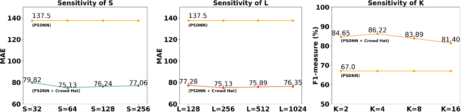
Figure 5: Studies on the sensitivity of hyperparameters on UCF-QNRF dataset.

5.4 Ablation Studies

Here, we study the effect of some of our key designs.

Output features vs. CNN Features

We compared output features to CNN features (the last feature map from the backbone network) in Ablation 1 of Table 4 to study their quality. By replacing the output features with CNN features while keeping the rest constant, we found that the output features perform significantly better than CNN features.

Study of selected features

In Ablation 2, we evaluated the effectiveness of each output feature used in our paper. Our results show that each output feature improves the performance of the detection baseline, and the best performance is achieved by aggregating all of these features.

Study of Output Feature Compression

In Ablation 3, we evaluated the effectiveness of 2D compressed matrices and 1D distribution vectors. All other modules were included in this experiment. We started by mapping the detection outputs back to the input image without compression as “Baseline + w/o Compression”. Our results show that directly using output features without compression only provides a negligible increase in performance. However, we found that adding 2D compression matrices resulted in increased performance in all experiments. Further addition of 1D distribution vectors boosted overall performance, demonstrating the effectiveness of both 2D and 1D compression.

Study of Region Adaptive NMS and Decouple-then-Align Paradigm

In Ablation 4, we evaluated the effectiveness of two important modules: Region Adaptive NMS and Decouple-then-Align Paradigm, using all output features with compression for all experiments. We found that adding Region Adaptive NMS resulted in performance increases for all tasks, particularly for Localization and Detection tasks. Decouple-then-Align Paradigm mainly boosted the performance of crowd counting task while also providing minor benefits for detection and localization tasks. The best performance was achieved by adding both modules.

Sensitivity of Hyperparameters

Figure 5 shows sensitivity experiments conducted on three important hyperparameters of PSDNN + Crowd Hat: the spatial dimension of the 2D compressed matrix $S$, the spatial dimension of the 1D compressed vector $L$, and the number of regions in the region-adaptive NMS threshold $K$. Specifically, counting experiments were conducted for $S$ and $L$, while a localization experiment was conducted for $K$ using the UCF-QNRF dataset. During testing of one hyperparameter, the others were fixed to their default settings as specified in the implementation details. The performance for various values of $S$ and $L$ remained relatively stable, with the best performance achieved when $S$ = 64 and $L$ = 256. For the hyperparameter $K$, the best performance was achieved with $K=4$.

Running Cost Evaluations

We compared the model size and inference time in Table 5 by processing all images into 1024 × 768 resolution and running the experiment on one RTX 3090 GPU. Our results show that after adding our Crowd Hat module, there was no significant increase in model size or inference time, indicating that our model is lightweight and can be easily adapted to different detection pipelines.

6 Conclusion

In this paper, we propose a Crowd Hat module to leverage underutilized output features from bounding boxes and proposals in the detection pipeline for crowd analysis tasks. Our extensive evaluations under three different crowd analysis tasks demonstrate the effectiveness of our approach and highlight the potential of using output features as valuable assets in crowd analysis.

limitations and future work.

We show that area size and confidence score have a strong correspondence with the crowd distribution, but there can be potential better features more effective. In addition, as the 1D compression is not differentiable, our model can not be trained in an end-to-end manner.

Appendix A Detailed Evaluation Metrics

Crowd Counting

Mean Absolute Error (MAE) and Root Mean Squared Error (RMSE) are widely used as counting metrics, and they are defined as follows:

$$MAE=\frac{1}{N}\sum_{i=1}^{n}\left|e_{i}-gt_{i}\right|$$ (11)

$$RMSE=\sqrt{\frac{1}{N}\sum_{i=1}^{n}(e_{i}-gt_{i})^{2}}$$ (12)

Here, $e_{i}$ and $gt_{i}$ represent the estimated count and ground truth count of crowds, respectively, and N is the total number of images.

Crowd Localization

F1 Measure, Precision, and Recall are commonly used as metrics for crowd localization, as proposed in [55]. We denote the two point sets of prediction results as $P_{p}$ and ground truth as $P_{g}$, and construct a Bipartite Graph $G_{p,s}$ for the two sets. Then, we compute the distance matrix of $P_{p}$ and $P_{g}$. If the distance between $p_{p}\in P_{p}$ and $p_{g}\in P_{g}$ is less than a predefined distance threshold $\sigma$, we consider $p_{p}$ and $p_{g}$ to be successfully matched, and obtain a boolean match matrix (True and False denote matched and non-matched) corresponding to each element of the distance matrix. Finally, by implementing the Hungarian algorithm, we obtain a Maximum Bipartite Matching for $G_{p,s}$. Based on the counts of True Positive (TP), False Positive (FP), and False Negative (FN), we can compute Precision (P), Recall (R), and F1 Measure ($F_{1}$) as follows:

$$P=\frac{TP}{TP+FP},R=\frac{TP}{TP+FN},F_{1}=\frac{2PR}{P+R}$$ (13)

Crowd Detection

Following standard practices, we adopt the average precision (AP) as the detection metric, with an Intersection over Union (IOU) threshold of 0.5.

Appendix B Datasets

WIDER-Face [69] is a dense face detection dataset consisting of 32,203 images and 393,703 face labels, which exhibit high variability in terms of scale, pose, and occlusion.

ShanghaiTech [71] consists of two independent subsets, Part A and Part B. Part A contains highly congested images collected from the Internet, while Part B is comprised of images taken from the busy streets of metropolitan areas in Shanghai.

UCF-QNRF [19] contains 1535 images, which exhibit a much wider range of crowd counts compared to the previous datasets, making it a more challenging dataset for crowd analysis

JHU-Crowd++ [47] is a large-scale unconstrained dataset that comprises a total of 4,372 images, containing 1,515,005 head annotations and captured under a variety of conditions. The dataset includes challenging images captured under various weather-based degradation, as well as some negative samples that may be detected as false positives.

NWPU-Crowd [55] is the largest crowd analysis dataset, consisting of 5,109 images and 2,133,375 annotated heads with varying crowd densities. For an authentic evaluation of crowd counting and localization, we report our results from the official website of NWPU-crowd.

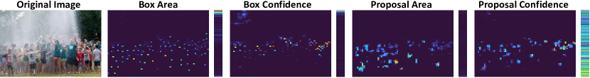
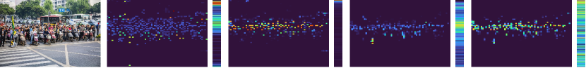
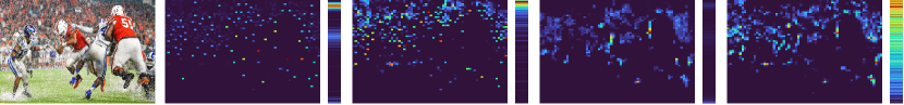
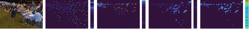
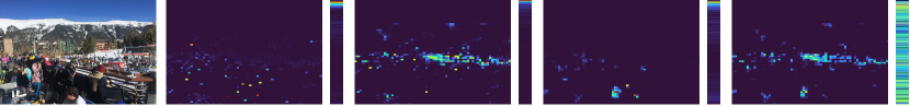
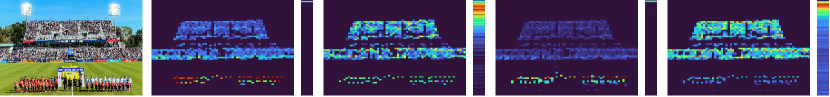
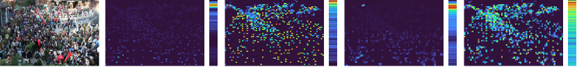
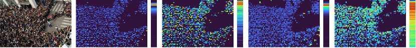
Figure 6: To visualize the 2D-1D feature compression, we present both the 2D compression matrices (on the left) and 1D distribution vectors (to their right) for each output feature. In the 1D distribution vectors, we denote 0 at the top and 1 at the bottom. Additionally, we include the original image in the leftmost column for reference. Zoom in for better visualization.

Appendix C Visualization of Compression

Figure 6 provides additional visualization of the 2D-1D feature compression achieved by the PSDNN + Crowd Hat. Heat map is adopted where 2D compression is on the left and 1D compression is on the right.

Appendix D Visualization of Detection

Figures 7 and 8 depict the detection results of SDNet with and without our proposed Crowd Hat module. Following the practice in [55, 37], we use green boxes to indicate true positives based on ground truth annotations, red boxes for false negatives, and yellow boxes for false positives, for better clarity.

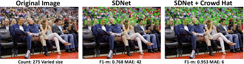
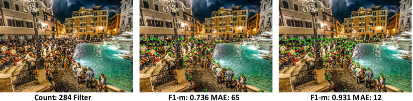
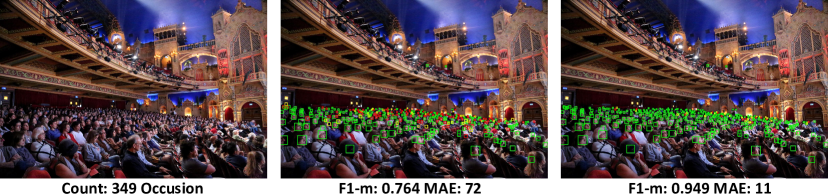
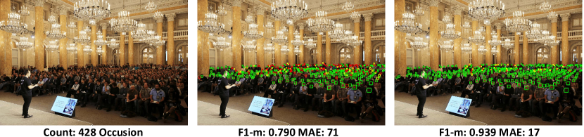
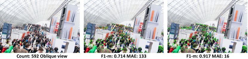
Figure 7: Visualization of Detection in Low Density Crowd.

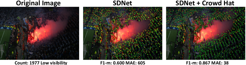
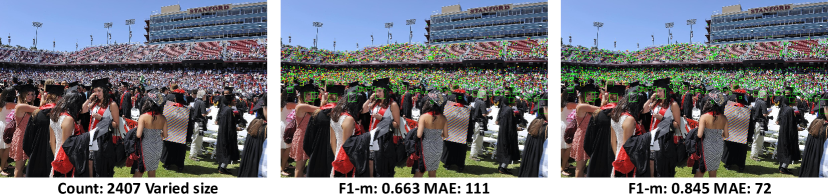
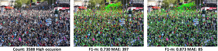
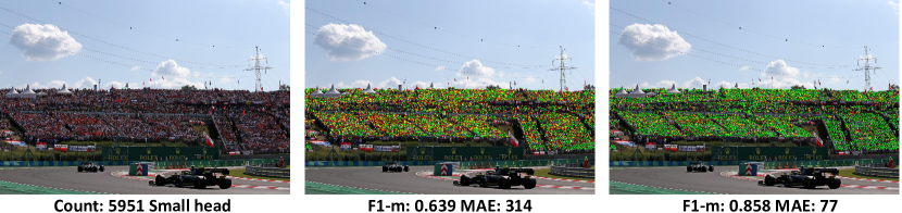
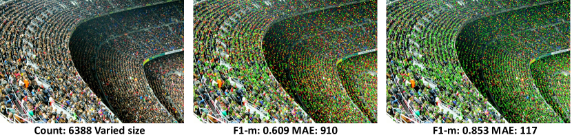
Figure 8: Visualization of Detection in High Density Crowd.

References

- [1] Shahira Abousamra, Minh Hoai, Dimitris Samaras, and Chao Chen. Localization in the crowd with topological constraints. In Thirty-Fifth AAAI Conference on Artificial Intelligence, AAAI 2021, Thirty-Third Conference on Innovative Applications of Artificial Intelligence, IAAI 2021, The Eleventh Symposium on Educational Advances in Artificial Intelligence, EAAI 2021, Virtual Event, February 2-9, 2021, pages 872–881. AAAI Press, 2021.
- [2] Shuai Bai, Zhiqun He, Yu Qiao, Hanzhe Hu, Wei Wu, and Junjie Yan. Adaptive dilated network with self-correction supervision for counting. In 2020 IEEE/CVF Conference on Computer Vision and Pattern Recognition, CVPR 2020, Seattle, WA, USA, June 13-19, 2020, pages 4593–4602. Computer Vision Foundation / IEEE, 2020.
- [3] Navaneeth Bodla, Bharat Singh, Rama Chellappa, and Larry S. Davis. Soft-nms - improving object detection with one line of code. In IEEE International Conference on Computer Vision, ICCV 2017, Venice, Italy, October 22-29, 2017, pages 5562–5570. IEEE Computer Society, 2017.
- [4] Xinkun Cao, Zhipeng Wang, Yanyun Zhao, and Fei Su. Scale aggregation network for accurate and efficient crowd counting. In Computer Vision - ECCV 2018, volume 11209 of Lecture Notes in Computer Science, pages 757–773. Springer, 2018.
- [5] A. B. Chan and N. Vasconcelos. Bayesian poisson regression for crowd counting. In 2009 IEEE 12th International Conference on Computer Vision (ICCV), pages 545–551, Los Alamitos, CA, USA, oct 2009. IEEE Computer Society.
- [6] Chao Chen, Xinhao Liu, Yiming Li, Li Ding, and Chen Feng. Deepmapping2: Self-supervised large-scale lidar map optimization. In Proceedings of the IEEE/CVF Conference on Computer Vision and Pattern Recognition, pages 9306–9316, 2023.
- [7] Ke Chen, Shaogang Gong, Tao Xiang, and Chen Change Loy. Cumulative attribute space for age and crowd density estimation. 06 2013.
- [8] Ke Chen, Chen Change Loy, Shaogang Gong, and Tao Xiang. Feature mining for localised crowd counting. 01 2012.
- [9] Yu Chen, Ying Tai, Xiaoming Liu, Chunhua Shen, and Jian Yang. Fsrnet: End-to-end learning face super-resolution with facial priors. In 2018 IEEE Conference on Computer Vision and Pattern Recognition, CVPR 2018, Salt Lake City, UT, USA, June 18-22, 2018, pages 2492–2501. Computer Vision Foundation / IEEE Computer Society, 2018.
- [10] Zhi-Qi Cheng, Jun-Xiu Li, Qi Dai, Xiao Wu, and Alexander G. Hauptmann. Learning spatial awareness to improve crowd counting. In 2019 IEEE/CVF International Conference on Computer Vision, ICCV 2019, Seoul, Korea (South), October 27 - November 2, 2019, pages 6151–6160. IEEE, 2019.
- [11] Jiankang Deng, Jia Guo, Niannan Xue, and Stefanos Zafeiriou. Arcface: Additive angular margin loss for deep face recognition. In IEEE Conference on Computer Vision and Pattern Recognition, CVPR 2019, Long Beach, CA, USA, June 16-20, 2019, pages 4690–4699. Computer Vision Foundation / IEEE, 2019.
- [12] Jiahua Dong, Yang Cong, Gan Sun, Bineng Zhong, and Xiaowei Xu. What can be transferred: Unsupervised domain adaptation for endoscopic lesions segmentation. In IEEE/CVF Conference on Computer Vision and Pattern Recognition (CVPR), pages 4022–4031, June 2020.
- [13] Junyu Gao, Tao Han, Yuan Yuan, and Qi Wang. Learning independent instance maps for crowd localization. arXiv preprint arXiv:2012.04164, 2020.
- [14] Kaiming He, Georgia Gkioxari, Piotr Dollár, and Ross B. Girshick. Mask R-CNN. In IEEE International Conference on Computer Vision, ICCV 2017, Venice, Italy, October 22-29, 2017, pages 2980–2988. IEEE Computer Society, 2017.
- [15] Jan Hendrik Hosang, Rodrigo Benenson, and Bernt Schiele. Learning non-maximum suppression. In 2017 IEEE Conference on Computer Vision and Pattern Recognition, CVPR 2017, Honolulu, HI, USA, July 21-26, 2017, pages 6469–6477. IEEE Computer Society, 2017.
- [16] Peiyun Hu and Deva Ramanan. Finding tiny faces. In The IEEE Conference on Computer Vision and Pattern Recognition (CVPR), July 2017.
- [17] Yutao Hu, Xiaolong Jiang, Xuhui Liu, Baochang Zhang, Jungong Han, Xianbin Cao, and David S. Doermann. Nas-count: Counting-by-density with neural architecture search. In Andrea Vedaldi, Horst Bischof, Thomas Brox, and Jan-Michael Frahm, editors, Computer Vision - ECCV 2020 - 16th European Conference, Glasgow, UK, August 23-28, 2020, Proceedings, Part XXII, volume 12367 of Lecture Notes in Computer Science, pages 747–766. Springer, 2020.
- [18] Haroon Idrees, Imran Saleemi, Cody Seibert, and Mubarak Shah. Multi-source multi-scale counting in extremely dense crowd images. In 2013 IEEE Conference on Computer Vision and Pattern Recognition, Portland, OR, USA, June 23-28, 2013, pages 2547–2554. IEEE Computer Society, 2013.
- [19] Haroon Idrees, Muhmmad Tayyab, Kishan Athrey, Dong Zhang, Somaya Al-Máadeed, Nasir M. Rajpoot, and Mubarak Shah. Composition loss for counting, density map estimation and localization in dense crowds. In Vittorio Ferrari, Martial Hebert, Cristian Sminchisescu, and Yair Weiss, editors, Computer Vision - ECCV 2018 - 15th European Conference, Munich, Germany, September 8-14, 2018, Proceedings, Part II, volume 11206 of Lecture Notes in Computer Science, pages 544–559. Springer, 2018.
- [20] Haroon Idrees, Muhmmad Tayyab, Kishan Athrey, Dong Zhang, Somaya Al-Máadeed, Nasir M. Rajpoot, and Mubarak Shah. Composition loss for counting, density map estimation and localization in dense crowds. In Vittorio Ferrari, Martial Hebert, Cristian Sminchisescu, and Yair Weiss, editors, Computer Vision - ECCV 2018 - 15th European Conference, Munich, Germany, September 8-14, 2018, Proceedings, Part II, volume 11206 of Lecture Notes in Computer Science, pages 544–559. Springer, 2018.
- [21] Wei Ji, Xi Li, Fei Wu, Zhijie Pan, and Yueting Zhuang. Human-centric clothing segmentation via deformable semantic locality-preserving network. IEEE Transactions on Circuits and Systems for Video Technology, 30(12):4837–4848, 2019.
- [22] Xiaoheng Jiang, Li Zhang, Mingliang Xu, Tianzhu Zhang, Pei Lv, Bing Zhou, Xin Yang, and Yanwei Pang. Attention scaling for crowd counting. In 2020 IEEE/CVF Conference on Computer Vision and Pattern Recognition, CVPR 2020, Seattle, WA, USA, June 13-19, 2020, pages 4705–4714. Computer Vision Foundation / IEEE, 2020.
- [23] Victor S. Lempitsky and Andrew Zisserman. Learning to count objects in images. In Advances in Neural Information Processing Systems 23: 24th Annual Conference on Neural Information Processing Systems 2010. Proceedings of a meeting held 6-9 December 2010, Vancouver, British Columbia, Canada, pages 1324–1332. Curran Associates, Inc., 2010.
- [24] Gil Levi and Tal Hassner. Age and gender classification using convolutional neural networks. In 2015 IEEE Conference on Computer Vision and Pattern Recognition Workshops, CVPR Workshops 2015, Boston, MA, USA, June 7-12, 2015, pages 34–42. IEEE Computer Society, 2015.
- [25] Gaotang Li, Marlena Duda, Xiang Zhang, Danai Koutra, and Yujun Yan. Interpretable sparsification of brain graphs: Better practices and effective designs for graph neural networks. KDD ’23, page 1223–1234, New York, NY, USA, 2023. Association for Computing Machinery.
- [26] Jian Li, Yabiao Wang, Changan Wang, Ying Tai, Jianjun Qian, Jian Yang, Chengjie Wang, Jilin Li, and Feiyue Huang. DSFD: dual shot face detector. In IEEE Conference on Computer Vision and Pattern Recognition, CVPR 2019, Long Beach, CA, USA, June 16-20, 2019, pages 5060–5069. Computer Vision Foundation / IEEE, 2019.
- [27] Yicong Li, Xiang Wang, Junbin Xiao, Wei Ji, and Tat-Seng Chua. Invariant grounding for video question answering. In Proceedings of the IEEE/CVF Conference on Computer Vision and Pattern Recognition, pages 2928–2937, 2022.
- [28] Yuhong Li, Xiaofan Zhang, and Deming Chen. Csrnet: Dilated convolutional neural networks for understanding the highly congested scenes. In 2018 IEEE Conference on Computer Vision and Pattern Recognition, CVPR 2018, Salt Lake City, UT, USA, June 18-22, 2018, pages 1091–1100. Computer Vision Foundation / IEEE Computer Society, 2018.
- [29] Yuhong Li, Xiaofan Zhang, and Deming Chen. Csrnet: Dilated convolutional neural networks for understanding the highly congested scenes. In 2018 IEEE Conference on Computer Vision and Pattern Recognition, CVPR 2018, Salt Lake City, UT, USA, June 18-22, 2018, pages 1091–1100. Computer Vision Foundation / IEEE Computer Society, 2018.
- [30] Dingkang Liang, Wei Xu, and Xiang Bai. An end-to-end transformer model for crowd localization. European Conference on Computer Vision, 2022.
- [31] Hui Lin, Zhiheng Ma, Rongrong Ji, Yaowei Wang, and Xiaopeng Hong. Boosting crowd counting via multifaceted attention. In IEEE Conference on Computer Vision and Pattern Recognition, CVPR, 2022.
- [32] Chenchen Liu, Xinyu Weng, and Yadong Mu. Recurrent attentive zooming for joint crowd counting and precise localization. In IEEE Conference on Computer Vision and Pattern Recognition, CVPR 2019, Long Beach, CA, USA, June 16-20, 2019, pages 1217–1226. Computer Vision Foundation / IEEE, 2019.
- [33] Ning Liu, Yongchao Long, Changqing Zou, Qun Niu, Li Pan, and Hefeng Wu. Adcrowdnet: An attention-injective deformable convolutional network for crowd understanding. In IEEE Conference on Computer Vision and Pattern Recognition, CVPR 2019, Long Beach, CA, USA, June 16-20, 2019, pages 3225–3234. Computer Vision Foundation / IEEE, 2019.
- [34] Songtao Liu, Di Huang, and Yunhong Wang. Adaptive NMS: refining pedestrian detection in a crowd. In IEEE Conference on Computer Vision and Pattern Recognition, CVPR 2019, Long Beach, CA, USA, June 16-20, 2019, pages 6459–6468. Computer Vision Foundation / IEEE, 2019.
- [35] Wei Liu, Shengcai Liao, Weiqiang Ren, Weidong Hu, and Yinan Yu. High-level semantic feature detection: A new perspective for pedestrian detection. In IEEE Conference on Computer Vision and Pattern Recognition, CVPR 2019, Long Beach, CA, USA, June 16-20, 2019, pages 5187–5196. Computer Vision Foundation / IEEE, 2019.
- [36] Weizhe Liu, Mathieu Salzmann, and Pascal Fua. Context-aware crowd counting. In IEEE Conference on Computer Vision and Pattern Recognition, CVPR 2019, Long Beach, CA, USA, June 16-20, 2019, pages 5099–5108. Computer Vision Foundation / IEEE, 2019.
- [37] Yuting Liu, Miaojing Shi, Qijun Zhao, and Xiaofang Wang. Point in, box out: Beyond counting persons in crowds. In IEEE Conference on Computer Vision and Pattern Recognition, CVPR 2019, Long Beach, CA, USA, June 16-20, 2019, pages 6469–6478. Computer Vision Foundation / IEEE, 2019.
- [38] Chenyang Ma, Xinchi Qiu, Daniel Beutel, and Nicholas Lane. Gradient-less federated gradient boosting tree with learnable learning rates. EuroMLSys ’23, page 56–63, New York, NY, USA, 2023. Association for Computing Machinery.
- [39] Chenyang Ma, Xinchi Qiu, Daniel J. Beutel, and Nicholas D. Lane. Gradient-less federated gradient boosting tree with learnable learning rates. In Proceedings of the 3rd Workshop on Machine Learning and Systems, EuroMLSys 2023, Rome, Italy, 8 May 2023, pages 56–63. ACM, 2023.
- [40] Zhiheng Ma, Xing Wei, Xiaopeng Hong, and Yihong Gong. Bayesian loss for crowd count estimation with point supervision. In 2019 IEEE/CVF International Conference on Computer Vision, ICCV 2019, Seoul, Korea (South), October 27 - November 2, 2019, pages 6141–6150. IEEE, 2019.
- [41] Yanda Meng, Hongrun Zhang, Yitian Zhao, Xiaoyun Yang, Xuesheng Qian, Xiaowei Huang, and Yalin Zheng. Spatial uncertainty-aware semi-supervised crowd counting. In 2021 IEEE/CVF International Conference on Computer Vision, ICCV 2021, Montreal, QC, Canada, October 10-17, 2021, pages 15529–15539. IEEE, 2021.
- [42] Yasiru Ranasinghe, Nithin Gopalakrishnan Nair, W. G. C. Bandara, and Vishal M. Patel. Diffuse-denoise-count: Accurate crowd-counting with diffusion models. ArXiv, abs/2303.12790, 2023.
- [43] Viresh Ranjan, Hieu M. Le, and Minh Hoai. Iterative crowd counting. In Vittorio Ferrari, Martial Hebert, Cristian Sminchisescu, and Yair Weiss, editors, Computer Vision - ECCV 2018 - 15th European Conference, Munich, Germany, September 8-14, 2018, Proceedings, Part VII, volume 11211 of Lecture Notes in Computer Science, pages 278–293. Springer, 2018.
- [44] Shaoqing Ren, Kaiming He, Ross B. Girshick, and Jian Sun. Faster R-CNN: towards real-time object detection with region proposal networks. IEEE Trans. Pattern Anal. Mach. Intell., 39(6):1137–1149, 2017.
- [45] Deepak Babu Sam, Skand Vishwanath Peri, Mukuntha Narayanan Sundararaman, Amogh Kamath, and R. Venkatesh Babu. Locate, size, and count: Accurately resolving people in dense crowds via detection. IEEE Trans. Pattern Anal. Mach. Intell., 43(8):2739–2751, 2021.
- [46] Miaojing Shi, Zhaohui Yang, Chao Xu, and Qijun Chen. Revisiting perspective information for efficient crowd counting. In IEEE Conference on Computer Vision and Pattern Recognition, CVPR 2019, Long Beach, CA, USA, June 16-20, 2019, pages 7279–7288. Computer Vision Foundation / IEEE, 2019.
- [47] Vishwanath A. Sindagi, Rajeev Yasarla, and Vishal M. Patel. JHU-CROWD++: large-scale crowd counting dataset and A benchmark method. CoRR, abs/2004.03597, 2020.
- [48] Qingyu Song, Changan Wang, Zhengkai Jiang, Yabiao Wang, Ying Tai, Chengjie Wang, Jilin Li, Feiyue Huang, and Yang Wu. Rethinking counting and localization in crowds: A purely point-based framework. In 2021 IEEE/CVF International Conference on Computer Vision, ICCV 2021, Montreal, QC, Canada, October 10-17, 2021, pages 3345–3354. IEEE, 2021.
- [49] Ramana Sundararaman, Cedric De Almeida Braga, Éric Marchand, and Julien Pettré. Tracking pedestrian heads in dense crowd. In IEEE Conference on Computer Vision and Pattern Recognition, CVPR 2021, virtual, June 19-25, 2021, pages 3865–3875. Computer Vision Foundation / IEEE, 2021.
- [50] Ramana Sundararaman, Cedric De Almeida Braga, Éric Marchand, and Julien Pettré. Tracking pedestrian heads in dense crowd. In IEEE Conference on Computer Vision and Pattern Recognition, CVPR 2021, virtual, June 19-25, 2021, pages 3865–3875. Computer Vision Foundation / IEEE, 2021.
- [51] Xu Tang, Daniel K. Du, Zeqiang He, and Jingtuo Liu. Pyramidbox: A context-assisted single shot face detector. In Vittorio Ferrari, Martial Hebert, Cristian Sminchisescu, and Yair Weiss, editors, Computer Vision - ECCV 2018, volume 11213 of Lecture Notes in Computer Science, pages 812–828. Springer, 2018.
- [52] Ye Tian, Xiangxiang Chu, and Hongpeng Wang. Cctrans: Simplifying and improving crowd counting with transformer. CoRR, abs/2109.14483, 2021.
- [53] Jia Wan, Ziquan Liu, and Antoni B. Chan. A generalized loss function for crowd counting and localization. In IEEE Conference on Computer Vision and Pattern Recognition, CVPR 2021, virtual, June 19-25, 2021, pages 1974–1983. Computer Vision Foundation / IEEE, 2021.
- [54] Boyu Wang, Huidong Liu, Dimitris Samaras, and Minh Hoai Nguyen. Distribution matching for crowd counting. In NeurIPS 2020, 2020.
- [55] Qi Wang, Junyu Gao, Wei Lin, and Xuelong Li. Nwpu-crowd: A large-scale benchmark for crowd counting and localization. IEEE Trans. Pattern Anal. Mach. Intell., 43(6):2141–2149, 2021.
- [56] Qi Wang, Junyu Gao, Wei Lin, and Yuan Yuan. Learning from synthetic data for crowd counting in the wild. In IEEE Conference on Computer Vision and Pattern Recognition, CVPR 2019, Long Beach, CA, USA, June 16-20, 2019, pages 8198–8207. Computer Vision Foundation / IEEE, 2019.
- [57] Yi Wang, Junhui Hou, Xinyu Hou, and Lap-Pui Chau. A self-training approach for point-supervised object detection and counting in crowds. IEEE Trans. Image Process., 30:2876–2887, 2021.
- [58] Yi Wang, Xinyu Hou, and Lap-Pui Chau. Dense point prediction: A simple baseline for crowd counting and localization. In 2021 IEEE International Conference on Multimedia & Expo Workshops (ICMEW), pages 1–6. IEEE, 2021.
- [59] Xing Wei, Yuanrui Kang, Jihao Yang, Yunfeng Qiu, Dahu Shi, Wenming Tan, and Yihong Gong. Scene-adaptive attention network for crowd counting. CoRR, abs/2112.15509, 2021.
- [60] Shaokai Wu, Zhaogeng Liu, Wencheng Pei, Jianbo Hong, and Zhanshan Li. Faster, lighter, robuster: A weakly-supervised crowd analysis enhancement network and a generic feature extraction framework. In Proceedings of the IEEE/CVF Conference on Computer Vision and Pattern Recognition (CVPR) Workshops, pages 4050–4059, June 2022.
- [61] Haipeng Xiong, Hao Lu, Chengxin Liu, Liang Liu, Zhiguo Cao, and Chunhua Shen. From open set to closed set: Counting objects by spatial divide-and-conquer. In 2019 IEEE/CVF International Conference on Computer Vision, ICCV 2019, Seoul, Korea (South), October 27 - November 2, 2019, pages 8361–8370. IEEE, 2019.
- [62] Chenfeng Xu, Dingkang Liang, Yongchao Xu, Song Bai, Wei Zhan, Xiang Bai, and Masayoshi Tomizuka. Autoscale: Learning to scale for crowd counting. Int. J. Comput. Vis., 130(2):405–434, 2022.
- [63] Chenfeng Xu, Kai Qiu, Jianlong Fu, Song Bai, Yongchao Xu, and Xiang Bai. Learn to scale: Generating multipolar normalized density maps for crowd counting. In 2019 IEEE/CVF International Conference on Computer Vision, ICCV 2019, Seoul, Korea (South), October 27 - November 2, 2019, pages 8381–8389. IEEE, 2019.
- [64] Yujun Yan, Gao Li, and Danai Koutra. Size generalizability of graph neural networks on biological data: Insights and practices from the spectral perspective. ArXiv, abs/2305.15611, 2023.
- [65] Fengyu Yang and Chenyang Ma. Sparse and complete latent organization for geospatial semantic segmentation. In Proceedings of the IEEE/CVF Conference on Computer Vision and Pattern Recognition (CVPR), pages 1809–1818, June 2022.
- [66] Fengyu Yang, Chenyang Ma, Jiacheng Zhang, Jing Zhu, Wenzhen Yuan, and Andrew Owens. Touch and go: Learning from human-collected vision and touch. Neural Information Processing Systems (NeurIPS) - Datasets and Benchmarks Track, 2022.
- [67] Jian Yang, Lei Luo, Jianjun Qian, Ying Tai, Fanlong Zhang, and Yong Xu. Nuclear norm based matrix regression with applications to face recognition with occlusion and illumination changes. IEEE Trans. Pattern Anal. Mach. Intell., 39(1):156–171, 2017.
- [68] Shaopeng Yang, Weiyu Guo, and Yuheng Ren. Crowdformer: An overlap patching vision transformer for top-down crowd counting. In IJCAI, 2022.
- [69] Shuo Yang, Ping Luo, Chen Change Loy, and Xiaoou Tang. WIDER FACE: A face detection benchmark. In 2016 IEEE Conference on Computer Vision and Pattern Recognition, CVPR 2016, Las Vegas, NV, USA, June 27-30, 2016, pages 5525–5533. IEEE Computer Society, 2016.
- [70] Yingying Zhang, Desen Zhou, Siqin Chen, Shenghua Gao, and Yi Ma. Single-image crowd counting via multi-column convolutional neural network. In 2016 IEEE Conference on Computer Vision and Pattern Recognition, CVPR 2016, Las Vegas, NV, USA, June 27-30, 2016, pages 589–597. IEEE Computer Society, 2016.
- [71] Yingying Zhang, Desen Zhou, Siqin Chen, Shenghua Gao, and Yi Ma. Single-image crowd counting via multi-column convolutional neural network. In 2016 IEEE Conference on Computer Vision and Pattern Recognition, CVPR 2016, Las Vegas, NV, USA, June 27-30, 2016, pages 589–597. IEEE Computer Society, 2016.
- [72] Hanbin Zhao, Fengyu Yang, Xinghe Fu, and Xi Li. Rbc: Rectifying the biased context in continual semantic segmentation. In European Conference on Computer Vision, pages 55–72. Springer, 2022.