Reanalysis of the $\beta-\bar{\nu_{e}}$ angular correlation measurement aSPECT with new constraints on Fierz interference

Abstract

On the basis of revisions of some of the systematic errors, we reanalyzed the measurement of the electron-antineutrino angular correlation ($a$ coefficient) in free neutron beta decay from the aSPECT experiment. With $a=-0.10402(82)$ the new value differs only marginally from the one published in 2020. The experiment also has sensitivity to $b$, the Fierz interference term. From a correlated $(b,a)$ fit to the proton recoil spectrum, we derive a limit of $b=-0.0098(193)$ which translates into a somewhat improved 90% CL region of $-0.041\leq b\leq 0.022$ on this hypothetical term.

The aSPECT experiment [1, 2, 3] has the goal to determine the ratio of the weak axial-vector and vector coupling constants $\lambda=g_{\text{A}}/g_{\text{V}}$ from a measurement of the $\beta-\bar{\nu_{e}}$ angular correlation in neutron decay. The $\beta$-decay rate when observing only the electron and neutrino momenta and the neutron spin and neglecting a T-violating term is given by [4]

$$d^{3}\Gamma= G_{\text{F}}^{2}V_{\text{ud}}^{2}\left(1+3\lambda^{2}\right)p_{e}E_{e}\left(E_{0}-E_{e}\right)^{2}$$

$$\cdot\left(1+a\frac{\vec{p_{e}}\cdot\vec{p_{\nu}}}{E_{e}E_{\nu}}+b\frac{m_{e}}{E_{e}}+\frac{\vec{\sigma_{n}}}{\sigma_{n}}\cdot\left[A\frac{\vec{p_{e}}}{E_{e}}+B\frac{\vec{p_{\nu}}}{E_{\nu}}\right]\right)$$

$$\cdot dE_{e}d\Omega_{e}d\Omega_{\nu}$$ (1)

with $\vec{p_{e}}$, $\vec{p_{\nu}}$, $E_{e}$, $E_{\nu}$ being the momenta and total energies of the beta electron and the electron-antineutrino, $m_{e}$ the mass of the electron, $G_{\text{F}}$ the Fermi constant, $V_{\text{ud}}$ the first element of the Cabbibo-Kobayashi-Maskawa (CKM) matrix, $E_{0}$ the total energy available in the transition, and $\vec{\sigma_{n}}$ the spin of the neutron. The quantity $b$ is the Fierz interference coefficient. It vanishes in the purely vector axial-vector ($V-A$) interaction of the SM since it requires left-handed scalar ($S$) and tensor ($T$) interactions (see below). The correlation coefficients $a$ and $A$ ($\beta$-asymmetry parameter [5, 6]) are most sensitive to $\lambda$ and are used for its determination. The SM dependence of the beta-neutrino angular correlation coefficient $a$ on $\lambda$ is given by [4, 7, 8]

$$a=\frac{1-|\lambda|^{2}}{1+3|\lambda|^{2}}.$$ (2)

In short, at aSPECT the $a$ coefficient is inferred from the energy spectrum of the recoiling protons from the $\beta$ decay of free neutrons. The shape of this spectrum is sensitive to $a$ and it is measured in $4\pi$ by the aSPECT spectrometer using magnetic adiabatic collimation with an electrostatic filter (MAC-E filter) [9, 10]. This technique in general offers a high luminosity combined with a well-defined energy resolution at the same time. In order to extract a reliable value of $a$, any effect that changes the shape of the proton energy spectrum, or to be more specific: the integral of the product of the recoil energy spectrum and the spectrometer transmission function, has to be understood and quantified precisely. With the analysis of all known sources of systematic errors at that time and their inclusion in the final result by means of a global fit, the aSPECT collaboration published the value $a=-0.10430(84)$ [11]. From this, the ratio of axial-vector to vector coupling constants was derived giving $|\lambda|=1.2677(28)$. In the meantime, new aspects have emerged in the quantitative evaluation of some of the systematic errors that require a reanalysis of the data. Specifically, this concerns a) backscattering and below threshold losses in the detector (section IV G in [11]) and b) effective retardation voltage $<U_{\text{A}}>$ of the electrostatic filter (section IV D in [11]).

Backscattering and below threshold losses: Whereas the amount of electron-hole pair production in amorphous solids by a penetrating proton can be determined rather accurately with the binary collision code TRIM [12] (used in [11]), the calculation of the ionization depth profile in crystalline solids $E_{\text{ion.}}^{\text{C-TRIM}}(z)$ is more complicated due to channeling effects that TRIM doesn’t attempt to take into account. In our reanalysis we simulated the slowing down of protons in our silicon drift detector (SDD) (processed on a $\left<100\right>$-oriented Si wafer) by the program Crystal-TRIM originally developed in order to describe ion implantation into crystalline solids with several amorphous overlayers [13, 14] (in our case: a 30 nm thick aluminum overlayer including its 4 nm thick alumina layer [15] on top). The range of applicability of this code was studied by comparing with existing molecular dynamics simulations (see Fig. 6 in [16]), i.e., the depth profiles of 10 keV H ions on Si (diamond structure). With Crystal-TRIM good agreement (5%) was obtained for the parameter $C_{\text{el}}=0.65$ in the semiempirical formula for the local electronic energy loss [14].

The procedure to derive the calculated pulse heights $\propto E_{\text{eff~{}ion.}}^{\text{C-TRIM}}$ from many simulated proton events using Crystal-TRIM followed the same scheme as described in section IV G of [11] with the effective deposited ionization energy of each proton given by

$$E_{\text{eff~{}ion.}}^{\text{C-TRIM}}=\sum_{i}E_{\text{ion.}}^{\text{C-TRIM}}(z_{i})f_{\text{CCE}}^{\{\overline{par}\}}(z_{i})~{}~{}.$$ (3)

$f_{\text{CCE}}^{\{\overline{par}\}}(z_{i})$ is the charge collection efficiency for this type of detector [18] at depth ($z_{i}$). Protons with initial kinetic energy $T$ and relevant for aSPECT ($15~{}\text{keV}<(E_{\text{kin}}=15~{}\text{keV}+T)<15.75~{}\text{keV}$) have a very short range in the detector: maximum penetration depth of 516 nm (extreme case of channeling). The respective penetration depths were divided into bins of 3 nm and the deposited ionization energy per bin was determined including the amorphous overlayer with $f_{\text{CCE}}^{\{\overline{par}\}}(z_{i}<30~{}\text{nm})=0$. The physical ($E_{\text{kin}}$,$\alpha$) distributions of protons with energy $E_{\text{kin}}$ impinging on pad 2 and pad 3 of the SDD (impact angle $\alpha$) were extracted from particle tracking simulations. Protons with $\left<100\right>$ axial channeling incidence are rare, since they have to pass the amorphous overlayer of 30 nm that leads to de-channeling [19] (critical angle of channeling incidence $\alpha_{\text{crit}}^{\left<100\right>}\leq 3^{o}$ [16, 20]). As the impact angle of protons spans the range of $0<\alpha<20^{\circ}$ , channeling occurs preferentially on high-index axial and planar channels although the probability for the individual process is strongly reduced.
In our simulation of fractional losses [11] we have also stated that backscattered protons may return to the detector after motion reversal due to the electrostatic potential of the analyzing plane electrode of the aSPECT spectrometer. Those protons hit the detector again with the energy and angle to the normal they had when leaving the overlayer. Therefore, all possible hits of a proton due to backscattering were taken into account by adding the collected charge from all hits in the active region of the detector. In the meantime, we have realized that this is only partially correct: As J. Phillips [21] has shown, when low-energy hydrogen ions ($\text{H}^{+}$) pass through materials such as aluminum or more precisely: the 4 nm thin alumina top layer, electrons are captured or lost from the ions and particles of positive ($\text{H}^{+}$), neutral ($\text{H}^{0}$), and negative charge ($\text{H}^{-}$) arise. The two latter ones do not hit the detector a second time. The energy dependence of the percentage of positive components ($\text{H}^{+}$) is tabulated in [21] and can be approximated by a straight line ($\text{H}^{+}=8\%+E_{\text{kin}}^{{}^{\prime}}\cdot 1.674\%/\text{keV}$) in the energy range $4~{}\text{keV}<E_{\text{kin}}^{{}^{\prime}}<16~{}\text{keV}$ of interest.
Similar to what is displayed in Fig. 21 of [11], experimental and simulated pulse height spectra are compared. In each case the energy value at the maximum of the experimental spectrum was set equal to the corresponding theoretical value. Moreover, the theoretical spectra were folded with a normalized Gaussian distribution (120 eV FWHM). The FWHM-value corresponds to the intrinsic energy resolution derived in Ref. [22] for this type of SDD and includes the fluctuations of the charge collection efficiency parameters from their mean values $\{\overline{par}\}$. This procedure allows us to calculate the below-threshold losses including the events with no energy deposition inside the detector.
Fig. 1 shows the retardation voltage dependence of the fractional losses for the two detector pads. In both cases a cubic spline interpolation was used to describe the simulated events. In total, channeling and the inclusion of the alumina top layer do not significantly influence the spectral shape of the undetected protons, as the comparison with Fig. 22 in [11] shows. The higher fractional losses of $\approx 35\%$ (shape independent) have no effect on the final result due to normalization ($N_{0}$).

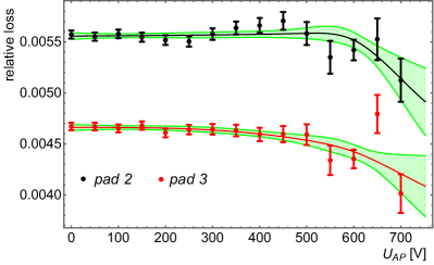
Figure 1: Fraction of undetected protons (both for pad 2 and pad 3 of the SDD) of the integral proton spectrum whose corresponding pulse heights fall below the threshold of the DAQ system (details see section IV G of [11]). The $U_{\text{AP}}$ dependence of the simulated losses can be described by a cubic spline function (solid line) and is shown together with the $1\sigma$ error predicted by the global fit (green band).

Effective retardation voltage $\left<U_{\text{A}}\right>$: Like the magnetic field ratio $r_{\text{B}}=B_{\text{A}}/B_{0}$, where $B_{0}$ and $B_{\text{A}}$ are the respective magnetic fields at the place of emission and retardation, the retardation voltage $U_{\text{AP}}$ directly enters the spectrometer’s adiabatic transmission function [2] given by

$$\begin{split}F_{\text{tr}}&(T,U_{\text{AP}},r_{\text{B}})\\ &=\left\{\begin{array}[]{ll}{0}&\text{if }T\leq eU_{\text{AP}}\\ {1-\sqrt{1-\frac{T-eU_{\text{AP}}}{r_{\text{B}}T}}}&\text{if }eU_{\text{AP}}<T<\frac{eU_{\text{AP}}}{1-r_{\text{B}}}\\ {1}&\text{if }T>\frac{eU_{\text{AP}}}{1-r_{\text{B}}}\\ \end{array}\right.\end{split}$$ (4)

The inhomogeneities of the potential in the decay volume (DV) and the analyzing plane (AP) region result in a slight shift $\Delta U_{\text{AP}}$ of the effective retardation voltage $\left<U_{\text{A}}\right>$ from the applied voltage $U_{\text{AP}}$. The functional dependence can be described by a straight line [11]: $\Delta U_{\text{AP}}=c_{0}^{\left<U_{\text{A}}\right>}+c_{1}^{\left<U_{\text{A}}\right>}\cdot(U_{\text{AP}}-320~{}\text{V})$. The corresponding replacement then reads

$$F_{\text{tr}}(T,\left<U_{\text{A}}\right>=U_{\text{AP}}+\Delta U_{\text{AP}}+c_{\text{offset}}^{\left<U_{\text{A}}\right>},r_{\text{B}})+\frac{\partial F_{\text{tr}}}{\partial U_{\text{AP}}}\cdot\Delta U_{\text{AP}}^{\text{Agilent}}~{}~{}.$$ (5)

In addition, the value of $\left<U_{\text{A}}\right>$ has to be extended by an offset error $c_{\text{offset}}^{\left<U_{\text{A}}\right>}$ common to all $U_{\text{AP}}$ values as described in Ref. [11]. In the fit procedure used in [11], $c_{\text{offset}}^{\left<U_{\text{A}}\right>}$ is a restricted fit parameter which is Gaussian distributed around zero mean with standard deviation $\sigma_{\text{offset}}=30~{}\text{mV}$. The different contributions (quadratic sum) to $\sigma_{\text{offset}}$ (Table VI in [11]) also include the measurement precision $\sigma_{\text{AP}}^{\text{Agilent}}\leq 13~{}\text{mV}$ of the applied voltage $U_{\text{AP}}$ by means of the Agilent 3458A multimeter. In the previous analysis this uncertainty was not correctly incorporated in the fit function as an error of the horizontal axis in the $U_{\text{AP}}$-dependence of the integral proton spectrum. Unlike the offset error it enters the transmission function (Eq. (3)) via the partial derivative $\Delta F_{\text{tr}}^{\text{Agilent}}=\frac{\partial F_{\text{tr}}}{\partial U_{\text{AP}}}\cdot\Delta U_{\text{AP}}^{\text{Agilent}}$ . In the fit procedure $\Delta U_{\text{AP}}^{\text{Agilent}}$ is again a restricted fit parameter, Gaussian distributed with zero mean and $\sigma_{\text{AP}}^{\text{Agilent}}=13~{}\text{mV}$. By removing the error $\sigma_{\text{AP}}^{\text{Agilent}}$ in the $U_{\text{AP}}$ reading, $\sigma_{\text{offset}}$ reduces to $\sigma_{\text{offset}}=26.5~{}\text{mV}$.

I Global fit results

In the ideal case without any systematic effect, the fit to the proton integral count rate spectrum would be a $\chi^{2}$ minimization of the fit function

$$f_{\text{fit}}(U_{\text{AP}},r_{\text{B}};a,N_{0})=N_{0}\int_{0}^{T_{\text{max}}}\omega_{\text{p}}(T,a)F_{\text{tr}}(T,U_{\text{AP}},r_{\text{B}})dT$$ (6)

with the overall pre-factor $N_{0}$ and $a$ as free fit parameters. The way to include all systematic corrections to the global fit, the reader is advised to refer to the relevant sub-section III C of [11] for details. The theoretical proton recoil spectrum $\omega_{\text{p}}(T,a)$ is given by Eqs. (3.11,3.12) in [23] with $\lambda$ replaced by $a$ (Eq. (2)). This spectrum includes relativistic recoil and higher order Coulomb corrections, as well as order-$\alpha$ radiative corrections [23, 24]. For the precise computation of the $F(Z=1,E_{e})$ Fermi function (Coulomb corrections), we have used formula (ii) in Appendix 7 of Ref. [25]. The weak magnetism $\kappa=(\mu_{p}-\mu_{n})/2$ (CVC value) is included in the $(E_{p},E_{e})$ Dalitz distribution, but essentially drops out in the proton-energy spectrum after integration over the electron energy $E_{e}$ [26]. All corrections taken together are precise to a level of $\Delta a/a\approx 0.1\%$.
The aSPECT experiment also has sensitivity to $b$, the Fierz interference term (see Eq. (1)). The $1/E_{e}$ dependency results in small deviations from the SM proton recoil spectrum. In Eqs. (4.10, 4.11) of [27] an analytical expression of $\omega_{\text{p}}^{*}(T,a)$ is given where recoil-order effects and radiative corrections are neglected^(∗). To add the $b$-term to the complete spectrum $\omega_{\text{p}}(T,a)$, we define $\omega_{\text{p}}(T,a,b)$ by adding an additional term $4/(1+3a)m_{e}E_{e}(E_{\text{2m}}-E_{e}/2)\cdot b$ to the right hand side of Eq. (3.12) in [23], and replace $\Delta=m_{n}-m_{p}$ by $E_{\text{2m}}=\Delta-(\Delta^{2}-m_{e}^{2})/(2m_{n})$. For the final result, we performed a global fit as described in section V of [11]. Table I summarizes the results on $a$ from the purely SM approach, i.e., $\omega_{\text{p}}(T,a)$ as well as the simultaneous ($b,a$) fit results if the proton recoil spectrum $\omega_{\text{p}}(T,a,b)$ would be modified by the Fierz interference term $b$.
The error on $a$ from the respective fit is the total error scaled with $\sqrt{\chi^{2}/\nu}$. Besides the statistical error, it contains the uncertainties of the systematic corrections and the correlations among the fit parameters which enter the variance-covariance matrix to calculate the error on the derived quantity from the fit. In [11] we stated that the elevated $\chi^{2}/\nu$ values of the global-$a$ fit most likely arise due to the non-white reactor power noise and/or high-voltage induced background fluctuations (cf. Sec. IV A). The reanalysis of the aSPECT data now leads to a reduced $\chi^{2}/\nu=1.25$ ($p=4.1\cdot 10^{-3}$ for $\nu=264$). The revision of the $U_{\text{AP}}$ error is the main driver for this and for the corresponding changes to $a$.
Our new value for the $a$ coefficient only differs marginally from the one published in [11] (see Table I) and is given by

$$a=-0.10402\pm 0.00082~{}~{}.$$ (7)

Using Eq. (2) we derive for $\lambda$ the value $\lambda=g_{\text{A}}/g_{\text{V}}=-1.2668\pm 0.0027$.
If one allows for $b$ as free parameter, we obtain from the measurement of the proton recoil spectrum a limit at 68.27% CL for the Fierz interference term of

$$b=-0.0098\pm 0.0193~{}~{}.$$ (8)

In the combined fit, the error on $a$ increases by a factor of 1.7 as compared to the SM analysis with $b\equiv 0$ (Table 1), since the two fit parameters show a fairly strong correlation: the off-diagonal element $\rho_{a,b}$ of the correlation matrix is $\rho_{a,b}=0.808$ as a result of the global fit. Our limit can be rewritten as $-0.041\leq b\leq 0.022$ ($90\%$ CL) which is currently the most precise one from neutron beta decay [30].

	$a$	$\Delta a$	$b$	$\Delta b$	$\chi^{2}/\nu$	$p$-value
results from [11]	$-0.10430$	$0.00084$	-	-	$1.440(\nu=268)$	$3.1\cdot 10^{-6}$
reanalysis	$-0.10402$	$0.00082$	-	-	$1.245(\nu=264)$	$4.1\cdot 10^{-3}$
$(a,b)$ analysis	$-0.10459$	$0.00139$	$-0.0098$	$0.0193$	$1.249(\nu=263)$	$3.7\cdot 10^{-3}$

Table 1: Global fit results (at 68.27% CL) on $a$ assuming the SM vector and axial-vector couplings only, together with an analysis allowing non-zero scalar or tensor interactions in order to derive limits on $b$. The error bars on $a$ and $b$ were scaled with $\sqrt{\chi^{2}/\nu}$ whenever the condition $p=\int_{\chi^{2}/\nu}^{\infty}f_{\nu}(\chi^{2})d\chi^{2}<0.05$ was met with $f_{\nu}(\chi^{2})$ being the $\chi^{2}$-distribution function with $\nu$ degrees of freedom [29].

II Combined analysis of recent measurements of PERKEO III and aSPECT

Further constraints on $b$ can be set by using the Perkeo III data, where comparable limits on $b$ have been derived from the measurement of the $\beta$-asymmetry in neutron decay via a combined $(b,A)$ fit to their data (see Fig. 3 in [31]). Including other measurements like aCORN [32, 33], UCNA [34], and PERKEO II [35] wouldn’t add substantial information. Besides, error ellipse data (see Fig. 2) are not published. To allow a direct comparison, the neutron decay parameters $A$ and $a$ are expressed in terms of $\lambda$ (see e.g. [8]). Figure 2 shows the error ellipses in the ($b,\lambda$)-plane which represent the iso-contours of the respective bivariate Gaussian probability distributions (PDF) to visualize a 2D confidence interval [36]. Both experiments on their own show a value of $b$ compatible with zero in the $1\sigma$ range of their error ellipses ($p_{\text{cl}}=39.35\%$). With $\rho_{A,b}=-0.985$, the Perkeo III ellipses have a very strong negative correlation and are almost orthogonal to the ones from the aSPECT $(b,a)$-analysis. This orthogonality in turn leads to a stronger constraint in $b$ as can be seen directly from the overlap of error ellipses their assigned confidence levels ($p_{\text{cl}}$) are beyond $p_{\text{cl}}>40\%$. From the combined error ellipse, which represents the iso-contour of the product of the respective PDFs, we can deduce that the case $b=0$ lies on the edge of its 98.1% confidence region. The resulting values for ($b,\lambda$) at 68% CL in combining^(c) the independent data sets of Perkeo III and aSPECT are:

$$b^{\text{(c)}}=-0.0184\pm 0.0065~{}~{}\text{and}~{}~{}\lambda^{\text{(c)}}=-1.2724\pm 0.0013~{}~{}.$$ (9)

With $2.82\sigma$, the Fierz interference term $b^{\text{(c)}}$ obtained deviates from zero while $\lambda^{\text{(c)}}$ lies in between the derived PerkeoIII/aSPECT values for $\lambda$ from the prior SM analysis [5, 11]. Note, that the most accurate results for $A$ and $a$ differ in their derived $\lambda$-values by 3.4 standard deviations within the SM approach (see Fig.2).
In order to check that the Perkeo III (P) and aSPECT (A) measurements of ($b,\lambda$) are statistically compatible with the combined result given in Eq. (8), we used the Generalized Least Squares (GLS) method [37] for fitting. Taking the 4x4 covariance matrix $\Omega=\begin{pmatrix}\Sigma(\text{P})&0\\ 0&\Sigma(\text{A})\end{pmatrix}$ and the 4-vector $V^{\text{T}}=(b^{\text{(P)}}-b^{\text{(c)}},\lambda^{\text{(P)}}-\lambda^{\text{(c)}},b^{\text{(A)}}-b^{\text{(c)}},\lambda^{\text{(A)}}-\lambda^{\text{(c)}})$, $\chi^{2}=V^{\text{T}}\Omega^{-1}V$ was minimized with $b^{\text{(c)}}$ and $\lambda^{\text{(c)}}$ as free parameters ($\nu=2$). As input, we took the known quantities $b^{\text{(P)}}$, $\lambda^{\text{(P)}}$, $\Sigma(\text{P})$ and $b^{\text{(A)}}$, $\lambda^{\text{(A)}}$, $\Sigma(\text{A})$ from the respective measurements with $\Sigma$ denoting the 2x2 variance-covariance matrix. With $\chi^{2}_{\nu=2}=3.6$ (goodness of fit test), we arrive at the same results as in Eq. (8). The resulting $p$-value is $p=0.16$ and is above the threshold of significance (typically 0.05 [29]). In Fig. 2, the error ellipses with the respective confidence level $p_{\text{cl}}(\text{A})=0.31$ and $p_{\text{cl}}(\text{P})=0.76$ are drawn which both touch in the center of the combined error ellipse. The $p$-value of 0.16 is reproduced by taking the product $(1-p_{\text{cl}}(\text{A}))\cdot(1-p_{\text{cl}}(\text{P}))$ [38]. The non-zero value of the Fierz interference term $b^{\text{(c)}}$ in neutron beta decay is in tension with constraints from low energy precision beta-decay measurements (pion [39, 40], neutron, and nuclei [41] ) as well as Large Hadron Collider (LHC) constraints through the reaction $pp\rightarrow e\nu+X$ and $pp\rightarrow e^{+}e^{-}+X$ [42]. The $b^{\text{(c)}}$ and $\lambda^{\text{(c)}}$ values of Eq. (8) predict the neutron lifetime value of $\tau_{n}^{\text{(c)}}=(894.2\pm{4.2})~{}\text{s}$ using the master formula from [43] multiplied by the factor $(1+\left<m_{e}/E_{e}\right>\cdot b)^{-1}$ [44] on the right hand side. This differs by 3.7 $\sigma$ from the PDG value for the neutron lifetime $\tau_{n}=(878.4\pm 0.5)~{}\text{s}$ [30]. As shown by Falkowski et al. [41], the SM difference could also be attributed to right-handed couplings for tensor currents ($C_{T}=-C_{T}^{\prime}$ and $b_{\text{Fierz}}=0$). By taking the PDG-values for the neutron lifetime and the decay parameters $A$ and $B$ [30], including our result on $a$ (Eq. (6)), a ($\lambda,|\frac{C_{T}}{C_{A}}|$) fit to the data expressed in terms of the Lee-Yang Wilson coefficients [41] shows a striking preference for a non-zero value of the beyond-SM parameter $|\frac{C_{T}}{C_{A}}|$ with $|\frac{C_{T}}{C_{A}}|=0.047\pm 0.018$ . While this result lies within the recent low energy limits $|\frac{C_{T}}{C_{A}}|<0.087$ (95.5% CL) of [45], the LHC bounds $|\frac{C_{T}}{C_{A}}|=4g_{T}|\frac{\tilde{\epsilon_{T}}}{g_{A}}|<1.3\cdot 10^{-3}$ from $pp\rightarrow e\nu+X$ [42, 46] are more stringent than those from ${\beta}$ decays.

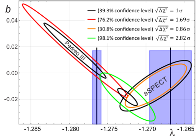
Figure 2: Confidence region for the ratio $\lambda=g_{\text{A}}/g_{\text{V}}$ and the Fierz interference parameter $b$. The results of a correlated $(b,\lambda)$ analysis of the Perkeo III and aSPECT measurements are shown as error ellipses representing specified confidence levels. The combined^(c) result from the two independent data sets suggests a finite value of $b$ with $b^{\text{(c)}}=-0.0181\pm 0.0065$ which deviates by $2.82\sigma$ from the SM (shown by the green error ellipse). For the SM analysis ($b\equiv 0$) of the two measurements, their $\lambda$-values disagree by 3.4 standard deviations (blue vertical bars: $1\sigma$ error).

III Conclusion and Outlook

In this paper, we present a reanalysis of the aSPECT data with an improved tracking of some of the systematic errors. The value $a=-0.10402(82)$ differs only marginally from the one published in [11]. The aSPECT experiment also has sensitivity to $b$. With $b=-0.0098\pm 0.0194$ we demonstrated the extraction of limits on the Fierz interference term from a combined $(b,a)$-analysis of the proton recoil spectrum. The apparent tension to the Perkeo III result [5] based on the SM analysis can be resolved by combining the results of the $(b,\lambda)$ analyses from these two measurements. The finite value for the Fierz interference term of $b^{\text{(c)}}=-0.0184\pm 0.0065$ deviates by $2.82\sigma$ from the SM. The goodness of fit test shows that the $(b,\lambda)$ data from Perkeo III and aSPECT are statistically compatible with the combined result. The upcoming Nab experiment [47] and the next generation instruments like PERC [48, 49] will allow the measurement of decay correlations with strongly improved statistical uncertainties to underpin these findings or to establish that the SM differences are of experimental origin.

References

- [1] S. Baeßler, F. Ayala Guardia, M. Borg, F. Glück, W. Heil, G. Konrad, I. Konorov, R. Muñoz Horta, G. Petzoldt, D. Rich et al., Eur. Phys. J. A 38, 17 (2008).
- [2] F. Glück, S. Baeßler, J. Byrne, M. G. D. van der Grinten, F. J. Hartmann, W. Heil, I. Konorov, G. Petzoldt, Y. Sobolev, and O. Zimmer, Eur. Phys. J. A 23, 135 (2005).
- [3] O. Zimmer, J. Byrne, M. van der Grinten, W. Heil, and F. Glück, Nucl. Instrum. Methods A 440, 548 (2000).
- [4] J. Jackson, S. Treiman, and H. Wyld, Phys. Rev. 106, 517 (1957).
- [5] B. Märkisch et al. (PERKEO III Collaboration), Phys. Rev. Lett. 112, 242501 (2019).
- [6] M.-P. Brown et al. (UCNA Collaboration), Phys. Rev. C 97, 035505 (2018).
- [7] M. Fierz, Z. f. Physik 104, 553 (1937).
- [8] H. Abele, Prog. Part. Nucl. Phys. 60, 1 (2008).
- [9] V. Lobashev and P. Spivak, Nucl. Instrum. Methods A 240, 305 (1985).
- [10] A. Picard et al., Nucl. Instrum. Methods B 63, 345 (1992).
- [11] M. Beck et al., Phys. Rev.C 101, 055506 (2020).
- [12] J. F. Ziegler, M. Ziegler, and J. Biersack, Nucl. lnstrum. Methods A 268, 1818 (2010).
- [13] M. Posselt and J.P. Biersack, Nucl. Instrum. Methods B 64, 706 (1992).
- [14] M. Posselt, Radiat. Effects Def. Solids 130/131, 87 (1994).
- [15] P.Dumas, J.P. Dubarry-Barbe, D. Riviere, Y.Levy, and J. Corset,Journal de Physique Colloque 44, C10-205 (1983) .
- [16] K. Nordlund, F. Djurabekova, and G. Hobler, Phys. Rev. B 94 ,214109 (2016) .
- [17] K. Nordlund, Comput. Mater. Sci. 3, 448 (1995).
- [18] M. Popp, R. Hartmann, H. Soltau, L. Strüder, N. Meidinger, P. Holl, N. Krause, and C. von Zanthier, Nucl. Instrum. Methods A 439, 567 (2000).
- [19] W. Pilz, J.V. Borany, R. Grötzschel, W. Jiang, M. Posselt, B. Schmidt, Nucl. Instrum. Methods A 419, 137 (1998).
- [20] G. Hobler, Nucl. Instrum. Methods B 115, 323 (1996).
- [21] J.A. Phillips, Phys. Rev. 97, 404 (1955).
- [22] P.Lechner, A.Pahlke, and H.Soltau, X-Ray Spectrom. 33, 256 (2004).
- [23] F. Glück, Phys. Rev. D47, 2840 (1993).
- [24] F. Glück , Radiative corrections to neutron and nuclear -decays: a serious kinematics problem in the literature, arXiv:2205.05042v1 (2022).
- [25] D.H. Wilkinson, Nucl. Phys. A 377, 474 (1982) and references therein.
- [26] S. Weinberg, Phys. Rev. 115, 481 (1959) .
- [27] F. Glück, I. Joo, and J. Last, Nucl. Phys. A 593, 125 (1995).
- [28] M. González-Alonso, and O. Naviliat-Cuncic, Phys. Rev. C 94, 035503 (2016).
- [29] J. Beringer et al. (Particle Data Group), Phys. Rev. D 86, 010001 (2012).
- [30] R.L. Workman et al. (Particle Data Group), Prog. Theor. Exp. Phys. 2022, 083C01 (2022) and 2023 update .
- [31] H. Saul, C. Roick, H. Abele, H. Mest, M. Klopf, A. K. Petukhov, T. Soldner, X. Wang, D. Werder, and B. Märkisch, Phys. Rev. Lett.125, 112501 (2020).
- [32] M.T. Hassan et al., Phys. Rev. C 103, 045502 (2021).
- [33] F.E. Wietfeldt at al., Recoil-Order and Radiative Corrections to the aCORN Experiment, arXiv: 2306.15042v1 (2023) .
- [34] X. Sun et al., Phys. Rev. C 101, 035503 (2020) .
- [35] D. Mund, B. Märkisch, M. Deissenroth, J. Krempel, M. Schumann, H. Abele, A.K. Petukhov, and T. Soldner, Phys. Rev. Lett. 110, 172502 (2013).
- [36] O. Erten, and C.V. Deutsch, Combination of multivariate Gaussian distributions through error ellipses. Geostatistics Lessons (2020).
- [37] N. Orsini, R. Bellocco, and S. Greenland, The Stata Journal 6 (1), 40 (2006).
- [38] N.M. Blachman, On combining target-location ellipses, IEEE Trans. Aerospace and Electronic Systems25(2), 284 (1989).
- [39] T. Bhattacharya, V. Cirigliano, S.D. Cohen, A. Filipuzzi, M. González-Alonso, M.L. Graesser, R. Gupta, and H.-W. Lin, Phys. Rev D 85, 054512 (2012).
- [40] M. Bychkov et al., Phys. Rev. Lett. 103, 051802 (2009).
- [41] A. Falkowski, M. González-Alonso, and O. Naviliat-Cuncic, J. High Energ. Phys. 2021, 126 (2021).
- [42] R. Gupta, Y.-C. Jang, B.Yoon, H.-W. Lin,V.Cirigliano, and T. Bhattacharya, Phys. Rev. D 98, 034503 (2018).
- [43] A. Czarnecki, W.J. Marciano, and A. Sirlin, Phys. Rev. Lett. D 100, 073008 (2019).
- [44] A.N. Ivanov, R. Höllwieser, N.I. Troitskaya, M. Wellenzahn, and Ya.A. Berdnikov, Phys. Rev. C 98, 035503 (2018) .
- [45] M.T. Burkey et al., Phys. Rev. Lett. 128 , 202502 (2022) .
- [46] V. Cirigliano, M. González-Alonso, and M. L. Graesser, J. High Energ. Phys. 2013, 46 (2013)
- [47] J. Fry et al., EPJ Web Conf. 219, 04002 (2019).
- [48] D. Dubbers, H. Abele, S. Baeßler, B. Märkisch, M. Schumann, T. Soldner, and O. Zimmer, Nucl. Instrum. Methods A 596, 238 (2008).
- [49] G. Konrad et al. (PERC Collaboration), J. Phys. 340, 012048 (2012).