Growth factors of orthogonal matrices and local behavior of Gaussian elimination with partial and complete pivoting

Abstract

Gaussian elimination (GE) is the most used dense linear solver. Error analysis of GE with selected pivoting strategies on well-conditioned systems can focus on studying the behavior of growth factors. Although exponential growth is possible with GE with partial pivoting (GEPP), growth tends to stay much smaller in practice. Support for this behavior was provided last year by Huang and Tikhomirov’s average-case analysis of GEPP, which showed GEPP growth factors stay at most polynomial with very high probability when using small Gaussian perturbations. GE with complete pivoting (GECP) has also seen a lot of recent interest, with improvements to lower bounds on worst-case GECP growth provided by Edelman and Urschel earlier this year. We are interested in studying how GEPP and GECP behave on the same linear systems as well as studying large growth on particular subclasses of matrices, including orthogonal matrices. We will also study systems when GECP leads to larger growth than GEPP, which will lead to new empirical lower bounds on how much worse GECP can behave compared to GEPP in terms of growth. We also present an empirical study on a family of exponential GEPP growth matrices whose polynomial behavior in small neighborhoods limits to the initial GECP growth factor.

15A23, 65G50, 65F99

1 Introduction and motivations

Gaussian elimination (GE) remains the most used dense linear solver of a linear system $A{\mathbf{x}}={\mathbf{b}}$ for $A\in\mathbb{R}^{n\times n}$. In addition to a chosen pivoting strategy, GE transforms the initial matrix $A=A^{(1)}$ into an upper triangular matrix $U=A^{(n)}$ by iteratively using the leading row of the untriangularized system and and its first entry (i.e., the pivot) to zero out below the main diagonal, forming $A^{(k)}$ with 0’s below the $k-1$ diagonal entry for each $k=2$ to $n$. This results in the final factorization $PAQ=LU$ using $\frac{2}{3}n^{3}(1+o(1))$ FLOPs, where $L$ is unipotent lower triangular and $P,Q$ are permutation matrices that account for the necessary row and column swaps mandated by the chosen pivoting strategy. This work will focus on GE with no pivoting (GENP), partial pivoting (GEPP), and complete pivoting (GECP). (See Appendix A for a definition of GE and each pivoting scheme.)

Understanding the behavior of GE under floating-point arithmetic has been an ongoing focus of numerical analysis for over 60 years. Early work by Wilkinson in [30], which led to the start of error analysis, established studying the relative errors of computed solutions $\hat{{\mathbf{x}}}$ to $A{\mathbf{x}}={\mathbf{b}}$ through the bound

(1) $$\frac{\|{\mathbf{x}}-\hat{{\mathbf{x}}}\|_{\infty}}{\|{\mathbf{x}}\|_{\infty}}\leq 4n^{2}\epsilon_{\operatorname{machine}}\kappa_{\infty}(A)\rho(A),$$

where $\epsilon=\epsilon_{\operatorname{machine}}$ denotes the machine epsilon (see Appendix A), $\kappa_{\infty}(A)=\|A\|_{\infty}\|A^{-1}\|_{\infty}$ the $\infty$-condition number and

(2) $$\rho(A)=\frac{\displaystyle\|L\|_{\max}\max_{k}\|A^{(k)}\|_{\max}}{\|A\|_{\max}}$$

is the growth factor. In well-conditioned linear systems, error analysis of GE can then be reduced to analysis of the growth factor through (1).

Understanding worst-case bounds on $\rho$ using different pivoting strategies has been a continued area of research since Wilkinson’s initial analysis. We will focus on growth factors using GEPP and GECP on real matrices. For nonsingular matrices $\operatorname{GL}_{n}(\mathbb{R})$, we can define the maps

(3) $$\rho^{\operatorname{GEPP}}: \operatorname{GL}_{n}(\mathbb{R})\to[1,a_{n}]$$

(4) $$\rho^{\operatorname{GECP}}: \operatorname{GL}_{n}(\mathbb{R})\to[1,b_{n}]$$

Finding the worst-case bounds for each growth factor is equivalent then to find the optimal upper bounds $a_{n}$ and $b_{n}$ for each range and pivoting strategy. For $\mathcal{S}\subset\operatorname{GL}_{n}(\mathbb{R})$, define

(5) $$g(\mathcal{S}):=\max_{A\in\mathcal{S}}\rho(A),$$

and let $g_{n}=g(\operatorname{GL}_{n}(\mathbb{R}))$. So optimal choices for $a_{n}$ and $b_{n}$ are then necessarily the increasing sequences $a_{n}=g_{n}^{\operatorname{GEPP}}$ and $b_{n}=g_{n}^{\operatorname{GECP}}$.

Worst-case behavior on GEPP has been completely understood since Wilkinson’s initial foray [30], where he established

(6) $$g_{n}^{\operatorname{GEPP}}=2^{n-1}.$$

Worst-case behavior of GECP, however, remains elusive. This exact value can be established so far only for $n\leq 4$ (see [5, 6, 11]). Using Hadamard’s inequality in the same work, Wilkinson established the upper bound

(7) $$g^{\operatorname{GECP}}_{n}\leq(n\cdot 2\cdot 3^{1/2}\cdots n^{1/(n-1)})^{1/2}\leq 2\cdot n^{\ln n/4+1/2}.$$

This bound is believed to be very pessimistic. For a long time a conjecture (of apocryphal origins) ventured the bound $g_{n}^{\operatorname{GECP}}\leq n$. This would essentially match the trivial lower bounds for $g_{n}^{\operatorname{GECP}}$ of $(n+1)/2$ for any $n$ and $n$ whenever a Hadamard matrix exists (see [16]). This conjectured upper bound maintained the popular vote for three decades until Gould found a “counterexample” using floating-point arithmetic for $n=13$ with a GECP growth factor of 13.0205 [14]. Edelman confirmed a true counterexample in exact arithmetic shortly after by adjusting one entry of Gould’s rationalized matrix by $10^{-7}$ [9]. Since then, not a lot of significant progress has been made on improving Wilkinson’s original pessimistic upper bound. The lower bound of $n$, however, has been significantly improved just this year (another 30 years later) by Edelman and Urschel, who established $g_{n}^{\operatorname{GECP}}\geq 1.0045n$ for all $n\geq 11$ and $g_{n}^{\operatorname{GECP}}\gtrsim 2.525n$, and they further conjectured $g_{n}^{\operatorname{GECP}}=\omega(n)$ [11]. Meanwhile, the previous upper bound of $n$ on GECP growth can now be conjectured to still hold for Hadamard matrices (if they exist) or potentially orthogonal matrices (which contain scaled Hadamard matrices). The question of maximal growth on Hadamard matrices has its own rich history and active research (e.g., [7, 12, 19, 32]).

Additionally, we are interested in how GEPP and GECP act on the same linear systems rather than just their worst-case behavior separately. That is, we are interested in establishing optimal bounds on the range of the map

(8) $$\rho^{\operatorname{GEPP}}-\rho^{\operatorname{GECP}}: \operatorname{GL}_{n}(\mathbb{R})\to[-c_{n},d_{n}],.$$

Studying the bounds $c_{n}$ and $d_{n}$ can then establish how much worse one pivoting strategy can behave relative to the other.

Not a lot of research has studied the behavior between these pivoting schemes used on the same linear systems. It’s clear $0\in[-c_{n},d_{n}]$ since if no pivoting is needed on a matrix using GECP, then that would also be the case for GEPP, so both growth factors must align. Trivial bounds can be put on $c_{n}$ and $d_{n}$ using $a_{n}$ and $b_{n}$: $c_{n}\leq b_{n}-1$ and $d_{n}\leq a_{n}-1=2^{n-1}-1$. For $d_{n}$, that measures how much worse GEPP can behave relative to GECP, this can be answered exactly: it is as bad as it can get. In other words, the trivial upper bound,

(9) $$d_{n}=2^{n-1}-1,$$

is the optimal choice for $d_{n}$ for all $n$. This is established by noting the matrix $\tilde{A}_{n}$ formed using Wilkinson’s worst-case bound matrix $A_{n}$ (see (18)) with its last column multiplied by 2 attains the trivial upper bound. Multiplying the last column by 2 does not change the GEPP growth factor from that for $A_{n}$ (see Theorem 3.7), so $\rho^{\operatorname{GEPP}}(\tilde{A}_{n})=\rho^{\operatorname{GEPP}}(A_{n})=2^{n-1}$, but it now reduces the GECP growth factor to the minimal value $\rho^{\operatorname{GECP}}(\tilde{A}_{n})=1$: every GECP step starts with a column swap with the last column, which is always a $\pm 2$ constant multiple of an all 1’s vector while the prior columns of the $(n-k+1)\times(n-k+1)$ untriangularized block match those of $A_{n-k+1}$; this establishes no entry ever exceeds $2=\|\tilde{A}_{n}\|_{\max}$ at any GECP step. For example, $\tilde{A}_{4}$ has the final GECP factorization

(10) $$\begin{bmatrix}1&&&2\\ -1&1&&2\\ -1&-1&1&2\\ -1&-1&-1&2\end{bmatrix}\begin{bmatrix}&1\\ &&1\\ &&&1\\ 1\end{bmatrix}=\begin{bmatrix}1\\ 1&1\\ 1&1&1\\ 1&1&1&1\end{bmatrix}\begin{bmatrix}2&1\\ &-2&1\\ &&-2&1\\ &&&-2\end{bmatrix}$$

so that $\rho^{\operatorname{GECP}}(\tilde{A}_{4})=1$.

Finding an optimal value of $c_{n}$ proves more interesting; after all, the trivial upper bound uses the still elusive constant $b_{n}=g_{n}^{\operatorname{GECP}}$. The general consensus is that GECP should lead to higher accuracy than GEPP and hence smaller growth, so a common assumption is that $\rho^{\operatorname{GEPP}}\geq\rho^{\operatorname{GECP}}$. This inequality can easily be shown to hold for $n=2$ (so the optimal interval is $[-c_{2},d_{2}]=[0,1]$), but this fails starting at $n=3$. This can be exhibited by

(11) $$B_{3}=\begin{bmatrix}1/2&0&1/2\\ 1/2&1&1\\ 1/2&-1&1\end{bmatrix},$$

which has $\rho^{\operatorname{GEPP}}(B_{3})=1$ and $\rho^{\operatorname{GECP}}(B_{3})=2$. Hence, after similarly noting $c_{n}$ is a monotonically increasing sequence, this establishes $c_{n}\geq 1$ for all $n\geq 3$. Natural questions arise out of this brief exploration. How large does $c_{n}$ get? How far is $c_{n}$ from the trivial bound $b_{n}-1$? How often does GEPP result in smaller growth factors than GECP? How far away can the GEPP growth factor be from the initial GECP growth factor in a small neighborhood?

1.1 Outline of paper

This paper uses both theoretical and numerical approaches to explore the behavior of GEPP and GECP on $\operatorname{GL}_{n}(\mathbb{R})$ and the orthogonal matrices, $\operatorname{O}(n)$. In order to gain a richer understanding of $b_{n}$ and $c_{n}$ as well as to get a foothold to approach some of these above questions, we will study the corresponding constants (now also including $a_{n}$ and $d_{n}$) when restricting the growth factor maps to $\operatorname{O}(n)$. Studying growth factors on more structured systems has proven fruitful. For instance, the behavior of GENP, GEPP and GE with rook pivoting (GERP) is now completely understood when using $\bigotimes^{n}\operatorname{SO}(2)$ [21].

Although GE should not be a first choice for solving orthogonal linear systems, there are situations when applying GE to orthogonal matrices makes sense. For example, Barlow needed to understand the effect of GEPP on orthogonal matrices to carry out error analysis of bidiagonal reduction [2]. This led to Barlow and Zha’s analysis using GEPP on orthogonal matrices, which they showed maximized a different $L^{2}$-growth factor, $\rho_{2}$ (see (21)). Additionally, while original studies of random growth factors tended to focus on ensembles with independent and identically distributed (iid) entries, many authors noted and explored the potential that orthogonal matrices can produce larger growth factors. For example, the original lower bounds of $(n+1)/2$ and $n$ for $g_{n}^{\operatorname{GECP}}$ came from properties of particular orthogonal ensembles [5, 16, 17, 25]. Hence, orthogonal matrices remain a rich source of study for potential large growth factors.

Necessary background and notation for what follows is included in Appendix A. In Section 2, we give a brief overview of the interaction of GEPP and GECP growth for small $n$. We also provide summary statistics for random growth samples using both $\operatorname{Haar}\operatorname{O}(n)$ and $\operatorname{Ginibre}(n,n)$, which align with previous results in the literature (e.g., [25]). In Section 3, we revisit the orthogonal matrix $Q_{n}$, which was originally studied by Barlow and Zha in [3]. In Proposition 3.1, we provide explicit intermediate GEPP forms for $Q_{n}$, which then yields asymptotic GEPP growth $\rho^{\operatorname{GEPP}}(Q_{n})=(2^{n-1}/\sqrt{3})(1+o(1))$ in Corollary 3.3. This model then provides an improved worst-case bound $g^{\operatorname{GEPP}}(\operatorname{O}(n))=c2^{n-1}(1+o(1))$ for some $c\in[\frac{1}{\sqrt{3}},1)$ in Theorem 3.11. Proofs for results in Section 3 are found in Appendix B.

In Section 4, we explore properties of orthogonal perturbations of linear systems. This study is analogous to the study of additive perturbations by Gaussian matrices, which was the basis for the smoothed analysis of GENP carried out by Sankar, Speilman, and Teng as well as that of GEPP carried out by Sankar in his dissertation and the very recent average-case analysis of GEPP work of Huang and Tikhomirov [18, 23, 22]. In these prior works, both the $L^{2}$-condition number, $\kappa_{2}$, and growth factors are studied under small additive perturbations by Gaussian matrices. Studying small multiplicative orthogonal perturbations on linear systems, which preserves $\kappa_{2}$, enables study only of the growth factors themselves.

In Section 4.2, we focus on addressing how much worse can GECP behave compared to GEPP in terms of growth. We employ random search paths generated through small perturbations to introduce new estimates for lower bounds for maximal GECP-GEPP growth differences for both $\operatorname{GL}_{n}(\mathbb{R})$ and $\operatorname{O}(n)$ (see Figure 4). Section 4.3 explores the local GEPP and GECP growth behavior for linear systems that exhibit extreme GEPP-GECP growth differences. With one exception, growth remains stable under the pivoting strategy that has minimal initial growth, while the larger growth models has local behavior progressively concentrate near the smaller initial growth. For particular exponential GEPP growth models, our study provides an empirical qualification for the Huang and Tikhomirov result that at most polynomial local growth will be encountered with high probability using GEPP. For our models, we then show the polynomial growth that is encountered locally limits to the initial GECP growth factor.

2 Growth factors for small $n$

While $g_{n}^{\operatorname{GEPP}}$ has been known since Wilkinson’s original analysis, much less is known about $g_{n}^{\operatorname{GECP}}$. The only known exact values of $g_{n}^{\operatorname{GECP}}$ are for $n=1$, 2, 3, $4$, which take the values exactly 1, 2, 2.25, 4, respectively, while there is a bound $g_{5}^{\operatorname{GECP}}\leq 4\frac{17}{18}$. Best known lower bounds for other small $n$ are found in [11]. The known constants $g_{n}^{\operatorname{GECP}}$ all carry over for $g^{\operatorname{GECP}}(\operatorname{O}(n))$ since an orthogonal matrix can be constructed to match each upper bound: a Hadamard matrix can be scaled to be orthogonal to meet each of the $n=1$, 2, 4 bounds, while the standard matrix (used in [5, 6]) that attains $g_{3}^{\operatorname{GECP}}=2.25$,

(12) $$C=\begin{bmatrix}1&1&1/2\\ -1&1/2&1\\ 1/2&-1&1\end{bmatrix}.$$

is also a scalar multiple of an orthogonal matrix, $\frac{2}{3}C\in\operatorname{O}(3)$.

To better understand the overall relationship between GEPP and GECP growth factors used on the same linear systems, we will first explore this question when restricting our study to $\operatorname{O}(n)$. This is trivial for $n=2$ since both growth factors necessarily align when working with $\operatorname{O}(n)$.

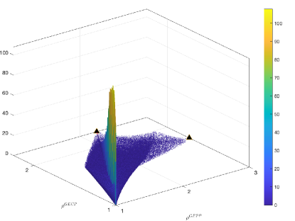
(a) Front view

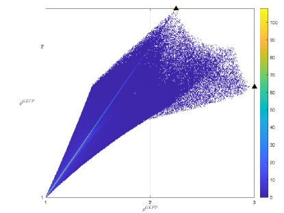
(b) Top view

Figure 1: Normalized histogram of $512\times 512$ grid for each pair of $\rho^{\operatorname{GEPP}}$ and $\rho^{\operatorname{GECP}}$ using $10^{6}$ $\operatorname{Haar}(\operatorname{O}(3))$ samples, with marks at $(2.25,2.25)$ and $(3,\sqrt{3})$ corresponding to (12) and (13).

For $n=3$, this is no longer the case. Figure 1 shows a top view normalized histogram (using a $512\times 512$ grid) of pairings $(\rho^{\operatorname{GEPP}},\rho^{\operatorname{GECP}})$ for $10^{6}$ matrices sampled from $\operatorname{Haar}(\operatorname{O}(3))$. Marks are also included on Figure 1 for (12), which is CP and hence also PP so has $\rho^{\operatorname{GEPP}}(B_{2})=\rho^{\operatorname{GECP}}(B_{2})=2.25$, along with for

(13) $$Q_{3}=\begin{bmatrix}1&0&2\\ -1&1&1\\ -1&-1&1\end{bmatrix}\begin{bmatrix}3\\ &2\\ &&6\end{bmatrix}^{-1/2},$$

which has $\rho^{\operatorname{GEPP}}(Q_{3})=3$ and $\rho^{\operatorname{GECP}}(Q_{3})=\sqrt{3}$. $Q_{3}$ is an instance of a particular family of orthogonal matrices that will be studied more extensively in Section 3.

Figure 1 exhibits huge concentration for the pairs of growth factors along the line $\rho^{\operatorname{GEPP}}=\rho^{\operatorname{GECP}}$. Tables 1 and 2 include summary statistics for $10^{6}$ random samples for $\operatorname{Haar}\operatorname{O}(n)$ and $\operatorname{Ginibre}(n,n)$ for $n=2:20,50,100$. In line with Figures 1 and 1, over 65% of the samples were concentrated within $.05$ of the line $\rho^{\operatorname{GEPP}}=\rho^{\operatorname{GECP}}$. The concentration along the line $\rho^{\operatorname{GEPP}}=\rho^{\operatorname{GECP}}$ for $n=3$ is more prominent if using $A\sim\operatorname{Ginibre}(n,n)$ (see Table 2), with over 70% of samples near this line.

Using the estimates from Tables 1 and 2, we can empirically address the question on how often does GECP growth exceed GEPP growth for each random ensemble. Both ensembles have GEPP and GECP growth factors that have a positive fraction lie above the line $\rho^{\operatorname{GECP}}=\rho^{\operatorname{GEPP}}$, i.e, a positive portion satisfies $\mathbb{P}(\rho^{\operatorname{GECP}}>\rho^{\operatorname{GEPP}})$, with the sample proportion starting at about 13% for $\operatorname{Haar}\operatorname{O}(3)$ and 1.4% for $\operatorname{Ginibre}(3,3)$. As $n$ increases, this decreases for both ensembles, with $\operatorname{Ginibre}(n,n)$ in particular seeing this proportion decrease approximately exponentially fast, with $\mathbb{P}(\rho^{\operatorname{GECP}}>\rho^{\operatorname{GEPP}})\approx e^{-\alpha n}$ where $\alpha\approx 1/3$ for $\operatorname{GL}_{n}(\mathbb{R})$. $\operatorname{O}(n)$ also has this proportion vanish, but at a slower rate, with $\mathbb{P}(\rho^{\operatorname{GECP}}>\rho^{\operatorname{GEPP}})=\mathcal{O}(n^{-2})$ empirically.

Remark 2.1.

Figure 2 plots each average growth factor for each set of samples using $\operatorname{Haar}(\operatorname{O}(n))$ and $\operatorname{Ginibre}(n,n)$. Results are consistent with other studies, such as the first average-case analysis of GE carried out by Trefethen and Schreiber in 1990 [25]. In their empirical studies, they conjectured $\operatorname{Ginibre}(n,n)$ has asymptotic normalized average growth of $n^{2/3}$ for GEPP and $n^{1/2}$ for GECP for $n$ up to about 1000, while they also further conjectured both normalized average growth rates are $\mathcal{O}(n^{1/2})$ asymptotically. Higham, Higham and Pranesh establish that $\rho(Q)\gtrsim n/(4\log n)$ for $Q\sim\operatorname{Haar}\operatorname{O}(n)$ using any pivoting strategy, which again aligns with Figures 2 and 1 [17].

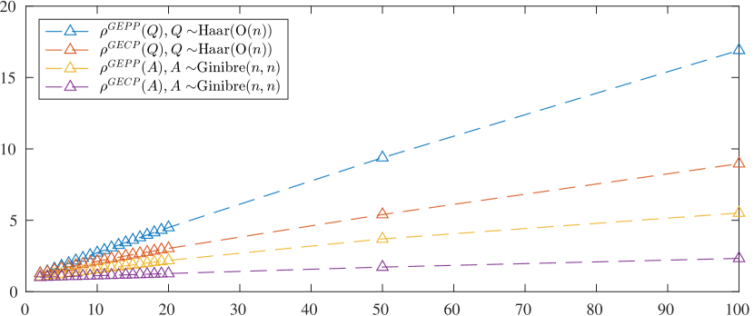
Figure 2: Plot of the average computed growth factors for $10^{6}$ samples of $\operatorname{Haar}\operatorname{O}(n)$ and $\operatorname{Ginibre}(n,n)$ for $n=2:20,50,100$.

	$\rho^{\operatorname{GEPP}}$			$\rho^{\operatorname{GECP}}$			$\approx\mathbb{P}(\rho^{\operatorname{GEPP}}(<,=,>)\rho^{\operatorname{GECP}})$
$n$	Median	$\bar{x}$	$s$	Median	$\bar{x}$	$s$	$<$	$=$	$>$
2	1.1714	1.2730	0.2765	1.1714	1.2730	0.2765	-	1	-
3	1.3571	1.4110	0.2847	1.3557	1.3795	0.2223	0.1297	0.6536	0.2167
4	1.5372	1.6061	0.3381	1.4949	1.5200	0.2256	0.1696	0.4355	0.3949
5	1.7191	1.7917	0.3857	1.6040	1.6308	0.2244	0.1545	0.3058	0.5397
6	1.9017	1.9807	0.4357	1.7085	1.7362	0.2330	0.1290	0.2216	0.6494
7	2.0828	2.1678	0.4832	1.8098	1.8371	0.2429	0.1048	0.1652	0.7300
8	2.2606	2.3521	0.5293	1.9085	1.9355	0.2537	0.0856	0.1245	0.7899
9	2.4372	2.5382	0.5780	2.0072	2.0336	0.2650	0.0711	0.0955	0.8335
10	2.6118	2.7212	0.6238	2.1032	2.1295	0.2762	0.0593	0.0743	0.8664
11	2.7858	2.9042	0.6707	2.1984	2.2242	0.2867	0.0497	0.0591	0.8912
12	2.9570	3.0837	0.7150	2.2918	2.3173	0.2972	0.0428	0.0475	0.9097
13	3.1283	3.2633	0.7598	2.3839	2.4097	0.3077	0.0370	0.0382	0.9248
14	3.2987	3.4430	0.8048	2.4754	2.5013	0.3185	0.0316	0.0317	0.9368
15	3.4679	3.6196	0.8473	2.5652	2.5909	0.3280	0.0278	0.0260	0.9461
16	3.6355	3.7957	0.8919	2.6546	2.6802	0.3376	0.0240	0.0218	0.9541
17	3.8013	3.9707	0.9333	2.7430	2.7694	0.3480	0.0214	0.0184	0.9603
18	3.9709	4.1474	0.9774	2.8303	2.8569	0.3572	0.0186	0.0155	0.9660
19	4.1331	4.3168	1.0156	2.9156	2.9424	0.3672	0.0166	0.0135	0.9698
20	4.2981	4.4928	1.0625	3.0020	3.0285	0.3764	0.0149	0.0114	0.9737
50	8.9687	9.3818	2.2129	5.3573	5.4007	0.6380	0.0016	0.0007	0.9978
100	16.156	16.9045	3.9513	8.8896	8.9626	1.0245	0.0003	0.0001	0.9996

Table 1: Summary statistics for computed $\rho^{\operatorname{GEPP}}(A)$ and $\rho^{\operatorname{GECP}}(A)$ using $10^{6}$ samples $A\sim\operatorname{Haar}\operatorname{O}(n)$

	$\rho^{\operatorname{GEPP}}$			$\rho^{\operatorname{GECP}}$			$\approx\mathbb{P}(\rho^{\operatorname{GEPP}}(<,=,>)\rho^{\operatorname{GECP}})$
$n$	Median	$\bar{x}$	$s$	Median	$\bar{x}$	$s$	$<$	$=$	$>$
2	1.0000	1.0438	0.1247	1.0000	1.0112	0.0598	-	0.871459	0.128541
3	1.0000	1.0974	0.1811	1.0000	1.0270	0.0883	0.0139	0.7060	0.2802
4	1.0480	1.1549	0.2235	1.0000	1.0415	0.1038	0.0255	0.5494	0.4250
5	1.1315	1.2167	0.2602	1.0000	1.0558	0.1153	0.0317	0.4144	0.5539
6	1.2076	1.2804	0.2905	1.0000	1.0694	0.1236	0.0326	0.3067	0.6607
7	1.2789	1.3466	0.3184	1.0000	1.0829	0.1302	0.0303	0.2214	0.7483
8	1.3463	1.4131	0.3422	1.0220	1.0959	0.1354	0.0260	0.1572	0.8168
9	1.4136	1.4811	0.3642	1.0491	1.1094	0.1401	0.0209	0.1104	0.8687
10	1.4803	1.5489	0.3839	1.0735	1.1231	0.1445	0.0165	0.0766	0.9070
11	1.5447	1.6160	0.4026	1.0962	1.1370	0.1482	0.0124	0.0532	0.9345
12	1.6090	1.6827	0.4197	1.1175	1.1511	0.1515	0.0095	0.0359	0.9546
13	1.6723	1.7485	0.4358	1.1367	1.1650	0.1541	0.0068	0.0251	0.9682
14	1.7359	1.8138	0.4511	1.1554	1.1790	0.1564	0.0049	0.0169	0.9782
15	1.7975	1.8782	0.4668	1.1733	1.1936	0.1591	0.0035	0.0120	0.9846
16	1.8593	1.9419	0.4800	1.1912	1.2086	0.1612	0.0024	0.0082	0.9893
17	1.9200	2.0048	0.4938	1.2081	1.2233	0.1629	0.0017	0.0059	0.9924
18	1.9802	2.0666	0.5058	1.2252	1.2385	0.1646	0.0012	0.0041	0.9947
19	2.0391	2.1273	0.5182	1.2422	1.2536	0.1661	0.0009	0.0029	0.9963
20	2.0983	2.1889	0.5313	1.2584	1.2692	0.1673	0.0005	0.0020	0.9974
50	3.5612	3.6942	0.7950	1.7125	1.7207	0.1924	-	-	1
100	5.3353	5.5101	1.0603	2.3197	2.3295	0.2283	-	-	1

Table 2: Summary statistics for computed $\rho^{\operatorname{GEPP}}(A)$ and $\rho^{\operatorname{GECP}}(A)$ using $10^{6}$ samples $A\sim\operatorname{Ginibre}(n,n)$

Remark 2.2.

One property that is not obvious from Figure 1 is how far away from the initial GECP growth factor are the GEPP growth factors for neighbors of an orthogonal matrix. This will be viewed much more extensively in Section 4.

Since $\operatorname{O}(n)$ is compact, then the image for the map $Q\mapsto(\rho^{\operatorname{GEPP}}(Q),\rho^{\operatorname{GECP}}(Q))$ will be compact. Establishing exactly what that image will be is also interesting in itself. For $n=3$, sampling $10^{6}$ $\operatorname{Haar}\operatorname{O}(3)$ matrices gives a good idea of what that image looks like (see Figure 1). Moreover, other attributes of this map for $n=3$ can be explicitly analyzed by utilizing the factorization of $\operatorname{O}(3)$ as the product of three Givens rotations, $G(\theta_{3},2,3)G(\theta_{2},1,3)G(\theta_{1},1,2)$. Using this approach, for instance, one can establish $g^{\operatorname{GEPP}}(\operatorname{O}(3))=3$, which is achieved by $Q_{3}$.

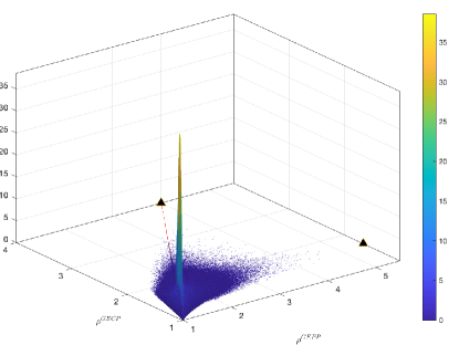
(a) Front view

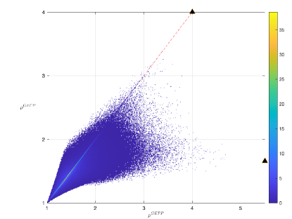
(b) Top view

Figure 3: Normalized histogram using $512\times 512$ grid of each pair of $\rho^{\operatorname{GEPP}}$ and $\rho^{\operatorname{GECP}}$ using $10^{6}$ $\operatorname{Haar}(\operatorname{O}(4))$ samples, with marks at the points (4,4) (for a scaled Hadamard matrix) and $(11/2,\sqrt{11}/2)$ associated to (17).

This approach is untenable in general as $\dim\operatorname{O}(n)={n(n-1)}/2$ provides the minimal number of Givens rotations that would be needed. For $n=4$, uniform sampling is less effective at estimating this image, as seen in Figure 3. In particular, while samples were found near $(3,\sqrt{3})$ in Figure 1, no sample was close to the point $(11/2,\sqrt{11}/2)\approx(5.5,1.658312395)$ associated with the matrix

(17) $$Q_{4}=\begin{bmatrix}1&-1&0&4\\ -1&5&0&2\\ -1&-3&1&1\\ -1&-3&-1&1\end{bmatrix}\begin{bmatrix}4\\ &44\\ &&2\\ &&&22\end{bmatrix}^{-1/2},$$

which is again from the special class of orthogonal matrices that will be studied in Section 3. In fact, no GEPP growth factor exceeded 4.6956 in the $10^{6}$ samples, while only 56 samples (i.e., 0.0056%) had a GEPP growth factor exceed 4. Similarly, no uniformly sampled points had GECP growth factor larger than 3.3913, far from the maximal GECP growth of 4 attainable by any scaled Hadamard matrix.

From Figures 1 and 3, it appears for $\operatorname{O}(n)$ that the GECP growth factors are much more limited in how much larger they can be than the GEPP growth factors compared to the general case. In particular, while $B_{3}$ from (11) had a difference of 1, attaining the point $(1,2)$, no point for $\operatorname{O}(3)$ nor $\operatorname{O}(4)$ exhibits a difference in coordinates farther than about 0.2988 for $n=3$ and 0.5852 for $n=4$. Similarly, the extreme points associated to $a_{n}$, for large GEPP growth, as well as $d_{n}$, for how much larger GEPP growth factors can be than the GECP growth factors, appears closest to the point for the constructed matrices we will explore in Section 3. Section 4 will revisit each of these constants both for the $\operatorname{O}(n)$ and $\operatorname{GL}_{n}(\mathbb{R})$ cases.

3 Large GEPP growth factors for $\operatorname{O}(n)$

In this section, we present an explicit construction of an orthogonal matrix that attains exponential GEPP growth. We use this model to present improved estimates for the worst-case GEPP growth and worst-case GEPP-GECP growth difference for orthogonal matrices. Proofs for results in this section are are found in Appendix B.

3.1 Exponential orthogonal growth model, $Q_{n}$

We are interested in establishing how large a GEPP growth factor can be on $\operatorname{O}(n)$. A trivial upper bound is $2^{n-1}$, the established maximal GEPP growth for any matrix. In [31, pg. 202], Wilkinson constructed a matrix whose growth attains this upper bound, which takes the form

(18) $$A_{n}={\mathbf{I}}_{n}-\sum_{i>j}{\mathbf{E}}_{ij}+\sum_{i=1}^{n-1}{\mathbf{E}}_{in}$$

and has GENP and also GEPP factorization $A_{n}=L_{n}U_{n}$, where

(19) $$L_{n} ={\mathbf{I}}_{n}-\sum_{i>j}{\mathbf{E}}_{ij}\quad\mbox{and}\quad U_{n}={\mathbf{I}}_{n}-{\mathbf{E}}_{nn}+\sum_{i=1}^{n}2^{i-1}{\mathbf{E}}_{in}.$$

No pivots would be needed at any GEPP step, so the largest growth is easily seen to be encountered in the final pivot, $U_{nn}=2^{n-1}$. For example,

(20) $$A_{4}=\begin{bmatrix}1&&&1\\ -1&1&&1\\ -1&-1&1&1\\ -1&-1&-1&1\end{bmatrix}=\begin{bmatrix}1&&&\\ -1&1&&\\ -1&-1&1&\\ -1&-1&-1&1\end{bmatrix}\begin{bmatrix}1&&&1\\ &1&&2\\ &&1&4\\ &&&8\end{bmatrix}=L_{4}U_{4},$$

has $\rho^{\operatorname{GEPP}}(A_{4})=\rho^{\operatorname{GENP}}(A_{4})=2^{3}=8$.

A perhaps natural candidate for large orthogonal growth could be $Q_{n}$, the orthogonal QR factor for $A_{n}$ One can compute $Q=Q_{4}$ in exact arithmetic (for example, applying Gram-Schmidt to the columns of $L_{4}$), which produces (17). A straightforward check verifies $\rho^{\operatorname{GEPP}}(Q_{4})=5.5$, which is more than 20% larger than any of the previous $10^{6}$ $\operatorname{Haar}\operatorname{O}(4)$ samples encountered from Section 2.

One observation, which will be formally established in Lemma 3.4, is that we would get the exact same orthogonal QR factor if we applied QR directly to $L_{n}$ instead of $A_{n}$. So the assumption that we found large orthogonal growth factor because we started with a matrix with a large growth factor goes unfounded: $L_{n}$ is lower triangular and so has the minimal GEPP growth factor of 1. Regardless, we can now study $Q_{n}$, the orthogonal QR factors of $L_{n}$, to now establish a better bound for $g(\operatorname{O}(n))$.

This exact orthogonal matrix was studied extensively by Barlow and Zha in [3] with the goal of maximizing a different $L^{2}$-growth factor, defined by

(21) $$\rho_{2}(A):=\frac{\displaystyle\max_{k}\|A^{(k)}\|_{2}}{\|A\|_{2}}.$$

The maximizing property follows from orthogonal invariance of the $L^{2}$-norm, which establishes the orthogonal QR factor has larger $\rho_{2}$ value: since $(QR)^{(k)}=[L^{(k)}]^{-1}QR=Q^{(k)}R$ (by Lemma 3.4), then

(22) $$\rho_{2}(QR)\leq\max_{k}\|[L^{(k)}]^{-1}\|_{2}=\rho_{2}(Q).$$

Since $\|A^{-1}\|_{2}=\sigma_{\min}(A)^{-1}$, their study reduces to only establishing the smallest singular values of unipotent lower triangular matrices $L$ such that $|L_{ij}|\leq 1$ for all $i>j$, which they show is attainable using $L_{n}$:

(23) $$\max_{A\in\operatorname{GL}_{n}(\mathbb{R})}\rho_{2}(A) \leq\rho_{2}(Q_{n})=\sigma_{\min}(L_{n})^{-1}=\frac{2}{3}2^{n-1}(1+o(1)).$$

No explicit properties of the matrices $Q_{n}$ were used other than orthogonal invariance. Hence, trivial bounds from standard norm equivalencies yield,

(24) $$\frac{1}{n}\rho_{2}(A)\leq\rho^{\operatorname{GEPP}}(A)\leq n\rho_{2}(A).$$

So the $\rho_{2}$ maximizing properties of $Q_{n}$ establish only

(25) $$\frac{1}{n}\cdot\frac{2}{3}2^{n-1}(1+o(1)) \leq\rho^{\operatorname{GEPP}}(Q_{n})\leq n\cdot\frac{2}{3}2^{n-1}(1+o(1)),$$

which yields the largest GEPP growth attainable by orthogonal matrices satisfies

(26) $$g^{\operatorname{GEPP}}(\operatorname{O}(n))=c2^{n-1}(1+o(1))\qquad\mbox{for some}\qquad c\in[\mbox{$\frac{2}{3n},1$}].$$

We will sharpen this bound significantly in Theorem 3.11. To do this, we will establish the explicit structure of $Q_{n}$ for each intermediate GEPP step.

Proposition 3.1.

Let $L_{n}$ be as defined in (19) and

(27) $$\alpha_{j}=1+\frac{2}{3}(4^{j-1}-1)\quad\mbox{for $j\geq 1$}.$$

Then the QR factorization of $L_{n}$ (where $R$ has positive diagonal) has orthogonal factor given by

(28) $$Q_{n}=\hat{Q}\hat{D}^{-1/2}$$

where

(29) $$\hat{Q}_{:,n-1} ={\mathbf{e}}_{n-1}-{\mathbf{e}}_{n}$$

(32) $$\hat{Q}_{i,n} =\left\{\begin{array}[]{cl}2^{n-1-i},&i<n\\ 1,&i=n\end{array}\right.$$

and for $n\geq 3$ and $j\leq n-2$, then

(36) $$\hat{Q}_{ij} =\left\{\begin{array}[]{cl}-(n-j-1)2^{j-i-1},&{i<j}\\ (n-j)(\alpha_{j}-1)+1,&{i=j}\\ -\alpha_{j},&i>j\end{array}\right.$$

where $\hat{D}$ is a diagonal matrix with nonzero entries given by

(37) $$\hat{D}_{11} =n$$

(38) $$\hat{D}_{n-1,n-1} =2$$

(39) $$\hat{D}_{nn} =2\alpha_{n-1}$$

and when $n\geq 4$

(40) $$\hat{D}_{jj} =(n-j)^{2}(\alpha_{j}-1)^{2}\cdot\frac{2\alpha_{j}-1}{2\alpha_{j}-2}+(n-j)(\alpha_{j}^{2}+\alpha_{j}-1)+2\alpha_{j-1},\quad 2\leq j\leq n-2.$$

Moreover, for all $1\leq k\leq n$, each intermediate GENP (and GEPP) factor takes the form

(43) $$\hat{Q}^{(k)}_{:,n-1} =\left\{\begin{array}[]{cl}{\mathbf{e}}_{n-1}-{\mathbf{e}}_{n},&k<n\\ {\mathbf{e}}_{n-1},&k=n\end{array}\right.$$

(49) $$\hat{Q}^{(k)}_{in} =\left\{\begin{array}[]{cl}2^{n-i-1}+2^{n-k-1}(\alpha_{k}-1),&k<i<n\\ 2^{n-i-1}\alpha_{i},&i\leq k<n\\ 2^{n-i-1}\alpha_{i},&i<k=n\\ 1+2^{n-k-1}(\alpha_{k}-1),&k<i=n\\ 2\alpha_{n-1},&k=i=n,\end{array}\right.$$

and for $n\geq 3$ then

(58) $$\hat{Q}^{(k)}_{ij} =\left\{\begin{array}[]{cl}-(n-j-1)[2^{j-i-1}+2^{j-k-1}(\alpha_{k-1}-1)],&k<i<j\\ -(n-j-1)2^{j-i-1}\alpha_{i},&i\leq k<j\\ -(n-j-1)2^{j-i-1}\alpha_{i},&i<j\leq k\\ {[(n-j)(\alpha_{j}-1)+1]}-(n-j-1)2^{j-k-1}(\alpha_{k}-1),&k<i=j\\ \frac{1}{2}(n-j+1)(\alpha_{j}-1)+\frac{1}{2}(\alpha_{j}+1),&i=j\leq k\\ -\alpha_{j}-(n-j-1)2^{j-k-1}(\alpha_{k}-1),&k\leq j<i\\ 0,&j<k<i\\ 0,&j<i\leq k.\end{array}\right.$$

The proof to Proposition 3.1, which establishes and utilizes explicit structural properties of $Q_{n}$, is found in Appendix B.

Example 3.2.

For $n=4$, we have $Q_{4}$ from (17) is of the form $Q_{4}=\hat{Q}\hat{D}^{-1/2}$ where

$$\hat{Q}^{T}\hat{Q} =\begin{bmatrix}1&-1&-1&-1\\ -1&5&-3&-3\\ 0&0&1&-1\\ 4&2&1&2\end{bmatrix}\begin{bmatrix}1&-1&0&4\\ -1&5&0&2\\ -1&-3&1&1\\ -1&-3&-1&1\end{bmatrix}=\begin{bmatrix}4\\ &44\\ &&2\\ &&&22\end{bmatrix}=D$$

$$\hat{Q}^{T}L_{4} =\begin{bmatrix}1&-1&-1&-1\\ -1&5&-3&-3\\ 0&0&1&-1\\ 4&2&1&1\end{bmatrix}\begin{bmatrix}1&0&0&0\\ -1&1&0&0\\ -1&-1&1&0\\ -1&-1&-1&1\end{bmatrix}=\begin{bmatrix}4&1&0&-1\\ &11&0&-3\\ &&2&-1\\ &&&1\end{bmatrix}$$

$$\hat{Q}^{(2)}_{2:,2:} =\begin{bmatrix}4&0&6\\ -4&1&5\\ -4&-1&5\end{bmatrix},\quad\hat{Q}^{(3)}_{3:,3:}=\begin{bmatrix}1&11\\ -1&11\end{bmatrix},\quad\hat{Q}^{(4)}_{44}=22$$

Proposition 3.1 can then be used to establish the GEPP growth factor of $Q_{n}$:

Corollary 3.3.

For $Q_{n}$ the orthogonal QR factor of $L_{n}$, then

(59) $$\rho^{\operatorname{GEPP}}_{n}(Q_{n})=\frac{2^{n-1}}{\sqrt{3}}(1+o(1))$$

3.2 Worst-case GEPP orthogonal growth factors

We return to exploring how large GEPP growth can be on $\operatorname{O}(n)$. Note first the following elementary result that highlights some of the shared properties of QR and LU factorizations. An equivalent statement was used in Proposition 1.1 in [3]. I will include a proof for completeness.

Lemma 3.4.

Let $A\in\operatorname{GL}_{n}(\mathbb{R})$ be $\operatorname{PP}$. Suppose $A$ has a QR factorization (where $R$ has positive diagonal) given by $A=QR$ and a GEPP (and GENP) factorization given by $A=LUD$ (with $P={\mathbf{I}}$ and $\|L\|_{\max}=1$) where $L$ is unipotent lower triangular, $U$ is upper triangular with positive diagonal, and $D$ is a diagonal sign matrix. Then $Q$ is PP and $L$ is the unipotent lower triangular factor for the GEPP (and GENP) factorization of $Q$, and $Q$ is the orthogonal factor for the QR factorization of $LD$.

Proof 3.5.

Each factor is nonsingular since $A$ is nonsingular while $UDR^{-1}$ and also $R(DUD)^{-1}$ are each upper triangular. Now $UDR^{-1}$ is nonsingular so no principal minors of $Q$ vanish (i.e., $Q$ is block nondegenerate) and so $Q$ has a unique GENP factorization given by $Q=L(UDR^{-1})$, while $Q$ is PP since $\|L\|_{\max}=1$. Similarly, $R(DUD)^{-1}$ has positive diagonal so $LD$ has a unique QR factorization given by $LD=Q(R(DUD)^{-1})$.

Remark 3.6.

Since $A_{n}=L_{n}U_{n}$ then $A_{n}$ and $L_{n}$ share the same orthogonal QR factor $Q_{n}$ by Lemma 3.4, as previously noted. While the orthogonal factor has $L^{2}$-growth factor $\rho_{2}$ always larger than the $L^{2}$-growth factor for the original matrix (see (22)) this relationship does not hold at all for $\rho^{\operatorname{GEPP}}$ for $n\geq 3$, as seen by

(60) $$1=\rho^{\operatorname{GEPP}}(L_{n})<\rho^{\operatorname{GEPP}}(Q_{n})<\rho^{\operatorname{GEPP}}(A_{n})=2^{n-1}.$$

We can similarly study the orthogonal QR factors for any matrix that has maximal GEPP growth factor. Again, by Lemma 3.4, this is equivalent to studying the orthogonal QR factors for the corresponding unipotent lower triangular factors of a maximal GEPP growth factor matrix. Higham and Higham gave the explicit structure for these maximal matrices, as follows:

Theorem 3.7 ([16]).

If $A\in\mathbb{R}^{n\times n}$ has $\rho^{\operatorname{GEPP}}(A)=2^{n-1}$ maximal, then $A=DL_{n}\tilde{U}\tilde{D}$ where $D,\tilde{D}$ are diagonal sign matrices, $L_{n}$ is as defined in (19), and $\tilde{U}_{1:n-1,1:n-1}=T$ is a nonsingular upper triangular matrix with positive diagonal while $\tilde{U}_{nj}=0$ for $j<n$ and $\tilde{U}_{in}=\theta$ for all $i$ where $\theta=\|A\|_{\max}$.

Using the trivial relationship that if $D,\tilde{D}$ are diagonal sign matrices then

(61) $$DA^{(k)}\tilde{D} =D[L^{(k)}]^{-1}A\tilde{D}=[(DLD)^{(k)}]^{-1}(DA\tilde{D})=(DA\tilde{D})^{(k)},$$

it follows every maximal GEPP growth matrix produces an orthogonal QR factor that is sign equivalent to $Q_{n}$:

Corollary 3.8.

If $Q$ is the orthogonal QR factor for a matrix $A$ such that $\rho^{\operatorname{GEPP}}(A)=2^{n-1}$, then $Q=DQ_{n}\tilde{D}$ for $Q_{n}$ from Proposition 3.1 and some diagonal sign matrices $D,\tilde{D}$. Moreover, $\rho(Q)=\rho(Q_{n})$ using any pivoting strategy.

Proof 3.9.

By Theorem 3.7, then $A=(DL_{n}D)(DUD)(D\tilde{D})$ where $D,\tilde{D}$ are diagonal sign matrices and $U$ so also $DUD$ is upper triangular with positive diagonal; so the orthogonal QR factor $Q$ then is also the orthogonal QR factor for $DL_{n}\tilde{D}$ by Lemma 3.4. It follows then $Q=DQ_{n}\tilde{D}$ by (61). The equivalence of growth factors follows from the invariance of $\|\cdot\|_{\max}$ under products of diagonal sign matrices.

Remark 3.10.

While there are uncountably many matrices with maximal growth factors, there are only finitely many such corresponding PP orthogonal QR factors. For $Q_{n}$ the orthogonal QR factor of $L_{n}$, then Corollary 3.8 then shows that every such orthogonal factor for a maximal GEPP growth factor matrix is of the form $Q=DQ_{n}\tilde{D}=(DQ_{n}D)(D\tilde{D})$. Hence, there are only $2^{2n-1}$ such PP orthogonal matrices of order $n$. This is analogous to enumerating sign permutation equivalent Hadamard matrices.

A natural question is whether these matrices comprise the maximal possible GEPP growth among the orthogonal matrices. Let $\mathcal{Q}_{n}$ denote the orthogonal matrices of order $n$ of the form $DQ_{n}\tilde{D}$ as in Corollary 3.8. Since $\mathcal{Q}_{n}\subset\operatorname{O}(n)\subset\operatorname{GL}_{n}(\mathbb{R})$, then

(62) $$\frac{2^{n-1}}{\sqrt{3}}(1+o(1))=\rho^{\operatorname{GEPP}}(Q_{n})=g^{\operatorname{GEPP}}(\mathcal{Q}_{n})\leq g^{\operatorname{GEPP}}(\operatorname{O}(n))\leq g_{n}^{\operatorname{GEPP}}=2^{n-1}.$$

Moreover, when $n\geq 3$, the top inequality can be made strict: Suppose for a contradiction equality holds with $g(\operatorname{O}(n))=2^{n-1}$. By the compactness of $\operatorname{O}(n)$, there exists a $Q\in\operatorname{O}(n)$ such that $\rho^{\operatorname{GEPP}}(Q)=2^{n-1}$. By Lemma 3.4, then $Q$, which is necessarily the orthogonal QR factor of itself, must also be the orthogonal factor for $DL_{n}\tilde{D}$ for some diagonal sign matrices $D,\tilde{D}$, so that then $Q\in\mathcal{Q}_{n}$ by Corollary 3.8. Since $\|Q\|_{\max}\geq\|Q{\mathbf{e}}_{n}\|_{\infty}=2^{n-2}/\sqrt{2\alpha_{n-1}}$, then

(63) $$2^{n-1}=\rho^{\operatorname{GEPP}}(Q) =\frac{\sqrt{2\alpha_{n-1}}}{\|Q\|_{\max}}\leq\frac{\sqrt{2\alpha_{n-1}}}{2^{n-2}/\sqrt{2\alpha_{n-1}}}=2^{n-1}\cdot\frac{2+4^{2-n}}{3}<2^{n-1},$$

a contradiction. This yields the following:

Theorem 3.11.

For $n=1,2$, then $g^{\operatorname{GEPP}}(\operatorname{O}(n))=2^{n-1}$. For $n\geq 3$, there exists a constant $c\in[\frac{1}{\sqrt{3}},1)$ such that

(64) $$g^{\operatorname{GEPP}}(\operatorname{O}(n))=c2^{n-1}(1+o(1)).$$

Finding a precise value for $c$ is a different ordeal. The argument used in (62) as well as (23) may suggest $c\in[\frac{1}{\sqrt{3}},\frac{2}{3}]$. While another reasonable guess may be that $c=\frac{1}{\sqrt{3}}$ (we conjecture this holds), as the following result perhaps suggests.

Proposition 3.12.

If $Q\in\operatorname{O}(n)$, then using GEPP,

(65) $$\max_{k}\|Q^{(k)}\|_{\max}\leq\sqrt{2\alpha_{n-1}}$$

with equality iff $Q\in\mathcal{Q}_{n}$.

Again, the proof will be found in Appendix B, which maximizes an explicit objective function using weakened orthogonality constraints, and further utilizes explicit structural properties of $\mathcal{Q}_{n}$.

Remark 3.13.

Proposition 3.12, however, does not yield a tighter bound for $c$ from Theorem 3.11. An application of the triangle inequality in the proof led to too crude of an upper bound, which loses its effectiveness when evaluating $\rho^{\operatorname{GEPP}}(Q)$. The denominator of $\|Q\|_{\max}$ satisfies $1/\sqrt{n}\leq\|Q\|_{\max}\leq 1$ for $Q\in\operatorname{O}(n)$ and so Proposition 3.12 yields only $g(\operatorname{O}(n))\leq\sqrt{n}\sqrt{2\alpha_{n-1}}$, which is worse than the trivial bound of $2^{n-1}$. To sharpen this constant, one should maintain more of the orthogonality constraints when approaching this optimization problem, such as explored in [10]. This is beyond the scope for this paper.

Remark 3.14.

For comparison, empirically, GECP results in the largest pivot of $\sqrt{2}$, which aligns with column $Q_{n}{\mathbf{e}}_{n-1}=({\mathbf{e}}_{n-1}-{\mathbf{e}}_{n})/\sqrt{2}$. This is easily verified for small $n$. This occurs in the final pivot for $n\leq 34$, and in the antepenultimate pivot for $n\geq 35$ (at least until overflow is encountered for double precision trials). Hence, the final GECP growth factor (empirically) is

(66) $$\rho^{\operatorname{GECP}}(Q_{n})=\frac{\sqrt{2}}{\|Q_{n}\|_{\max}}=\sqrt{2}\cdot(1+o(1)).$$

This yields an associated lower bound on

(67) $$d_{n}=\max_{Q\in\operatorname{O}(n)}\left(\rho^{\operatorname{GEPP}}(Q)-\rho^{\operatorname{GECP}}(Q)\right)\geq\left(\frac{2^{n-1}}{\sqrt{3}}-\sqrt{2}\right)(1+o(1)),$$

which we further conjecture to be optimal on $\operatorname{O}(n)$.

3.3 GEPP Growth factors on $\mathcal{S}_{n}(L)$

Another potential direction to tackle sharpening the bounds on the constant in Theorem 3.11 is to look at how big of growth can occur if the unipotent lower triangular GEPP factor is fixed. For $L$ such that $\|L\|_{\max}=1$, let

(68) $$\mathcal{S}_{n}(L)=\{A\in\operatorname{GL}_{n}(\mathbb{R}):A=LU\}.$$

Then we can show

(69) $$g^{\operatorname{GEPP}}(\mathcal{S}_{n}(L))=1+\max_{k}\sum_{\ell=1}^{k-1}|\gamma_{k\ell}|=\max_{k}\|\boldsymbol{\gamma}_{k}\|_{1},\quad\gamma_{k\ell}=\sum_{\mathcal{J}\in\mathcal{T}(k,\ell)}\prod_{e(r,s)\in\mathcal{J}}(-L_{rs}).$$

To establish this, first note this comprises an upper bound (by applying the triangle inequality to $|A^{(k)}_{ij}|$ for $A\in\mathcal{S}_{n}(L)$ and $\|A\|_{\max}=1$) and one can attain this bound using a matrix $A$ whose lower triangular part matches $L$ and whose upper triangular part is 0 except column $k$ (for $k$ that maximizes (69)) that has entries $-\operatorname{sgn}(\gamma_{k\ell})$. By Lemma 3.4, there is a unique PP $Q\in\operatorname{O}(n)\cap\mathcal{S}_{n}(L)$. One might hope to sharpen the constant $c$ from Theorem 3.11 by establishing how close can $\rho^{\operatorname{GEPP}}(Q)$ be to $g^{\operatorname{GEPP}}(\mathcal{S}_{n}(L))$ for this $Q\in\operatorname{O}(n)\cap\mathcal{S}_{n}(L)$. This can be answered exactly for $n=2$.

Example 3.15.

Let $L(\alpha)=\begin{bmatrix}1&0\\ \alpha&1\end{bmatrix}$ for $\alpha\in[-1,1]$. Then $g^{\operatorname{GEPP}}(\mathcal{S}_{2}(L(\alpha)))=1+|\alpha|$, which is attained by the GEPP growth factor for

(70) $$\begin{bmatrix}1&-\operatorname{sgn}(\alpha)\\ \alpha&1\end{bmatrix}=\begin{bmatrix}1&0\\ \alpha&1\end{bmatrix}\begin{bmatrix}1&-\operatorname{sgn}(\alpha)\\ 0&1+|\alpha|\end{bmatrix},$$

while $L(\alpha)$ has orthogonal QR factor given by

(71) $$Q(\alpha)=\frac{1}{\sqrt{1+\alpha^{2}}}\begin{bmatrix}1&-\alpha\\ \alpha&1\end{bmatrix},$$

which has $\rho^{\operatorname{GEPP}}(Q(\alpha))=1+\alpha^{2}$. It follows then

(72) $$0\leq g^{\operatorname{GEPP}}(\mathcal{S}_{2}(L(\alpha)))-\rho^{\operatorname{GEPP}}(Q(\alpha))=|\alpha|(1-|\alpha|)\leq\frac{1}{4},$$

which has equality in the lower bound iff $\alpha\in\{-1,0,1\}$ and in the upper bound iff $\alpha=\pm\frac{1}{2}$.

Let $Q=Q(L)$ be the unique PP element of $\operatorname{O}(n)\cap\mathcal{S}_{n}(L)$. We can explore how close $\rho^{\operatorname{GEPP}}(Q)$ can be to $g(\mathcal{S}_{n}(L))$ for any $n$. Clearly $\rho^{\operatorname{GEPP}}(Q)\leq g(\mathcal{S}_{n}(L))$. Next, maximizing the objective function $h_{k}({\mathbf{x}})=x_{k}+\sum_{\ell=1}^{k-1}\gamma_{k\ell}x_{\ell}$ using the constraint ${\mathbf{x}}\in\mathbb{S}^{n-1}$ yields the unique maximizer $\hat{{\mathbf{x}}}={\mathbf{y}}/\sqrt{1+\sum_{\ell=1}^{k-1}\gamma_{k\ell}^{2}}$ where $y_{i}=\gamma_{ki}$ for $i<k$, $y_{k}=1$ and $y_{i}=0$ for $i>k$, with maximum

(73) $$f_{k}(\hat{{\mathbf{x}}})=\sqrt{1+\sum_{\ell=1}^{k-1}\gamma_{\ell,k}^{2}}=\|\boldsymbol{\gamma}_{k}\|_{2}\leq\|\boldsymbol{\gamma}_{k}\|_{1}=1+\sum_{\ell=1}^{k-1}|\gamma_{k\ell}|.$$

This then establishes

(74) $$\rho^{\operatorname{GEPP}}(Q)\leq\min\left(1,\frac{\displaystyle\max_{k}\|\boldsymbol{\gamma}_{k}\|_{2}}{\|Q\|_{\max}\cdot\displaystyle\max_{k}\|\boldsymbol{\gamma}_{k}\|_{1}}\right)g^{\operatorname{GEPP}}(\mathcal{S}_{n}(L)).$$

Remark 3.16.

This upper bound in (74) is achievable, again considering $L={\mathbf{I}}=Q$ (or any of the 3 cases for $n=2$ cases when equality holds), so this does not directly sharpen the upper bound of $c$ from Theorem 3.11. Note also this inequality is off an equality by a $1+o(1)$ factor when considering $L_{n}$ and $Q_{n}$ asymptotically, since then $\|\boldsymbol{\gamma}_{n}\|_{1}=2^{n-1}$, $\|\boldsymbol{\gamma}_{n}\|_{2}=(2^{n-1}/\sqrt{3})(1+o(1))$, and $\|Q\|_{\max}=1+o(1)$.

Remark 3.17.

A future direction to potentially improve the bound on $c$ from Theorem 3.11 is to establish whether $g(\mathcal{S}_{n}(L_{1}))\geq g(\mathcal{S}_{n}(L_{2}))$ implies $\rho(Q(L_{1}))\geq\rho(Q(L_{2}))$ when using GEPP or whether this can fail. If this is true, this would then yield $c=1/\sqrt{3}$. This monotonicity property does hold for $n=2$, as seen in Example 3.15.

Remark 3.18.

The idea of maximizing growth on a smaller set to attain better overall growth bounds is in lines with Theorem 3.3 in [11]: if $\mathcal{M}\subset\mathbb{R}$ is bounded, then

(75) $$g^{\operatorname{GECP}}(\mathcal{M}^{m\times m})\geq\left(\frac{\operatorname{diam}\mathcal{M}}{2\operatorname{diam}|\mathcal{M}|}\right)g^{\operatorname{GECP}}_{n}$$

for all $m>4n(3n+1)$. This attains a $n^{2}$ maximal growth bound factor difference for maximizing GECP growth on a restricted set, such as $\mathcal{M}=\{-1,0,1\}$. For GEPP, note $\{-1,0,1\}$ is sufficient to attain $g_{n}^{\operatorname{GEPP}}=2^{n-1}$ as seen by $A_{n}$ in (18).

Restricting the elements of the potential orthogonal matrices, however, can either be too restrictive (e.g., only the signed permutation matrices remain if restricting $\operatorname{O}(n)$ to $\{-1,0,1\}$) or not restrictive enough (e.g., restricting the entries of $\operatorname{O}(n)$ to $[-1,1]$ returns $\operatorname{O}(n)$ again). Note if we restrict the elements of $\operatorname{O}(n)$ to $\{-1/\sqrt{n},1/\sqrt{n}\}$ then we have the scaled Hadamard matrices (when they exist).

4 GEPP and GECP growth factors in small neighborhoods

In this section, we will focus on the question of how much worse can GECP behave than GEPP in terms of the growth factor. We will also consider the inverse question of how much worse can GEPP behave compared to GECP. When restricting our attention to $\operatorname{O}(n)$, this first question pertains to the associated sequence

(76) $$c_{n}=\max_{Q\in\operatorname{O}(n)}\left(\rho^{\operatorname{GECP}}(Q)-\rho^{\operatorname{GEPP}}(Q)\right)$$

from (8). We will also touch on the other constants

(77) $$b_{n}=g^{\operatorname{GECP}}(\operatorname{O}(n))\qquad\mbox{and}\qquad d_{n}=\displaystyle\max_{Q\in\operatorname{O}(n)}(\rho^{\operatorname{GEPP}}(Q)-\rho^{\operatorname{GECP}}(Q)),$$

as well as the associated constants for $\operatorname{GL}_{n}(\mathbb{R})$. However, the methods we employ seem most effective only to gauging better understanding of $c_{n}$ for large $n$.

4.1 Small random perturbations

Small random perturbations are frequently used to better understand the behavior of a given cost function on a neighborhood. Smoothed analysis and average-case analysis of GENP and GEPP employed small Gaussian additive perturbations to better understand local behavior of associated growth factors and condition numbers [18, 22, 23]. Additive Gaussian noise is frequently used for regularization properties, such as applied to the eigenvalue problem [1, 4]. However, to run a similar study on $\operatorname{O}(n)$, we can no long study behavior in additive neighborhoods, which (almost surely) move outside of $\operatorname{O}(n)$. Instead, we will study behavior in multiplicative orthogonal neighborhoods. These have the additional benefit of reducing the study to only the growth factors since the condition number, $\kappa_{2}$, is invariant under orthogonal transformations.

Recall if $U_{i},V_{i}\in\operatorname{O}(n)$, then the triangle inequality and the invariance of the Frobenius norm under orthogonal transformations yields

(78) $$\|U_{1}U_{2}-V_{1}V_{2}\|_{F} \leq\|U_{1}-V_{1}\|_{F}+\|U_{2}-V_{2}\|_{F}.$$

Using the fact $Q\in\operatorname{O}(n)$ can be written as the product of $n-1$ Household reflectors or ${n(n-1)}/2$ Givens rotations, one can iteratively employ (78) to restrict to a desired neighborhood of the identity, ${\mathbf{I}}$, inside $\operatorname{O}(n)$ by putting restrictions on the initial input Householder vector entries or on the input Givens rotation angles. We will employ this second method along with the following lemma:

Lemma 4.1.

Let $\boldsymbol{\theta}=(\boldsymbol{\theta}_{1},\ldots,\boldsymbol{\theta}_{n-1})\in[0,2\pi)^{n(n-1)/2}$ where $\boldsymbol{\theta}_{k}\in[0,2\pi)^{n-k}$. Then

(79) $$\boldsymbol{\theta}\mapsto Q(\boldsymbol{\theta})=\prod_{i=1}^{n-1}\prod_{j=i+1}^{n}G(\theta_{ij},i,j)$$

is a $\sqrt{n(n-1)}$-Lipshitz continuous map with respect to the $2$-norm and Frobenius-normed spaces.

This follows immediately from (78) along with $\|{\mathbf{I}}-G(\theta,i,j)\|_{F}=2\sqrt{1-\cos\theta}\leq\sqrt{2}|\theta|$. An analogous result to Lemma 4.1 is established in [13]. This yields immediately:

Corollary 4.2.

Let $A\in\operatorname{GL}_{n}(\mathbb{R})$ and $\varepsilon>0$. If $\boldsymbol{\theta}\in B_{r}({\mathbf{0}})$ for $r=\frac{\varepsilon}{\sqrt{n(n-1)}\|A\|_{F}}$, then $\|A-Q(\boldsymbol{\theta})A\|_{F}\leq\varepsilon$.

This can then be used to construct a path inside $\operatorname{O}(n)$ using at most $\varepsilon$-steps if $A\in\operatorname{O}(n)$.

Remark 4.3.

One can similarly employ a standard bound to define small Gaussian steps, such as found in [28]:

Theorem 4.4.

[28, Theorem 4.4.5] Let $A\in\mathbb{R}^{n\times m}$ such that $A_{ij}$ are iid centered sub-Gaussian random variables. Then for any $t>0$ there exists a $C>0$ that depends on $n,m$ such that

(80) $$\|A\|\leq CK(\sqrt{n}+\sqrt{m}+t)$$

with probability at least $1-2\exp(-t^{2})$, where $K=\max_{ij}\|A_{ij}\|_{\psi_{2}}$.

Using Theorem 4.4, one can then (with very high probability) take small $\mathcal{O}(\varepsilon)$-steps (almost surely) inside $\operatorname{GL}_{n}(\mathbb{R})$ by iteratively adding $(\varepsilon/\sqrt{n})G$ for $G\sim\operatorname{Ginibre}(n,n)$. We will carry this out to further estimate lower bounds for $c_{n}$ when using $\operatorname{GL}_{n}(\mathbb{R})$.

4.1.1 Numerical experiments

For fixed $n$ and selected starting matrices $A\in\operatorname{O}(n)$, we look at the behavior of both the GEPP and GECP growth factors in small neighborhoods of $A$. We have considered multiplicative orthogonal neighbors of the form $UA$, $AV^{*}$ and $UAV^{*}$ for $U,V$ iid for $U=Q(\boldsymbol{\theta})$ for $\boldsymbol{\theta}\sim\operatorname{Uniform}(B_{\varepsilon/\sqrt{n(n-1)}}({\mathbf{0}}))$, but we will present only results for $UA$, which are representative of the other orthogonal neighbors sampling methods. These will be compared to the additively perturbed matrices $A+(\varepsilon/\sqrt{n})G$ for $G\sim\operatorname{Ginibre}(n,n)$.

We will also use these sampling methods to construct random paths in $\operatorname{O}(n)$ and $\operatorname{GL}_{n}(\mathbb{R})$ to estimate lower bounds for the corresponding constants $c_{n}$, which measure how much worse GECP can perform compared to GEPP in terms of growth. We will consider the other maximal growth factor constants (i.e., $a_{n}=g^{\operatorname{GEPP}}(\operatorname{O}(n))$, $b_{n}=g^{\operatorname{GECP}}(\operatorname{O}(n))$ (and $g_{n}^{\operatorname{GECP}}$), and $d_{n}=\max_{A}(\rho^{\operatorname{GEPP}}(A)-\rho^{\operatorname{GECP}}(A)$). However, these small iterative step sizes are not as efficient at estimating lower bounds for these other constants, which grow at least linearly or exponentially fast. The small step sizes are much more effective with $c_{n}$, which appears to grow significantly slower, with a lower bound that appears approximately $\mathcal{O}(n^{\alpha})$ for some $\alpha\approx\frac{1}{2}$. Because of the small growth, we expect the lower bound to be much closer to the optimal bound. The other constants are better tackled using more efficient and optimal optimization software, such as JuMP (Julia for Mathematical Programming) [8], which is used in [11]. Our studies are more limited by using MATLAB in double precision on a single MacBook Pro laptop, with 2 GHz Quad-Core Intel Core i5 and 16 GB 3733 MHz LPDDR4X memory. Future work can use improved methodology.

4.2 Lower bounds for $c_{n}$

In this section, we run a random search algorithm to look for maximal difference in the GECP minus GEPP growth factors, which aligns with the constant $c_{n}$ from (8) when restricting the map to $O(n)$, i.e.,

(81) $$c_{n}=\max_{Q\in\operatorname{O}(n)}\left(\rho^{\operatorname{GECP}}(Q)-\rho^{\operatorname{GEPP}}(Q)\right).$$

This provides a measure of how much worse can GECP perform compared to GEPP, in terms of the maximal growth difference encountered. For very small $n$, these estimates should be close to optimal values of $c_{n}$, but we would only present the remaining empirical results to just be lower bounds for larger $n$. For comparison, we also run a random search to estimate $c_{n}$ for all matrices, which we again strictly qualify as providing merely sub-optimal lower bound estimates.

The algorithm uses small random orthogonal perturbations to form a random walk inside $\operatorname{O}(n)$ (if the start point is inside $\operatorname{O}(n)$), using progressively smaller step sizes until stopping at a matrix than attains an approximate local maximal GECP-GEPP growth difference. Pseudocode for the rudimentary random search algorithm MaxSearch is given in Algorithm 1, where we use $f=\rho^{\operatorname{GECP}}-\rho^{\operatorname{GEPP}}$. This describes a means to form a path inside $\operatorname{O}(n)$ that has strictly increasing GECP-GEPP growth factor differences, which stops at a point that consecutively beats $M$ of its $\varepsilon$-neighbors.

Algorithm 1 Maximal search algorithm

1:procedure MaxSearch($f,A\in\mathbb{R}^{n\times n},\varepsilon>0,M$)

2:     $A_{0}=A$

3:     $j=0$

4:     $k=0$

5:     while $k<M$ do

6:         for $\boldsymbol{\theta}\sim\operatorname{Uniform}(B_{\varepsilon}({\mathbf{0}}))\subset\mathbb{R}^{n(n-1)/2}$ do $A_{j+1}=Q(\boldsymbol{\theta})A_{j}$          

7:         if $f(A_{j+1})>f(A_{j})$ then

8:              $j\mathrel{+}=1$

9:              $k=0$          

10:         $k\mathrel{+}=1$      

11:     return $A_{0},A_{1},\ldots,A_{j}$

Our particular implementation for this problem uses the following outline:

1. Choose $N$ iid random start points.

2. MaxSearch is used with each of the $N$ starting points

3. The maximal endpoint is saved after comparing each of the resulting $N$ walks.

4. MaxSearch is applied $S$ more times starting at that maximal endpoint, using progressively smaller $\varepsilon$.

For example, we ran several implementations with different parameters, such as using $N=15$ starting points with initial $\varepsilon=10^{-1}$ and $M=10^{4}$ neighbor search parameters, or $N=100$ starting points with $M=10^{3}$ and $\varepsilon=10^{-2}$. Each start point is first sampled using $\operatorname{Haar}(\operatorname{O}(n))$, finding the GECP permutation matrix factors, and then using these to transform the starting matrix into a CP (and hence also PP) matrix. This results in each random start point having a GECP-GEPP growth factor difference of 0. The final process of refining the maximum with smaller step sizes used 9 more random searches, which used parameters $\varepsilon=10^{-2},\ldots,10^{-10}$ and each using $M=10^{3}$ neighbor comparisons. We did also use an added tolerance in the comparisons of $\operatorname{tol}=100\epsilon_{\operatorname{machine}}$ to avoid getting stuck in a trough near $\epsilon_{\operatorname{machine}}$.

We also compared our computations to a random search model using standard additive Gaussian perturbations. Our method differs from other implementations by initiating using $A_{0}\sim\operatorname{Haar}(\operatorname{O}(n))$ rather than $A_{0}\sim\operatorname{Ginibre}(n,n)$. Using $A_{0}\sim\operatorname{Haar}(\operatorname{O}(n))$ (that is then transformed to a CP matrix) leads to a starting point $(\rho^{\operatorname{GEPP}}(A_{0}),\rho^{\operatorname{GECP}}(A_{0}))$ farther from the origin, which appears to be closer to the final desired extreme GECP-GEPP point (e.g., see Figures 1 and 3). Final computed lower bound estimates for each $c_{n}$ are displayed in Figures 4 and 3.

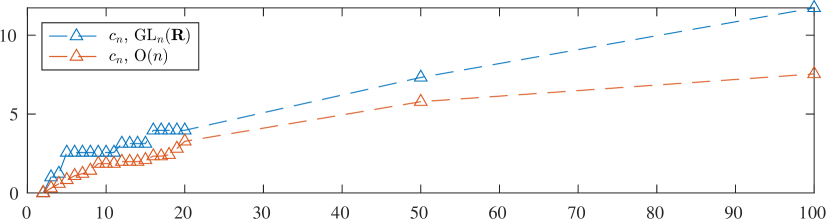
Figure 4: Plot of the computed lower bounds for $c_{n}$.

$n$	2	3	4	5	6	7	8	9	10
$\operatorname{O}(n)$	0	0.2988	0.5852	0.8285	1.0879	1.2194	1.416	1.8546	1.8546
$\operatorname{GL}_{n}(\mathbb{R})$	0	1	1.2277	2.5609	2.5609	2.5609	2.5609	2.5609	2.5609
$n$	11	12	13	14	15	16	17	18	19
$\operatorname{O}(n)$	1.8546	1.9821	1.9821	1.9821	2.0948	2.3315	2.3315	2.4204	2.8118
$\operatorname{GL}_{n}(\mathbb{R})$	2.5609	3.1294	3.1294	3.1294	3.1294	3.9719	3.9719	3.9719	3.9719
$n$	20	50	100
$\operatorname{O}(n)$	3.2711	5.7837	7.5449
$\operatorname{GL}_{n}(\mathbb{R})$	3.9719	7.3208	11.733

Table 3: Computed lower bounds for $c_{n}$ for $\operatorname{O}(n)$ and $\operatorname{GL}_{n}(\mathbb{R})$.

4.2.1 Discussion

This study is intended to provide a starting point for future research into how much larger can GECP growth be than GEPP growth. The particular implementation used here leaves a lot of room for improvement, such as directly using optimization programming (such as JuMP), using parallelization for multiple simultaneous random search steps, as well as using approximate Haar orthogonal sampling methods (such as using butterfly random orthogonal perturbations(see [21, 27])) for more efficient sampling. Future work will explore refinements to this initial study.

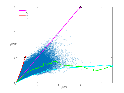
(a) $\operatorname{O}(4)$

(b) $\operatorname{GL}_{4}(\mathbb{R})$

Figure 5: Random search paths using $\varepsilon=10^{-2}$ steps and $M=10^{3}$ neighbor comparisons starting at ${\mathbf{I}}$, using orthogonal $\varepsilon$-steps in (a) and Gaussian $\varepsilon$-steps in (b), with each overlayed on top of plot of $10^{6}$ samples of $\operatorname{Haar}\operatorname{O}(4)$ in (a) and $\operatorname{Ginibre}(4,4)$ in (b). Each included path corresponds to a lower bound random search for $a_{4},b_{4},c_{4},d_{4}$, which are mapped alongside best approximate approximate values for each ensemble.

To better illustrate how a random search path might be constructed, Figure 5 shows sample random search paths starting at the identity matrix, ${\mathbf{I}}$, mapped on top of $10^{6}$ sampled pairs of computed GEPP and GECP growth factors for $\operatorname{Haar}\operatorname{O}(4)$ and $\operatorname{Ginibre}(4,4)$. For comparison, extreme points are included for each set of samples. These include the (scaled) Hadamard point $(4,4)$, which maximizes the GECP growth factor for both maps (i.e., the constant $b_{n}$), the GEPP-GECP growth factor pair $(5.5,\sqrt{11}/2)$ for $Q_{n}$ for $\operatorname{O}(4)$, which provides an approximate maximal GEPP growth and GEPP-GECP growth difference for $\operatorname{O}(4)$ (i.e., $a_{n}$ and $d_{n}$), the points $(8,2)$ for Wilkinson’s worst-case matrix $A_{4}$ and $(8,1)$ for the updated matrix $\tilde{A}_{4}$ (which multiplies the last column of $A_{4}$ by 2) for $\operatorname{GL}_{4}(\mathbb{R})$, which maximize the overall GEPP growth and GEPP-GECP growth difference (i.e, $a_{n}$ and $d_{n}$), along with computed estimated lower bounds for $c_{n}$ for each of $\operatorname{O}(4)$ and $\operatorname{GL}_{4}(\mathbb{R})$ (see Table 3). The best of 5 random search paths for each constant and ensemble were kept.

Remark 4.5.

The identity matrix, ${\mathbf{I}}$, proves a sufficient initial point for a random search to approximate each constant $a_{4},b_{4},c_{4},d_{4}$ for $\operatorname{O}(4)$, as each sampled path ends near the current best estimates for each constant for $\operatorname{O}(4)$ in Figure 5. However, ${\mathbf{I}}$ proves a less successful starting point for $\operatorname{GL}_{4}(\mathbb{R})$. For example, a random search for largest GECP growth factor using Gaussian steps stays essentially bounded by 2 if starting at ${\mathbf{I}}$, as seen in Figure 5(b); this bound essentially holds if starting at $A_{0}\sim\operatorname{Ginibre}(4,4)$. Starting at $A_{0}\sim\operatorname{Haar}\operatorname{O}(4)$ proves more effective at breaking beyond this essential GECP growth boundary for random searches with Gaussian steps: 5 such searches resulted in a best final GECP growth value of 3.901.

Figures 4 and 3 provide some better understanding about how much worse can GECP growth be than GEPP growth. The empirical results support the lower bound estimate

(82) $$c_{n}\geq\mathcal{O}(n^{1/2})$$

for both $\operatorname{O}(n)$ and $\operatorname{GL}_{n}(\mathbb{R})$. More values of $n$ would provide a better lower bound estimate for $c_{n}$. In the least, we would confidently conjecture $c_{n}=\omega(1)$, i.e., GECP can always be progressively worse than GEPP. Note this lower bound estimate appears significantly far from the trivial upper bound for $c_{n}$ of $b_{n}-1\geq\mathcal{O}(n)$, where $b_{n}=g^{\operatorname{GECP}}_{n}$. This contrasts to the result we established for the inverse question of how much worse can GEPP growth be than GECP, which we positively established matched the trivial upper bound of $2^{n-1}-1$ for all matrices.

Also of interest would be to better establish the relationship of $c_{n}$ for both $\operatorname{O}(n)$ and $\operatorname{GL}_{n}(\mathbb{R})$. Comparing the best estimates of $a_{n}$ for both models (i.e, $g^{\operatorname{GEPP}}(\operatorname{O}(n))$ and $g_{n}^{\operatorname{GEPP}}=2^{n-1}$), we established $a_{n}(\operatorname{O}(n))/a_{n}(\operatorname{GL}_{n}(\mathbb{R})=g^{\operatorname{GEPP}}(\operatorname{O}(n))/g_{n}^{\operatorname{GEPP}}=c\cdot(1+o(1))$ for some $c\in[\frac{1}{\sqrt{3}},1)$ in Theorem 3.11. Figures 4 and 3 also support the hypothesis that both constants are of the same order, with each computed ratio satisfying

(83) $$c_{n}(\operatorname{O}(n))/c_{n}(\operatorname{GL}_{n}(\mathbb{R}))\in[0.29,0.83]$$

for each $n$ in our study.

4.3 GEPP and GECP growth factors near extreme points

Using average-case analysis of GEPP in [18], Huang and Tikhomirov establish that polynomial GEPP growth holds with high probability when using small Gaussian perturbations, even when starting with worst-case exponential GEPP growth. We are interested in exploring what can be said explicitly about the polynomial growth that is then encountered on these extreme models.

4.3.1 Larger GECP than GEPP growth

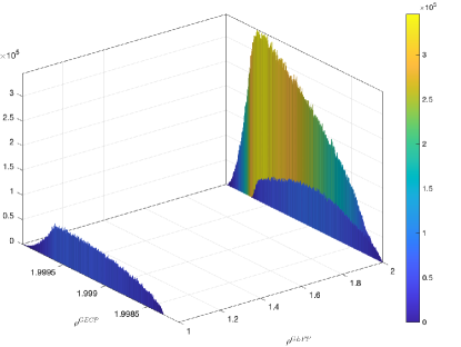
(a) $Q(\boldsymbol{\theta})B_{3}$

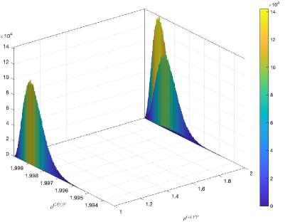
(b) $B_{3}+(\varepsilon/\sqrt{3})G$

Figure 6: Normalized histogram of each pair of $\rho^{\operatorname{GEPP}}$ and $\rho^{\operatorname{GECP}}$ using $10^{6}$ samples of (a) $Q(\boldsymbol{\theta})B_{3}$ for $\boldsymbol{\theta}\sim\operatorname{Uniform}(B_{r}({\mathbf{0}}))\subset\mathbb{R}^{3},r=\varepsilon/\sqrt{6}$, and (b) $B_{3}+(\varepsilon/\sqrt{3})G$ for $G$ for $G\sim\operatorname{Ginibre}(3,3)$, each using $\varepsilon=10^{-3}$.

We will first consider a matrix that has larger GECP growth than GEPP growth. For $n=3$, the matrix $B_{3}$ from (12) satisfies $2=\rho^{\operatorname{GECP}}(B_{3})>\rho^{\operatorname{GEPP}}(B_{3})=1$. We are interested in exploring the behavior for both GEPP and GECP growth on small neighborhoods near $B_{3}$ (although both remain small since $n$ is so small). Figure 6 shows a normalized histogram using a $512\times 512$ grid of computed pairs of GEPP and GECP growth factors in $\varepsilon$-neighborhoods near $B_{3}$ using both orthogonal and additive perturbation methods (see Section 4.1) for $\varepsilon=10^{-3}$.

Stability holds for local GECP growth factors, where all computed GECP growth factors for neighbors of $B_{3}$ stayed within $.005$ of $\rho^{\operatorname{GECP}}(B_{3})=2$. However, the computed GEPP growth factors exhibit highly discontinuous behavior. Each neighbor had GEPP growth that either concentrated only near 1 or 2, and nothing in between. This establishes (empirically) both $(2,1)$ and $(2,2)$ comprise limit points for the mapped pairs of growth factors. Figure 7 shows the plot of each of the GEPP-GECP growth factor pairs for the neighbors that concentrated near the point $(2,2)$, which comprised the right boundary of Figure 6. These nearest neighbors have growth factor pairs that effectively form an arrow that points toward this limit point $(2,2)$.

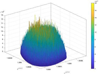
(a) Front view

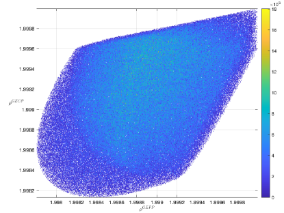
(b) Top view

Figure 7: Local neighborhood near $(\rho^{\operatorname{GEPP}},\rho^{\operatorname{GECP}})=(2,2)$ using orthogonal perturbations $Q(\boldsymbol{\theta})B_{3}$ from Figure 6(a).

What is surprising for this model is that there is higher concentration among these neighbors mapping near $(2,2)$ than the starting point of $(2,1)$. In particular, this shows that while the GECP growth factor remains stable in small neighborhoods, this extreme model has neighbors whose GEPP growth factor moves closer to the larger initial GECP factor. For the $10^{6}$ samples, neighbors were twice as likely to be near $(2,2)$ than $(2,1)$, with 66.68% of the $10^{6}$ samples having computed GEPP growth factors within 0.01 of the initial GECP limit point compared to 33.31% concentrating within 0.01 of the initial GEPP limit point.

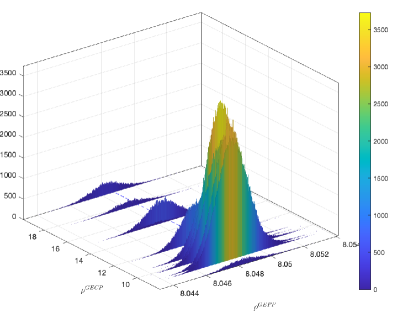
(a) Front view

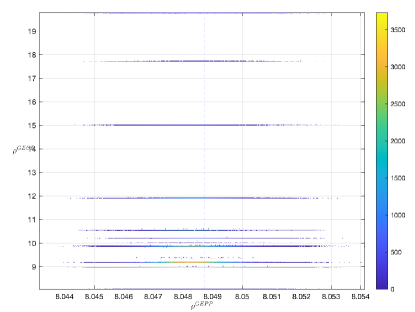
(b) Top view

Figure 8: Normalized histogram of each pair of $\rho^{\operatorname{GEPP}}$ and $\rho^{\operatorname{GECP}}$ using $10^{6}$ samples of $B_{100}+(\varepsilon/10)G$ for $G$ for $G\sim\operatorname{Ginibre}(100,100)$ with $\varepsilon=10^{-3}$, where $B_{100}$ is the computed worst-case matrix that maximizes the GECP-GEPP growth for $n=100$, with initial $(\rho^{\operatorname{GEPP}},\rho^{\operatorname{GECP}})=(8.0487,19.7819)$. A plot of the line $\rho^{\operatorname{GEPP}}=8.0487$ is included for comparison.

This behavior does not hold for the remaining computed matrices used for the best lower bounds for $c_{n}$ from Table 3. For $n\geq 4$, each of the other computed maximal GECP-GEPP difference models maintained stable GEPP growth factors, with all $10^{6}$ samples for each $n$ having computed GEPP growth factors stay within 0.02 of the starting GEPP growth factor; so only one limit point held for the GEPP growth factors. However, for these models then the larger initial GECP growth factor showed less stability: as $n$ increased, then the computed GECP growth factors for neighbors moved progressively away from the larger initial GECP growth factor and closer to the smaller initial GEPP growth factor. Figure 8 shows a plot of the computed GEPP and GECP growth factors for $\varepsilon$-neighbors of $B_{100}$, which has the computed maximal GECP-GEPP growth difference for $100\times 100$ matrices of $11.7332$, with $\rho^{\operatorname{GEPP}}(B_{100})=8.0487$ and $\rho^{\operatorname{GECP}}(B_{100})=19.7819$. This model exhibits stable GEPP growth factors but highly discontinuous GECP growth factors that are much more concentrated near 8.0487 than 19.7819. $B_{100}$ also exhibits the first positive proportion (0.07%) of the $10^{6}$ sampled neighboring GECP growth factors appearing within 0.01 of the initial GEPP growth factor among all cases $n=2:20,50$.

4.3.2 Larger GEPP than GECP growth

We will next consider the local behavior of the GEPP and GECP growth factors when the initial GEPP growth factor is much larger than the GECP growth factor. First, we will consider neighborhoods of $Q_{4}$, which maps to the point

(84) $$(\rho^{\operatorname{GEPP}}(Q_{4}),\rho^{\operatorname{GECP}}(Q_{4}))=(11/2,\sqrt{11},2)\approx(5.5,1.658312395).$$

$Q_{n}$ exhibits exponential GEPP growth of order $(2^{n-1}/\sqrt{3})(1+o(1))$ by Corollary 3.3 and a small GECP growth factor that (empirically) concentrates on $\sqrt{2}$. Figure 9 exhibits the local GEPP and GECP growth behavior near $Q_{4}$, which shows a normalized histogram on a $512\times 512$ grid for $10^{6}$ sampled $\varepsilon$-neighbors from both multiplicative and additive perturbations methods with $\varepsilon=10^{-3}$ (see Section 4.1).

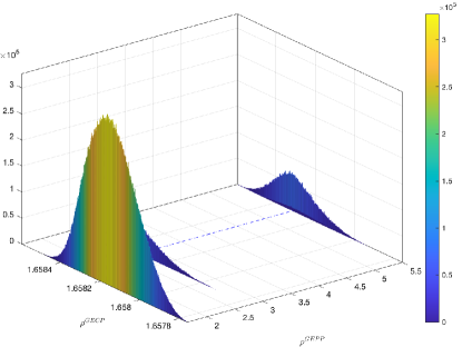
(a) $Q(\boldsymbol{\theta})Q_{4}$

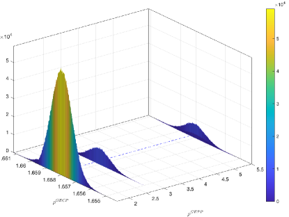
(b) $Q_{4}+(\varepsilon/2)G$

Figure 9: Normalized histogram of each pair of $\rho^{\operatorname{GEPP}}$ and $\rho^{\operatorname{GECP}}$ using $10^{6}$ samples of (a) $UQ_{4}$ for $U=Q(\boldsymbol{\theta})$, $\boldsymbol{\theta}\sim\operatorname{Uniform}(B_{r}({\mathbf{0}}))\subset\mathbb{R}^{6},r=\varepsilon/\sqrt{12}$, and (b) $Q_{4}+(\varepsilon/2)G$ for $G$ for $G\sim\operatorname{Ginibre}(4,4)$, each using $\varepsilon=10^{-3}$. The line $\rho^{\operatorname{GECP}}=\sqrt{11}/2$ is included for comparison.

	$X_{n}=\rho^{\operatorname{GECP}}(Q_{n})-\rho^{\operatorname{GEPP}}(Q_{n}+\overline{G})$				$Y_{n}=\rho^{\operatorname{GECP}}(A_{n})-\rho^{\operatorname{GEPP}}(A_{n}+\overline{G})$
$n$	Median	$\overline{x}$	$s$	$\approx\mathbb{P}(X_{n}=0)$	Median	$\overline{x}$	$s$	$\approx\mathbb{P}(Y_{n}=0)$
2	2.84e-3	0.0032	0.0019	0.9961	2.01e-3	0.0023	0.0013	1.0000
3	-9.31e-5	-0.4199	0.5958	0.6669	9.89e-4	-0.6637	0.9404	0.6665
4	1.00e-5	-0.6419	1.3045	0.7498	9.84e-4	-0.9030	1.8486	0.7505
5	5.52e-5	-0.9290	2.4497	0.7995	9.17e-4	-0.9396	2.6996	0.8001
6	7.63e-5	-1.4046	4.4950	0.8330	8.49e-4	-0.9144	3.6066	0.8333
7	9.50e-5	-2.2121	8.1828	0.8573	7.89e-4	-0.8642	4.6407	0.8573
8	1.25e-4	-3.5869	14.747	0.8748	7.37e-4	-0.8128	5.9164	0.8755
9	1.12e-4	-5.8481	26.175	0.8887	6.92e-4	-0.7732	7.6716	0.8889
10	1.13e-4	-9.6106	45.923	0.9001	6.53e-4	-0.7222	9.5064	0.8999
11	1.14e-4	-15.614	78.089	0.9091	6.19e-4	-0.6990	12.557	0.9092
12	1.14e-4	-23.934	124.76	0.9165	5.90e-4	-0.6236	14.360	0.9169
13	1.12e-4	-34.364	185.42	0.9231	5.65e-4	-0.5931	16.586	0.9230
14	1.88e-4	-46.564	255.24	0.9281	5.41e-4	-0.5514	19.812	0.9284
15	1.29e-4	-57.685	322.47	0.9333	5.22e-4	-0.4736	18.366	0.9336
16	1.08e-4	-67.262	382.40	0.9379	5.03e-4	-0.4586	23.037	0.9375
17	1.08e-4	-76.783	440.15	0.9411	4.87e-4	-0.4781	24.960	0.9413
18	1.05e-4	-84.588	486.28	0.9442	4.72e-4	-0.4483	25.173	0.9442
19	1.05e-4	-89.732	521.30	0.9475	4.59e-4	-0.3602	15.770	0.9473
20	1.04e-4	-94.261	549.62	0.9502	4.46e-4	-0.3140	13.059	0.9507
50	1.82e-4	-99.268	783.61	0.9800	2.82e-4	-0.1059	8.9006	0.9798
100	1.62e-4	-74.840	817.42	0.9900	2.06e-4	-0.0599	13.495	0.9900

Table 4: Summary statistics (median, mean, standard deviation) for $10^{6}$ samples of $\varepsilon$-neighbors for the difference of initial GECP growth factor to neighbor GEPP growth factor for each of $Q_{n}$ and $A_{n}$, with $\varepsilon=10^{-3}$, $n=2:20,50,100$, using $\mathbb{P}(|X_{n}|<\operatorname{tol})\approx\mathbb{P}(X_{n}=0)$ for $\operatorname{tol}=0.01$ and similarly $\mathbb{P}(|Y_{n}|<\operatorname{tol})\approx\mathbb{P}(Y_{n}=0)$.

The small initial GECP growth factor results in highly stable GECP growth behavior, with all $10^{6}$ samples remaining within $0.002$ of $\rho^{\operatorname{GECP}}(Q_{4})=\sqrt{11}/2\approx 1.6583$. Conversely, the local GEPP growth behavior is now highly discontinuous, with all computed $\varepsilon$-neighbor GEPP growth factors staying within $0.002$ of either $\rho^{\operatorname{GEPP}}(Q_{4})=5.5$, $5.5/2$, or the smaller initial GECP growth factor of $1.6583$. Of these three values, most $\varepsilon$-neighbors concentrate near the smallest limit point, with 2/3 of the additive $\varepsilon$-neighbors having computed GEPP growth within $0.01$ of $1.6583$. This concentration near $\rho^{\operatorname{GECP}}(Q_{n})=\sqrt{2}\cdot(1+o(1))$ increases with $n$, where $10^{6}$ samples for different $n$ yield the approximation

(85) $$\mathbb{P}\left(\rho^{\operatorname{GEPP}}(Q_{n}+(\varepsilon/\sqrt{n})G)=\rho^{\operatorname{GECP}}(Q_{n})\right)\approx 1-\frac{1}{n}.$$

Similar behavior was also observed for Wilkinson’s worst-case GEPP matrices, $A_{n}$, with again approximately $1-\frac{1}{n}$ of sampled GEPP growth factors concentrating near $\rho^{\operatorname{GECP}}(A_{n})=2$ (see Table 4 for summary statistics for $\varepsilon$-neighbors of both $Q_{n}$ and $A_{n}$). Hence, for both exponential GEPP growth models $Q_{n}$ and $A_{n}$, the local GEPP growth factors using Gaussian perturbations limit to the initial GECP growth factor for each model.

4.3.3 Discussion

For each of the extreme models studied, one of the GEPP or GECP growth factors remained stable while the other exhibited highly discontinuous behavior in both orthogonal multiplicative and Gaussian additive neighborhoods. With the exception of $B_{3}$, which had local GEPP growth concentrate closer to the larger initial GECP growth, every other extreme studied in this section exhibited stable growth for the pivoting strategy with smaller initial growth factor while the other growth has local behavior that progressively concentrates near the smaller initial growth factor. This limiting behavior is further exhibited by each computed pair of $(\rho^{\operatorname{GEPP}},\rho^{\operatorname{GECP}})$ for $\varepsilon$-neighbors staying near the line connecting $(\rho^{\operatorname{GEPP}}(A_{0}),\rho^{\operatorname{GECP}}(A_{0}))$ and $(m,m)$ for $m=\min\{\rho^{\operatorname{GEPP}}(A_{0}),\rho^{\operatorname{GECP}}(A_{0})\}$.

This gives further qualification of the result of Huang and Tikhomirov in [18], who found that using GEPP with small Gaussian perturbations leads to growth factors that are at most polynomially large with high probability despite exponential worst-case growth. Empirically, what we are actually seeing on particular exponential GEPP growth models is using GEPP with small perturbations leads to GECP behavior, which then appears polynomial: so higher stability using GEPP and random perturbations follows from higher stability properties of GECP.

Appendix A Background and notation

We will restrict focus to $n\times n$ matrices with real entries, $\mathbb{R}^{n\times n}$. Let $A_{ij}$ denote the element in row $i$ and column $j$ for a matrix $A\in\mathbb{R}^{n\times n}$. For indices $\alpha,\beta\subset[n]:=\{1,2,\ldots,n\}$, let $A_{\alpha,\beta}$ denote the submatrix of $A$ built using the entries $A_{ij}$ for $i\in\alpha,j\in\beta$. Standard notation (as in MATLAB) will be used for consecutive sequences $j:k=j,j+1,\ldots,k-1,k$, while a colon “$:$” is used if $\alpha=[n]$ or $\beta=[n]$ (e.g., $A_{:,j}=A{\mathbf{e}}_{j}$ denotes the $j^{th}$ column of $A$). For $A\in\mathbb{R}^{n\times n}$, let $|A|$ denote the matrix with entries $|A|_{ij}=|A_{ij}|$, i.e., apply the absolute value entrywise to $A$. Let $\|A\|_{\max}=\max_{i,j}|A_{ij}|$ denote the max-norm and $\|A\|_{p}$ the induced matrix norm from the vector norms $\|{\mathbf{x}}\|_{p}=(x_{1}^{p}+\cdots x_{n}^{p})^{1/p}$ for ${\mathbf{x}}\in\mathbb{R}^{n}$. Let ${\mathbf{e}}_{i}$ denote the standard basis element of $\mathbb{R}^{n}$ whose $i^{th}$ component is 1 and 0 elsewhere, and ${\mathbf{E}}_{ij}={\mathbf{e}}_{i}{\mathbf{e}}_{j}^{T}$ denote the basis elements of $\mathbb{R}^{n\times n}$. Let ${\mathbf{I}}=\sum_{i}{\mathbf{E}}_{ii}$ denote the identity matrix and ${\mathbf{0}}$ the zero matrix, whose dimensions are explicitly stated if not implicitly obvious.

Let $\operatorname{GL}_{n}(\mathbb{R})\subset\mathbb{R}^{n\times n}$ denote the group of nonsingular matrices and $\operatorname{O}(n)=\{Q\in\operatorname{GL}_{n}(\mathbb{R}):QQ^{T}={\mathbf{I}}\}$ the subgroup of orthogonal matrices. Note this notation differs in this document from $\mathcal{O}(n)$, which denotes the standard big-O notation, with $f(n)=\mathcal{O}(g(n))$ when there exists a constant $c>0$ such that for all sufficiently large $n$, $|f(n)|\leq c|g(n)|$. Other standard complexity notation that will be used includes small-o notation (i.e., $f(n)=o(g(n))$ when$\displaystyle\lim_{n\to\infty}f(n)/g(n)=0$), $f(n)=\omega(g(n))$ when $\displaystyle\lim_{n\to\infty}|f(n)/g(n)|=\infty$, and big-$\Theta$ notation $f(n)=\Theta(g(n))$ when $f(n)=\mathcal{O}(g(n))$ and $g(n)=\mathcal{O}(f(n))$. Let $\epsilon=\epsilon_{\operatorname{machine}}$ denote the machine epsilon, which is the smallest positive number such that $\operatorname{fl}(1+\epsilon)\neq 1$ when using floating-point arithmetic. If using $t$-bit mantissa, then $\epsilon=2^{-t}$. Later experiments will use double precision in MATLAB, which has 52-bit mantissa.

Standard numerical linear algebra textbooks (e.g., [15, 26]) give a thorough overview of standard implementations of GE and QR factorizations. In short, GE applied to a matrix $A\in\operatorname{GL}_{n}(\mathbb{R})$ iteratively builds up each factor to provide a final matrix factorization $PAQ=LU$, where $L$ is a unipotent lower triangular matrix, $U$ is upper triangular, and $P,Q$ are permutation matrices that account for the row and columns swaps needed by the chosen pivoting strategy. $A^{(k)}$ will denote the intermediate GE form of $A$ before the $k^{th}$ GE step with 0’s below the first $(k-1)$st diagonal entries, where $A^{(1)}=A$ and $A^{(n)}=U$. For $L^{(k)}$ be the associated intermediate form of $L$, then $A^{(k)}=[L^{(k)}]^{-1}A$. GE with no pivoting (GENP) uses $P=Q={\mathbf{I}}$, but is only possible if no principal minors of $A$ vanish, i.e., when $A$ is block nondegenerate. GE with partial pivoting (GEPP) uses only row swaps to ensure the leading column of the untriangularized part of $A^{(k)}$ has maximal magnitude at the leading pivot entry (i.e., $Q={\mathbf{I}}$); this results also in each row cancellation factor $L_{ij}=-A^{(j)}_{ij}/A^{(j)}_{jj}$ satisfying $|L_{ij}|\leq 1$ for all $i>j$ so that $\|L\|_{\max}=1$. GE with complete pivoting (GECP) uses row and column swaps to ensure the leading pivot is maximal in magnitude in the entire remaining untriangularized lower $(n-k+1)\times(n-k+1)$ block.

Recall every matrix $A\in\operatorname{GL}_{n}(\mathbb{R})$ has a QR factorization $A=QR$ for $Q\in\operatorname{O}(n)$ and $R$ upper triangular with positive diagonal. QR and GENP factorizations on nonsingular matrices then are unique. Recall a QR factorization can be attained through the use of Householder reflectors or Givens rotations, $G(\theta,i,j)$, which is the identity matrix updated so that $G(\theta,i,j)_{[i\ j],[i\ j]}=\begin{bmatrix}\cos\theta&\sin\theta\\ -\sin\theta&\cos\theta\end{bmatrix}$. Our experiments in later sections will use Householder reflectors to efficiently sample Haar orthogonal matrices (see below), as outlined in more detail in [20], along with Givens rotations with sufficiently small input angles to keep a product inside an $\varepsilon$ neighborhood of a matrix (see [13] for a similar approach).

A matrix $A\in\operatorname{GL}_{n}(\mathbb{R})$ is called partially pivoted (PP) if no row pivots are ever needed during its GEPP factorization so that its GENP and GEPP factorizations align. Equivalently, $A$ is PP if its GENP factorization $A=LU$ satisfies $\|L\|_{\max}=1$. $A$ is completely pivoted (CP) if no pivots are ever needed during its GECP factorization. A check for CP is more involved than that for PP. For example, $A$ is CP iff for each $k=1:n$ the magnitude of the determinant of the inverse of the lower principal $n-k+1$ submatrix of $A^{(k)}$ is maximized among all possible row or column permutations [6].

For random variables $X,Y$, let $X\sim Y$ denote that $X$ and $Y$ are equal in distribution. Standard distributions that will be referenced include the standard (real) Gaussian $X\sim N(\mu,\sigma^{2})$, with density $(2\pi\sigma^{2})^{-1/2}\exp((x-\mu)^{2}/(2\sigma^{2}))$, and uniform random variables $X\sim\operatorname{Uniform}(\mathcal{S})$ with density $(1/|\mathcal{S}|)\mathds{1}(x\in\mathcal{S})$, where $|\mathcal{S}|$ denotes the cardinality of $\mathcal{S}$ if $\mathcal{S}$ is finite and the standard Lebesgue measure of $\mathcal{S}$ is $\mathcal{S}$ is pre-compact. For $G$ a compact Hausdorff topological group, then there exists a left and right invariant regular probability Haar measure on $G$, $\operatorname{Haar}(G)$ [29]. Certain Haar and uniform measures can be sampled using standard Gaussian ensembles called the Ginibre ensembles, $\operatorname{Ginibre}(n,m)=\{A\in\mathbb{R}^{n\times m}:A_{ij}\mbox{ iid }N(0,1)\}$. For example, for $\mathbb{S}^{n-1}=\{{\mathbf{x}}\in\mathbb{R}^{n}:\|{\mathbf{x}}\|_{2}=1\}$, if ${\mathbf{x}}\sim\operatorname{Ginibre}(n,1)$, then ${\mathbf{x}}/\|{\mathbf{x}}\|_{2}\sim\operatorname{Uniform}(\mathbb{S}^{n-1})$; for $B_{\varepsilon}({\mathbf{0}})=\{{\mathbf{x}}\in\mathbb{R}^{n}:\|{\mathbf{x}}\|_{2}\leq\varepsilon\}$, if ${\mathbf{x}}\sim\operatorname{Ginibre}(n+2,1)$, then $(\varepsilon/\|{\mathbf{x}}\|_{2})[{\mathbf{I}}_{n}\ {\mathbf{0}}]{\mathbf{x}}\sim\operatorname{Uniform}(B_{\varepsilon}({\mathbf{0}}))$; if $A\sim\operatorname{Ginibre}(n,n)$ has QR factorization $A=QR$ (where $R$ has positive diagonal), then $Q\sim\operatorname{Haar}\operatorname{O}(n)$. The last example, first established by Stewart in [24], uses the orthogonal invariance of $\operatorname{Ginibre}(n,m)$, i.e., if $A\sim\operatorname{Ginibre}(n,m)$ and $U\in\operatorname{O}(n),V\in\operatorname{O}(m)$ then $UAV^{*}\sim A$.

Appendix B Proofs of results in Section 3

First we will prove Proposition 3.1, which establishes the explicit intermediate GEPP forms $Q_{n}^{(k)}$ for $Q_{n}$, the orthogonal QR factor for $L_{n}$.

Proof B.1 (Proof of Proposition 3.1).

To show $Q_{n}$ is orthogonal, one needs to show $\hat{Q}^{T}\hat{Q}=\hat{D}$, and to see the orthogonal QR factor aligns with $Q_{n}$, one needs to show $\hat{Q}^{T}L_{n}$ or equivalently $L_{n}^{-1}\hat{Q}$ is upper triangular with positive diagonal. This last step will also then establish each intermediate $\hat{Q}^{(k)}$ form as well.

A check $\hat{Q}_{:,j}^{T}\hat{Q}_{:,j}=\hat{D}_{jj}$ follows directly from (29), (32), (36) along with the identity

(86) $$\alpha_{n}+1=4\alpha_{n-1}.$$

By construction $\hat{Q}_{:,n-1}^{T}\hat{Q}_{:,j}=0$ for all $j\neq n-1$ is clear since $Q_{n-1:n,j}$ is a scalar multiple of $\begin{bmatrix}1\\ 1\end{bmatrix}$ for all $j\neq n-1$ while $Q_{:,n-1}={\mathbf{e}}_{n-1}-{\mathbf{e}}_{n}$. Now note for $n>2$ and $j<n-1$, (32) and (36) can be rewritten as

(87) $$\hat{Q}_{:,n} ={\mathbf{e}}_{n}+\sum_{k=1}^{n-1}2^{n-1-k}{\mathbf{e}}_{k}$$

(88) $$\hat{Q}_{:,j} =-(n-j-1)\sum_{i=1}^{j-1}2^{j-i-1}{\mathbf{e}}_{i}+[(n-j)(\alpha_{j}-1)+1]{\mathbf{e}}_{j}-\alpha_{j}\sum_{i=j+1}^{n}{\mathbf{e}}_{i}.$$

It follows

$$\hat{Q}_{:,n}^{T}\hat{Q}_{:,j} ={\mathbf{e}}_{n}^{T}\hat{Q}_{:,j}+\sum_{k=1}^{j-1}2^{n-1-k}{\mathbf{e}}_{k}^{T}\hat{Q}_{:,j}+2^{n-1-j}{\mathbf{e}}_{j}^{T}\hat{Q}_{:,j}+\sum_{k=j+1}^{n-1}2^{n-1-k}{\mathbf{e}}_{k}^{T}\hat{Q}_{:,j}$$

$$=-\alpha_{j}-(n-j-1)\sum_{k=1}^{j-1}2^{n+j-2-2k}+2^{n-1-j}[(n-j)(\alpha_{j}-1)+1]-\alpha_{j}\sum_{k=j+1}^{n-1}2^{n-1-k}$$

$$=-\alpha_{j}-(n-j-1)2^{n-1-j}(\alpha_{j}-1)+2^{n-1-j}[(n-j)(\alpha_{j}-1)+1]-\alpha_{j}(2^{n-1-j}-1)$$

$$=0$$

Next, note

(89) $$\hat{Q}_{:,1}={\mathbf{e}}_{1}-\sum_{j=2}^{n}{\mathbf{e}}_{j}$$

so that for $n\geq 4$ and $2\leq j\leq n-2$, then

$$\hat{Q}_{:,1}^{T}\hat{Q}_{:,j} =(n-j-1)\left[-2^{j-2}+\sum_{i=2}^{j-1}2^{j-i-1}\right]-[(n-j)(\alpha_{j}-1)+1]+\alpha_{j}\sum_{i=j+1}^{n}1$$

$$=-(n-j-1)-(n-j)(\alpha_{j}-1)-1+(n-j)\alpha_{j}$$

$$=0$$

When $n\geq 5$, an analogous and straightforward computation yields for $2\leq i<j\leq n-2$

$$\hat{Q}^{T}_{:,i}\hat{Q}_{:,j} =(n-i-1)(n-j-1)2^{j-i-1}(\alpha_{i}-1)-[(n-i)(\alpha_{i}-1)+1](n-j-1)2^{j-i-1}$$

$$\qquad+\alpha_{i}(n-j-1)(2^{j-i-1}-1)-\alpha_{i}[(n-j)(\alpha_{j}-1)+1]+\alpha_{i}\alpha_{j}(n-j)$$

$$=0.$$

This establishes $\hat{Q}^{T}\hat{Q}=\hat{D}$.

Recall for $L_{n}^{(k)}$ the form of $L_{n}$ at GE step $k$, then we can write $[L^{(k)}]^{-1}\hat{Q}=\hat{Q}^{(k)}$. Recall also $L_{n}^{-1}$ acts on a matrix on the left by iteratively adding each row to every row below it. This last property can be reformulated as

(92) $${\mathbf{e}}_{i}^{T}[L_{n}^{(k)}]^{-1}{\mathbf{x}} =\left\{\begin{array}[]{cl}\displaystyle x_{i}+\sum_{\ell=1}^{k-1}2^{k-1-\ell}x_{\ell},&i>k\\ \displaystyle x_{i}+\sum_{\ell=1}^{i-1}2^{i-1-\ell}x_{\ell},&i\leq k\\ \end{array}\right.$$

for any ${\mathbf{x}}\in\mathbb{R}^{n}$. Using (32) and the fact

(93) $$\sum_{\ell=1}^{m-1}2^{k-1-\ell}2^{n-\ell-1}=2^{n+k-2m-1}(\alpha_{m}-1),$$

yields then directly (49), using also (86) for the $k=i=n$ case along with $1+\frac{1}{2}(\alpha_{n}-1)=2\alpha_{n-1}$. (43) follows even more directly from (29).

Since

(94) $$\hat{Q}_{1:j-1,j}=-(n-j-1)\begin{bmatrix}2^{j-i-1}\\ \vdots\\ 2\\ 1\end{bmatrix}=-(n-j-1)\hat{Q}_{n-j+1:n-1,n}$$

we can reuse (49), the intermediate forms for the last column of $Q$, to then yield (58); note also $\hat{Q}_{ij}^{(k)}=0$ for $k>j$ and $i>j$ since for $k=j$, then

(95) $$\hat{Q}_{jj}^{(j)} =[(n-j)(\alpha_{j}-1)+1]-(n-j-1)2^{-1}(\alpha_{j}-1)$$

(96) $$=\frac{1}{2}(n-j+1)(\alpha_{j}-1)+\frac{1}{2}(\alpha_{j}+1)$$

(97) $$\hat{Q}_{ij}^{(j)} =-\left[\alpha_{j}+(n-j-1)2^{-1}(\alpha_{j}-1)\right]=-\hat{Q}_{jj}^{(j)}$$

so the following $(j+1)$-GE step necessarily eliminates all entries below the $jj$ entry. Since then $0=\hat{Q}_{ij}^{(j+1)}=\hat{Q}_{ij}^{(j+2)}=\cdots=\hat{Q}_{ij}^{(n)}$, this establishes $L_{n}^{-1}\hat{Q}=\hat{Q}^{(n)}$ is upper triangular. Moreover, since

(98) $$\hat{Q}_{jj}^{(n)} =1+\frac{1}{2}(n-j+1)(\alpha_{j}-1),\qquad j<n-1$$

(99) $$\hat{Q}_{n-1,n-1}^{(n)} =1,$$

(100) $$\hat{Q}_{nn}^{(n)} =2\alpha_{n-1},$$

then $\hat{Q}^{(n)}$ has positive diagonal.

Next, we will use Proposition 3.1 to establish the asymptotic GEPP growth factor for $Q_{n}$.

Proof B.2 (Proof of Corollary 3.3).

Using (58) for $2\leq j\leq n-2$, we have each GENP (and GEPP) intermediate form $\hat{Q}^{(k)}$ satisfies

(101) $$\max_{k}\|\hat{Q}_{1:j-1,j}^{(k)}\|_{\infty} =|\hat{Q}_{j-1,j}^{(n)}|=(n-j-1)\alpha_{j-1}$$

(102) $$\max_{k}\|\hat{Q}_{jj}^{(k)}\|_{\infty} =|\hat{Q}_{jj}|=(n-j)(\alpha_{j}-1)+1$$

(103) $$\max_{k}\|\hat{Q}_{j+1:n,j}^{(k)}\|_{\infty} =|\hat{Q}^{(j)}_{j+1,j}|=\frac{1}{2}(n-j+1)(\alpha_{j}-1)+2\alpha_{j-1}.$$

Since also

(104) $$\max_{k}\|\hat{Q}^{(k)}_{:,1}\|_{\infty} =|\hat{Q}_{11}|=1=|\hat{Q}_{n-1,n-1}|=\max_{k}\|\hat{Q}^{(k)}_{:,n-1}\|_{\infty}$$

then

(105) $$\max_{k}\|\hat{Q}^{(k)}_{:,j}\|_{\max}=|\hat{Q}_{jj}|\quad\mbox{for all $j\leq n-1$.}$$

Together, this shows

(106) $$\max_{k}\|Q^{(k)}_{:,1:n-1}\|_{\max}=\max_{k}\{|\hat{Q}_{jj}|D_{jj}^{-1/2}:\ j=1,\ldots,n-1\}\leq\|Q\|_{\max}\leq\|Q\|_{2}=1,$$

while by (49) we have

(107) $$\max_{k}\|Q^{(k)}_{:,n}\|_{\infty}=|\hat{Q}^{(n)}_{nn}|D^{-1/2}_{nn}=2\alpha_{n-1}D_{nn}^{-1/2}=\sqrt{2\alpha_{n-1}}>1.$$

This yields

(108) $$\max_{k}\|Q^{(k)}\|_{\max}=\sqrt{2\alpha_{n-1}}.$$

Moreover, by Proposition 3.1, we have

$$|Q_{jj}| =|\hat{Q}_{jj}|D_{jj}^{-1/2}$$

$$=\frac{(n-j)(\alpha_{j}-1)+1}{\left[(n-j)^{2}(\alpha_{j}-1)^{2}\cdot\frac{2\alpha_{j}-1}{2\alpha_{j}-2}+(n-j)(\alpha_{j}^{2}+\alpha_{j}-1)+2\alpha_{j-1}\right]^{1/2}}$$

$$=\sqrt{\frac{2\alpha_{j}-2}{2\alpha_{j}-1}}\frac{1+\Theta\left(\frac{1}{(n-j)\alpha_{j}}\right)}{\left[1+\Theta(\frac{1}{n-j})+\Theta(\frac{1}{(n-j)\alpha_{j}})\right]^{1/2}}$$

for each $j\leq n-2$. Taking $j=j(n)$ so that $n-j=\omega_{n}(1)$ , then

(109) $$1+o(1)=|Q_{j(n),j(n)}|\leq\|Q\|_{\max}\leq 1\qquad\mbox{and so also }\qquad\|Q\|_{\max}^{-1}=1+o(1).$$

Note

(110) $$\sqrt{2\alpha_{n-1}}=\left[2\left(1+\frac{2}{3}(4^{n-2}-1)\right)\right]^{1/2}=\frac{2^{n-1}}{\sqrt{3}}\sqrt{1+2^{3-2n}}=\frac{2^{n-1}}{\sqrt{3}}(1+o(1)).$$

Combining (109) and (110) along with the fact $\|L\|_{\max}=1$ yields

(111) $$\rho^{\operatorname{GEPP}}(Q)=\frac{\displaystyle\|L\|_{\max}\max_{k}\|Q^{(k)}\|_{\max}}{\|Q\|_{\max}}=\frac{2^{n-1}}{\sqrt{3}}(1+o(1)).$$

Last, we will show the maximal growth encountered for orthogonal matrices at any intermediate GEPP step is attained by any orthogonal matrix of the form $Q=DQ_{n}\tilde{D}$ for sign diagonal matrices $D,\tilde{D}$.

Proof B.3 (Proof of Proposition 3.12).

Let $Q\in\operatorname{O}(n)$. For $L_{ij}=Q^{(j)}_{ij}/Q^{(j)}_{jj}$, then

(112) $$Q^{(k)}_{ij} =Q_{ij}+\sum_{\ell=1}^{\min(i,k)-1}\left(\sum_{\mathcal{J}\in\mathcal{T}(\min(i,k),\ell)}\prod_{e(r,s)\in\mathcal{J}}(-L_{rs})\right)Q_{\ell j},$$

where

(113) $$\mathcal{T}(n,m)=\{\{e(i_{0},i_{1}),e(i_{1},i_{2}),\ldots,e(i_{k-1},i_{k})\}:n=i_{0}>i_{1}>\cdots>i_{k}=m\}$$

is the collection of decreasing paths in $\mathcal{K}_{n}$, the complete graph on $n$ vertices, connecting vertices $n>m$. Note $|\mathcal{T}(n,1)|=2|\mathcal{T}(n-1,1)|$ since half of the decreasing paths connecting vertices $n$ to 1 skip vertex $n-1$. Since $|\mathcal{T}(n,m)|=|\mathcal{T}(n-m+1,1)|$ and $|\mathcal{T}(2,1)|=1$, then

(114) $$|\mathcal{T}(n,m)|=2^{n-m-1}.$$

Using the triangle inequality along with the fact $|L_{ij}|\leq 1$ for all $i,j$, we have

(115) $$|Q^{(k)}_{ij}|\leq|Q_{ij}|+\sum_{\ell=1}^{\min(i,k)-1}2^{\min(i,k)-\ell-1}|Q_{\ell j}|=f_{\min(i,k),i}(|Q{\mathbf{e}}_{j}|)$$

where

(116) $$f_{r,s}({\mathbf{x}}) =f_{r}([x_{1},\ldots,x_{r-1},x_{s}]^{T})\qquad\mbox{for}\qquad r\leq s,\qquad\mbox{using}$$

(117) $$f_{r}({\mathbf{y}}) =y_{r}+\sum_{\ell=1}^{r-1}2^{r-\ell-1}y_{\ell}$$

for ${\mathbf{x}}\in\mathbb{R}^{n}$ and ${\mathbf{y}}\in\mathbb{R}^{r}$. Next, note for $r<s$ and ${\mathbf{x}}=|{\mathbf{x}}|$, then

(118) $$f_{n}({\mathbf{x}})\geq f_{s,s}({\mathbf{x}})=x_{s}+\sum_{\ell=r+1}^{s-1}2^{s-\ell-1}x_{\ell}+2^{s-r-1}\left(x_{r}+2\sum_{\ell=1}^{r-1}2^{r-\ell-1}x_{\ell}\right)>f_{r,s}({\mathbf{x}}).$$

It follows

(121) $$\max_{\footnotesize\begin{array}[]{c}1\leq i,k\leq n\\ {\mathbf{x}}\in\mathbb{S}^{n-1}\end{array}}{f_{\min(i,k),i}({\mathbf{x}})}=\max_{{\mathbf{x}}\in\mathbb{S}^{n-1}}{f_{n}({\mathbf{x}})}.$$

Maximizing the objective function $f_{n}({\mathbf{x}})$ given the constraint ${\mathbf{x}}\in\mathbb{S}^{n-1}$ (say, using a Lagrange multiplier method with $g({\mathbf{x}})=\|{\mathbf{x}}\|_{2}^{2}=1$) yields the maximum $f(\hat{{\mathbf{x}}})=\sqrt{2\alpha_{n-1}}$ with unique maximizer $\hat{{\mathbf{x}}}={\mathbf{y}}/\sqrt{2\alpha_{n-1}}\in\mathbb{R}^{n}$ with $y_{j}=2^{n-1-j}$ for $j<n$ and $y_{n}=1$. This is precisely the last column of the orthogonal matrix $Q_{n}$ from Proposition 3.1.

By Corollary 3.8, if $Q\in\mathcal{Q}_{n}$, then

(122) $$\|Q^{(k)}\|_{\max}\leq\|Q^{(n)}\|_{\max}=f_{n}(\hat{{\mathbf{x}}})=\sqrt{2\alpha_{n-1}}.$$

Conversely, suppose $\tilde{Q}\in\operatorname{O}(n)$ attains this maximum. Let $m,i,j$ be such that $|\tilde{Q}^{(m)}_{ij}|=\displaystyle\max_{k}\|\tilde{Q}^{(k)}\|_{\max}$. Let $D$ be a sign matrix such that $D\tilde{Q}{\mathbf{e}}_{j}=|Q{\mathbf{e}}_{j}|$, and let ${\mathbf{x}}=D\tilde{Q}{\mathbf{e}}_{j}$ (so that $\|{\mathbf{x}}\|_{2}=1)$. Then

(123) $$f_{n}(\hat{{\mathbf{x}}})=|\tilde{Q}^{(m)}_{ij}|\leq f_{\min(m,i),i}({\mathbf{x}})\leq f_{n}(\hat{{\mathbf{x}}}).$$

It follows $i=j=m=n$ and ${\mathbf{x}}=\hat{{\mathbf{x}}}$ by (118) and (121) and the uniqueness of the maximizer in the above computation. Let $\tilde{D}$ be such that $Q=D\tilde{Q}\tilde{D}$ has positive diagonal and last column, where now ${\mathbf{x}}=Q{\mathbf{e}}_{n}$. So

(124) $$|\tilde{Q}^{(n)}_{nn}| =Q^{(n)}_{nn}=x_{n}+\sum_{\ell=1}^{n-1}\left(\sum_{\mathcal{J}\in\mathcal{T}(n,\ell)}\prod_{e(r,s)\in\mathcal{J}}(-L_{rs})\right)x_{\ell}=f_{n}(\hat{{\mathbf{x}}})$$

so that

(125) $$2^{n-1-\ell} =|\mathcal{T}(n,\ell)|=\left|\sum_{\mathcal{J}\in\mathcal{T}(n,\ell)}\prod_{e(r,s)\in\mathcal{J}}(-L_{rs})\right|\quad\mbox{for all $\ell<n$,}\quad\mbox{and so}$$

(126) $$1 =\prod_{e(r,s)\in\mathcal{J}}(-L_{rs})\quad\mbox{for all $\mathcal{J}\in\mathcal{T}(n,\ell)$,}\quad\mbox{and hence}$$

(127) $$L_{rs} =-1\quad\mbox{ for all $r>s$,}$$

i.e., $Q$ has unipotent lower triangular GENP factor of the form exactly $L_{n}$. By Lemma 3.4, then $Q$ is PP and must also be the orthogonal QR factor for $L_{n}$, so that $Q=Q_{n}$ from Proposition 3.1. It follows $\tilde{Q}\in\mathcal{Q}_{n}$.

References

- [1] J. Banks, A. Kulkarni, S. Mukherjee, and N. Srivastava, Gaussian regularization of the pseudospectrum and Davies’ conjecture, Comm. Pure Appl. Math., 74 (2021), pp. 2114–2131, https://doi.org/10.1002/cpa.22017.
- [2] J. L. Barlow, More accurate bidiagonal reduction for computing the singular value decomposition, SIAM J. Matrix Anal. Appl., 23 (2002), pp. 761–798, https://doi.org/10.1137/S0895479898343541.
- [3] J. L. Barlow and H. Zha, Growth in Gaussian elimination, orthogonal matrices, and the 2-norm, SIAM J. Matrix Anal. Appl., 19 (1998), pp. 807–815, https://doi.org/10.1137/S0895479896309912.
- [4] G. Cipolloni, L. Erdös, and D. Schröder, On the condition number of the shifted real Ginibre ensemble, SIAM J. Matrix Anal. Appl., 43 (2022), pp. 1469–1487, https://doi.org/10.1137/21M1424408.
- [5] C. W. Cryer, Pivot size in Gaussian elimination, Numer. Math., 12 (1968), pp. 335–345, https://doi.org/10.1007/BF02162514, https://doi.org/10.1007/BF02162514.
- [6] J. Day and B. Peterson, Growth in Gaussian elimination, Amer. Math. Month., 95 (1988), pp. 489–513, https://doi.org/10.1080/00029890.1988.11972038.
- [7] D. Dokovic, Hadamard matrices of order 764 exist, Combinatorica, 28 (2008), pp. 487–489, https://doi.org/10.1007/s00493-008-2384-z.
- [8] I. Dunning, J. Huchette, and M. Lubin, JuMP: A modeling language for mathematical optimization, SIAM Review, 59 (2017), pp. 295–320, https://doi.org/10.1137/15M1020575.
- [9] A. Edelman, The complete pivoting conjecture for Gaussian elimination is false, The Mathematica Journal, 2 (1992), pp. 58–61.
- [10] A. Edelman, T. A. Arias, and S. T. Smith, The geometry of algorithms with orthogonality constraints, SIAM J. Matrix Anal. Appl., 20 (1998), pp. 303–353, https://doi.org/10.1137/S0895479895290954.
- [11] A. Edelman and J. Urschel, Some new results on the maximum growth factor in Gaussian elimination, 2023, https://arxiv.org/abs/arXiv:2303.04892.
- [12] A. Ferber, V. Jain, and Y. Zhao, On the number of Hadamard matrices via anti-concentration, Comb. Prob. and Comp., 31 (2022), pp. 455–477, https://doi.org/10.1017/S0963548321000377.
- [13] T. Frerix and J. Bruna, Approximating orthogonal matrices with effective Givens factorization, in Proceedings: ICML 2019, vol. 97, PMLR, 2019, pp. 1993–2001, http://proceedings.mlr.press/v97/frerix19a.html.
- [14] N. Gould, On growth in Gaussian elimination with complete pivoting, SIAM J. Matrix Anal. Appl., 12 (1991), pp. 354––361, https://doi.org/10.1137/06120.
- [15] N. J. Higham, Accuracy and Stability of Numerical Algorithms, Second Edition, SIAM, Philadelphia, PA, 2002.
- [16] N. J. Higham and D. Higham, Large growth factors in Gaussian elimination with pivoting, SIAM J. Matrix Anal. Appl., 10 (1989), pp. 155–164, https://doi.org/10.1137/0610012.
- [17] N. J. Higham, D. Higham, and S. Pranesh, Random matrices generating large growth in LU factorization with pivoting, SIAM J. Matrix Anal. Appl., 42 (2020), pp. 185–201, https://doi.org/10.1137/20M1338149.
- [18] H. Huang and K. Tikhomirov, Average-case analysis of the Gaussian elimination with partial pivoting, 2022, https://arxiv.org/abs/arXiv:2206.01726.
- [19] C. Kravvaritis and M. Mitrouli, The growth factor of a Hadamard matrix of order 16 is 16, Numer. Linear Algebra Appl., 16 (2009), pp. 715–743, https://doi.org/10.1002/nla.637.
- [20] F. Mezzadri, How to generate random matrices from the classical compact groups, Notices of the American Mathematical Society, 54 (2007), pp. 592 – 604.
- [21] J. Peca-Medlin and T. Trogdon, Growth factors of random butterfly matrices and the stability of avoiding pivoting, SIAM J. Matrix Anal. Appl., 44 (2023), pp. 945–970, https://doi.org/10.1137/22M148762X.
- [22] A. Sankar, Smoothed analysis of Gaussian elimination, PhD thesis, MIT, (2004).
- [23] A. Sankar, D. A. Spielman, and S.-H. Teng, Smoothed analysis of the condition numbers and growth factors of matrices, SIAM J. Matrix Anal. Appl., 28 (2006), pp. 446–476, https://doi.org/10.1137/S08954798034362.
- [24] G. Stewart, The efficient generation of random orthogonal matrices with an application to condition estimators, SIAM J. Numer. Anal., 17 (1980), pp. 403–409, https://doi.org/10.1137/0717034.
- [25] L. Trefethen and R. Schreiber, Average case stability of Gaussian elimination, SIAM J. Matrix Anal. Appl., 11 (1990), pp. 335–360, https://doi.org/10.1137/0611023.
- [26] L. N. Trefethen and D. Bau, Numerical Linear Algebra, SIAM, 1997.
- [27] T. Trogdon, On spectral and numerical properties of random butterfly matrices, Applied Math. Letters, 95 (2019), pp. 48–58, https://doi.org/10.1016/j.aml.2019.03.024.
- [28] R. Vershynin, High-Dimensional Probability: An Introduction with Applications in Data Science, no. 47 in Cambridge Series in Statistical and Probabilistic Mathematics, Cambridge University Press, 2018.
- [29] A. Weil, L’intégration dans les groupes topologiques et ses applications, Actualités Scientifiques et Industrielles, vol. 869, Paris: Hermann, 1940.
- [30] J. Wilkinson, Error analysis of direct methods of matrix inversion, J. Assoc. Comput. Mach., 8 (1961), pp. 281–330, https://doi.org/10.1145/321075.321076.
- [31] J. Wilkinson, The Algebraic Eigenvalue Problem, Oxford University Press, London, UK, 1965.
- [32] J. Williamson, Hadamard’s determinant theorem and the sum of four squares, Duke Math. J., 11 (1944), pp. 65–81, https://doi.org/10.1215/S0012-7094-44-01108-7.