1 Introduction

The QCD axion [1, 2, 3, 4] represents a most compelling paradigm for the physics beyond the Standard Model (SM), by simultaneously providing an elegant solution to the strong CP problem and an excellent dark matter candidate [5, 6, 7]. Current axion searches have started to probe the region of parameter space predicted by the QCD axion (see Ref. [8] for a comprehensive overview of axion models) while next-generation experiments will explore regions of parameters space deemed to be unreachable until a decade ago [9, 10].

Among novel and ingenious axion detection strategies, it was proposed in Refs. [11, 12, 13] to employ nuclear magnetic resonance techniques to look for an oscillating neutron electric dipole moment (EDM) induced by axion dark matter. Other experimental approaches have been suggested in order to search for oscillating EDMs of atoms, molecules and nuclei [14, 15, 16], as well as protons employing storage ring facilities [17, 18]. As a theoretical setup, most of the above-mentioned works focussed on the oscillating nucleon EDM induced by the defining property of the QCD axion, namely an axion coupling to the $G\tilde{G}$ operator.

On the other hand, it has been recently pointed out by Smith [19] (see also Refs. [20, 21] for earlier similar claims) that the model-dependent axion-fermion coupling, here denoted as $g=C\,m/f_{a}$ (where $C$ is an adimensional coupling, $m$ the fermion mass and $f_{a}$ the axion decay constant) leads to an axion-dependent EDM of the type

$$d(a)=\frac{e\,g}{2\,m^{2}}\,a=\frac{C\,e}{2\,m}\,\frac{a}{f_{a}}\,,$$ (1.1)

defined in terms of the non-relativistic (NR) Hamiltonian, ${\cal H}_{\rm EDM}\supset-d(a)\,\vec{\sigma}\cdot\vec{E}$.

Eq. (1.1) would have striking experimental consequences, since in the background of axion dark matter, with the amplitude of the oscillation fixed in terms of the local dark matter relic density, one predicts in the case of electrons an oscillating EDM, $d_{e}(a)\simeq 7\cdot 10^{-30}\,C\,\cos(m_{a}t)$ e cm [19], that for $C\sim 1$ is comparable the current limit on the static EDM, $|d_{e}|\lesssim 1.1\cdot 10^{-29}$ e cm [22].

This paper aims to re-examine the derivation of the axion-induced EDM in Eq. (1.1), given its potential impact for EDM searches. While the NR expansion of the axion Dirac equation in Ref. [19] was obtained by means of the Foldy-Wouthuysen approach [23], which consists of a block-diagonalization of the Dirac equation, we here employ the more direct Pauli elimination method [24] in order to provide an independent derivation. These two techniques are known to yield equivalent results (see e.g. [25]), although the Pauli elimination method requires careful treatment of spinor normalization.

Throughout our derivation, we pay a special attention to verifying that the expected properties of the axion theory, such as the equivalence of the axion formulation in the derivative and exponential bases, as well as the axion shift symmetry, are properly satisfied. While we were able to reproduce most of the results of Ref. [19] (as well as [20, 21]), we disagree c axion-fermion coupling in terms of a standard axion EDM, as given by Eq. (1.1). The crucial point consists in the identification of a previously overlooked axion boundary term which is needed in order to restore the axion shift symmetry, irrespective of the chosen axion basis. Without this term, the axion shift symmetry would be explicitly broken by Eq. (1.1). Remarkably, the inclusion of this boundary term in time-dependent perturbation theory drastically affects the phenomenology of the standard axion EDM.

Nonetheless, in the presence of a constant electric field, it is still possible to define a time-integrated effective EDM, which is made of the standard EDM of Eq. (1.1) plus a contribution arising from the axion boundary term. Depending on the oscillation regime, different behaviors emerge. For slow oscillations the axion boundary term washes out the standard oscillating EDM, resulting in an exact cancellation in the static limit, while in the fast oscillations regime the axion boundary term enhances the amplitude of the effective EDM. For intermediate oscillations instead the effective EDM is similar in size to the standard one in Eq. (1.1).

The paper is structured as follows. We start in Section 2 by presenting the axion Lagrangian in the exponential and derivative bases. In Section 3 we provide the NR expansion of the axion Dirac equation in the derivative basis, while we refer to Appendix A for the calculation in the exponential basis. In Section 4 we discuss the formal equivalence of the axion Hamiltonian as derived in the exponential and the derivative bases. We discuss this by means of a unitary transformation that is derived from the NR limit of the field redefinition connecting the two bases at the Lagrangian level. Next, in Section 5, we consider the consequences of the axion Hamiltonian in time-dependent perturbation theory, we argue that the axion boundary term is physically relevant, and finally, we introduce the concept of a time-integrated effective axion EDM. We conclude in Section 6, summarizing the main findings of our study.

2 Axion Lagrangian: exponential vs. derivative basis

Let us consider a toy model with a massless axion interacting with a Dirac fermion field charged under an abelian gauge group (e.g. an electron). In specific ultraviolet completions, the axion can be represented as the orbital Goldstone mode of a complex scalar field, $\phi\supset f_{a}e^{ia/f_{a}}$, whose radial mode has been integrated out. This defines the axion effective Lagrangian in the exponential basis

$$\mathcal{L}_{E} \,=\,\frac{1}{2}\,(\partial_{\mu}a)^{2}\,+\,\overline{\psi}_{E}\,i\,\not{\partial}\,\psi_{E}\,+\,e\,A_{\mu}\,\overline{\psi}_{E}\,\gamma^{\mu}\,\psi_{E}\,-\,(m\,\overline{\psi}_{EL}\,\psi_{ER}\,e^{i\frac{g}{m}a}\,+\,\text{h.c.})\,,$$ (2.1)

where we have introduced the coupling $g$, defined via $g/m=1/f_{a}$. The subscript _E is a reminder that these fields are defined in the exponential basis and _L and _R indicate left and right chiral components, respectively. The ${\rm U}(1)_{\rm PQ}$ symmetry is implemented as

$${\rm U}(1)^{E}_{\rm PQ}:\qquad a\to a+\alpha\,m/g\,,\quad\psi_{E}\to e^{-i\frac{\alpha}{2}\gamma_{5}}\psi_{E}\,,$$ (2.2)

with $\alpha$ the global transformation parameter. The last term in the bracket of Eq. (2.1) can be also expressed as

$$\begin{aligned} -\,(m\,\overline{\psi}_{EL}\,\psi_{ER}e^{i\frac{g}{m}a}\,+\,\text{h.c.})&\,=\,-\,m\,\cos\left(\frac{g}{m}a\right)\,\overline{\psi}_{E}\,\psi_{E}\,-\,i\,m\,\sin\left(\frac{g}{m}a\right)\,\overline{\psi}_{E}\,\gamma_{5}\,\psi_{E}\\ &\,\simeq\,-\,m\,\overline{\psi}_{E}\,\psi_{E}\,-\,g\,a\,\overline{\psi}_{E}\,i\,\gamma_{5}\,\psi_{E}\,,\end{aligned}$$ (2.3)

where in the last step we have expanded at the first non-trivial order in the axion field, which defines the so-called linear basis. Note that the linear approximation might lead to incorrect results if more than one axion is involved in a given process (for an explicit example, cf. the discussion around Eq. (A.3)).

Eq. (2.1) can be brought into the derivative basis via an axion-dependent field redefinition:

$$\psi_{E}\to e^{i\gamma_{5}\frac{g}{2m}a}\psi_{E}\equiv\psi_{D}\,,$$ (2.4)

so that $\mathcal{L}_{E}$ is mapped into the equivalent Lagrangian

$$\mathcal{L}_{E}\,\to\,\mathcal{L}_{D} \,=\,\frac{1}{2}\,(\partial_{\mu}a)^{2}\,+\,\overline{\psi}_{D}\,(i\,\not{\partial}\,-\,m)\,\psi_{D}\,+\,e\,A_{\mu}\,\overline{\psi}_{D}\,\gamma^{\mu}\,\psi_{D}$$

$$\,+\,\frac{g}{2m}\,(\partial_{\mu}a)\,\overline{\psi}_{D}\,\gamma^{\mu}\,\gamma_{5}\,\psi_{D}\,+\,\frac{e^{2}}{16\pi^{2}}\,\frac{g}{2m}\,a\,F^{\mu\nu}\,\tilde{F}_{\mu\nu}\,,$$ (2.5)

with the last term arising from the non-invariance of the path-integral measure [28] under the anomalous field redefinition in Eq. (2.4). In the derivative basis the original ${\rm U}(1)_{\rm PQ}$ symmetry defined in Eq. (2.2) is implemented as

$${\rm U}(1)^{D}_{\rm PQ}:\qquad a\to a+\alpha\,m/g\,,\quad\psi_{D}\to\psi_{D}\,,$$ (2.6)

with the $\psi_{D}$ field that is left invariant.

In the following, we will perform the NR limit of the axion Dirac equation in the derivative basis, and compare this to the calculation in the exponential basis. After showing the equivalence of the two formulations, we will finally discuss the physical consequences of the derived axion Hamiltonian in time-dependent perturbation theory.

3 Non-relativistic limit of the axion Dirac equation

The axion Dirac equation stemming from Eq. (2) in the derivative basis reads

$$\left(i\,\gamma^{\mu}\,\partial_{\mu}\,-\,m\,+\,e\,\gamma^{\mu}\,A_{\mu}\,+\,\frac{g}{2m}\,(\partial_{\mu}a)\,\gamma^{\mu}\,\gamma_{5}\right)\,\psi\,=\,0\,,$$ (3.1)

where we dropped for simplicity the subscript _D on the spinor field. To perform the NR limit of the axion Dirac equation, it is convenient to employ the Dirac representation for the gamma matrices

$$\gamma^{0}=\begin{pmatrix}\mathbf{1}&0\\ 0&-\mathbf{1}\end{pmatrix}\,,\quad\gamma^{i}=\begin{pmatrix}0&\sigma^{i}\\ -\sigma^{i}&0\end{pmatrix}\,,\quad\gamma^{5}=\begin{pmatrix}0&\mathbf{1}\\ \mathbf{1}&0\end{pmatrix}\,,$$ (3.2)

with $\sigma^{i=1,2,3}$ denoting the Pauli matrices, and adopt the subsequent parametrization for the Dirac spinor

$$\psi\,(\vec{x},t)=\text{exp}\{-i\,m\,t\}\,\begin{pmatrix}\chi\\ \Phi\end{pmatrix}~{}.$$ (3.3)

The mass term in Eq. (3.3) provides the dominant time evolution in the NR limit, while the bi-spinors $\chi=\chi\,(\vec{x},t)$ and $\Phi=\Phi\,(\vec{x},t)$ are slowly varying functions which exhibit a small energy dependence suppressed by $1/m$. In terms of two-component spinors the axion Dirac equation (3.1) can be written as

$$\begin{pmatrix}\hat{A}&\hat{B}\\ \hat{C}&\hat{D}\end{pmatrix}\begin{pmatrix}\chi\\ \Phi\end{pmatrix}=0~{},$$ (3.4)

with

$$\hat{A}\, =\,\hat{\epsilon}\,+\,\frac{g}{2\,m}\,\vec{\sigma}\cdot\vec{\nabla}a\,+\,e\,A_{0}~{},$$

$$\hat{B}\, =\,-\,\vec{\sigma}\cdot\hat{\vec{P}}\,+\,\frac{g}{2\,m}\,\dot{a}~{},$$

$$\hat{C}\, =\,\vec{\sigma}\cdot\hat{\vec{P}}\,-\,\frac{g}{2\,m}\,\dot{a}~{},$$

$$\hat{D}\, =\,-\left(2\,m\,+\,\hat{\epsilon}\,+\,\frac{g}{2\,m}\,\vec{\sigma}\cdot\vec{\nabla}a\,+\,e\,A_{0}\right)~{},$$ (3.5)

where operators are denoted with a hat, $\hat{\vec{P}}=\hat{\vec{p}}+e\,\vec{A}$ with $\hat{\vec{p}}=-\,i\,\vec{\nabla}$ and $\hat{\epsilon}=\,i\,\partial_{t}$.

To perform the NR expansion we employ the Pauli elimination method [29], which consists in substituting the lower equation $\Phi=-\hat{D}^{-1}[\hat{C}[\chi]]$ from Eq. (3.4) into the upper one, thus obtaining:

$$\hat{A}[\chi]-\hat{B}[\hat{D}^{-1}[\hat{C}[\chi]]]=0~{},$$ (3.6)

where to keep track of the operatorial nature of $\hat{\vec{p}}$ and $\hat{\epsilon}$ we have introduced the notation $X[...]$, meaning that “$X$” acts on “$...$”.

We next expand the inverse of $\hat{D}=-(2\,m\,+\,\hat{\epsilon}+\,\frac{g}{2\,m}\,\vec{\sigma}\cdot\vec{\nabla}a\,+eA_{0})=-\,2\,m\,(1+\,(\hat{\epsilon}+eA_{0})/(2\,m)+\mathcal{O}(1/m^{2}))$. Therefore, when applied to “$x$”, we obtain:

$$\hat{D}^{-1}[x]\,=\,-\,\frac{1}{2\,m} \left(x-\frac{\hat{\epsilon}[x]+e\,A_{0}[x]}{2m}\right)\,+\,\mathcal{O}(1/m^{3})~{}.$$ (3.7)

This expression provides a solution for the inverse of $\hat{D}$ at second order, with further terms in the expansion accounting for $\mathcal{O}(1/m^{3})$ higher-order corrections. Including all the previous ingredients in Eq. (3.6), we match the latter onto the form of a time-independent Schrödinger equation, given by

$$\hat{{\cal H}}[\chi]\,=\,\left(\hat{{\cal H}}^{(0)}\,+\,\hat{{\cal H}}^{(1)}\,+\,...\right)[\chi]\,=\,\hat{\epsilon}[\chi]\,,$$ (3.8)

where the superscript $(i)$ denotes terms at $\mathcal{O}(1/m^{i})$.

In the following, it will be useful to split $\hat{{\cal H}}^{(i)}\,=\,\hat{{\cal H}}^{(i)}_{a}\,+\,\hat{{\cal H}}^{(i)}_{\not}{a}$, respectively into a piece with and without the axion. At $\mathcal{O}(1/m)$ we obtain the axion Hamiltonian,

$$\hat{{\cal H}}^{(1)}_{a}\,=\,-\,\frac{i\,g\,[\vec{\sigma}\cdot\hat{\vec{P}},a]}{2\,m}\,=\,-\frac{g}{2\,m}\vec{\sigma}\cdot\vec{\nabla}a~{},$$ (3.9)

which corresponds to the so-called axion-wind term (see e.g. [11]). Note that in the last step of Eq. (3.9) we exploited the relation

$$[\vec{\sigma}\cdot\hat{\vec{P}},a]\,f\, =\,\vec{\sigma}\cdot\hat{\vec{P}}\,[a\,f]-a\,\vec{\sigma}\cdot\hat{\vec{P}}\,[f]\,=\,\vec{\sigma}\cdot\hat{\vec{p}}\,[a\,f]-a\,\vec{\sigma}\cdot\hat{\vec{p}}\,[f]$$

$$=\,(\vec{\sigma}\cdot\hat{\vec{p}}\,a)\,f\,=\,-\,i\,(\vec{\sigma}\cdot\vec{\nabla}\,a)\,f~{},$$ (3.10)

with $f$ an auxiliary function and $[a,b]\,c\equiv a[b[c]]-b[a[c]]$.

The previous calculation can be extended at $\mathcal{O}(1/m^{2})$. From Eq. (3.6) we obtain $\hat{\mathcal{H}}[\chi]=\hat{\epsilon}[\chi]$, with

$$\boxed{\hat{{\cal H}}^{(2)}_{a}=-\,\frac{g\,\{\vec{\sigma}\cdot\hat{\vec{P}},\dot{a}\}}{4\,m^{2}}}=-\,\frac{g\,\dot{a}\,\vec{\sigma}\cdot\hat{\vec{P}}}{2\,m^{2}}\,+i\,\frac{g\,\vec{\sigma}\cdot{\vec{\nabla}}\,\dot{a}}{4\,m^{2}}\,\,,$$ (3.11)

where in the last step we used a relation analogous to Eq. (3) and $\{a,b\}\,c\equiv a[b[c]]+b[a[c]]$. Note that the $\dot{a}\,\vec{\sigma}\cdot\hat{\vec{p}}$ term stemming from Eq. (3.11) leads to the so-called axioelectric effect, discussed e.g. in Ref. [30].

On the other hand, the calculation in the exponential basis leads to a different Hamiltonian starting at $\mathcal{O}(1/m^{2})$, see Appendix A for details. Denoting the axion Hamiltonian in the exponential basis as $\hat{\cal H}_{Ea}$, we obtain

$$\boxed{\hat{\cal H}^{(2)}_{Ea}=-\,\frac{g\,\{\vec{\sigma}\cdot\hat{\vec{P}},\dot{a}\}}{4\,m^{2}}-\frac{eg}{4m^{2}}a\vec{\sigma}\cdot\vec{E}+\frac{g}{4m^{2}}\dot{a}\vec{\sigma}\cdot\hat{\vec{P}}\,,}$$ (3.12)

which differs from Eq. (3.11) by the last two terms and, in particular, features an axion EDM term proportional to the electric field, $\vec{E}=-\,\partial_{t}\,\vec{A}-\,\vec{\nabla}A_{0}$.

4 Equivalence of bases from unitary transformations

Before addressing the physical consequences of the axion Hamiltonian at $\mathcal{O}(1/m^{2})$, we wish to discuss the equivalence of the two formulations in the derivative and exponential bases. At the formal level, it is possible to show that the Hamiltonians in Eqs. (3.11)–(3.12) are connected by a unitary transformation, that is nothing but the NR limit of the field redefinition in Eq. (2.4), allowing us to go from the exponential to the derivative basis.

To this end, let us first rewrite Eq. (2.4) in terms of bi-spinors as

$$\begin{pmatrix}\chi_{E}\\ \Phi_{E}\end{pmatrix}\to\text{exp}\left\{i\,\gamma_{5}\,\frac{g\,a}{2\,m}\right\}\,\begin{pmatrix}\chi_{E}\\ \Phi_{E}\end{pmatrix}\,\equiv\,\begin{pmatrix}\chi_{D}\\ \Phi_{D}\end{pmatrix}~{},$$ (4.1)

where we have explicitly labeled the states in the exponential ($E$) and derivative ($D$) bases. Expanding the above expression in powers of $1/m$, we obtain:

$$\begin{pmatrix}\chi_{E}\\ \Phi_{E}\end{pmatrix}\,=\,\text{exp}\left\{-\,i\,\gamma_{5}\,\frac{g\,a}{2\,m}\right\}\,\begin{pmatrix}\chi_{D}\\ \Phi_{D}\end{pmatrix}\,=\,\begin{pmatrix}1&-\,i\,\frac{g}{2\,m}\,a\\ -\,i\,\frac{g}{2\,m}\,a&1\end{pmatrix}\begin{pmatrix}\chi_{D}\\ \Phi_{D}\end{pmatrix}\,+\,\mathcal{O}(1/m^{2})~{}.$$ (4.2)

The equation in the first row of (4.2) yields

$$\chi_{E}\,=\,\chi_{D}\,-\,i\,\frac{g}{2\,m}\,a\,\Phi_{D}~{},$$ (4.3)

where $\Phi_{D}$ can be expressed in terms of $\chi_{D}$ by using the Dirac equation:

$$\Phi_{D}\,=\,-\hat{D}_{D}^{-1}[\hat{C}_{D}[\chi_{D}]]=\frac{1}{2\,m}\,\vec{\sigma}\cdot\hat{\vec{P}}\,\chi_{D}+\,\mathcal{O}(1/m^{2})~{},$$ (4.4)

with

$$\hat{C}_{D}\, =\,\vec{\sigma}\cdot\hat{\vec{P}}\,-\,\frac{g}{2\,m}\,\dot{a}~{},$$

$$\hat{D}_{D}\, =\,-\left(2\,m\,+\,\hat{\epsilon}\,\,+\,\frac{g}{2\,m}\,\vec{\sigma}\cdot\vec{\nabla}a\,+\,e\,A_{0}\right)~{}.$$ (4.5)

This results in

$$\chi_{E}\,=\,\chi_{D}\,-\,i\,\frac{g\,a}{4\,m^{2}}\,\vec{\sigma}\cdot\hat{\vec{P}}\,\chi_{D}~{}.$$ (4.6)

Eq. (4.6) can be understood as the linear term of an exponentiation, which reconstructs the unitary transformation

$$\chi_{E}\,=\exp\left\{-i\frac{g\,a}{4\,m^{2}}\vec{\sigma}\cdot\hat{\vec{P}}\right\}\,\chi_{D}~{}.$$ (4.7)

A unitary transformation does not alter the underlying physics, as long as both the states and the Hamiltonian are transformed. Applying the transformation in Eq. (4.7) to the Schrödinger equation reveals a shift in the Hamiltonian $\hat{{\cal H}}_{a}^{(2)}$ of the following form:

$$\hat{{\cal H}}^{(2)}_{Ea}[\chi_{E}]\, =\,\hat{{\cal H}}_{a}^{(2)}[\chi_{E}]\,-\,i\,\partial_{t}\left(\text{exp}\left\{\,+i\,\frac{g\,a}{4\,m^{2}}\,\vec{\sigma}\cdot\hat{\vec{P}}\right\}\chi_{E}\right)$$

$$\,-\,e\,A_{0}\,\text{exp}\left\{+\,i\,\frac{g\,a}{4\,m^{2}}\,\vec{\sigma}\cdot\hat{\vec{P}}\right\}\chi_{E}+\mathcal{O}(1/m^{4})\,,$$ (4.8)

which, after expanding to $\mathcal{O}(1/m^{2})$ and using

$$i\,\partial_{t}\,\chi_{E}\,=\,-\,e\,A_{0}\,\chi_{E}\,+\,\mathcal{O}(1/m)~{},$$ (4.9)

results in

$$\hat{{\cal H}}^{(2)}_{Ea}\,=\,-\,\frac{g\,\{\vec{\sigma}\cdot\hat{\vec{P}},\dot{a}\}}{4\,m^{2}}\,-\,\frac{e\,g}{4\,m^{2}}a\,\vec{\sigma}\cdot\vec{E}+\frac{g}{4m^{2}}\dot{a}\vec{\sigma}\cdot\hat{\vec{P}}~{},$$ (4.10)

which precisely reproduces the exponential basis Hamiltonian in Eq. (3.12). This argument can also be seen as a non-trivial check of the more involved calculation of the axion Hamiltonian in the exponential basis, that is provided in Appendix A.

More generally, it is possible to perform the following unitary transformation on the state in the derivative basis [19]

$$\chi_{U}\,=\exp\left\{-i\beta\frac{g}{4\,m^{2}}\{\vec{\sigma}\cdot\hat{\vec{P}},a\}\right\}\,\chi_{D}~{},$$ (4.11)

with $\beta$ being a free parameter. Following similar steps as for the derivation below Eq. (4.7), one arrives at the following Hamiltonian

$$\hat{{\cal H}}^{(2)}_{U}\,=\,-\,(1-\beta)\,\frac{g\,\{\vec{\sigma}\cdot\hat{\vec{P}},\dot{a}\}}{4\,m^{2}}\,-\,\beta\,\frac{e\,g}{2\,m^{2}}a\,\vec{\sigma}\cdot\vec{E}~{}.$$ (4.12)

In particular, choosing $\beta=1$, the Hamiltonian in Eq. (4.12) corresponds to that of an axion-dependent EDM [19], to which we will refer to in the following as the “EDM picture”. However, in the next section it will be show that, when doing time-dependent perturbation theory, the transformation of the state in Eq. (4.11) implies the presence of an axion boundary term which does not allow to interpret the net effect of Eq. (4.12) with $\beta=1$ solely in terms of an axion-dependent EDM.

5 Axion EDM in time-dependent perturbation theory

To describe the time evolution of a physical system in NR quantum mechanics, we can employ the interaction picture in which the Hamiltonian is split into $\hat{\cal H}(t)=\hat{\cal H}_{0}+\hat{\cal V}(t)$, where $\hat{\cal H}_{0}=\hat{\vec{p}}^{\ 2}/(2m)$ is the free Hamiltonian in the NR limit and ${\cal V}(t)$ depends explicitly on time, encoding in particular the axion dependence. The state in the interaction picture is defined as $\ket{\chi_{I}(t)}\,=\,e^{i\hat{\cal H}_{0}t}\,\ket{\chi(t)}$ and its time evolution is governed by $\ket{\chi_{I}(t)}\,=\,\hat{U}(t,t_{0})\,\ket{\chi_{I}(t_{0})}$, in terms of the time evolution operator

$$\hat{U}(t,t_{0})\,=\,T\,\text{exp}\left\{-\,i\,\int_{t_{0}}^{t}\text{d}t^{\prime}\,\hat{{\cal V}}_{I}(t^{\prime})\right\}~{},$$ (5.1)

where $T$ is the time-ordered product.

In the following, we will adopt the temporal gauge $A_{0}=0$ and further consider the approximation $\vec{\nabla}a=0$, which is phenomenologically motivated in the case of NR dark matter axions, for which $\vec{\nabla}a\simeq m_{a}\vec{v}$ and $v/c\simeq 10^{-3}$. In such a case, focusing on the axion-dependent terms, $\hat{{\cal V}}(t)=\hat{{\cal H}}^{(2)}_{a}$, and hence $\hat{{\cal V}}_{I}(t)=e^{i\hat{\cal H}_{0}t}\hat{{\cal V}}(t)e^{-i\hat{\cal H}_{0}t}=\hat{{\cal V}}(t)+\mathcal{O}(1/m^{3})$ [19]. Hereafter, we will drop for simplicity the subscript $I$ when referring to the interaction picture.

5.1 Check of equivalence theorem and axion shift symmetry

In the spirit of the equivalence theorem in quantum field theory [32, 33, 34], which implies the exact matching of $S$-matrix elements in different bases connected by field redefinitions, it is instructive to verify that

$$\bra{\psi_{D}(t)}\hat{U}_{D}(t,t_{0})\ket{\chi_{D}(t_{0})}=\bra{\psi_{E}(t)}\hat{U}_{E}(t,t_{0})\ket{\chi_{E}(t_{0})}$$ (5.2)

holds in perturbation theory, where we have explicitly labeled the states and the time evolution operator in the derivative ($D$) and exponential ($E$) bases.

In order to check Eq. (5.2) at the first order in time-dependent perturbation theory, let us consider first the left-hand side (LHS)

$$\text{LHS}\,(\ref{eq:equivperttheory}) =\bra{\psi_{D}(t)}\left[1-i\int_{t_{0}}^{t}\text{d}t^{\prime}\,\hat{{\cal V}}_{D}(t^{\prime})\right]\ket{\chi_{D}(t_{0})}$$ (5.3)

$$=\bra{\psi_{D}(t)}\left[1+\frac{ig}{2\,m^{2}}\vec{\sigma}\cdot\int_{t_{0}}^{t}\text{d}t^{\prime}\,(\partial_{t^{\prime}}a)\,(\hat{\vec{p}}+e\vec{A}(t^{\prime}))\right]\ket{\chi_{D}(t_{0})}$$

$$=\bra{\psi_{D}(t)}\left[1+\frac{ig}{2\,m^{2}}\vec{\sigma}\cdot\left(a(t)\hat{\vec{P}}(t)-a(t_{0})\hat{\vec{P}}(t_{0})\right)+\frac{ieg}{2\,m^{2}}\vec{\sigma}\cdot\int_{t_{0}}^{t}\text{d}t^{\prime}\,a(t^{\prime})\vec{E}(t^{\prime})\right]\ket{\chi_{D}(t_{0})}\,,$$

where in the second step we have employed the axion Hamiltonian in the derivative basis from Eq. (3.11), while in the last step we have integrated by parts and taken into account the definition of the electric field in the temporal gauge, $\vec{E}=-\partial_{t}\vec{A}$. On the other hand, taking into account the shift of the state from Eq. (4.6)

$$\ket{\chi_{E}(t_{0})}=\left(1-i\,\frac{g\,a(t_{0})}{4\,m^{2}}\,\vec{\sigma}\cdot\hat{\vec{P}}(t_{0})\right)\ket{\chi_{D}(t_{0})}\,,$$ (5.4)

as well as the axion Hamiltonian in the exponential basis from Eq. (3.12), the right-hand side (RHS) of Eq. (5.2) can be rewritten as

$$\text{RHS}\,(\ref{eq:equivperttheory}) =\bra{\psi_{E}(t)}\left[1-i\int_{t_{0}}^{t}\text{d}t^{\prime}\,\hat{{\cal V}}_{E}(t^{\prime})\right]\ket{\chi_{E}(t_{0})}$$

$$=\bra{\psi_{D}(t)}\left(1+i\,\frac{g\,a(t)}{4\,m^{2}}\,\vec{\sigma}\cdot\hat{\vec{P}}(t)\right)$$

$$\times\left[1+\frac{ig}{4\,m^{2}}\vec{\sigma}\cdot\int_{t_{0}}^{t}\text{d}t^{\prime}\,(\partial_{t^{\prime}}a)\,(\hat{\vec{p}}+e\vec{A}(t^{\prime}))+\frac{ieg}{4\,m^{2}}\vec{\sigma}\cdot\int_{t_{0}}^{t}\text{d}t^{\prime}\,a(t^{\prime})\,\vec{E}(t^{\prime})\right]$$

$$\times\left(1-i\,\frac{g\,a(t_{0})}{4\,m^{2}}\,\vec{\sigma}\cdot\hat{\vec{P}}(t_{0})\right)\ket{\chi_{D}(t_{0})}\,,$$ (5.5)

which, upon integrating by parts the term proportional to $(\partial_{t^{\prime}}a)$ and including the associated boundary term, can be easily seen to be equal to Eq. (5.3) up to $\mathcal{O}(1/m^{4})$ corrections. Note that to prove the equivalence of the two bases it was crucial to take into account the transformation of the state in Eq. (5.4), which effectively leads to a boundary term in the time-integrated Hamiltonian.

Similarly, we can verify that the axion shift symmetry is properly preserved in time-dependent perturbation theory. While this is manifest in the derivative basis (cf. Eq. (2.6) and Eq. (3.11)), being the Hamiltonian itself shift-invariant, that is not the case for the exponential basis. Since in the exponential basis also the fermion field transforms under the ${\rm U}(1)_{\rm PQ}$ symmetry (cf. Eq. (2.2)), we expect that the invariance under the shift symmetry can be recovered in the matrix element $\bra{\psi_{E}(t)}\hat{U}_{E}(t,t_{0})\ket{\chi_{E}(t_{0})}$ after including the shift of the state.

To verify this last statement, let us first identify how the ${\rm U}(1)_{\rm PQ}$ symmetry acts on the state $\ket{\chi_{E}(t_{0})}$. Combining Eq. (2.2), (4.1) and (4.6) we have

$${\rm U}(1)^{E}_{\rm PQ}:\qquad a\to a+\alpha\,m/g\,,\quad\ket{\chi_{E}(t_{0})}\to\left(1+i\,\frac{\alpha}{4\,m}\,\vec{\sigma}\cdot\hat{\vec{P}}(t_{0})\,\right)\ket{\chi_{E}(t_{0})}\,.$$ (5.6)

Hence, applying the shift in Eq. (5.6) to the matrix element in the exponential basis at the first order in time-dependent perturbation theory, we find (see also Eq. (5.1))

$$\bra{\psi_{E}(t)}\left[1-i\int_{t_{0}}^{t}\text{d}t^{\prime}\,\hat{{\cal V}}_{E}(t^{\prime})\right]\ket{\chi_{E}(t_{0})}\to\bra{\psi_{E}(t)}\left[1-i\int_{t_{0}}^{t}\text{d}t^{\prime}\,\hat{{\cal V}}_{E}(t^{\prime})\right]\ket{\chi_{E}(t_{0})}$$ (5.7)

$$+\underbrace{\bra{\psi_{E}(t)}\left\{\left(1-i\,\frac{\alpha}{4\,m}\,\vec{\sigma}\cdot\hat{\vec{P}}(t)\,\right)\left[1+i\,\frac{\alpha\,e}{4\,m}\vec{\sigma}\cdot\int_{t_{0}}^{t}\text{d}t^{\prime}\,(-\partial_{t^{\prime}}\vec{A})\right]\left(1+i\,\frac{\alpha}{4\,m}\,\vec{\sigma}\cdot\hat{\vec{P}}(t_{0})\,\right)-1\right\}\ket{\chi_{E}(t_{0})}}_{0}\,,$$

where the second line is identically zero up to $\mathcal{O}(1/m^{2})$ corrections. Also in this case the transformation of the state, resulting in an effective boundary term, was crucial for ensuring invariance under the axion shift symmetry.

5.2 Physical relevance of the axion boundary term

We next discuss the physical effects stemming from the axion Hamiltonian at $\mathcal{O}(1/m^{2})$. Let us consider the derivative basis, and employ as before the temporal gauge $A_{0}=0$ and work in the $\nabla a=0$ approximation. Then at the first order in time-dependent perturbation theory one has

$$\hat{U}(t,t_{0})\simeq 1-i\int_{t_{0}}^{t}\text{d}t^{\prime}\,\hat{{\cal V}}_{D}(t^{\prime})=1+i\frac{g}{2m^{2}}\int_{t_{0}}^{t}\text{d}t^{\prime}\,\dot{a}\,\vec{\sigma}\cdot(\hat{\vec{p}}+e\vec{A})\,.$$ (5.8)

Upon integration by parts, the interacting term of $\hat{U}(t,t_{0})$ in Eq. (5.8) can be rewritten as

$$i\frac{g}{2m^{2}}\int_{t_{0}}^{t}dt^{\prime}\left[\dot{a}\,\vec{\sigma}\cdot(\hat{\vec{p}}+e\vec{A})\right]=i\frac{g}{2m^{2}}\int_{t_{0}}^{t}dt^{\prime}a\,\vec{\sigma}\cdot e\vec{E}+i\frac{g}{2m^{2}}\left[a\vec{\sigma}\cdot(\hat{\vec{p}}+e\vec{A})\right]_{t_{0}}^{t}\,,$$ (5.9)

which leads to the emergence of a standard axion EDM [19] as well as an axion boundary term. However, differently from Ref. [19], we here argue that the axion boundary term is crucial for correctly describing the physical effect.

Note that the LHS of Eq. (5.9) manifestly satisfies two important properties: $i)$ it preserves the axion shift symmetry $a\to a+\alpha\,m/g$ and $ii)$ it yields no static EDM. For these two properties to keep holding in the RHS of Eq. (5.9) it is crucial to keep the axion boundary term. Let us show in turn these two properties from the standpoint of the RHS of Eq. (5.9):

• Shift invariance ($a\to a+\alpha\,m/g$)

  $$\text{RHS}\,(\ref{eq:intbyparts})\to\text{RHS}\,(\ref{eq:intbyparts})+\underbrace{i\frac{\alpha}{2m}\int_{t_{0}}^{t}dt^{\prime}\vec{\sigma}\cdot e(-\partial_{t}\vec{A})+\left[\vec{\sigma}\cdot(\hat{\vec{p}}+e\vec{A})\right]_{t_{0}}^{t}}_{0}\,.$$ (5.10)

• No static EDM ($a=a_{0}$)

  $$\text{RHS}\,(\ref{eq:intbyparts})=i\frac{ga_{0}}{2m^{2}}\left[\int_{t_{0}}^{t}dt^{\prime}\vec{\sigma}\cdot e(-\partial_{t}\vec{A})+\left[\vec{\sigma}\cdot(\hat{\vec{p}}+e\vec{A})\right]_{t_{0}}^{t}\right]=0\,.$$ (5.11)

Hence, this argument suggests that the axion boundary term should also play a crucial role in the phenomenology of the oscillating axion EDM.

Finally, it is worth noting that the results presented in this section can be equivalently obtained in the “EDM picture” discussed at the end of Section 4, upon taking into account the shift of the external states arising from Eq. (4.11) with $\beta=1$. This effectively corresponds to the inclusion of an axion boundary term, which exactly matches the RHS of Eq. (5.9).

5.3 Effective axion EDM

To assess the physical consequences of the axion boundary term of Eq. (5.9) for the EDM phenomenology, let us assume the following configuration featuring a constant electric field as well as an axion dark matter oscillating field

$$\vec{E}=\text{const}\,,\qquad\vec{A}=-t\vec{E}\,,\qquad a(t)=a_{0}\cos(m_{a}t)\,,$$ (5.12)

with the amplitude of axion oscillations fixed in terms of the local dark matter relic density as

$$a_{0}=\frac{\sqrt{2\,\rho_{\rm DM}}}{m_{a}}\,,$$ (5.13)

and $\rho_{\rm DM}\simeq 0.3\,\text{GeV}/\text{cm}^{3}=2\cdot 10^{-42}\,\text{GeV}^{4}$ [35]. For a QCD axion, this implies $a_{0}/f_{a}\simeq 4\times 10^{-17}$ irrespective of the axion mass and decay constant. Then the RHS of Eq. (5.9) becomes (taking $t_{0}=0$, so that $t$ is the measurement time)

$$\hat{U}(t,t_{0})\simeq 1+i\frac{ga_{0}}{2m^{2}}\vec{\sigma}\cdot\left[\frac{e\vec{E}}{m_{a}}\Big{(}\sin(m_{a}t)-m_{a}t\cos(m_{a}t)\Big{)}+\hat{\vec{p}}\left(\cos(m_{a}t)-1\right)\right]\,.$$ (5.14)

Given the standard definition of the axion-dependent EDM, ${\cal H}_{\rm EDM}=-d(a)\,\vec{\sigma}\cdot\vec{E}$, for the case of a constant $\vec{E}$ field considered above we can rewrite Eq. (5.14) in terms of an effective EDM integrated in time

$$\int_{0}^{t}d_{\rm eff}(a(t^{\prime}))\,dt^{\prime}=-\frac{ega_{0}}{2m^{2}}\frac{1}{m_{a}}\Big{(}\sin(m_{a}t)-m_{a}t\cos(m_{a}t)\Big{)}\,,$$ (5.15)

where the first addend corresponds to the contribution from the standard EDM (discussed e.g. in [19]) and the second one arises from the axion boundary term. Let us consider now three oscillating regimes:

1. Slow oscillations ($m_{a}t\ll 1$).

   The effective EDM integrated in time can be approximated as

   $$\int_{0}^{t}d_{\rm eff}(a(t^{\prime}))\,dt^{\prime} \simeq-\frac{ega_{0}}{2m^{2}}\frac{1}{m_{a}}\left(\frac{1}{3}m_{a}^{3}t^{3}\right)\,,$$ (5.16)

   and in the case of no oscillations, $m_{a}t\to 0$, the static EDM contribution goes to zero. Note that in the $m_{a}t\ll 1$ regime the axion boundary term cancels the leading order contribution to the standard EDM and the overall contribution is suppressed by $(m_{a}t)^{3}\ll 1$ (instead of just $(m_{a}t)$ as it would be implied by the standard EDM contribution). So we conclude that it is crucial to include the axion boundary term to correctly interpret the physical effect of the time-integrated EDM.

2. Intermediate oscillations ($m_{a}t\sim 1$).

   In this regime both the standard EDM contribution in Eq. (5.16) and the one arising from the axion boundary term are comparable, corresponding to an effective EDM amplitude

   $$d_{\rm eff}\sim\frac{ega_{0}}{2m^{2}}=\frac{e}{2m}\left(\frac{a_{0}}{f_{a}}\right)\,.$$ (5.17)

   In the electron case, taking a unit axion-electron coupling, we obtain $d_{\rm eff}\sim 7.3\cdot 10^{-30}\ \text{e cm}$, where we used $a_{0}/f_{a}\simeq 4\times 10^{-17}$ for the case of a QCD axion dark matter. This is notably of the same order as the static electron EDM bound, $|d_{e}|\lesssim 1.1\cdot 10^{-29}$ e cm [22].

3. Fast oscillations ($m_{a}t\gg 1$).

   In this case the boundary term contribution in Eq. (5.16) always dominates, thus leading to an effective integrated EDM that is enhanced by $m_{a}t\gg 1$ with respect to the standard axion EDM contribution:

   $$\int_{0}^{t}d_{\rm eff}(a(t^{\prime}))\,dt^{\prime} \simeq-\frac{ega_{0}}{2m^{2}}\frac{1}{m_{a}}\Big{(}-m_{a}t\cos(m_{a}t)\Big{)}\,.$$ (5.18)

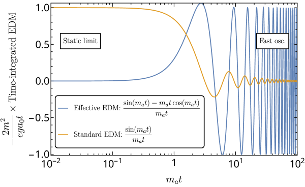
Figure 1: Time-integrated effective EDM including the axion boundary term (blue) vs. standard EDM (yellow), for a constant electric field as given by Eq. (5.15). In the static limit, $m_{a}t\to 0$, the effective EDM vanishes when taking the axion boundary term into account. In the rapidly oscillating regime, $m_{a}t\gg 1$, the axion boundary term dominates and makes the amplitude of the the effective EDM independent of $m_{a}t$, while in contrast the contribution of the standard EDM decouples as $1/(m_{a}t)$.

The behavior of the time-integrated effective EDM of Eq. (5.15) is displayed in Fig. 1, in comparison to the standard EDM contribution discussed e.g. in Ref. [19] (i.e. without axion boundary term).

We conclude that the axion axion boundary term contribution crucially affects the phenomenology of the oscillating EDM, by suppressing the effect in the small oscillation regime and by enhancing it in the fast oscillations domain. Remarkably, for intermediate oscillations the two contributions are comparable, and in the case of an order one axion-electron coupling, as predicted in benchmark axion models [26, 27], the amplitude of the oscillating EDM is of the order of the present static EDM limit. Although static EDM searches cannot be directly employed to set bounds on oscillating EDM scenarios, it is possible that the oscillating nature of this phenomenon could be exploited to gain even larger sensitivities as in the case of oscillating neutron EDM searches [11, 12, 13]. However, a proper discussion of the experimental prospects for measuring such effect is beyond the scope of the present paper and it is left for future work.

6 Conclusions

In this paper, we re-examined the recent claim [19] (see also [20, 21]) that the axion-fermion coupling is responsible for an oscillating EDM in the background of axion dark matter, cf. Eq. (1.1). By employing the Pauli elimination method for the NR expansion of the axion Dirac equation, we provided an alternative derivation of the axion Hamiltonian, emphasizing the equivalence between the derivative and exponential bases.

Unlike previous studies, we pointed out the physical relevance of an axion boundary term, which turns out to be crucial in order to restore the axion shift symmetry and plays a critical role for the oscillating EDM phenomenology, e.g. by leading to an exact cancellation of the standard EDM contribution in the static limit.

In the case of a constant electric field, we were able to introduce the notion of an effective EDM integrated in time, which comprises both the standard contribution of Eq. (1.1) and the axion boundary term. As exemplified by Fig. 1, different patterns emerge depending on the oscillation regime. For slow oscillations, the effective EDM is suppressed compared to the standard one, while for fast oscillations it gets enhanced. In the intermediate oscillations regime instead the effective and standard EDM contributions are comparable.

This new observable is particularly relevant for the case of the electron EDM, since for an $\mathcal{O}(1)$ axion-electron coupling the amplitude of the effective EDM in the intermediate oscillations regime is comparable to the present static EDM limit. The experimental verification of such a scenario remains an interesting open question, which will be addressed elsewhere.

Appendix A Axion Hamiltonian in the exponential basis

Let us consider the exponential basis of Eq. (2.1), in which the axion Dirac equation reads

$$\left(i\gamma^{\mu}\partial_{\mu}-m\,\cos\left(\frac{g\,a}{m}\right)\,+e\gamma^{\mu}A_{\mu}-im\,\sin\left(\frac{g\,a}{m}\right)\,\gamma_{5}\right)\,\psi=0\,.$$ (A.1)

In terms of two-component spinors, as in Eq. (3.4), the axion Dirac equation yields

$$\begin{aligned} \hat{A}&=\hat{\epsilon}+m-m\cos(\frac{g}{m}a)+eA_{0}~{},\\ \hat{B}\,&=\,-\vec{\sigma}\cdot\hat{\vec{P}}-i\,m\,\sin\left(\frac{g\,a}{m}\right)~{},\\ \hat{C}\,&=\,\vec{\sigma}\cdot\hat{\vec{P}}-i\,m\,\sin\left(\frac{g\,a}{m}\right)~{},\\ \hat{D}&=-\left(\hat{\epsilon}+m+m\cos(\frac{g}{m}a)+eA_{0}\right)~{}.\end{aligned}$$ (A.2)

Note that here $\psi=\exp(-i\ m\ t)\ (\chi_{\not{N}},\ \Phi)^{T}$ and $\hat{A},\hat{B},\hat{C}$ and $\hat{D}$ are distinct from their analogs in the derivative basis. Nevertheless, in the interest of simplicity, we will neglect distinguishing subscripts in this appendix. The meaning of the subscript _／N is related to normalization and will become clear later. As in the derivative basis, the Pauli elimination method leads to solutions in the form of Eq. (3.6). Expanding the inverse of $\hat{D}$ in powers of $1/m$, we obtain the same result as Eq. (3.7) at $\mathcal{O}(1/m^{2})$. As in the derivative basis, we match onto the form of a Schrödinger equation, see Eq. (3.8), obtaining the same axion Hamiltonian at $\mathcal{O}(1/m)$ given by Eq. (3.9).

It is worth mentioning that by working in the linear axion basis instead, i.e. approximating $m\cos(ga/m)\simeq ga$ and $m\sin(ga/m)\simeq ga$ in Eq. (A.1), one would have obtained

$$\hat{{\cal H}}^{(1),\,\rm linear}_{a}\,=\,-\frac{g}{2\,m}\vec{\sigma}\cdot\vec{\nabla}a+\frac{g^{2}a^{2}}{2m}~{},$$ (A.3)

featuring a spurious term that breaks the axion shift symmetry. Thus, we stress the importance of properly taking into account the non-linear axion terms arising from the exponential axion parametrization at a given order in the NR expansion.

The previous calculation in the exponential basis can be extended at $\mathcal{O}(1/m^{2})$. From Eq. (3.6) we obtain:

$$i\,\partial_{t}\,\chi_{\not{N}}\,+\,e\,A_{0}\,\chi_{\not{N}}\,-\,\hat{{\cal H}}^{(1)}[\chi_{\not{N}}]\,-\,f^{(2)}(\chi_{\not{N}},\partial_{t}\,\chi_{\not{N}})\,+\,\mathcal{O}(1/m^{3})\,=\,0~{},$$ (A.4)

where $f^{(2)}(\chi_{\not{N}},\partial_{t}\,\chi_{\not{N}})$ is an $\mathcal{O}(1/m^{2})$ function that depends explicitly on $\chi_{\not{N}}$ and $\partial_{t}\,\chi_{\not{N}}$. Note that due to the dependence on $\partial_{t}\,\chi_{\not{N}}$ at $\mathcal{O}(1/m^{2})$, the exponential basis presents a distinct challenge, as it does not allow Eq. (A.4) to be expressed as a Schrödinger-like equation. To eliminate the contribution of $\partial_{t}\,\chi_{\not{N}}$ from this expression we can proceed iteratively, by employing the initial portion of Eq. (A.4),

$$i\,\partial_{t}\,\chi_{\not{N}}\,=\,-\,e\,A_{0}\,\chi_{\not{N}}\,+\,\mathcal{O}(1/m)~{}.$$ (A.5)

Note that there is no need to include here corrections of order $\mathcal{O}(1/m)$ since they will only contribute to the Hamiltonian at order $\mathcal{O}(1/m^{3})$. By performing this iteration, we arrive at the following expression for the Hamiltonian at $\mathcal{O}(1/m^{2})$ in the exponential basis:

$$\hat{{\cal H}}^{(2)}_{a\not{N}}\,=\, -\,\frac{e\,g}{4\,m^{2}}\,a\,\vec{\sigma}\cdot\vec{E}\,-\,\frac{i\,g^{2}}{4\,m^{2}}\,a\,\dot{a}\,-\,\frac{e\,g}{4\,m^{2}}\,\dot{a}\,\vec{\sigma}\cdot\vec{A}-\,\frac{g}{4\,m^{2}}\,\,\dot{a}\,\vec{\sigma}\cdot\hat{\vec{p}}+\,\frac{i\,g}{4\,m^{2}}\,\vec{\sigma}\cdot\vec{\nabla}\dot{a}~{}.$$ (A.6)

In the first term of Eq. (A.6), we see the emergence of an axion-dependent EDM. However, this Hamiltonian features the term $ig^{2}a\dot{a}/(4m^{2})$ which is not Hermitian. This means that if this were to be the actual Hamiltonian, then the normalization of the state would not be preserved in time. This is indeed the meaning of $\chi_{\not{N}}$ and $\hat{{\cal H}}^{(2)}_{a\not{N}}$, whose subscript of which indicates that the field is not correctly normalized.

To address this, consider that the hermiticity of the Dirac Hamiltonian implies that the norm of the state is constant in time, which in coordinate space reads

$$\int\differential[3]{x}\psi^{\dagger}\psi=\text{const}\,.$$ (A.7)

This corresponds to the conservation of the global Noether current, associated with the fermion number, i.e. $\partial_{\mu}(\overline{\psi}\gamma^{\mu}\psi)=0$, from which one obtains the continuity equation $i\partial_{t}(\psi^{\dagger}\psi)=-\vec{\nabla}\cdot(\overline{\psi}\vec{\gamma}\psi)$. Upon integrating the latter equation in $d^{3}x$ one readily obtains Eq. (A.7), which can be also rewritten in terms of the large and small component spinors, i.e.

$$\int\differential[3]{x}\left(\chi_{\not{N}}^{\dagger}\chi_{\not{N}}+\Phi^{\dagger}\Phi\right)\,=\text{const}\,,$$ (A.8)

and substituting $\Phi=-\hat{D}^{-1}[\hat{C}[\chi_{\not{N}}]]$ in the previous equation we obtain

$$\int\differential[3]{x}\psi^{\dagger}\psi=\int\differential[3]{x}\left[\chi_{\not{N}}^{\dagger}\chi_{\not{N}}+\left(\hat{D}^{-1}[\hat{C}[\chi_{\not{N}}]]\right)^{\dagger}\left(\hat{D}^{-1}[\hat{C}[\chi_{\not{N}}]\right)\right].$$ (A.9)

If we were able to reduce Eq. (A.9) to the form

$$\int\differential[3]{x}(\hat{N}[\chi_{\not{N}}])^{\dagger}(\hat{N}[\chi_{\not{N}}])=\int\differential[3]{x}\chi^{\dagger}\chi=\text{const.},$$ (A.10)

then we would have shown that the normalization of the field $\chi=\hat{N}[\chi_{\not{N}}]$ is correctly preserved in time. This is non-trivial to achieve because of the derivative (and thus directional) nature of the operators $\hat{D}^{-1}\hat{C}$. Therefore, we will first evaluate eq. (A.9) in terms of eigenvalues and then seek an operator $\hat{N}$ that produces the same eigenvalues. We thus evaluate $\hat{D}^{-1}[\hat{C}[\chi_{\not{N}}]]=\xi\chi_{\not{N}}$ to find the eigenvalue $\xi$. Explicitly, this is

$$\hat{D}^{-1}[\hat{C}[\chi_{\not{N}}]]=\xi\chi_{\not{N}}=\left(\frac{iag}{2m}-\frac{e\vec{\sigma}\cdot\vec{A}}{2m}-\frac{\vec{\sigma}\cdot\vec{p}}{2m}+\frac{\dot{a}g}{4m^{2}}-\frac{ie\vec{\sigma}\cdot\vec{E}}{4m^{2}}\right)\chi_{\not{N}}+\mathcal{O}\left(\frac{1}{m^{3}}\right),$$ (A.11)

such that $\xi$ no longer contains any derivative acting outside the operator. Here we made the replacement,

$$i\vec{\nabla}\chi_{\not{N}}=-\vec{p}\chi_{\not{N}},$$ (A.12)

and applied Eq. (A.5). In this case, it does not matter in which basis we calculate $\hat{{\cal H}}$ because both the derivative and exponential bases agree to $\mathcal{O}(1/m)$. For this step to be consistent, we have to verify a posteriori that also the Hamiltonian for the normalized spinor agrees up to $\mathcal{O}(1/m)$, which will turn out to be the case. In terms of this eigenvalue $\xi$, we can write

$$\int\differential[3]{x}\tilde{\psi}^{\dagger}\tilde{\psi} =\int\differential[3]{x}\left[\chi_{\not{N}}^{\dagger}\chi_{\not{N}}+\left(\xi\chi_{\not{N}}\right)^{\dagger}\left(\xi\chi_{\not{N}}\right)\right]$$

$$=\int\differential[3]{x}\left[\chi_{\not{N}}^{\dagger}\chi_{\not{N}}+\chi_{\not{N}}^{\dagger}\xi^{\dagger}\xi\chi_{\not{N}}\right]$$

$$=\int\differential[3]{x}\left[\left(N\chi_{\not{N}}\right)^{\dagger}\left(N\chi_{\not{N}}\right)+\mathcal{O}\left(\frac{1}{m^{3}}\right)\right],$$ (A.13)

where we defined the eigenvalue

$$N\equiv 1+\frac{1}{2}\xi^{\dagger}\xi=1+\frac{1}{8m^{2}}\left(a^{2}g^{2}+e^{2}\vec{A}^{2}+\vec{p}^{2}+e\left\{\vec{\sigma}\cdot\vec{p},\vec{\sigma}\cdot\vec{A}\right\}\right)\,.$$ (A.14)

Before promoting $N$ to a proper operator we have to address the last term, because simply promoting $\vec{p}\to\hat{\vec{p}}=-i\vec{\nabla}$ would introduce unintended terms from the resulting product rule. To address this, we can apply the anticommutation rule $\left\{\vec{\sigma}\cdot\vec{x},\vec{\sigma}\cdot\vec{y}\right\}=2\vec{x}\cdot\vec{y}$, such that

$$N\equiv 1+\frac{1}{8m^{2}}\left(a^{2}g^{2}+e^{2}\vec{A}^{2}+\vec{p}^{2}+2e\vec{A}\cdot\vec{p}\right).$$ (A.15)

This is straightforward to promote to an operator form,

$$\hat{N}=1+\frac{1}{8m^{2}}\left(a^{2}g^{2}+e^{2}\vec{A}^{2}+\vec{\nabla}^{2}-2ie\vec{A}\cdot\vec{\nabla}\right),$$ (A.16)

which correctly returns the eigenvalue $N$ when applied to $\chi_{\not{N}}$. By inverting the normalization operator, we finally obtain

$$\hat{N}^{-1}=1-\frac{1}{8m^{2}}\left(a^{2}g^{2}+e^{2}\vec{A}^{2}+\vec{\nabla}^{2}-2ie\vec{A}\cdot\vec{\nabla}\right),$$ (A.17)

such that $\chi_{\not{N}}=\hat{N}^{-1}[\chi]$. Since this operator depends on $a$ it is clear that it introduces corrections also to the axion-dependent part of the Hamiltonian in the exponential basis.

Let us now see if any contributions were missed in the derivative basis. One can proceed similarly and we find the following:

$$\text{Derivative basis:}\quad\hat{N}^{-1}\,=\,1-\frac{1}{8m^{2}}\left(e^{2}\vec{A}^{2}+\vec{\nabla}^{2}-2ie\vec{A}\cdot\vec{\nabla}\right)\ ,$$ (A.18)

where, in contrast to the exponential basis, there is no axion dependence at $\mathcal{O}(1/m^{2})$. This can be clearly seen by inspecting Eq. (3) where the axion contributions enter at $\mathcal{O}(1/m)$ in contrast to Eq. (A.2) where the axion contribution already enters at $\mathcal{O}(1)$. As speculated earlier, this means that the axion-dependent part of the Hamiltonian will not receive any corrections from normalization at $\mathcal{O}(1/m^{2})$ in the derivative basis.

Now that we have identified a spinor that is appropriately normalized, $\chi=\hat{N}[\chi_{\not{N}}]$, we want to derive how the corresponding Hamiltonian is modified. To this end, we rewrite $\hat{{\cal H}}_{\not{N}}[\chi_{\not{N}}]=i\partial_{t}[\chi_{\not{N}}]$ as

$$\hat{{\cal H}}_{\not{N}}[\hat{N}^{-1}[\chi]]=i\partial_{t}[\hat{N}^{-1}[\chi]]~{},$$ (A.19)

and bring this into the canonical form $\hat{H}\chi=i\partial_{t}\chi$. To this end, let us consider the expansions

$$\hat{{\cal H}}_{\not{N}} =\hat{H}_{\not{N}}^{(0)}+\frac{1}{m}\hat{H}_{\not{N}}^{(1)}+\frac{1}{m^{2}}\hat{H}_{\not{N}}^{(2)}+\mathcal{O}(1/m^{3}),$$ (A.20)

$$\hat{N}^{-1} =\hat{\alpha}_{0}+\frac{1}{m}\hat{\alpha}_{1}+\frac{1}{m^{2}}\hat{\alpha}_{2}+\mathcal{O}(1/m^{3}).$$ (A.21)

From Eq. (A.17), we see that $\hat{\alpha}_{0}=1$ and $\hat{\alpha}_{1}=0$ , which verifies our earlier expectations (cf. discussion in footnote 9). Furthermore, we know that normalization only changes terms at $\mathcal{O}(1/m^{2})$, so $\hat{H}_{\not{N}}^{(0)}=\hat{H}^{(0)}$ and $\hat{H}_{\not{N}}^{(1)}=\hat{H}^{(1)}$. In terms of these parameters, Eq. (A.19) becomes

$$i\,\partial_{t}[\chi]=\, \hat{H}^{(0)}[\chi]-\frac{1}{m}\,\hat{H}^{(1)}[\chi]$$

$$-\frac{1}{m^{2}}\,\left(i\,\partial_{t}[\hat{\alpha}_{2}[\chi]]-\hat{H}^{(0)}[\hat{\alpha}_{2}[\chi]]-\hat{H}_{\not{N}}^{(2)}[\chi]\right)+\mathcal{O}(1/m^{3})=0~{}.$$ (A.22)

In Eq. (A) $\hat{\alpha}_{2}$ only appears with $\hat{H}^{(0)}$ which does not contain the axion. Therefore, only the $-a^{2}g^{2}/8$ term from Eq. (A.17) will contribute to the axion-dependent terms at $\mathcal{O}(1/m^{2})$. We then find that

$$\hat{{\cal H}}_{a}^{(2)}[\chi] =\frac{1}{8m^{2}}\left(i\,\partial_{t}[a^{2}g^{2}\chi]-H^{(0)}[a^{2}g^{2}\chi]\right)+\hat{{\cal H}}_{a\not{N}}^{(2)}[\chi]=\frac{ig^{2}}{4m^{2}}a\dot{a}\chi+\hat{{\cal H}}_{a\not{N}}^{(2)}[\chi]\,,$$ (A.23)

which exactly cancels the non-Hermitian term in Eq. (A.6) and yields the axion Hamiltonian in the exponential basis as defined in Eq. (3.12). Note that when we in the main text of this work refer to fields and Hamiltonians defined in the exponential basis we will add the subscript _E to the results above.

References

- [1] R. D. Peccei and H. R. Quinn, “CP Conservation in the Presence of Instantons,” Phys. Rev. Lett. 38 (1977) 1440–1443.
- [2] R. D. Peccei and H. R. Quinn, “Constraints Imposed by CP Conservation in the Presence of Instantons,” Phys. Rev. D16 (1977) 1791–1797.
- [3] S. Weinberg, “A New Light Boson?,” Phys. Rev. Lett. 40 (1978) 223–226.
- [4] F. Wilczek, “Problem of Strong p and t Invariance in the Presence of Instantons,” Phys. Rev. Lett. 40 (1978) 279–282.
- [5] J. Preskill, M. B. Wise, and F. Wilczek, “Cosmology of the Invisible Axion,” Phys. Lett. B 120 (1983) 127–132.
- [6] L. Abbott and P. Sikivie, “A Cosmological Bound on the Invisible Axion,” Phys. Lett. B 120 (1983) 133–136.
- [7] M. Dine and W. Fischler, “The Not So Harmless Axion,” Phys. Lett. B 120 (1983) 137–141.
- [8] L. Di Luzio, M. Giannotti, E. Nardi, and L. Visinelli, “The landscape of QCD axion models,” Phys. Rept. 870 (2020) 1–117, arXiv:2003.01100 [hep-ph].
- [9] I. G. Irastorza and J. Redondo, “New experimental approaches in the search for axion-like particles,” Prog. Part. Nucl. Phys. 102 (2018) 89–159, arXiv:1801.08127 [hep-ph].
- [10] P. Sikivie, “Invisible Axion Search Methods,” Rev. Mod. Phys. 93 no. 1, (2021) 015004, arXiv:2003.02206 [hep-ph].
- [11] P. W. Graham and S. Rajendran, “New Observables for Direct Detection of Axion Dark Matter,” Phys. Rev. D88 (2013) 035023, arXiv:1306.6088 [hep-ph].
- [12] D. Budker, P. W. Graham, M. Ledbetter, S. Rajendran, and A. Sushkov, “Proposal for a Cosmic Axion Spin Precession Experiment (CASPEr),” Phys. Rev. X 4 no. 2, (2014) 021030, arXiv:1306.6089 [hep-ph].
- [13] D. F. Jackson Kimball et al., “Overview of the Cosmic Axion Spin Precession Experiment (CASPEr),” Springer Proc. Phys. 245 (2020) 105–121, arXiv:1711.08999 [physics.ins-det].
- [14] Y. V. Stadnik and V. V. Flambaum, “Axion-induced effects in atoms, molecules, and nuclei: Parity nonconservation, anapole moments, electric dipole moments, and spin-gravity and spin-axion momentum couplings,” Phys. Rev. D 89 no. 4, (2014) 043522, arXiv:1312.6667 [hep-ph].
- [15] C. Abel et al., “Search for Axionlike Dark Matter through Nuclear Spin Precession in Electric and Magnetic Fields,” Phys. Rev. X 7 no. 4, (2017) 041034, arXiv:1708.06367 [hep-ph].
- [16] V. V. Flambaum, M. Pospelov, A. Ritz, and Y. V. Stadnik, “Sensitivity of EDM experiments in paramagnetic atoms and molecules to hadronic CP violation,” Phys. Rev. D 102 no. 3, (2020) 035001, arXiv:1912.13129 [hep-ph].
- [17] S. P. Chang, S. Haciomeroglu, O. Kim, S. Lee, S. Park, and Y. K. Semertzidis, “Axionlike dark matter search using the storage ring EDM method,” Phys. Rev. D 99 no. 8, (2019) 083002, arXiv:1710.05271 [hep-ex].
- [18] O. Kim and Y. K. Semertzidis, “New method of probing an oscillating EDM induced by axionlike dark matter using an rf Wien filter in storage rings,” Phys. Rev. D 104 no. 9, (2021) 096006, arXiv:2105.06655 [hep-ph].
- [19] C. Smith, “On the fermionic couplings of axionic dark matter,” arXiv:2302.01142 [hep-ph].
- [20] S. Alexander and R. Sims, “Detecting axions via induced electron spin precession,” Phys. Rev. D 98 no. 1, (2018) 015011, arXiv:1702.01459 [hep-ph].
- [21] Z. Wang and L. Shao, “Axion induced spin effective couplings,” Phys. Rev. D 103 no. 11, (2021) 116021, arXiv:2102.04669 [hep-ph].
- [22] ACME Collaboration, V. Andreev et al., “Improved limit on the electric dipole moment of the electron,” Nature 562 no. 7727, (2018) 355–360.
- [23] L. L. Foldy and S. A. Wouthuysen, “On the Dirac theory of spin 1/2 particle and its nonrelativistic limit,” Phys. Rev. 78 (1950) 29–36.
- [24] W. Pauli, “Zur Quantenmechanik des magnetischen Elektrons,” Zeitschrift für Physik 43 no. 9-10, (1927) 601–623.
- [25] E. de Vries and J. E. Jonker, “Non-relativistic approximations of the Dirac Hamitonian,” Nucl. Phys. B 6 (1968) 213–225.
- [26] A. R. Zhitnitsky, “On Possible Suppression of the Axion Hadron Interactions. (In Russian),” Sov. J. Nucl. Phys. 31 (1980) 260. [Yad. Fiz.31,497(1980)].
- [27] M. Dine, W. Fischler, and M. Srednicki, “A Simple Solution to the Strong CP Problem with a Harmless Axion,” Phys. Lett. B104 (1981) 199–202.
- [28] K. Fujikawa, “Path Integral Measure for Gauge Invariant Fermion Theories,” Phys. Rev. Lett. 42 (1979) 1195–1198.
- [29] W. Pauli, Die Allgemeinen Prinzipien der Wellenmechanik. Springer, Berlin, Germany, Nov., 1990.
- [30] M. Pospelov, A. Ritz, and M. B. Voloshin, “Bosonic super-WIMPs as keV-scale dark matter,” Phys. Rev. D 78 (2008) 115012, arXiv:0807.3279 [hep-ph].
- [31] R. Shankar, Principles of Quantum Mechanics. Springer, 1994. https://books.google.it/books?id=2zypV5EbKuIC.
- [32] S. Kamefuchi, L. O’Raifeartaigh, and A. Salam, “Change of variables and equivalence theorems in quantum field theories,” Nucl. Phys. 28 (1961) 529–549.
- [33] J. S. R. Chisholm, “Change of variables in quantum field theories,” Nucl. Phys. 26 no. 3, (1961) 469–479.
- [34] R. E. Kallosh and I. V. Tyutin, “The Equivalence theorem and gauge invariance in renormalizable theories,” Yad. Fiz. 17 (1973) 190–209.
- [35] Particle Data Group Collaboration, R. L. Workman et al., “Review of Particle Physics,” PTEP 2022 (2022) 083C01.