2023 188 28 August

Semi-inclusive h+jet production in $\mathrm{pp}$ and Pb–Pb collisions ALICE Collaboration ALICE Collaboration

The ALICE Collaboration reports measurements of the semi-inclusive distribution of charged-particle jets recoiling from a high transverse momentum (high $p_{\mathrm{T}}$) charged hadron, in $\mathrm{pp}$ and central Pb–Pb collisions at center of mass energy per nucleon–nucleon collision $\sqrt{s_{\mathrm{NN}}}=5.02$ TeV. The large uncorrelated background in central Pb–Pb collisions is corrected using a data-driven statistical approach, which enables precise measurement of recoil jet distributions over a broad range in $p_{\mathrm{T,ch~{}jet}}$ and jet resolution parameter $R$. Recoil jet yields are reported for $R=0.2$, 0.4, and 0.5 in the range $7<p_{\mathrm{T,ch~{}jet}}<140$ $\mathrm{GeV/}c$ and $\pi/2<\Delta\varphi<\pi$, where $\Delta\varphi$ is the azimuthal angular separation between hadron trigger and recoil jet. The low $p_{\mathrm{T,ch~{}jet}}$ reach of the measurement explores unique phase space for studying jet quenching, the interaction of jets with the quark–gluon plasma generated in high-energy nuclear collisions. Comparison of $p_{\mathrm{T,ch~{}jet}}$ distributions from $\mathrm{pp}$ and central Pb–Pb collisions probes medium-induced jet energy loss and intra-jet broadening, while comparison of their acoplanarity distributions explores in-medium jet scattering and medium response. The measurements are compared to theoretical calculations incorporating jet quenching.

1 Introduction

Nuclear matter under conditions of extreme temperature and pressure forms a quark–gluon plasma (QGP), the deconfined state of matter whose dynamics are governed by interactions between sub-hadronic constitutents [1, 2]. The QGP filled the early universe a few microseconds after the Big Bang, and is generated and studied today using collisions of atomic nuclei at the CERN Large Hadron Collider (LHC) and the Brookhaven Relativistic Heavy Ion Collider (RHIC). Experimental measurements at these facilities, together with their comparison to theoretical calculations, have shown that the QGP is a fluid with very low specific viscosity [3, 4, 5, 6] that is opaque to the passage of energetic color charges [7, 8].

In hadronic collisions, jets arise in hard (high-momentum-transfer ${Q}^{2}$) interactions of quarks and gluons (partons) from the projectiles. The scattered partons are initially virtual and come on-shell through gluon radiation, which generates a parton shower. The shower subsequently hadronizes, and the jet can be observed in a detector as a collimated spray of hadrons. Jet reconstruction algorithms have been developed which apply both to experimental data and to theoretical calculations based on perturbative quantum chromodynamics (pQCD), providing well-controlled theory/data comparisons [9]. Jet production and substructure have been measured extensively in proton–proton ($\mathrm{pp}$) collisions, and pQCD calculations are found to be in excellent agreement with such measurements over a wide kinematic range [10, 11, 12, 13, 14, 15, 16, 17, 18, 19, 20, 21]. Jets in $\mathrm{pp}$ collisions therefore provide incisive probes of QCD.

In heavy-ion collisions at collider energies, jets are generated concurrently with the QGP. Following a high-${Q}^{2}$ partonic interaction, the evolving parton shower interacts with the expanding and cooling QGP. These secondary interactions proceed via elastic (collisional) and inelastic (radiative) processes, which modify jet production and structure relative to jets generated in vacuum (“jet quenching”). Experimentally observable consequences of jet quenching include energy transport out of the jet cone (energy loss); modification of intra-jet structure; and jet deflection. Extensive jet quenching measurements have been carried out with nuclear collisions at RHIC and the LHC (see [7, 8, 22, 23] and references therein).

The measurement of reconstructed jets in heavy-ion collisions is challenging, however, due to the large background in the complex environment of such collisions. Initial studies of jet quenching therefore utilized high-$p_{\mathrm{T}}$ hadron production and correlations  [24, 25, 26, 27, 28, 29, 30, 31, 32, 33], which are more readily measurable with high precision in such an environment. High-$p_{\mathrm{T}}$ hadrons are leading fragments of jets, and inclusive high-$p_{\mathrm{T}}$ hadron yield suppression is the hallmark of partonic energy loss due to jet quenching. Comparison of inclusive hadron suppression data with theoretical models has been used to constrain the in-medium jet transport parameter $\hat{q}$, which characterizes the magnitude of energy loss in jet quenching models [34, 35, 36, 37, 38, 39, 40, 41, 42]. However, observed high-$p_{\mathrm{T}}$ hadrons are expected to arise predominantly from jets which experience relatively little medium-induced energy loss, due to the interplay of the steeply falling inclusive jet energy spectrum shape, the hadron fragmentation function, and energy loss [43, 44, 45, 46]. Deeper insight into the mechanisms underlying jet quenching and the response of the QGP to the passage of energetic partons requires measurements incorporating reconstructed jets.

Significant progress has been made over the past decade in the measurement of reconstructed jets in heavy-ion collisions in terms of inclusive jet production, di-jet correlations, and trigger–jet coincidence observables [47, 48, 49, 50, 51, 52, 53, 54, 55, 17, 56, 57, 58, 59, 60, 61, 62, 63, 64, 65, 66, 67, 68, 69, 70, 71, 72]. Model studies incorporate both jet and hadronic observables, for a more comprehensive study of jet quenching (e.g. [73, 8, 74]).

In this manuscript and its companion Letter [75], the ALICE Collaboration reports new measurements of the semi-inclusive distribution of charged-particle jets recoiling from a high-$p_{\mathrm{T}}$ hadron (“h+jet”)  [50, 70, 53] in $\mathrm{pp}$ and central Pb–Pb collisions at center-of-mass energy per nucleon–nucleon collision $\sqrt{s_{\mathrm{NN}}}=5.02$ TeV. The analysis utilizes the approach developed in Ref. [50], which provides data-driven correction of the complex uncorrelated background for jet measurements in central collisions of nuclei (A–A). This approach enables systematically well-controlled jet measurements over a broad range, including low jet transverse momentum ($p_{\mathrm{T,jet}}$) and large resolution parameter $R$. These measurements extend significantly the $p_{\mathrm{T,jet}}$ reach at both high and low $p_{\mathrm{T,jet}}$ relative to that in Ref. [50], down to the lowest $p_{\mathrm{T,jet}}$ values that are interpretable in terms of perturbatively generated jets ($p_{\mathrm{T,jet}}\sim 10$ $\mathrm{GeV/}c$; see also [70]).

Corrected semi-inclusive recoil jet yields measured in $\mathrm{pp}$ and central Pb–Pb collisions are compared, in order to explore jet quenching. The $R$ and $p_{\mathrm{T,jet}}$-dependence of recoil yields is reported, which is sensitive to jet energy loss and medium-induced intra-jet broadening [50, 70, 71, 17]. Distributions in $\Delta\varphi$, the trigger–recoil jet azimuthal separation (acoplanarity), are also reported, which probe in-medium multiple scattering [76, 77, 78], scattering from QGP quasi-particles [79, 80], or the response of the QGP medium to energy loss [35, 81, 82]. The measurements are also compared to theoretical models incorporating jet quenching.

The low $p_{\mathrm{T,jet}}$ reach of this measurement, which to date is unique for reconstructed jet measurements in heavy-ion collisions at the LHC, is notable. Jet measurements in heavy-ion collisions, which impose a lower threshold in jet $p_{\mathrm{T}}$ of a few 10s of $\mathrm{GeV/}c$, are subject to a selection bias in the reported jet population (for instance, in the relative fraction of quark and gluon jets), which complicates their interpretation in terms of jet quenching [83, 84]. The measurements reported here are much less affected by this bias, however, because of their much lower $p_{\mathrm{T,jet}}$ threshold. For acoplanarity measurements, low $p_{\mathrm{T,jet}}$ is advantageous because medium-induced effects are expected to be largest in relative terms in that range, and in-vacuum broadening due to Sudakov radiation is smallest at low $p_{\mathrm{T,jet}}$ [76].

These measurements at low $p_{\mathrm{T,jet}}$ and large $R$ in Pb–Pb collisions require the determination of a trigger-correlated signal in a large and complex background. This paper details the data-driven procedures used to carry out such measurements and determine their uncertainties. However, it is also valuable to carry out a qualitative cross-check of the entire framework, to ascertain the degree to which the correlated signal reported at low $p_{\mathrm{T,jet}}$ and large $R$ is already present in the raw data, prior to application of the correction procedures, and is not generated solely by the corrections. This cross-check is also presented.

The manuscript is organized as follows: Sec. 2 presents the detector and datasets; Sec. 3 presents the analysis algorithms and observables; Sec. 4 and 5 present the raw distributions in Pb–Pb and $\mathrm{pp}$ collisions, respectively; Sec. 6 presents the theoretical models and simulations used for correction of the data and for physics studies; Sec. 7 presents the correction procedures; Sec. 8 presents the systematic uncertainties; Sec. 9 presents the closure test for the Pb–Pb analysis; Sec. 10 presents the results; and Sec. 11 presents a summary and outlook.

2 Detector and datasets

The ALICE experiment and its performance are described in Refs. [85, 86]. The ALICE central barrel consists of detectors for charged-particle tracking, particle identification, and electromagnetic calorimetry, inside a large solenoidal magnet a with field strength of 0.5 T. The tracking in this analysis is carried out by the Inner Tracking System (ITS) [87], a 6-layer silicon detector with radial distance 3.9–43 cm from the beamline, and the Time Projection Chamber (TPC) [88], a gaseous detector with radial distance 85–247 cm from the beamline. Both detectors provide precise charged-particle tracking for track $p_{\mathrm{T}}>0.2$ $\mathrm{GeV/}c$ within a pseudorapidity ($\eta$) coverage of $\eta<0.9$.

2.1 Datasets

Online triggering for the datasets used in this analysis was based on signals in the V0A and V0C forward scintillation detectors [89], collectively referred to as V0. The V0A acceptance is $2.8<\eta<5.1$ and that of V0C is $-3.7<\eta<-1.7$, over the full azimuth.

pp data:

The data used in this analysis for $\mathrm{pp}$ collisions at $\sqrt{s}=5.02$ TeV were recorded during the 2015 and 2017 LHC running periods, with a minimum bias (MB) trigger that required a coincidence signal in V0A and V0C.

Offline event selection requires the presence of a primary vertex constructed from at least two tracklets, which are track segments formed by pairing hits in the Silicon Pixel Detector (SPD), the two layers of the ITS which are closest to the beam line; a primary vertex formed by tracks from the full tracking system with position in the beam direction $|z_{\mathrm{vtx}}^{\mathrm{track}}|<10$ cm relative to the nominal center of ALICE; and consistency in the location of the two vertices, $|z_{\mathrm{vtx}}^{\mathrm{track}}-z_{\mathrm{vtx}}^{\mathrm{SPD}}|<0.5$ cm. In-bunch event pileup is suppressed by rejecting events where multiple vertices are reconstructed, while out-of-bunch pileup is rejected based on V0 timing.

After event selection cuts, 100M $\mathrm{pp}$ collision events from the 2015 data taking period and 940M events from the 2017 data taking period are accepted. Detailed study of the features of the two datasets finds excellent consistency. They are combined and analyzed together, leading to a total of 1.04B $\mathrm{pp}$ events which corresponds to an integrated luminosity of $20$ $\mathrm{nb^{-1}}$.

Pb–Pb  data:

The data used in this analysis for Pb–Pb collisions at $\sqrt{s_{\mathrm{NN}}}=5.02$ TeV were recorded during the 2018 LHC heavy-ion run. Minimum-bias events were triggered online based on the coincidence of signals in the V0A and V0C detectors. A separate trigger class based on the V0 signal amplitude was used to collect a larger sample of central Pb–Pb collisions. Offline event selection requires $|z_{\mathrm{vtx}}^{\mathrm{track}}|<10$ cm relative to the nominal center of ALICE. Same-bunch collision pileup is negligible in the Pb–Pb sample, while out-of-bunch pileup within the SPD readout time was removed using V0 timing information. Additional selection based on the correlation between the number of SPD tracklets and the number of TPC clusters was applied, to suppress pileup of collisions from different bunch crossings that occur within the TPC readout time [86].

Events are characterized offline by “centrality,” which is defined in terms of the percentile of the Pb–Pb hadronic cross section using the summed V0A and V0C (V0) signal amplitudes [90]. The Pb–Pb analysis focuses on “central” collisions, corresponding to 10% of the Pb–Pb hadronic cross section with the largest V0 signal amplitude. After event selection, the central Pb–Pb dataset comprises 89M events, corresponding to an integrated luminosity of $0.12$ $\mathrm{nb^{-1}}$.

2.2 Track reconstruction

Charged-particle tracking is performed offline using hits in the ITS and TPC, both covering $|\eta|<0.9$ over the full azimuth. The SPD had spatially non-uniform and time-varying coverage during the recording of these data. In order to ensure uniform and stable tracking efficiency in the analysis, “hybrid” tracks are therefore employed for both the $\mathrm{pp}$ and Pb–Pb analyses. The hybrid track population consists of two exclusive sets of tracks: “global tracks”, which are tracks with at least one SPD hit and good track-fit residuals in the ITS, but without a primary vertex constraint; and “complementary” tracks, which do not have any SPD hits, are constrained by the primary vertex, and likewise have good track-fit residuals in the ITS. Both sets of tracks are required to have at least 70 crossed pad rows and at least 80% of the geometrically findable space-points in the TPC. Tracks accepted for the analysis have $|\eta|<0.9$ over the full azimuth, and transverse momentum of $p_{\mathrm{T}}>0.15$ $\mathrm{GeV/}c$.

The tracking efficiency is estimated from a full detector simulation. For $\mathrm{pp}$ collisions, the tracking efficiency is 60% for $p_{\mathrm{T}}=0.15$ $\mathrm{GeV/}c$, increasing to 80% for $p_{\mathrm{T}}>0.4$ $\mathrm{GeV/}c$ [56]. For central Pb–Pb collisions, the tracking efficiency is lower than that in $\mathrm{pp}$ collisions by up to 2%. The momentum resolution in $\mathrm{pp}$ collisions is better than 3% for hybrid tracks for $p_{\mathrm{T}}<1$ $\mathrm{GeV/}c$, increasing linearly to 10% at $p_{\mathrm{T}}=100$ $\mathrm{GeV/}c$ [86]. In central Pb–Pb collisions, the momentum resolution worsens by $10-15$% at high $p_{\rm T}$ relative to the momentum resolution in $\mathrm{pp}$ due to the high-multiplicity environment.

3 Analysis

The analysis strategy and procedures are based on those developed in Ref. [50]. Their main features are discussed in this section.

3.1 Event selection

Event selection requires the presence of a high-$p_{\mathrm{T}}$ charged-hadron trigger particle in a defined $p_{\mathrm{T}}$ interval, $p_{\mathrm{T,low}}<p_{\mathrm{T}}^{\mathrm{trig}}<p_{\mathrm{T,high}}$ $\mathrm{GeV/}c$, denoted $\mathrm{TT}\{p_{\mathrm{T,low}},p_{\mathrm{T,high}}\}$ (“Trigger Track”). If an event contains more than one hadron in the trigger interval, one is chosen at random. With this definition, the $p_{\mathrm{T}}$ dependence of the TT population is the same as that of the inclusive charged-hadron yield distribution.

The principal analysis is carried out using charged-hadron triggers in $\mathrm{TT}\{20,50\}$(signal distribution, denoted $\mathrm{TT}_{\mathrm{sig}}$). Uncorrelated background yield is corrected using a lower-$p_{\mathrm{T}}^{\mathrm{trig}}$ interval, corresponding to $\mathrm{TT}\{5,7\}$ (reference distribution, denoted $\mathrm{TT}_{\mathrm{ref}}$; see Sec. 3.4). The Pb–Pb and $\mathrm{pp}$ datasets are each divided randomly into two distinct subsets of unequal numbers of events, with one for selecting the $\mathrm{TT}_{\mathrm{sig}}$ population and the other for $\mathrm{TT}_{\mathrm{ref}}$. The relative fraction of the population in each subset is chosen to maximize the statistical precision of the corrected distributions. For the Pb–Pb dataset, 95% of events are assigned to the $\mathrm{TT}_{\mathrm{sig}}$ population and 5% are assigned to the $\mathrm{TT}_{\mathrm{ref}}$ population, while for the $\mathrm{pp}$ dataset the corresponding fractions are 90% and 10%.

3.2 Jet reconstruction

Several types of jets are used in the analysis, which are distinguished by labelling their assigned $p_{\mathrm{T}}$ as follows [50]:

• For real data, $p_{\mathrm{T,ch~{}jet}}^{\mathrm{raw}}$ refers to the raw output of the jet-reconstruction algorithm; $p_{\mathrm{T,ch~{}jet}}^{\mathrm{reco}}$ denotes $p_{\mathrm{T,ch~{}jet}}^{\mathrm{raw}}$ after event-wise subtraction for the uncorrelated background energy (Eq. 3); and $p_{\mathrm{T,ch~{}jet}}$ denotes $p_{\mathrm{T}}$ for fully corrected jet distributions.

• For simulations, $p_{\mathrm{T,ch~{}jet}}^{\mathrm{part}}$ refers to jets reconstructed from generated charged particles (particle level), and $p_{\mathrm{T,ch~{}jet}}^{\mathrm{det}}$ refers to jets built from reconstructed charged tracks from the simulated data (detector level);

• Generic reference to a jet without specification of its level of correction or simulation is denoted $p_{\mathrm{T,jet}}$.

The measured distributions are two-dimensional functions of $p_{\mathrm{T,ch~{}jet}}$ and $\Delta\varphi$, so the same labelling likewise applies to $\Delta\varphi$ distributions. However, for simplicity the jet type label (reco, part, or det) of the $\Delta\varphi$ distributions is suppressed and can be deduced from context.

Jet reconstruction is carried out on TT-selected events. Jet reconstruction for both $\mathrm{pp}$ and Pb–Pb collisions is performed using charged-particle tracks with $|\eta|<0.9$ and $p_{\mathrm{T}}>0.15$ $\mathrm{GeV/}c$ over the full azimuth, using the Fastjet implementation of the $k_{\mathrm{T}}$ and anti-$k_{\mathrm{T}}$ algorithms with boost-invariant $p_{\mathrm{T}}$-recombination scheme [91, 92, 9]. The momentum resolution is limited for high-$p_{\mathrm{T}}$ tracks, and jet candidates containing a track constituent with $p_{\mathrm{T}}>100$ $\mathrm{GeV/}c$ are rejected. Less than 1% of jet candidates in the range $100<p_{\mathrm{T,ch~{}jet}}^{\mathrm{reco}}<140$ $\mathrm{GeV/}c$ are rejected by this cut, with negligible effect on the corrected physics distributions.

For both collision systems, jet reconstruction is carried out twice on each event. The first reconstruction pass utilizes the $k_{\mathrm{T}}$ algorithm and accepts jets with $|\eta_{\mathrm{jet}}|<0.9-R$, where $\eta_{\mathrm{jet}}$ is the jet centroid calculated by the $p_{\mathrm{T}}$-weighted vector sum of its constituent momenta. The first-pass jet population is used to determine $\rho$, the event-wise estimate of the background energy density [93]. For Pb–Pb collisions, $\rho$ is defined as

$$\rho=\mathrm{median}\left\{\frac{p_{\mathrm{T,ch~{}jet}}^{\mathrm{raw,}i}}{A_{\mathrm{jet}}^{i}}\right\},$$ (1)

where $p_{\mathrm{T,ch~{}jet}}^{\mathrm{raw,}i}$ and $A_{\mathrm{jet}}^{i}$ are the raw (uncorrected) jet $p_{\mathrm{T}}$ and area [94] of the $i^{\mathrm{th}}$ jet in the event, respectively. Jet area is calculated using ghosts with area 0.005 [94]. For $\mathrm{pp}$ collisions a modified definition appropriate for sparse events [95] is utilized.

$$\rho=C\times\mathrm{median}\left\{\frac{p_{\mathrm{T,ch~{}jet}}^{\mathrm{raw,}i}}{A_{\mathrm{jet}}^{i}}\right\};\ \ C=\frac{\sum_{i}A_{\mathrm{jet}}^{i}}{A_{\mathrm{total}}},$$ (2)

in which $i$ enumerates reconstructed jet candidates, and $A_{\mathrm{total}}=1.8\times 2\pi$ corresponds to the total detector acceptance. The two hardest jets in the event are excluded from the median calculation [93] in both Eq. 1 and 2.

The second jet reconstruction pass utilizes the anti-$k_{\mathrm{T}}$ algorithm  [9] with $R=0.2,0.4$, and $0.5$. The jet centroid is likewise calculated as the $p_{\mathrm{T}}$-weighted vector sum of constituents, with acceptance $|\eta_{\mathrm{jet}}|<0.9-R$ over the full azimuth. An additional selection on the jet area is applied to suppress unphysical jet candidates [50], requiring that $A_{\mathrm{jet}}>0.07$ for $R=0.2$, $A_{\mathrm{jet}}>0.4$ for $R=0.4$, and $A_{\mathrm{jet}}>0.6$ for $R=0.5$.

The raw jet $p_{\mathrm{T}}$ is then corrected event-wise for the estimated background density $\rho$ according to [93]

$$p_{\mathrm{T,ch~{}jet}}^{\mathrm{reco,}i}=p_{\mathrm{T,ch~{}jet}}^{\mathrm{raw,}i}-\rho A_{\mathrm{jet}}^{i},$$ (3)

where $\rho$ for the event is calculated using either Eq. 1 or 2. This adjustment accounts largely for event-wise variation in the overall level of background, which can be sizable for central Pb–Pb collisions due to the broad distribution of charged-particle multiplicity within the $0-10$% centrality class. However, it does not account for local background fluctuations, which likewise are sizable. Such residual fluctuations are corrected by unfolding ensemble-level distributions, as discussed in Sec. 7.

3.3 Semi-inclusive distributions

For each TT-selected event set, recoil jet candidates are tabulated in bins of $p_{\mathrm{T,ch~{}jet}}^{\mathrm{reco}}$ and $\Delta\varphi$, and the distribution is normalized to the number of triggers $N_{\mathrm{trig}}$. This normalized distribution is semi-inclusive, since event selection is based solely upon the presence of an inclusively-distributed high-$p_{\mathrm{T}}$ trigger track, without requiring the presence of jets with specific properties in the recoil region. It is therefore equivalent to the ratio of hard cross sections [50],

$$\frac{1}{N_{\mathrm{trig}}}\frac{\mathrm{d}{{}^{2}}N_{\mathrm{jet}}^{\mathrm{corr}}}{\mathrm{d}p_{\mathrm{T,jet}}\mathrm{d}\Delta\varphi}\Bigg{|}_{p_{\mathrm{T}}^{\mathrm{trig}}\in{\mathrm{TT}}}=\left(\frac{1}{\sigma^{\mathrm{AA}\rightarrow{\mathrm{h}}}}\frac{\rm{d}^{2}\sigma^{\mathrm{AA}\rightarrow{\mathrm{h+jet}}}}{\mathrm{d}p_{\mathrm{T,jet}}\mathrm{d}\Delta\varphi}\right)\Bigg{|}_{p_{\mathrm{T,h}}\in{\mathrm{TT}}},$$ (4)

where $\mathrm{d}{{}^{2}}N_{\mathrm{jet}}^{\mathrm{corr}}/\mathrm{d}p_{\mathrm{T,jet}}\mathrm{d}\Delta\varphi$ represents the differential yield of recoil jets, AA denotes $\mathrm{pp}$ or Pb–Pb collisions, $\sigma^{\mathrm{AA}\rightarrow{\mathrm{h}}}$ is the cross section to generate a hadron within the $p_{\mathrm{T}}$ interval of the selected TT class, and $\mathrm{d}^{2}\sigma^{\mathrm{AA}\rightarrow{\mathrm{h+jet}}}/\mathrm{d}p_{\mathrm{T,jet}}\mathrm{d}\Delta\varphi$ is the differential cross section for coincidence production of a hadron in the TT interval and a recoil jet. Both cross sections in the ratio are perturbatively calculable in $\mathrm{pp}$ collisions [96, 50].

In central Pb–Pb collisions, the measured recoil jet population contains correlated jet candidates that originate from the same high-${Q}^{2}$ interaction as the trigger track. In addition, the population contains uncorrelated combinatorial jet candidates arising from the random overlap of hadrons originating from multiple soft (low-${Q}^{2}$) interactions, and uncorrelated but physical jet candidates arising from a different high-${Q}^{2}$ interaction than the trigger (multi-partonic interactions) [50, 70]. The uncorrelated yield can be sizable, especially for jets with large $R$ at low $p_{\mathrm{T,jet}}$ in central Pb–Pb collisions.

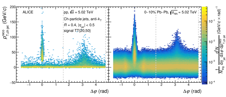
Figure 1: Trigger-normalized recoil jet distributions ($R=0.4$) as a function of $\Delta\varphi$ and $p_{\mathrm{T,ch~{}jet}}^{\mathrm{reco}}$, in $\mathrm{pp}$ collisions (left) and in Pb–Pb collisions (right) at $\sqrt{s_{\mathrm{NN}}}=5.02$ TeV, for $\mathrm{TT}\{20,50\}$ $\mathrm{GeV/}c$. The azimuthal region of the analysis is indicated by the vertical dashed lines.

Figure 1 shows the trigger-normalized recoil jet distributions for $\mathrm{TT}\{20,50\}$ in $\mathrm{pp}$ (left panel) and central Pb–Pb (right panel) collisions for $R=0.4$. While the distributions are displayed over the full range in $\Delta\varphi$, this analysis focuses on the recoil region $\pi/2<\Delta\varphi<3\pi/2$, as indicated by the vertical dashed lines. In Pb–Pb collisions there is significant yield in the region $p_{\mathrm{T,ch~{}jet}}^{\mathrm{reco}}<0$. This yield arises because $\rho$ is the median jet $p_{\mathrm{T}}$-density in the event, i.e. approximately half of the acceptance has local $p_{\mathrm{T}}$-density less than $\rho$. As discussed in Refs. [50, 70], this yield originates predominantly from background fluctuations and enables data-driven normalization of background yield. This population is therefore not rejected; all jet candidates are accepted in the analysis.

3.4 Definition of the $\boldsymbol{\Delta_{\mathrm{recoil}}}$ observable

The goal of this analysis is to measure the trigger-normalized recoil jet distribution over a broad phase space, including low $p_{\mathrm{T,jet}}$ and large $R$. However, in practice the semi-inclusive yield contains both trigger-correlated and uncorrelated contributions to the recoil jet yield. Uncorrelated background yield is especially large relative to correlated signal for low $p_{\mathrm{T,jet}}$ and large $R$ in central Pb–Pb collisions. The uncorrelated background distribution cannot be modeled accurately, and well-controlled background correction requires a fully data-driven approach.

The choice of observable for this analysis is motivated by the observation that, by definition, the trigger-normalized uncorrelated jet yield is independent of $p_{\mathrm{T}}^{\mathrm{trig}}$, and can therefore be removed by subtracting trigger-normalized recoil jet yields obtained with two different TT ranges. The observable $\Delta_{\mathrm{recoil}}$ [50], which is designed for this purpose, is the difference between two semi-inclusive distributions with widely differing $p_{\mathrm{T}}^{\mathrm{trig}}$ ranges: the signal distribution, denoted $\mathrm{TT}_{\mathrm{sig}}$, and the reference distribution, denoted $\mathrm{TT}_{\mathrm{ref}}$,

$$\Delta_{\mathrm{recoil}}(p_{\mathrm{T,jet}},\Delta\varphi)=\frac{1}{N_{\mathrm{trig}}}\frac{{\rm d}^{2}N_{\mathrm{jet}}}{{\mathrm{d}p_{\mathrm{T,jet}}}{\mathrm{d}\Delta\varphi}}\Bigg{|}_{p_{\mathrm{T}}^{\mathrm{trig}}\in{\mathrm{TT}_{\mathrm{sig}}}}-c_{\mathrm{Ref}}\times\frac{1}{N_{\mathrm{trig}}}\frac{{\rm d}^{2}N_{\mathrm{jet}}}{{\mathrm{d}p_{\mathrm{T,jet}}}{\mathrm{d}\Delta\varphi}}\Bigg{|}_{p_{\mathrm{T}}^{\mathrm{trig}}\in{\mathrm{TT}_{\mathrm{ref}}}},$$ (5)

where $c_{\mathrm{Ref}}$ is a normalization factor whose value is determined from the data. Scaling the $\mathrm{TT}_{\mathrm{ref}}$ distribution by $c_{\mathrm{Ref}}$ is needed to account for the effect of the correlated recoil jet yield at large positive $p_{\mathrm{T,ch~{}jet}}^{\mathrm{reco}}$, which is smaller in the $\mathrm{TT}_{\mathrm{ref}}$ population, on the magnitude of the normalized distribution at small and negative $p_{\mathrm{T,ch~{}jet}}^{\mathrm{reco}}$ [50] (see also Sec. 4.2). The $\Delta_{\mathrm{recoil}}(p_{\mathrm{T,jet}},\Delta\varphi)$ is normalized to unit $\eta_{\mathrm{jet}}$ (notation not shown).

While the subtraction in $\Delta_{\mathrm{recoil}}$ removes the large uncorrelated jet yield, the $\mathrm{TT}_{\mathrm{ref}}$ population contains an admixture of trigger-correlated yield which is also removed from the measurement by the subtraction. As noted in Sec. 3.1, the $\mathrm{TT}_{\mathrm{ref}}$ $p_{\mathrm{T}}$-range is $\mathrm{TT}\{5,7\}$. This $p_{\mathrm{T}}$-interval is chosen to minimize the $\mathrm{TT}_{\mathrm{ref}}$ correlated component, while still having high enough trigger $p_{\mathrm{T}}$ that its inclusive production cross section is perturbatively calculable in $\mathrm{pp}$ collisions. The $\Delta_{\mathrm{recoil}}$ distribution is therefore not that of a single semi-inclusive recoil distribution, but rather the difference of two such distributions, both of which are perturbatively calculable; the $\Delta_{\mathrm{recoil}}$ distribution is likewise perturbatively calculable.

In order to assess the effect of the subtraction of the $\mathrm{TT}_{\mathrm{ref}}$ correlated yield for the choice $\mathrm{TT}_{\mathrm{ref}}=\mathrm{TT}\{5,7\}$, the analysis was also carried out with $\mathrm{TT}_{\mathrm{ref}}=\mathrm{TT}\{8,9\}$. While small differences are observed in the central values of the corrected results, all such differences are smaller than the systematic uncertainties of the measurement. This variation is however not an uncertainty; the choice of $\mathrm{TT}_{\mathrm{ref}}$ defines the observable. This cross-check shows rather that the physics conclusions from the analysis are not significantly dependent upon the specific choice of $\mathrm{TT}_{\mathrm{ref}}$.

This manuscript reports the following projections of $\Delta_{\mathrm{recoil}}(p_{\mathrm{T,jet}},\Delta\varphi)$:

• $\Delta_{\mathrm{recoil}}(p_{\mathrm{T,jet}})$: projection onto $p_{\mathrm{T,jet}}$ for $|\Delta\varphi-\pi|<0.6$;

• $\Delta_{\mathrm{recoil}}(\Delta\varphi)$: projection onto $\Delta\varphi$ for various intervals in $p_{\mathrm{T,jet}}$.

4 Measurement of $\Delta_{\mathrm{recoil}}$: central Pb–Pb collisions

For jet measurements in central Pb–Pb collisions at low $p_{\mathrm{T,jet}}$ and large $R$, where the uncorrelated background is much larger than the correlated signal yield, the two terms in Eq. 5 are similar in magnitude. Measurement of the correlated signal in this region therefore requires accurate determination of a small difference between two large numbers. This in turn requires precise relative calibration of the two terms, for both $p_{\mathrm{T}}$-scale and yield.

This calibration is based on the observation, discussed above, that the jet yield in the region $p_{\mathrm{T,ch~{}jet}}^{\mathrm{reco}}<0$ is strongly dominated by background fluctuations, whose contribution is common to the two terms in Eq. 5.

Specifically, the calibrated distributions of the two terms in Eq. 5 are required to be consistent within statistical uncertainties over a significant range in the left-most part of the $p_{\mathrm{T,ch~{}jet}}^{\mathrm{reco}}$ distribution [50, 70]. As shown in Fig. 3, the distributions vary significantly in this region; this requirement is therefore highly restrictive, providing strong and purely data-driven constraints on the calibration.

4.1 Relative $\mathbf{p_{\mathrm{T}}}$-scale calibration: $\Delta\mathbf{\rho}$

The two terms in Eq. 5 correspond to different TT-selected populations, which have significantly different recoil jet $p_{\mathrm{T}}$ spectra (Figs. 3 and 8). Since the presence of correlated hard jets reduces the acceptance for uncorrelated, soft combinatorial jets [50], this difference can generate different $\rho$ distributions (Eq. 1) [70]. This in turn will affect the $p_{\mathrm{T}}$-scale calibration, since Eq. 5 is a function of $p_{\mathrm{T,ch~{}jet}}^{\mathrm{reco}}$, which includes the area-based adjustment $\rho A_{\mathrm{jet}}$ (Eq. 3).

In Ref. [70], comparison of the $\rho$ distributions in the same event (SE) and mixed event (ME) populations shows that their shapes are similar but are displaced by a shift $\Delta\rho=60$ MeV/$c$. Shifting the ME $\rho$ distribution by $\Delta\rho=60$ MeV/$c$ significantly improves the agreement of the shapes of the SE and ME $p_{\mathrm{T,ch~{}jet}}^{\mathrm{reco}}$ distributions in the region $p_{\mathrm{T,ch~{}jet}}^{\mathrm{reco}}<0$, thereby validating this procedure to calibrate the relative $p_{\mathrm{T}}$-scale.

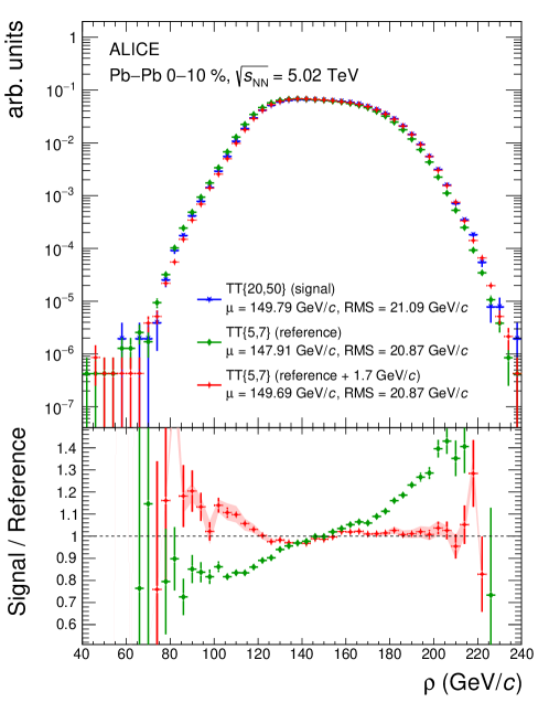
Figure 2: $\rho$ distributions for central Pb–Pb collisions at $\sqrt{s_{\mathrm{NN}}}=5.02$ TeV. Upper panel: $\mathrm{TT}_{\mathrm{sig}}$ and $\mathrm{TT}_{\mathrm{ref}}$ distributions, and the $\mathrm{TT}_{\mathrm{ref}}$ distribution shifted by $\Delta\rho=1.7$ $\mathrm{GeV/}c$ (Sec. 4.1). Lower panel: ratio of $\mathrm{TT}_{\mathrm{ref}}$ and shifted $\mathrm{TT}_{\mathrm{ref}}$ to $\mathrm{TT}_{\mathrm{sig}}$ distribution. The mean ($\mu$) and RMS of the distributions are given in the legend. The vertical lines on the data points are the statistical uncertainties, and the shaded band on the ratio of the $\mathrm{TT}_{\mathrm{sig}}$ over the shifted $\mathrm{TT}_{\mathrm{ref}}$ distributions represents the systematic uncertainty of the procedure.

Figure 2 shows the $\rho$ distributions for the $\mathrm{TT}_{\mathrm{sig}}$ and $\mathrm{TT}_{\mathrm{ref}}$ event selections in this analysis, for central Pb–Pb collisions. While the shapes are similar, the mean of the $\mathrm{TT}_{\mathrm{sig}}$-selected distribution is larger. Shifting the $\mathrm{TT}_{\mathrm{ref}}$-selected distribution to larger values uniformly by $\Delta\rho=1.7$ $\mathrm{GeV/}c$ flattens the ratio of the $\mathrm{TT}_{\mathrm{sig}}$ and $\mathrm{TT}_{\mathrm{ref}}$ distributions with high precision over much of the measured range (Fig. 2, lower panel), and this flatness persists when applying additional shifts in the $\mathrm{TT}_{\mathrm{ref}}$ distribution up to $\pm 0.1$ $\mathrm{GeV/}c$. A shift of $\Delta\rho=1.7\pm{0.1}$ $\mathrm{GeV/}c$ is therefore the optimal $\rho$ calibration for this analysis.

Note that this $\Delta\rho$ calibration procedure was not applied in the ALICE Run 1 analysis of this observable [50], thereby limiting its $p_{\mathrm{T,jet}}$ range and precision.

4.2 Yield calibration: $\mathbf{c_{\mathrm{Ref}}}$

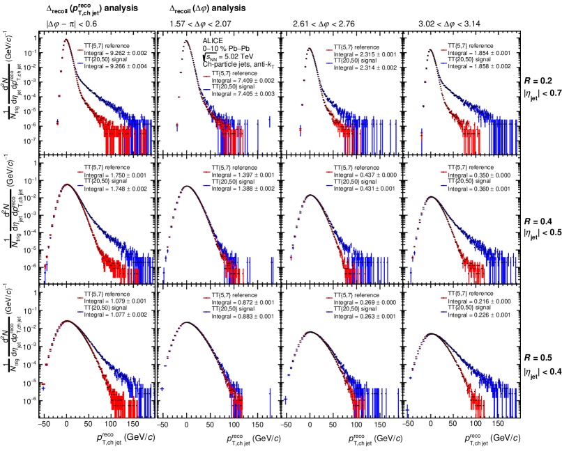
Figure 3: Trigger-normalized semi-inclusive recoil jet distributions for $\mathrm{TT}_{\mathrm{sig}}$ and $\mathrm{TT}_{\mathrm{ref}}$-selected populations in central Pb–Pb collisions at $\sqrt{s_{\mathrm{NN}}}=5.02$ TeV, for $R=0.2$ (upper panels), 0.4 (middle panels), and 0.5 (lower panels). The $\Delta\rho$ correction (Sec. 4.1) has been applied to the $\mathrm{TT}_{\mathrm{ref}}$ distributions. The left column shows distributions in the $\Delta\varphi$ acceptance of the $\Delta_{\mathrm{recoil}}(p_{\mathrm{T,jet}})$ analysis. The remaining columns show distributions in selected $\Delta\varphi$ bins for the $\Delta_{\mathrm{recoil}}(\Delta\varphi)$ analysis, with the second column having the largest deviation from $\Delta\varphi=\pi$ and the rightmost column at $\Delta\varphi\sim\pi$.

Figure 3 shows the trigger-normalized semi-inclusive recoil jet distributions for $\mathrm{TT}_{\mathrm{sig}}$ and $\mathrm{TT}_{\mathrm{ref}}$-selected events in central Pb–Pb collisions for $R=0.2$, 0.4, and 0.5, for a $\Delta\varphi$ interval corresponding to that of the $\Delta_{\mathrm{recoil}}(p_{\mathrm{T,jet}})$ analysis (left panels), and for selected $\Delta\varphi$ bins of the $\Delta_{\mathrm{recoil}}(\Delta\varphi)$ analysis (middle and right panels). The $\mathrm{TT}_{\mathrm{sig}}$ and $\mathrm{TT}_{\mathrm{ref}}$-selected distributions are similar in the region $p_{\mathrm{T,ch~{}jet}}^{\mathrm{reco}}<0$, even though a systematic difference is visible in all panels of Fig. 3. This is consistent with what has been found previously for central A–A collisions in Refs. [50, 70].

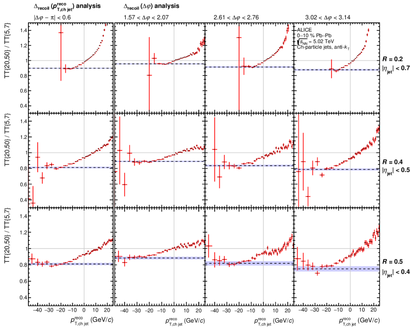
Figure 4: Ratio of $\mathrm{TT}_{\mathrm{sig}}$ and $\mathrm{TT}_{\mathrm{ref}}$-selected distributions from Fig. 3, with the same panel layout. The horizontal dashed line and band show the value of $c_{\mathrm{Ref}}$ and its uncertainty. The vertical solid grey line is at $p_{\mathrm{T,ch~{}jet}}^{\mathrm{reco}}=0$, and horizontal solid grey line is at unity. See text for details.

The integrals of the $\mathrm{TT}_{\mathrm{sig}}$ and $\mathrm{TT}_{\mathrm{ref}}$-selected distributions reported in each panel are consistent to within a few percent, with many of them consistent at the per-mil level (see also Refs. [50, 70]). This invariance, combined with the harder tail of the $\mathrm{TT}_{\mathrm{sig}}$-selected recoil jet distribution at large positive $p_{\mathrm{T,ch~{}jet}}^{\mathrm{reco}}$, implies that the $\mathrm{TT}_{\mathrm{sig}}$ recoil distribution is lower than the $\mathrm{TT}_{\mathrm{ref}}$ recoil distribution in the region $p_{\mathrm{T,ch~{}jet}}^{\mathrm{reco}}<0$. Figure 4 shows the ratio of the $\mathrm{TT}_{\mathrm{sig}}$ and $\mathrm{TT}_{\mathrm{ref}}$-selected distributions for each panel of Fig. 3. The ratio in the negative $p_{\mathrm{T,ch~{}jet}}^{\mathrm{reco}}$ region is indeed less than unity in all cases, as expected.

Notably, for $R=0.4$ and 0.5, the ratio is independent of $p_{\mathrm{T,ch~{}jet}}^{\mathrm{reco}}$ within statistical uncertainties for a significant range in $p_{\mathrm{T,ch~{}jet}}^{\mathrm{reco}}$, i.e. the $\mathrm{TT}_{\mathrm{sig}}$ and $\mathrm{TT}_{\mathrm{ref}}$-selected distributions have the same shape within uncertainties in this region, over which they each vary by several orders of magnitude. For $R=0.2$, this invariance may also be present but cannot be observed clearly in the negative $p_{\mathrm{T,ch~{}jet}}^{\mathrm{reco}}$ region because of the significantly smaller background fluctuations than for larger-$R$ distributions.

Consistency in the shape of the $\mathrm{TT}_{\mathrm{sig}}$ and $\mathrm{TT}_{\mathrm{ref}}$-selected distributions over a significant range in the negative $p_{\mathrm{T,ch~{}jet}}^{\mathrm{reco}}$ region confirms that the yield in this region is dominated by uncorrelated background. To account for the difference in their overall magnitude, the $\mathrm{TT}_{\mathrm{ref}}$ distribution is renormalized by a factor $c_{\mathrm{Ref}}$, as indicated in Eq. 5 [50]. The value of $c_{\mathrm{Ref}}$ is determined for each $\Delta\varphi$ bin using a two-parameter linear fit to the left-most points of the ratio, up to a cutoff value of $p_{\mathrm{T,ch~{}jet}}^{\mathrm{reco}}$. The cutoff value is varied and the slope and its error from the fit are determined. The procedure is terminated at the largest cutoff in $p_{\mathrm{T,ch~{}jet}}^{\mathrm{reco}}$ for which the slope parameter is still consistent with zero within $2\sigma$, indicating the range in $p_{\mathrm{T,ch~{}jet}}^{\mathrm{reco}}$ over which the uncorrelated jet yield dominates both the $\mathrm{TT}_{\mathrm{sig}}$ and $\mathrm{TT}_{\mathrm{ref}}$-selected distributions. The value of $c_{\mathrm{Ref}}$ is then determined by evaluating the fit function in the middle of its range.

Figure 5 shows the trend of $c_{\mathrm{Ref}}$ as a function of $\Delta\varphi$, which is used in the $\Delta_{\mathrm{recoil}}(\Delta\varphi)$ analysis, for $R\ =0.2$, 0.4, and 0.5. The value of $c_{\mathrm{Ref}}$ decreases as $\Delta\varphi$ approaches $\pi$. This is because the largest difference in the $\mathrm{TT}_{\mathrm{sig}}$ and $\mathrm{TT}_{\mathrm{ref}}$ distributions at high $p_{\mathrm{T,ch~{}jet}}^{\mathrm{reco}}$ occurs at $\Delta\varphi=\pi$, where the largest correlated yield is present, resulting in a larger vertical offset between $\mathrm{TT}_{\mathrm{sig}}$ and $\mathrm{TT}_{\mathrm{ref}}$ at $p_{\mathrm{T,ch~{}jet}}^{\mathrm{reco}}<0$. Conversely, the smallest difference occurs at $\Delta\varphi=\pi/2$, where a smaller vertical offset between $\mathrm{TT}_{\mathrm{sig}}$ and $\mathrm{TT}_{\mathrm{ref}}$ at $p_{\mathrm{T,ch~{}jet}}^{\mathrm{reco}}<0$ occurs. The $c_{\mathrm{Ref}}$ values for the $\Delta_{\mathrm{recoil}}(p_{\mathrm{T,jet}})$ analysis are indicated in the figure as horizontal bands.

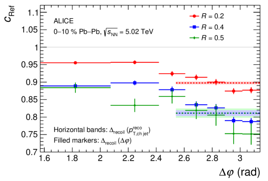
Figure 5: Scaling factor $c_{\mathrm{Ref}}$ of $\Delta_{\mathrm{recoil}}(\Delta\varphi)$ for $R=0.2$, 0.4, and 0.5. The vertical bars indicate the statistical uncertainties. The value of $c_{\mathrm{Ref}}$ for the $\Delta_{\mathrm{recoil}}(p_{\mathrm{T,jet}})$ analysis, which integrates over the region $|\Delta\varphi-\pi|<0.6$, is displayed as a horizontal bar for each value of $R$, with shaded bands indicating statistical uncertainty.

4.3 Qualitative estimate of low-$\mathbf{p_{\mathrm{T,ch\,jet}}}$ kinematic reach

The measurement in central Pb–Pb collisions of recoil jet distributions at low $p_{\mathrm{T,jet}}$, large $R$, and large azimuthal deviation from the back-to-back configuration $\Delta\varphi\sim\pi$ is especially challenging, because of the especially small correlated signal relative to large uncorrelated background. The following sections detail the correction procedures and systematic uncertainties for such measurements. However, it is useful to first look at the raw data for a qualitative assessment of this analysis challenge. Specifically, to what extent can a non-zero correlated signal already be seen in the raw data, in the kinematic region expected to contribute to the low $p_{\mathrm{T,ch~{}jet}}$ region of the fully corrected recoil jet distribution?

Figure 4 can be used to address this question. In each panel, a statistically significant difference between the $\mathrm{TT}_{\mathrm{sig}}$ and $\mathrm{TT}_{\mathrm{ref}}$-selected distributions is evident at negative values of $p_{\mathrm{T,ch~{}jet}}^{\mathrm{reco}}$. However, $p_{\mathrm{T,ch~{}jet}}^{\mathrm{reco}}$ still includes the effect of residual background fluctuations, which are subsequently corrected by unfolding (Sec. 7). The lowest value of $p_{\mathrm{T,ch~{}jet}}^{\mathrm{reco}}$ at which this difference is significant therefore does not indicate directly the low-$p_{\mathrm{T,jet}}$ range achievable in fully-corrected distributions. Nevertheless, that range can be estimated parametrically.

Section 7.2.2 describes the embedding procedure to quantify the magnitude of $p_{\mathrm{T,jet}}$ smearing from residual background fluctuations. The $p_{\mathrm{T,jet}}$-smearing calculated by this procedure is characterized by an RMS of $\sim 6$ $\mathrm{GeV/}c$ for $R=0.2$ and $\sim 17$ $\mathrm{GeV/}c$ for $R=0.5$. In Fig. 4, statistically significant differences between $\mathrm{TT}_{\mathrm{sig}}$ and $\mathrm{TT}_{\mathrm{ref}}$-selected distributions occur in the $p_{\mathrm{T,ch~{}jet}}^{\mathrm{reco}}$ ranges $[-10,-5]$ $\mathrm{GeV/}c$ for $R=0.2$, and $[-20,-15]$ $\mathrm{GeV/}c$ for $R=0.5$. These values of $p_{\mathrm{T,ch~{}jet}}^{\mathrm{reco}}$ are below zero by amounts similar to the RMS values of $p_{\mathrm{T,jet}}$-smearing, and therefore have contributions predominantly from yield in the true recoil jet distribution at very low (positive) values of $p_{\mathrm{T,jet}}$. Based on these considerations of uncorrected data, significant measurements of the corrected recoil jet yield at low $p_{\mathrm{T,ch~{}jet}}$ are expected. Figs. 13 and 14 show that this is indeed achieved by the analysis employing the full correction procedure.

4.4 $\Delta_{\mathrm{recoil}}$ distributions

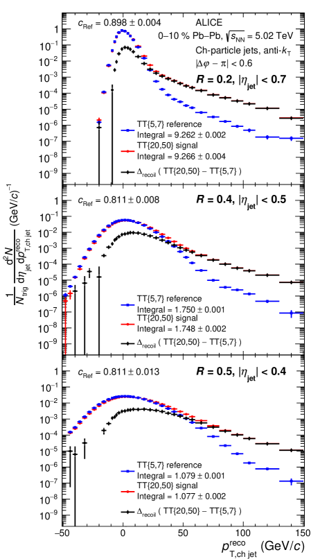
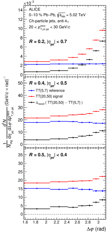
Figure 6: Trigger-normalized semi-inclusive recoil jet distributions for $\mathrm{TT}_{\mathrm{sig}}$ and $\mathrm{TT}_{\mathrm{ref}}$-selected populations in central Pb–Pb collisions at $\sqrt{s_{\mathrm{NN}}}=5.02$ TeV, for $R=0.2$ (top), 0.4 (middle), and 0.5 (bottom). The $\mathrm{TT}_{\mathrm{ref}}$ distribution has the $\Delta\rho$ calibration applied and is scaled by $c_{\mathrm{Ref}}$. The resulting $\Delta_{\mathrm{recoil}}$ distribution is also shown. Left panels: Distributions as a function of $p_{\mathrm{T,ch~{}jet}}^{\mathrm{reco}}$ in the $\Delta\varphi$ acceptance of the $\Delta_{\mathrm{recoil}}(p_{\mathrm{T,jet}})$ analysis. Right panels: Distributions as a function of $\Delta\varphi$, for $p_{\mathrm{T,ch~{}jet}}^{\mathrm{reco}}\in[20,30$] $\mathrm{GeV/}c$. Data points with a negative value for $\Delta_{\mathrm{recoil}}$ are not shown, but all such points are consistent with zero within statistical error.

Figure 6 shows the trigger-normalized recoil distributions for $\mathrm{TT}_{\mathrm{sig}}$ and $\mathrm{TT}_{\mathrm{ref}}$-selected populations in central Pb–Pb collisions for $R=0.2$, 0.4, and 0.5. The $\mathrm{TT}_{\mathrm{ref}}$ distribution is fully calibrated, i.e. the  $\Delta\rho$ correction is applied and its amplitude is scaled by $c_{\mathrm{Ref}}$. The resulting $\Delta_{\mathrm{recoil}}(p_{\mathrm{T,ch~{}jet}}^{\mathrm{reco}})$ (left panels) and $\Delta_{\mathrm{recoil}}(\Delta\varphi)$ (right panels) distributions are shown. The $\Delta_{\mathrm{recoil}}(\Delta\varphi)$ distributions shown correspond to the $20<p_{\mathrm{T,ch~{}jet}}^{\mathrm{reco}}<30$ $\mathrm{GeV/}c$ region. Since $\Delta_{\mathrm{recoil}}$ is the difference between two terms, it can take negative values; however, the vertical axes of the left panels of Fig. 6 use a logarithmic scale and cannot display negative values. Points with negative values for $\Delta_{\mathrm{recoil}}$ are consequently not shown, but in every case are consistent with zero within statistical uncertainties.

Because the $\mathrm{TT}_{\mathrm{sig}}$ and $\mathrm{TT}_{\mathrm{ref}}$-selected distributions at low $p_{\mathrm{T,ch~{}jet}}^{\mathrm{reco}}$ are closely similar in magnitude and vary rapidly, a mismatch in the $p_{\mathrm{T,ch~{}jet}}^{\mathrm{reco}}$ scale of the two distributions would in turn generate a rapidly varying structure in their difference. However, the $\Delta_{\mathrm{recoil}}$ distributions are seen to vary smoothly as a function of $p_{\mathrm{T,ch~{}jet}}^{\mathrm{reco}}$, providing additional validation of the calibration techniques presented above.

5 Measurement of $\Delta_{\mathrm{recoil}}$: pp collisions

In this analysis, medium-induced effects are determined by comparing measurements of Pb–Pb collisions to those of $\mathrm{pp}$ collisions. The observable $\Delta_{\mathrm{recoil}}$ was developed for precise, data-driven correction of the large background accompanying jet measurements in Pb–Pb collisions, which is not present in $\mathrm{pp}$ collisions, and a more conventional approach could suffice for the analysis of $\mathrm{pp}$ data. Nevertheless, for accurate comparison of the two systems, measurements of $\Delta_{\mathrm{recoil}}$ and its projections are likewise reported for $\mathrm{pp}$ collisions. However, since the uncorrelated background is much smaller in $\mathrm{pp}$ than in central Pb–Pb collisions, the calibrations discussed in Sec. 4.1 and 4.2 are simpler. Specifically, the magnitude of $\rho$ is much smaller in $\mathrm{pp}$ collisions, and the $\Delta\rho$ calibration is not required.

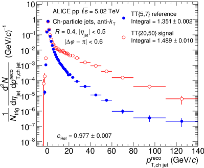
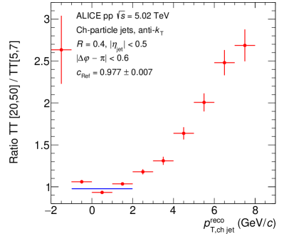
Figure 7: Left: trigger-normalized semi-inclusive recoil jet distributions with $R=0.4$ for $\mathrm{TT}_{\mathrm{sig}}$ and $\mathrm{TT}_{\mathrm{ref}}$-selected populations in $\mathrm{pp}$ collisions at $\sqrt{s}=5.02$ TeV; Right: ratio of the two distributions. The horizontal blue line indicates the fit to the ratio close to $p_{\mathrm{T,ch~{}jet}}^{\mathrm{reco}}=0$ for the determination of $c_{\mathrm{Ref}}$, the value of which is also given in the figures.

Figure 7 shows the uncorrected distribution of semi-inclusive recoil jet distributions for $\mathrm{TT}_{\mathrm{sig}}$ and $\mathrm{TT}_{\mathrm{ref}}$-selected populations in $\mathrm{pp}$ collisions at $\sqrt{s}=5.02$ TeV for $R=0.4$, together with their ratio to determine the value of $c_{\mathrm{Ref}}$. The principal value of $c_{\mathrm{Ref}}$ is determined using a two-parameter linear fit in a narrow range around $p_{\mathrm{T,ch~{}jet}}^{\mathrm{reco}}=0$. The fit range is varied to estimate the systematic uncertainty. The value of $c_{\mathrm{Ref}}$ obtained with this procedure varies between 0.92 and 1.0, depending on $R$. The dependence of $c_{\mathrm{Ref}}$ on $\Delta\varphi$ for the $\Delta_{\mathrm{recoil}}(\Delta\varphi)$ analysis is negligible, and the same value of $c_{\mathrm{Ref}}$ is used for all $\Delta\varphi$ bins for $\mathrm{pp}$ collisions.

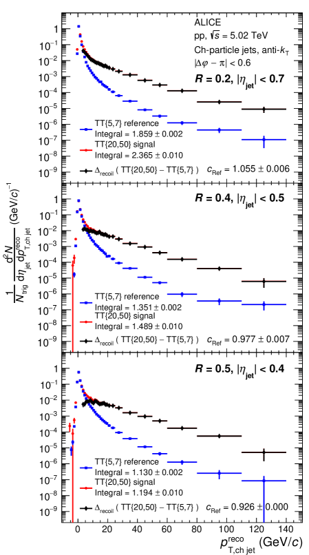
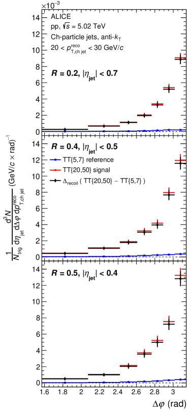
Figure 8: Trigger-normalized semi-inclusive recoil jet distributions for $\mathrm{TT}_{\mathrm{sig}}$ and $\mathrm{TT}_{\mathrm{ref}}$-selected populations in $\mathrm{pp}$ collisions at $\sqrt{s}=5.02$ TeV, for $R=0.2$ (top), 0.4 (middle), and 0.5 (bottom). The $\mathrm{TT}_{\mathrm{ref}}$ distribution is scaled by $c_{\mathrm{Ref}}$. The resulting $\Delta_{\mathrm{recoil}}$ distribution is also shown. Left panels: Distributions as a function of $p_{\mathrm{T,ch~{}jet}}^{\mathrm{reco}}$ in the $\Delta\varphi$ acceptance of the $\Delta_{\mathrm{recoil}}(p_{\mathrm{T,jet}})$ analysis. Right panels: Distributions as a function of $\Delta\varphi$, for $p_{\mathrm{T,ch~{}jet}}^{\mathrm{reco}}\in[20,30$] $\mathrm{GeV/}c$. $\mathrm{TT}_{\mathrm{sig}}$ and $\mathrm{TT}_{\mathrm{ref}}$ distributions in left middle panel are the same as in Fig. 7, left panel.

Figure 8 shows the trigger-normalized recoil distributions for $\mathrm{TT}_{\mathrm{sig}}$ and $\mathrm{TT}_{\mathrm{ref}}$-selected populations, and the corresponding $\Delta_{\mathrm{recoil}}(p_{\mathrm{T,ch~{}jet}}^{\mathrm{reco}})$ and $\Delta_{\mathrm{recoil}}(\Delta\varphi)$ distributions, for $\mathrm{pp}$ collisions at $\sqrt{s}=5.02$ TeV. The distributions correspond to the same $p_{\mathrm{T,ch~{}jet}}^{\mathrm{reco}}$ and $\Delta\varphi$ regions as the Pb–Pb distributions shown in Fig. 6. The $\mathrm{TT}_{\mathrm{ref}}$ component is negligible except in a narrow region around $p_{\mathrm{T,ch~{}jet}}^{\mathrm{reco}}=0$, so that the $\Delta_{\mathrm{recoil}}$ distributions closely match those of the $\mathrm{TT}_{\mathrm{sig}}$-selected population.

6 Theoretical calculations

Monte Carlo (MC) event generators are used both for physics studies and for the simulation of the detector response to correct the measured distributions for instrumental effects.

Simulations used to correct for instrumental effects are carried out with the PYTHIA8 MC generator (Monash 2013 tune) [97, 98]). The detector response is simulated using GEANT 3.21 [99]. In Pb–Pb collisions, additional corrections for the residual background fluctuations are carried out by embedding PYTHIA8 $\mathrm{pp}$ events into Pb–Pb data events, as explained in detail in Sect. 7.

For the simulation of $\mathrm{pp}$ collisions for physics studies, the following MC generators are used:

• PYTHIA8: leading order (LO) pQCD with logarithmic corrections;

• POWHEG [100, 101, 102, 103] with CT14NLO PDFs [104]: calculation of scattering processes via jet pair production [105] up to next-to-leading order (NLO), matched to parton shower and hadronization from PYTHIA8;

• JETSCAPE PP19 tune [106]: based on PYTHIA8, with modified parton shower.

For model calculations in Pb–Pb collisions, the following predictions are used. These models are based on PYTHIA8 (except JEWEL which is based on PYTHIA6 [107]) to generate hard processes, but differ in their treatment of jet–medium interactions and response of the QGP medium to the traversing jet:

• JETSCAPE [108] with Pb–Pb tune [82]: multi-stage, modular MC generator for full simulation of heavy-ion collisions. Partonic evolution in the QGP is modelled using MATTER at high virtuality [109, 110] and LBT at low virtuality [111, 112];

• JEWEL [113, 114]: MC generator which includes both collisional and radiative parton energy loss mechanisms in a pQCD approach. Calculations are carried out in two different ways: (i) including recoiling partons from the medium in the jet finding and subtracting the recoil partons 4-momentum from $p_{\mathrm{T,jet}}$ [81]) (“recoils on, 4MomSub”); and (ii) not including recoiling partons in the jet response (“recoils off”);

• Hybrid Model [35]: MC generator which incorporates both weakly- and strongly-coupled elements of jet quenching by describing the pQCD jet dynamics using DGLAP evolution, and the soft jet-medium interaction using a holographic description based on the AdS/CFT correspondence. Model predictions optionally include the effects of Molière elastic scattering [80] and wake effects.

The acoplanarity distributions are also compared to an analytical calculation:

• pQCD@LO: LO pQCD calculation with Sudakov resummation [76] based on the framework in Refs. [77, 115]. Azimuthal broadening due to gluon radiation in vacuum is treated separately from medium-induced broadening, with the latter controlled by the in-medium jet transport coefficient $\hat{q}$.

7 Corrections

This section presents the corrections for instrumental and background effects. The semi-inclusive distributions reported here have two components: the high-$p_{\mathrm{T}}$ trigger hadron, which is used for event selection, and the reconstructed jets in the selected events. The corrections for each component are discussed in the next subsections.

7.1 Trigger hadrons

As discussed in Ref. [50], high-$p_{\mathrm{T}}$ charged hadrons rather than jets are chosen as the trigger for this analysis because they are measured in central Pb–Pb collisions with high precision event-by-event, without the need for corrections to the complex accompanying background. Tracking efficiency at high-$p_{\mathrm{T}}$ is independent of $p_{\mathrm{T}}$ [116], so that the loss of tracks due to inefficiency is equivalent in this analysis simply to a reduction in integrated luminosity without imposing a bias on the hadron selection. Correction for the trigger hadron tracking efficiency is therefore not required. The effect of track momentum resolution on the selection of trigger hadrons near threshold was found to be negligible in Ref. [50], so is also not considered here.

A potential additional bias is the correlation of the high-$p_{\mathrm{T}}$ hadron distribution with that of the event plane (EP). However, for central Pb–Pb collisions at $\sqrt{s_{\mathrm{NN}}}=2.76$ TeV this bias was found to be negligible [50]. Its magnitude was rechecked for this analysis and again found to be negligible, and this effect is not considered further here.

The azimuthal angle ($\varphi$) resolution of charged tracks is better than $0.5$ $\mathrm{m\,rad}$ for tracks with $p_{\mathrm{T}}>5$ $\mathrm{GeV/}c$, and as such no correction for angular smearing of the trigger track is warranted.

7.2 Reconstructed jet distributions

The measured charged-particle jet distributions are corrected for the effects of both detector response and residual background fluctuations. The detector response corresponds to the effects of tracking inefficiencies, track $p_{\mathrm{T}}$-resolution, and weak-decay background, all of which modify the jet momentum and axis when the jet is reconstructed in both $\mathrm{pp}$ and Pb–Pb collisions. Local fluctuations in the background also smear the reconstructed jet $p_{\mathrm{T}}$ and $\Delta\varphi$ in Pb–Pb collisions.

Corrections for detector response and residual background fluctuations are carried out using an unfolding procedure. For the $\Delta_{\mathrm{recoil}}(p_{\mathrm{T,jet}})$ analysis unfolding is done in one dimension, $p_{\mathrm{T,jet}}$, while for the $\Delta_{\mathrm{recoil}}(\Delta\varphi)$ analysis unfolding is done in two dimensions, $p_{\mathrm{T,jet}}$ and $\Delta\varphi$. ${I}_{\rm AA}(p_{\mathrm{T,ch~{}jet}})$ for the two cases (see Secs. 10.3 and 10.6) are consistent within experimental uncertainties for all $R$, when projected in a common $\Delta\varphi$ acceptance.

7.2.1 Parameterized detector performance

While the unfolding procedure is carried out using the full response matrices described below, key parameters that characterize the detector performance for jet reconstruction are summarized here for reference. These quantities are not used for correction of the data.

$\mathbf{p_{\mathrm{T,jet}}}$ resolution and median $\mathbf{p_{\mathrm{T,jet}}}$ shift:

The detector effects which smear the $p_{\mathrm{T,jet}}$ distribution are characterized in $\mathrm{pp}$ simulations with the relative difference between the $p_{\mathrm{T,jet}}$ at detector level and particle level, $(p_{\mathrm{T,ch~{}jet}}^{\mathrm{det}}-p_{\mathrm{T,ch~{}jet}}^{\mathrm{part}})/p_{\mathrm{T,ch~{}jet}}^{\mathrm{part}}$  [117]. Table  1 shows the width and median shift of this distribution for $R=0.2$ and 0.5 in selected $p_{\mathrm{T,ch~{}jet}}^{\mathrm{part}}$ intervals. Since a value of $p_{\mathrm{T,ch~{}jet}}^{\mathrm{det}}$ larger than $p_{\mathrm{T,ch~{}jet}}^{\mathrm{part}}$ can only arise from $p_{\mathrm{T,jet}}$ resolution effects, and the distribution is not symmetric about zero, the $p_{\mathrm{T,jet}}$ resolution is determined by fitting a Gaussian function to the distribution for $(p_{\mathrm{T,ch~{}jet}}^{\mathrm{det}}-p_{\mathrm{T,ch~{}jet}}^{\mathrm{part}})/p_{\mathrm{T,ch~{}jet}}^{\mathrm{part}}>0$ while fixing the mean of the fit to zero, since resolution effects are symmetric. The median relative $p_{\mathrm{T,ch~{}jet}}^{\mathrm{part}}$ shift, which is non-zero due to detector inefficiencies, is also reported. These values are representative of the instrumental effects in both $\mathrm{pp}$ and Pb–Pb collisions.

Table 1: The resolution and median of the relative smearing of $p_{\mathrm{T,jet}}$ due to detector effects, $S=(p_{\mathrm{T,ch~{}jet}}^{\mathrm{det}}-p_{\mathrm{T,ch~{}jet}}^{\mathrm{part}})/p_{\mathrm{T,ch~{}jet}}^{\mathrm{part}}$, for $R=0.2$ and 0.5 in selected $p_{\mathrm{T,ch~{}jet}}^{\mathrm{part}}$ intervals. Values are expressed in percentages.

	$R=0.2$			$R=0.5$
$p_{\mathrm{T,ch~{}jet}}^{\mathrm{part}}$[$\mathrm{GeV/}c$]	$\sigma^{\mathrm{RHS}}(S$)	$\mathrm{median}(S)$		$\sigma^{\mathrm{RHS}}(S$)	$\mathrm{median}(S)$
$[5,10]$	0.9%	$-$0.3%		0.7%	$-$3%
$[50,100]$	1.8%	$-$9%		1.7%	$-$10%

$\Delta\varphi$ resolution:

The resolution in $\Delta\varphi$, denoted $\sigma_{\Delta\varphi}$, is the standard deviation of the difference between the detector-level and truth-level jet values of $\Delta\varphi$. Table 2 shows $\sigma_{\Delta\varphi}$ for $R=0.2$ and $R=0.5$ jets for selected $p_{\mathrm{T,jet}}$ intervals in simulations of Pb–Pb and $\mathrm{pp}$ collisions. The resolution is due to detector effects in $\mathrm{pp}$ collisions, and to both detector effects and background fluctuations in Pb–Pb collisions. The resolution is finer for high $p_{\mathrm{T,ch~{}jet}}^{\mathrm{part}}$ and small $R$. Note that $\sigma_{\Delta\varphi}$ is smaller than the width of the $\Delta\varphi$ bins in the analysis, and therefore corresponds to only a small correction in $\Delta\varphi$.

Table 2: Azimuthal difference resolution $\sigma_{\Delta\varphi}$ for $R=0.2$ and 0.5 in $\mathrm{pp}$ and Pb–Pb collisions in selected $p_{\mathrm{T,ch~{}jet}}^{\mathrm{part}}$ intervals. Values are expressed in radians.

	$R=0.2$			$R=0.5$
$p_{\mathrm{T,ch~{}jet}}^{\mathrm{part}}$[$\mathrm{GeV/}c$]	$\sigma_{\Delta\varphi}$ (Pb–Pb)	$\sigma_{\Delta\varphi}$ ($\mathrm{pp}$)		$\sigma_{\Delta\varphi}$ (Pb–Pb)	$\sigma_{\Delta\varphi}$ ($\mathrm{pp}$)
$[10,20]$	0.05	0.020		0.13	0.05
$[50,100]$	0.013	0.015		0.09	0.03

7.2.2 Unfolding

In the $\mathrm{pp}$ analysis, the response matrix for unfolding is constructed using $\mathrm{pp}$ events simulated using the PYTHIA8 [97] event generator and the GEANT3 [99] transport code. Detector-level jets are matched to particle-level jets based on their relative separation in rapidity and azimuth, $\Delta R=\sqrt{\Delta\eta^{2}+\Delta\varphi^{2}}$, and requiring $\Delta R$ to be less than 0.15 for $R=0.2$ jets, 0.25 for $R=0.4$ jets, and 0.35 for $R=0.5$.

For Pb–Pb collisions, the response matrix accounts for both background fluctuations and detector response. It is constructed by embedding detector-level $\mathrm{pp}$ events simulated with PYTHIA8 into real Pb–Pb data, and matching the PYTHIA8 detector-level jets with jets reconstructed from the combined event. The matching procedure requires the PYTHIA8 detector-level jet to share constituents carrying at least $50\%$ of its total $p_{\mathrm{T}}$ with the PYTHIA8+Pb–Pb detector-level jet.

Unfolding is carried out using the iterative Bayesian algorithm implemented in the RooUnfold package [118]. For the $\Delta_{\mathrm{recoil}}(p_{\mathrm{T,jet}})$ analysis, unfolding is carried out in one dimension to correct $p_{\mathrm{T,ch~{}jet}}^{\mathrm{reco}}$, taking advantage of the fact that the $\Delta\varphi$ resolution correction is small. For the $\Delta_{\mathrm{recoil}}(\Delta\varphi)$ analysis, two-dimensional unfolding is used to correct both $p_{\mathrm{T,ch~{}jet}}^{\mathrm{reco}}$ and $\Delta\varphi$. Crucial to this analysis is the ability to include the full $p_{\mathrm{T,ch~{}jet}}^{\mathrm{reco}}$ range in the unfolding, which is enabled by the subtraction of the entire combinatorial background yield; the full $\Delta_{\mathrm{recoil}}$ range shown in Figs. 6 and 8 is therefore used in the unfolding.

The regularization parameter, which for iterative Bayesian unfolding is the number of iterations, is optimized using both a consistency test between the raw and back-folded distributions, and the requirement that unfolded distributions from successive iterations have minimal variation. The optimal regularization parameters lie between 4 and 8, depending on collision system and jet $R$.

A key element of the unfolding procedure is the choice of prior. For the Pb–Pb analysis the prior is based on the $\Delta_{\mathrm{recoil}}$ distribution calculated with JEWEL (recoils off), and for the $\mathrm{pp}$ analysis the prior is based on the $\Delta_{\mathrm{recoil}}$ distribution calculated with PYTHIA8. The distributions are fitted with a smooth function to remove the effect of finite statistical precision in the MC generation.

For the one-dimensional $\Delta_{\mathrm{recoil}}(p_{\mathrm{T,jet}})$ analysis, the prior $\Delta_{\mathrm{recoil}}(p_{\mathrm{T,jet}})$ distribution is fitted with an exponential function $\Delta(p_{\mathrm{T,jet}})=p_{1}\exp(-p_{2}\times p_{\mathrm{T,jet}}+p_{3}\times(p_{\mathrm{T,jet}})^{p_{4}})$, where $p_{1,2,3,4}$ are fit parameters. In the $\mathrm{pp}$ analysis, this function is used as the prior, $P(p_{\mathrm{T,jet}})$. In the Pb–Pb analysis, at low $p_{\mathrm{T,jet}}$ the prior is less constrained in models and significant discrepancies between the prior and unfolded solution can lead to unstable unfolding. For this reason, additional regulation to $P(p_{\mathrm{T,jet}})$ is required. The prior in the Pb–Pb analysis is therefore defined as $P(p_{\mathrm{T,jet}})=K\times(1-f(p_{\mathrm{T,jet}}))+\Delta(p_{\mathrm{T,jet}})\times f(p_{\mathrm{T,jet}})$, where $K$ is a constant defining the magnitude of the prior at low $p_{\mathrm{T,jet}}$ and $f(p_{\mathrm{T,jet}})$ is a cutoff function, $f(p_{\mathrm{T,jet}})=0.5\times(\tanh{[(p_{\mathrm{T,jet}}-a)/b]}+1)$, where $a$ and $b$ are constants. This function allows the prior to tend towards $K$ for $p_{\mathrm{T,jet}}<a$ and towards $\Delta_{\mathrm{recoil}}$(JEWEL) for $p_{\mathrm{T,jet}}>a$. This definition takes into account that jets with radius $R$ subtend finite area and their total number in the acceptance is limited in practice. The three constants are defined separately for each jet $R$ analysis, based on an iterative procedure in which each constant is varied independently, and the values that provide good convergence of unfolding are chosen.

For the $\Delta_{\mathrm{recoil}}(\Delta\varphi)$ $\mathrm{pp}$ and Pb–Pb analyses, the $\Delta\varphi$ projections of the prior are parameterized with a function defined as $g(\Delta\varphi)=q_{1}\times\exp(\frac{\Delta\varphi-\pi}{\sigma})+q_{2}$, where $q_{1,2}$ and $\sigma$ are fit parameters. The function $g(\Delta\varphi)$ is used to fit the $\Delta\varphi$ distribution for each $p_{\mathrm{T,jet}}$ bin separately. The function $g(\Delta\varphi)$ in each $p_{\mathrm{T,jet}}$ interval is then scaled such that the integral of $g(\Delta\varphi)$ in the region $|\Delta\varphi-\pi|<0.6$ is equal to $P(p_{\mathrm{T,jet}})$ in the same $p_{\mathrm{T,jet}}$ region.

The unfolding procedure is validated through a full closure test in simulation, detailed in Sec. 9.

7.2.3 Jet-finding efficiency

An efficiency correction, which is a function of $p_{\mathrm{T,ch~{}jet}}$ and $\Delta\varphi$, is applied to the unfolded spectrum to account for the loss of jets outside the measured range due to smearing effects. In Pb–Pb collisions, this efficiency is calculated using PYTHIA8-generated $\mathrm{pp}$ events embedded into Pb–Pb data. For the $\Delta_{\mathrm{recoil}}(p_{\mathrm{T,jet}})$ analysis, for $R=0.2$ the efficiency is greater than 99% over the full $p_{\mathrm{T,ch~{}jet}}$ range, while for $R=0.5$ the efficiency is around 92% at $p_{\mathrm{T,ch~{}jet}}=10$ $\mathrm{GeV/}c$, rising to unity at $p_{\mathrm{T,ch~{}jet}}=100$ $\mathrm{GeV/}c$ and dropping to 96% at $p_{\mathrm{T,ch~{}jet}}=130$ $\mathrm{GeV/}c$. For the $\Delta_{\mathrm{recoil}}(\Delta\varphi)$ analysis, this efficiency is around 93% for $R=0.2$ and above 70% for $R=0.5$ in the region $\Delta\varphi\sim\pi/2$, increasing as $\Delta\varphi$ approaches $\pi$. In $\mathrm{pp}$ collisions, the efficiency is calculated using PYTHIA8 simulations. For the $\Delta_{\mathrm{recoil}}(p_{\mathrm{T,jet}})$ analysis, the efficiency for all $R$ is greater than 97% for $p_{\mathrm{T,ch~{}jet}}=10$ $\mathrm{GeV/}c$, and consistent with unity at $p_{\mathrm{T,ch~{}jet}}=140$ $\mathrm{GeV/}c$. For the $\Delta_{\mathrm{recoil}}(\Delta\varphi)$ analysis, the efficiency is about 97% for $R=0.2$ (95% for $R=0.5$) at $\Delta\varphi\sim\pi/2$, increasing to 99% for $R=0.2$ (96% for $R=0.5$) at $\Delta\varphi\sim\pi$.

An additional efficiency correction is applied after unfolding to account for the probability of reconstructing a particle-level jet, i.e. for the matching efficiency when constructing the response matrix. This factor is calculated using PYTHIA8 simulations of $\mathrm{pp}$ events, as the ratio of detector-level and particle-level jet yield. It is found to be independent of $\Delta\varphi$. In Pb–Pb collisions, this efficiency is around 90% at $p_{\mathrm{T,ch~{}jet}}=10$ $\mathrm{GeV/}c$ and around 98% at $p_{\mathrm{T,ch~{}jet}}=100$ $\mathrm{GeV/}c$. In pp collisions, it is approximately 92% at $p_{\mathrm{T,ch~{}jet}}=10$ $\mathrm{GeV/}c$ and 100% at $p_{\mathrm{T,ch~{}jet}}=100$ $\mathrm{GeV/}c$.

8 Systematic Uncertainties

For the $\mathrm{pp}$ and Pb–Pb analyses, the systematic uncertainties are due to the tracking-efficiency uncertainty, the uncertainty on the scaling factor $c_{\mathrm{Ref}}$, and the unfolding uncertainties, which include uncertainties due to the choice of prior, the choice of regularization parameter, the $p_{\mathrm{T,jet}}$ binning choice, and the unfolding method. For the Pb–Pb analysis, additional sources include the uncertainty due to the $\Delta\rho$ correction, the jet matching, and the unfolding non-closure. Tables 3 and 4 present a summary of the systematic uncertainties in $\mathrm{pp}$ and Pb–Pb collisions, respectively.

Table 3: Relative systematic uncertainties (in %) for the analysis of $\mathrm{pp}$ collision data for $\Delta_{\mathrm{recoil}}(p_{\mathrm{T,jet}})$ and $\Delta_{\mathrm{recoil}}(\Delta\varphi)$ at $\Delta\varphi=\pi$ and $\pi/2$. Uncertainties are given for the lowest and highest measured values of $p_{\mathrm{T,ch~{}jet}}$. Where the uncertainty is less than 0.1%, it is specified as ‘negl.’ in the table. Where the uncertainty is not applicable, it is specified as ‘X’.

	$\Delta_{\mathrm{recoil}}(p_{\mathrm{T,jet}})$			$\Delta_{\mathrm{recoil}}(\Delta\varphi)$; $\Delta\varphi\sim\pi/2$			$\Delta_{\mathrm{recoil}}(\Delta\varphi)$; $\Delta\varphi\sim\pi$
$R=0.2$	[7, 10] $\mathrm{GeV/}c$xx	[110, 140] xx		[10, 20] xx	[50, 100] xx		[10, 20] xx	[50, 100] xx
Tracking efficiency	0.2%	8.6		14.5	7.9		4.1	17.2
$c_{\mathrm{Ref}}$	1.0	negl.		0.8	0.5		0.4	negl.
Prior	8.1	7.5		negl.	0.5		negl.	0.3
Regularization parameter	0.3	1.0		0.3	4.4		0.1	0.3
Binning	1.0	0.2		negl.	3.3		1.9	0.9
Unfolding method	0.6	6.0		X	X		X	X
Total uncertainty	8.2	12.3		14.6	9.7		4.6	17.3
$R=0.4$	[7, 10] $\mathrm{GeV/}c$xx	[110, 140] xx		[10, 20] xx	[50, 100] xx		[10, 20] xx	[50, 100] xx
Tracking efficiency	3.5%	10.0		11.9	10.9		3.7	14.0
$c_{\mathrm{Ref}}$	0.1	negl.		0.2	0.2		0.2	negl.
Prior	5.9	15.9		negl.	1.7		0.1	0.9
Regularization parameter	2.4	4.8		0.2	5.4		0.8	0.6
Binning	1.7	1.8		0.9	0.9		1.4	0.5
Unfolding method	6.0	6.0		X	X		X	X
Total uncertainty	9.5	20.4		11.9	12.3		4.1	14.1
$R=0.5$	[7, 10] $\mathrm{GeV/}c$xx	[110, 140] xx		[10, 20] xx	[50, 100] xx		[10, 20] xx	[50, 100] xx
Tracking efficiency	3.3%	10.0		8.2	18.1		8.6	7.5
$c_{\mathrm{Ref}}$	0.4	negl		1.4	negl.		1.8	0.2
Prior	6.9	13.6		0.1	0.9		negl.	1.0
Regularization parameter	12.5	6.4		1.0	3.0		0.3	0.9
Binning	0.7	0.8		0.6	0.8		3.7	0.2
Unfolding method	4.4	5.9		X	X		X	X
Total uncertainty	15.3	19.0		8.4	18.4		9.5	7.6

Table 4: Same as Table 3, for Pb–Pb collisions. Where the uncertainty is less than 0.1%, it is specified as ‘negl.’ in the table. Where the uncertainty is not applicable, it is specified as ‘X’.

	$\Delta_{\mathrm{recoil}}(p_{\mathrm{T,jet}})$			$\Delta_{\mathrm{recoil}}(\Delta\varphi)$;$\Delta\varphi\sim\pi/2$			$\Delta_{\mathrm{recoil}}(\Delta\varphi)$;$\Delta\varphi\sim\pi$
$R=0.2$	[7, 10] $\mathrm{GeV/}c$xx	[110, 140] xx		[10, 20] xx	[50, 100] xx		[10, 20] xx	[50, 100] xx
Tracking efficiency	1.3%	6.7		4.1	7.8		3.3	5.5
$c_{\mathrm{Ref}}$	1.7	negl.		3.5	1.3		2.2	0.4
Prior	36.2	0.3		28.1	6.4		29.6	1.7
Regularization parameter	0.8	4.2		3.2.	3.6		7.3	5.0
Binning	10.3	negl.		5.6	5.1		4.7	1.4
Unfolding method	6.5	16.0		X	X		X	X
Jet matching	10.1	0.6		11.9	0.7		4.2	0.6
$\Delta\rho$	1.5	negl.		2.8	2.5		0.4	0.3
Closure	X	X		X	X		X	X
Total uncertainty	39.6	17.9		31.8	12.2		31.4	7.8
$R=0.4$	[7, 10] $\mathrm{GeV/}c$xx	[110, 140] xx		[10, 20] xx	[50, 100] xx		[10, 20] xx	[50, 100] xx
Tracking efficiency	1.0%	7.2		2.1	10.5		0.8	5.1
$c_{\mathrm{Ref}}$	0.1	negl.		2.8	1.5		5.4	1.4
Prior	5.4	2.7		14.1	54.4		5.8	9.7
Regularization parameter	0.6	1.3		2.5	12.9		1.0	5.0
Binning	9.7	0.8		8.4	6.9		6.2	1.8
Unfolding method	4.4	13.8		X	X		X	X
Jet matching	1.0	0.7		6.6	0.2		4.2	3.9
$\Delta\rho$	5.8	0.4		8.1	3.8		3.4	0.9
Closure	22.6	X		X	X		X	X
Total uncertainty	26.3	16.0		19.9	57.4		11.5	12.9
$R=0.5$	[7, 10] $\mathrm{GeV/}c$xx	[110, 140] xx		[10, 20] xx	[50, 100] xx		[10, 20] xx	[50, 100] xx
Tracking efficiency	9.1%	9.2		14.9	8.8		1.0	3.5
$c_{\mathrm{Ref}}$	5.8	0.4		11.1	19.7		11.2	5.8
Prior	11.3	12.6		19.6	19.1		7.2	4.1
Regularization parameter	1.2	8.6		2.8	21.8		1.6	2.1
Binning	5.9	0.4		5.4	7.8		4.0	1.6
Unfolding method	5.6	11.7		X	X		X	X
Jet matching	2.0	0.9		2.9	2.3		0.3	5.3
$\Delta\rho$	11.9	0.5		10.5	3.1		6.2	2.2
Closure	20.5	X		X	X		X	X
Total uncertainty	29.6	21.3		29.7	37.1		15.4	10.1

The tracking-efficiency uncertainty is estimated by modifying the response matrix used in the unfolding procedure via random rejection of a given fraction of tracks prior to jet finding, with the fraction corresponding to the uncertainty of the single-track efficiency. The single-track efficiency and its corresponding uncertainty is the combination of two contributions. The first contribution originates from the track selection criteria in the TPC. The second contribution originates from the matching of TPC tracks to the ITS hits. In $\mathrm{pp}$ collisions, the single-track efficiency uncertainty is approximately 3%, while in central Pb–Pb collisions, its value is approximately 6% for tracks with $p_{\mathrm{T}}=1$ $\mathrm{GeV/}c$, decreasing to approximately 3% for tracks with $p_{\mathrm{T}}=15$ $\mathrm{GeV/}c$ and above. The systematic uncertainty is the relative change in the unfolded result obtained with the modified response matrix with respect to the principal analysis.

The uncertainty in $c_{\mathrm{Ref}}$ in Pb–Pb collisions is estimated by varying the minimum and maximum values of $p_{\mathrm{T,ch~{}jet}}^{\mathrm{reco}}$ used in the fit of the ratios in Fig. 4, as well as the $p_{\mathrm{T,ch~{}jet}}^{\mathrm{reco}}$ value used to determine $c_{\mathrm{Ref}}$. The fit range is varied by $\pm 2$ $\mathrm{GeV/}c$ for $R=0.2$, $\pm 3$ $\mathrm{GeV/}c$ for $R=0.4$, and $\pm 4$ $\mathrm{GeV/}c$ for $R=0.5$, with the larger range for larger $R$ accounting for the wider $c_{\mathrm{Ref}}$ fit range. For $\mathrm{pp}$ collisions, the uncorrelated background is smaller and the fit range to extract $c_{\mathrm{Ref}}$ is narrower. The $c_{\mathrm{Ref}}$ uncertainty is evaluated by varying the range of $\Delta\varphi$ in the vicinity of $p_{\mathrm{T}}=0$. In both $\mathrm{pp}$ and Pb–Pb collisions, the uncertainty reduces as $p_{\mathrm{T,ch~{}jet}}^{\mathrm{reco}}$ increases due to the fact that the subtraction of the $\mathrm{TT}_{\mathrm{ref}}$-selected distribution is a smaller relative correction at large $p_{\mathrm{T,ch~{}jet}}^{\mathrm{reco}}$.

The uncertainties due to the unfolding are assessed by varying its configuration. For $\mathrm{pp}$ collisions, the systematic uncertainty due to the prior utilized in the unfolding is determined by varying the value of the power in the functional form used to fit the prior. For Pb–Pb collisions, the prior knowledge of the yield at low $p_{\mathrm{T,ch~{}jet}}$ is not well constrained, and thus the largest uncertainty in the prior arises from the shape of the low-$p_{\mathrm{T,ch~{}jet}}$ distribution within the function used fit it (see Sec. 7.2.2). The uncertainty on the prior is therefore assessed by varying the value of the parameters $a$ and $K$, while also requiring convergent unfolding without a substantial increase in the required number of iterations with respect to the principle analysis. For both collision systems, the unfolding algorithm uncertainty is assessed by utilizing SVD [119] as an alternative algorithm (where possible when performing 1-dimensional unfolding), and by varying the regularization parameter in the iterative Bayesian unfolding by $\pm 2$. The uncertainty related to the binning choice was assessed by varying the detector-level $p_{\mathrm{T,jet}}$ binning, and by varying the minimum and maximum particle-level $p_{\mathrm{T,jet}}$ bin limits. For the Pb–Pb analysis, there is an additional source of systematic uncertainty related to the jet matching criteria when matching the PYTHIA8 detector-level jets with the PYTHIA8+Pb–Pb detector-level jets. This is estimated by varying the matching distance between the PYTHIA8 and PYTHIA8+Pb–Pb detector-level jets between $0.5R$ and $0.6R$.

In Pb–Pb collisions, the $\rho$ correction parameter $\Delta\rho$ (introduced in Sec. 4.1) is determined based on a fit to the ratio of the $\rho$ distributions for $\mathrm{TT}_{\mathrm{sig}}$ and $\mathrm{TT}_{\mathrm{ref}}$-selected data. However, there remain residual differences between the two distributions. The systematic uncertainty due to $\Delta\rho$ is determined by varying the shift by $\pm 0.1$ $\mathrm{GeV/}c$.

The closure test for the $\Delta_{\mathrm{recoil}}(p_{\mathrm{T,jet}})$ analysis in Pb–Pb collisions also demonstrates moderate non-closure at low $p_{\mathrm{T,jet}}$ (see Sec. 9 for details). In the regions where the closure discrepancy is not covered by the systematic uncertainties listed above, the relative discrepancy is considered as an additional systematic uncertainty. For the $\Delta_{\mathrm{recoil}}(p_{\mathrm{T,jet}})$ and $\Delta_{\mathrm{recoil}}(\Delta\varphi)$ analyses in $\mathrm{pp}$ collisions the unfolding closure is successful for all $p_{\mathrm{T,jet}}$ and $\Delta\varphi$, so no uncertainty is assigned.

In $\mathrm{pp}$ collisions, the effect of the underlying event subtraction is checked by performing the analysis with and without underlying event subtraction. For $p_{\mathrm{T,ch~{}jet}}^{\mathrm{reco}}>5$ $\mathrm{GeV/}c$, the $\Delta_{\mathrm{recoil}}$ distributions with and without this subtraction are fully consistent within the statistical uncertainties, and no uncertainty is therefore assigned.

The total uncertainty is the quadrature sum of the systematic uncertainties from each distinct source. For the yield ratios ${I}_{\rm AA}(p_{\mathrm{T,ch~{}jet}})$ (presented in Sec. 10.3) and ${I}_{\rm AA}(\Delta\varphi)$ (discussed in Sec. 10.6), the systematic uncertainties in the Pb–Pb and $\mathrm{pp}$ measurements are assumed to be uncorrelated, and the uncertainty of ${I}_{\rm AA}(p_{\mathrm{T,ch~{}jet}})$ is computed as their quadrature sum.

9 Closure test

A closure test is carried out on the Pb–Pb analysis to validate the full correction procedure and systematic uncertainties presented in Secs. 7 and 8. The closure test utilizes hybrid events, in which detector-level $\mathrm{pp}$ collisions generated by PYTHIA8 are embedded into real Pb–Pb data events. The raw pseudo-data distributions from the hybrid events are then modified bin-by-bin to introduce the statistical precision of the real data, by adding jitter to the central value using a Gaussian-distributed random function whose $\sigma$ is the statistical uncertainty of data in the bin.

A full analysis is carried out on these events, with the trigger track required to originate from the PYTHIA8 $\mathrm{pp}$ event. Recoil jets are reconstructed, and the $\rho$ correction and $\Delta\rho$ calibration are applied using tracks from the full hybrid event. The raw distributions are then unfolded, the efficiency corrections are applied, and the systematic uncertainties are determined as in the analysis of real data. However, the systematic uncertainty due to the tracking efficiency is not included, since the tracking efficiency entering the raw-level distribution and the response matrix are both from the PYTHIA8 simulation, and therefore are consistent by definition.

This smearing procedure is carried out 20 times. The mean value of the resulting distribution of unfolded solutions is assigned as the central value of the unfolded result, and the RMS of the unfolded solutions is assigned as the statistical uncertainty. The quality of the closure is then judged by comparing the fully-corrected $\Delta_{\mathrm{recoil}}$ distributions with the particle-level $\Delta_{\mathrm{recoil}}$ distribution used as input.

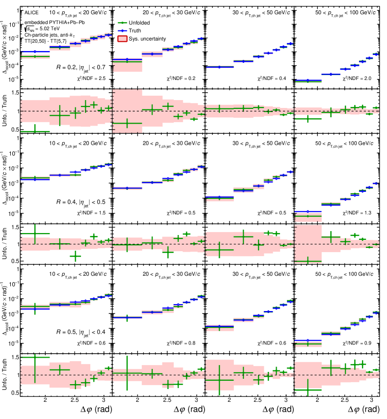
Figure 9: Closure test of $\Delta_{\mathrm{recoil}}(\Delta\varphi)$ analysis for central Pb–Pb collisions, for $R=0.2$, 0.4, and 0.5 in selected $p_{\mathrm{T,ch~{}jet}}$ bins.

Figure 9 shows the result of the closure test for the $\Delta_{\mathrm{recoil}}(\Delta\varphi)$ analysis of central Pb–Pb collisions, comparing the unfolded result with the PYTHIA8-generated particle-level distribution. Each panel shows $\chi^{2}$/NDF from the comparison of the unfolded and particle-level distributions. While moderate discrepancies occur in the tail of the $\Delta\varphi$ distribution, farthest from $\Delta\varphi\sim\pi$, the distributions are in agreement within uncertainties, indicating successful closure.

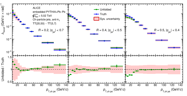
Figure 10: Closure test of $\Delta_{\mathrm{recoil}}(p_{\mathrm{T,jet}})$ analysis for central Pb–Pb collisions.

Figure 10 shows the result of the closure test for the $\Delta_{\mathrm{recoil}}(p_{\mathrm{T,jet}})$ analysis of central Pb–Pb collisions. Good closure is likewise achieved over most of the $p_{\mathrm{T,jet}}$ range. However, for $R=0.5$ and $R=0.4$ at low-$p_{\mathrm{T,jet}}$, the distribution falls outside of the uncertainty of the unfolded result; in this case the relative magnitude of the discrepancy is included as a source of systematic uncertainty, as reported in Tab. 4.

10 Results

This section presents corrected $\Delta_{\mathrm{recoil}}(p_{\mathrm{T,ch~{}jet}},\Delta\varphi)$ distributions for $\mathrm{pp}$ and central Pb–Pb collisions and physics results from their comparison. Key results are presented in the companion Letter [75].

10.1 $\Delta_{\mathrm{recoil}}(p_{\mathrm{T,ch~{}jet}})$ in pp collisions

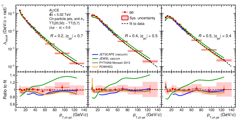
Figure 11: Upper panels: corrected $\Delta_{\mathrm{recoil}}(p_{\mathrm{T,ch~{}jet}})$ distributions measured for $R=0.2$ (left), 0.4 (middle), and 0.5 (right) in $\mathrm{pp}$ collisions at $\sqrt{s}=5.02$ TeV, compared to calculations from JETSCAPE  [108], JEWEL  [113, 114], PYTHIA8  [97, 98], and POWHEG  [100, 101, 102, 103]. Lower panels: ratio of the data and calculations to a functional fit of the measured $\Delta_{\mathrm{recoil}}(p_{\mathrm{T,ch~{}jet}})$ distributions.

Figure 11, upper panels, show fully-corrected $\Delta_{\mathrm{recoil}}(p_{\mathrm{T,ch~{}jet}})$ distributions for $R=0.2,~{}0.4$, and 0.5 measured in $\mathrm{pp}$ collisions at $\sqrt{s}=5.02$ TeV, together with comparison to model calculations based on PYTHIA8 Monash 2013 tune [97, 98], JEWEL (vacuum) [120, 114], JETSCAPE (vacuum) [106], and POWHEG [105]. Figure 11, lower panels, show the ratio of the distributions in the upper panels to the fit of a smooth function to the data, in order to suppress fluctuations in the data for comparison purposes. The same smoothing procedure is used in the lower panels of Figs. 12, 13, and 14.

The PYTHIA8 and JETSCAPE calculations agree with the data within experimental uncertainties over the full $p_{\mathrm{T,ch~{}jet}}$ range. These calculations are related, since JETSCAPE utilizes PYTHIA8 for hard process generation and string fragmentation, with independent procedures for final-state parton showering and hadronization. These independent processes are expected to have little effect on jet distributions, however. The POWHEG calculations likewise describe the data well over the full $p_{\mathrm{T,ch~{}jet}}$ range. The JEWEL calculation does not describe $p_{\mathrm{T,ch~{}jet}}$-dependence of $\Delta_{\mathrm{recoil}}(p_{\mathrm{T,ch~{}jet}})$ well, overestimating the data for $p_{\mathrm{T,ch~{}jet}}$ $>30$ $\mathrm{GeV/}c$, with $\sim$40% disagreement at high $p_{\mathrm{T,ch~{}jet}}$.

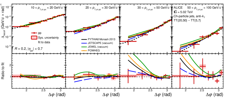
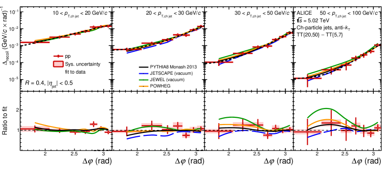
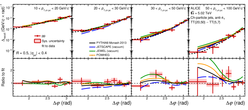
Figure 12: Corrected $\Delta_{\mathrm{recoil}}(\Delta\varphi)$ distributions for $\mathrm{pp}$ collisions at $\sqrt{s}=5.02$ TeV for $R=0.2$ (top), 0.4 (middle), and 0.5 (bottom) in $p_{\mathrm{T,ch~{}jet}}$ bins (left to right): [10,20], [20,30], [30,50], and [50,100] $\mathrm{GeV/}c$. JETSCAPE, JEWEL, PYTHIA8, and POWHEG calculations are also shown. Upper sub-panels show the individual distributions, while lower sub-panels show their ratio to a functional fit of the measured data.

Figure 12 shows corrected $\Delta_{\mathrm{recoil}}(\Delta\varphi)$ distributions for $R=0.2$, 0.4, and 0.5 measured in $\mathrm{pp}$ collisions at $\sqrt{s}=5.02$ TeV in various $p_{\mathrm{T,ch~{}jet}}$ bins, together with comparisons to theoretical calculations. The JETSCAPE calculation agrees with the data within uncertainties in all panels. The other calculations also agree with the data within uncertainties except for $\Delta\varphi\lesssim 2.5$ in the ranges $p_{\mathrm{T,ch~{}jet}}>30$ $\mathrm{GeV/}c$ for $R=0.2$ (PYTHIA8, POWHEG, JEWEL), and $p_{\mathrm{T,ch~{}jet}}>50$ $\mathrm{GeV/}c$ for $R=0.5$ (POWHEG, JEWEL). These $\mathrm{pp}$ data provide the reference for comparison to same distributions measured in Pb–Pb collisions, to explore medium-induced effects.

10.2 $\Delta_{\mathrm{recoil}}(p_{\mathrm{T,ch~{}jet}})$ in Pb–Pb collisions

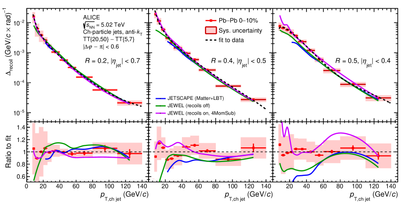
Figure 13: Upper panels: corrected $\Delta_{\mathrm{recoil}}(p_{\mathrm{T,ch~{}jet}})$ distributions measured for $R=0.2$ (left), 0.4 (middle), and 0.5 (right) in Pb–Pb collisions at $\sqrt{s_{\mathrm{NN}}}=5.02$ TeV, compared to theoretical calculations from JETSCAPE and JEWEL. Lower panels: ratio of the data and calculations to a functional fit of the measured $\Delta_{\mathrm{recoil}}(p_{\mathrm{T,ch~{}jet}})$ distributions.

Figure 13 shows the corrected $\Delta_{\mathrm{recoil}}(p_{\mathrm{T,ch~{}jet}})$ distributions measured in Pb–Pb collisions at $\sqrt{s_{\mathrm{NN}}}=5.02$ TeV, with comparison to theoretical calculations from JETSCAPE and JEWEL (both recoils on and recoils off). JETSCAPE reproduces the measurements well over the full $p_{\mathrm{T,ch~{}jet}}$ range for $R=0.2$ and 0.4, and underpredicts the data for $R=0.5$. JEWEL (recoils off) agrees with the data at high $p_{\mathrm{T,ch~{}jet}}$ for all $R$, while it underpredicts the data at low $p_{\mathrm{T,ch~{}jet}}$ for $R=0.4$ and 0.5. JEWEL (recoils on) describes the data better in the lowest $p_{\mathrm{T,ch~{}jet}}$ region of the measurement for $R=0.2$ and 0.4, while it tends to overshoot the data at low-$p_{\mathrm{T,ch~{}jet}}$ for $R=0.5$. Overall, these models provide a reasonable description of the $\Delta_{\mathrm{recoil}}(p_{\mathrm{T,ch~{}jet}})$ distribution in Pb–Pb collisions for $R=0.2$, while for $R=0.4$ and $R=0.5$, JEWEL (recoils on) best captures the main features of the data. However, none of the models quantitatively describes the data over the full $p_{\mathrm{T,ch~{}jet}}$ range for all values of $R$.

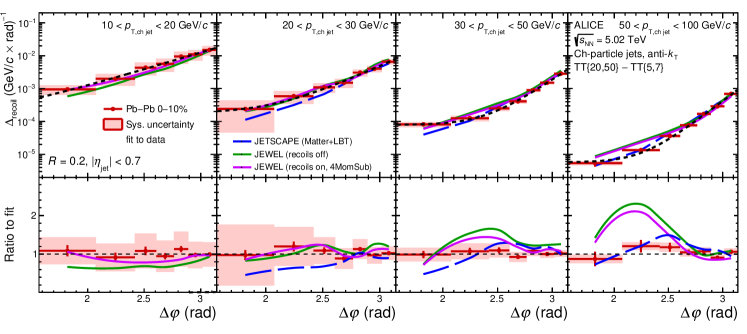
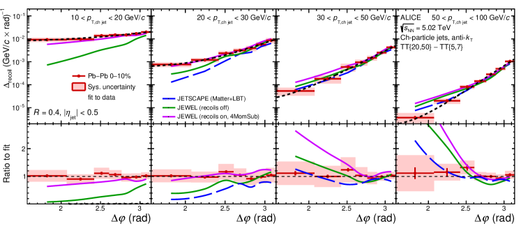
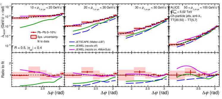
Figure 14: Corrected $\Delta_{\mathrm{recoil}}(\Delta\varphi)$ distributions for Pb–Pb collisions at $\sqrt{s_{\mathrm{NN}}}=5.02$ TeV, for $R=0.2$ (top), 0.4 (middle), and 0.5 (bottom) in $p_{\mathrm{T,ch~{}jet}}$ bins (left to right): [10,20], [20,30], [30,50], and [50,100] $\mathrm{GeV/}c$. JETSCAPE and JEWEL calculations are also shown. Upper sub-panels show the individual distributions, while lower sub-panels show their ratio to a functional fit of the data.

Figure 14 shows the corrected $\Delta_{\mathrm{recoil}}(\Delta\varphi)$ distributions for Pb–Pb collisions at $\sqrt{s_{\mathrm{NN}}}=5.02$ TeV for $R=0.2$, 0.4, and 0.5 in selected $p_{\mathrm{T,ch~{}jet}}$ bins, with comparison to model calculations. JETSCAPE describes the $\Delta\varphi$ distributions fairly well in the ranges $p_{\mathrm{T,ch~{}jet}}>20$ $\mathrm{GeV/}c$ for $R=0.2$ and $p_{\mathrm{T,ch~{}jet}}>30$ $\mathrm{GeV/}c$ for $R=0.4$, underpredicting the data in $20<p_{\mathrm{T,ch~{}jet}}<30$ $\mathrm{GeV/}c$ for $R=0.4$ and $p_{\mathrm{T,ch~{}jet}}>20$ $\mathrm{GeV/}c$ for $R=0.5$. JEWEL (recoils off) describes the data well only for $10<p_{\mathrm{T,ch~{}jet}}<30$ $\mathrm{GeV/}c$ for $R=0.2$ and $50<p_{\mathrm{T,ch~{}jet}}<100$ $\mathrm{GeV/}c$ for $R=0.5$, with poorer agreement in all other panels. JEWEL (recoils on) describes the data well except for the range $30<p_{\mathrm{T,ch~{}jet}}<100$ $\mathrm{GeV/}c$ for $R=0.2$ and 0.4.

Overall, JETSCAPE provides the best description of the data for high $p_{\mathrm{T,ch~{}jet}}$ and small $R$. JEWEL (recoils on) does best for low $p_{\mathrm{T,ch~{}jet}}$ and large $R$, while JEWEL (recoils off) and JETSCAPE significantly underestimate the tails of these distributions. These features indicate that the observable is sensitive to treatment of the medium response, which differs between the models. Further insight into in-medium jet modification can be gained by direct comparison of the Pb–Pb and $\mathrm{pp}$ distributions, which is presented next.

10.3 ${I}_{\rm AA}(p_{\mathrm{T,ch~{}jet}})$

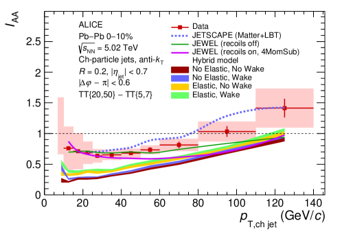
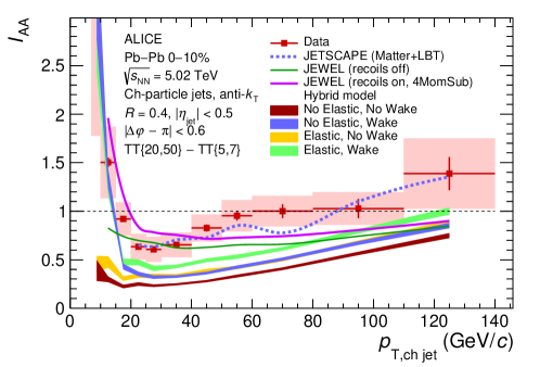
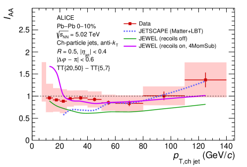
Figure 15: ${I}_{\rm AA}(p_{\mathrm{T,ch~{}jet}})$ from the $\Delta_{\mathrm{recoil}}(p_{\mathrm{T,jet}})$ distributions measured for $R=0.2$ (top), 0.4 (middle), and 0.5 (bottom) in central Pb–Pb (Fig. 13) and $\mathrm{pp}$ collisions (Fig. 11). JETSCAPE, JEWEL, and the Hybrid Model calculations are also shown.

Medium-induced yield modification is measured by ${I}_{\rm AA}(p_{\mathrm{T,ch~{}jet}})=\Delta_{\mathrm{recoil}}(\mbox{Pb--Pb})/\Delta_{\mathrm{recoil}}(\mathrm{pp})$, the ratio of the $\Delta_{\mathrm{recoil}}(p_{\mathrm{T,jet}})$ distributions measured in Pb–Pb and $\mathrm{pp}$ collisions. Figure 15 shows ${I}_{\rm AA}(p_{\mathrm{T,ch~{}jet}})$, determined using the $\Delta_{\mathrm{recoil}}(p_{\mathrm{T,ch~{}jet}})$ measurements in Figs. 11 and 13.

The ${I}_{\rm AA}(p_{\mathrm{T,ch~{}jet}})$ distributions have significant dependence on $p_{\mathrm{T,ch~{}jet}}$ and $R$. For $p_{\mathrm{T,ch~{}jet}}<20$ $\mathrm{GeV/}c$, ${I}_{\rm AA}(p_{\mathrm{T,ch~{}jet}})$ either increases above or is consistent with unity for all $R$. For $R=0.2$ and 0.4, ${I}_{\rm AA}(p_{\mathrm{T,ch~{}jet}})$ is lower than unity in the region $20<p_{\mathrm{T,ch~{}jet}}<60$ $\mathrm{GeV/}c$, corresponding to medium-induced yield suppression due to energy loss, rising towards larger $p_{\mathrm{T,ch~{}jet}}$. In contrast, ${I}_{\rm AA}(p_{\mathrm{T,ch~{}jet}})$ for $R=0.5$ is consistent with unity over the range $7<p_{\mathrm{T,ch~{}jet}}<110$ $\mathrm{GeV/}c$, indicating that the angular scale of medium-induced energy loss is less than 0.5 rad.

The JETSCAPE calculation describes well the measured ${I}_{\rm AA}(p_{\mathrm{T,ch~{}jet}})$ distributions for $R=0.2$ and 0.4 in $p_{\mathrm{T,ch~{}jet}}>20$ $\mathrm{GeV/}c$, including the rising trend for $p_{\mathrm{T,ch~{}jet}}>60$ $\mathrm{GeV/}c$. JETSCAPE predicts a similar $p_{\mathrm{T,ch~{}jet}}$-dependence of ${I}_{\rm AA}(p_{\mathrm{T,ch~{}jet}})$ for $R=0.5$, which however is not consistent with the measurement.

The JEWEL calculations, both recoils-off and recoils-on, describe the ${I}_{\rm AA}(p_{\mathrm{T,ch~{}jet}})$ distribution for $R=0.2$ at low $p_{\mathrm{T,ch~{}jet}}$, but do not capture the $p_{\mathrm{T,ch~{}jet}}$ dependence of the data and underpredict them at higher $p_{\mathrm{T,ch~{}jet}}$. For $R=0.4$, both versions underestimate the data at high $p_{\mathrm{T,ch~{}jet}}$. For $R=0.4$ and 0.5, JEWEL (recoils on) shows a significant increase in ${I}_{\rm AA}(p_{\mathrm{T,ch~{}jet}})$ towards low $p_{\mathrm{T,ch~{}jet}}$ for $p_{\mathrm{T,ch~{}jet}}<20~{}\mathrm{GeV/}c$, similar to the trend in the data for $R=0.4$. This increase is not seen for recoils-off. The larger value of ${I}_{\rm AA}(p_{\mathrm{T,ch~{}jet}})$ in $20<p_{\mathrm{T,ch~{}jet}}<60$ $\mathrm{GeV/}c$ for $R=0.5$ seen in the data is reproduced by JEWEL with recoils-on but not recoils-off. This $R$-dependence is due to the implementation of medium response in JEWEL, in which energy is carried by recoiling partons at large angles to the jet centroid [81].

Hybrid Model calculations of ${I}_{\rm AA}(p_{\mathrm{T,ch~{}jet}})$ are presented for $R=0.2$ and 0.4. The model underestimates the magnitude of the data for all settings, although it reproduces the rising trend with increasing $p_{\mathrm{T,ch~{}jet}}$ seen in the data for $p_{\mathrm{T,ch~{}jet}}>20$ $\mathrm{GeV/}c$. The model likewise captures the sharply rising trend with decreasing $p_{\mathrm{T,ch~{}jet}}$ at low $p_{\mathrm{T,ch~{}jet}}$ for $R=0.4$ with wake turned on, while no rising trend is seen when the wake is turned off, independent of the elastic scattering component.

Overall, JETSCAPE most accurately describes both the magnitude and $p_{\mathrm{T,ch~{}jet}}$ dependence of ${I}_{\rm AA}(p_{\mathrm{T,ch~{}jet}})$ in the range $p_{\mathrm{T,ch~{}jet}}>20$ $\mathrm{GeV/}c$ for $R=0.2$ and $R=0.4$, while JEWEL most accurately describes it in the same $p_{\mathrm{T,ch~{}jet}}$ region for $R=0.5$. The rising trend in data towards low $p_{\mathrm{T,ch~{}jet}}$ for $p_{\mathrm{T,ch~{}jet}}<20$ $\mathrm{GeV/}c$ is described by both the Hybrid Model and JEWEL, but only with the inclusion of medium-response effects.

10.4 ${I}_{\rm AA}(p_{\mathrm{T,ch~{}jet}})$ and trigger bias

A common picture of inclusive high-$p_{\mathrm{T}}$ hadron production in the presence of jet quenching in central A–A collisions is that the geometric distribution of vertices which generate such hadrons is biased, due to the interplay of jet energy loss and the shapes of the jet $p_{\mathrm{T}}$ spectrum and fragmentation function [43, 44, 45, 46, 50]. In this picture, observed high-$p_{\mathrm{T}}$ hadrons arise predominantly from jets generated in hard partonic scattering processes occuring at the surface of the hot QGP, headed outward (“surface bias”). For the semi-inclusive observable in this measurement, this surface bias implies a longer average path length for the jet population recoiling from a high-$p_{\mathrm{T}}$ hadron trigger than for the unbiased inclusive jet population.

This analysis indeed selects events based on the presence of a trigger hadron, which is a leading fragment of a “trigger” jet. To characterize this measurement the observable $\tilde{z}$ is defined as

$$\tilde{z}=\frac{p_{\mathrm{T}}^{\mathrm{trig}}}{p_{\mathrm{T,ch~{}jet}}},$$ (6)

which is the ratio between the trigger hadron $p_{\mathrm{T}}$ and the recoiling charged-particle jet $p_{\mathrm{T}}$. Dijet production at LO is a $2\rightarrow 2$ process, generating a jet pair that is azimuthally back-to-back at the same value of $p_{\mathrm{T,ch~{}jet}}$. If LO processes dominate hadron production, and the measurement includes the full (rather than charged-particle) energy of the recoil jet, then $\tilde{z}<1$ for all jets contributing to the ${I}_{\rm AA}$ distribution. However, higher-order processes are in general not negligible, and the recoil jets in this measurement are based on charged particles only. Initial-state $k_{\mathrm{T}}$ effects can also modify $\tilde{z}$. Nevertheless, $\tilde{z}$ provides a useful qualitative categorization of different kinematic regions in Fig. 15.

The surface-bias argument outlined above is based on the shape of the high-$z$ (high momentum fraction) tail of the fragmentation function. However, for $p_{\mathrm{T}}^{\mathrm{trig}}=20$ $\mathrm{GeV/}c$, which is the lower bound of the $\mathrm{TT}_{\mathrm{sig}}$ trigger interval $\mathrm{TT}\{20,50\}$, $p_{\mathrm{T,ch~{}jet}}=100$ $\mathrm{GeV/}c$ corresponds to $\tilde{z}=0.2$, and its value would be yet smaller if the fully-reconstructed jet energy were used. It is evident that, for events containing jets that contribute to the highest $p_{\mathrm{T,ch~{}jet}}$ bins in Fig. 15, the assumptions underlying the surface-bias argument may not pertain; in particular, the trigger hadron that satisfies the $\mathrm{TT}\{20,50\}$ selection may not be a leading fragment of its parent (“trigger”) jet.

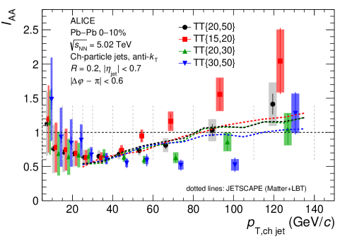
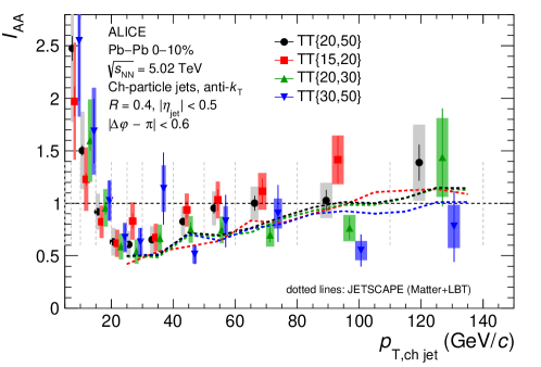
Figure 16: ${I}_{\rm AA}(p_{\mathrm{T,ch~{}jet}})$ for $R=0.2$ and 0.4, for various $\mathrm{TT}_{\mathrm{sig}}$ selections. The data points have been displaced for clarity, and the vertical dashed grey lines indicate the bin edges. JETSCAPE predictions for the corresponding $\mathrm{TT}_{\mathrm{sig}}$ selections are also shown.

Further insight into the rising trend of ${I}_{\rm AA}(p_{\mathrm{T,ch~{}jet}})$ at large $p_{\mathrm{T,ch~{}jet}}$ seen in Fig. 15 can be obtained by varying the hadron trigger $p_{\mathrm{T}}$ range for the $\mathrm{TT}_{\mathrm{sig}}$-selected event population, i.e. by varying the distribution of $\tilde{z}$ for fixed recoil $p_{\mathrm{T,ch~{}jet}}$. Figure 16 shows the ${I}_{\rm AA}(p_{\mathrm{T,ch~{}jet}})$ distribution for $R=0.2$ and 0.4 measured for several choices of $p_{\mathrm{T}}^{\mathrm{trig}}$ interval for the $\mathrm{TT}_{\mathrm{sig}}$ event selection. A higher $p_{\mathrm{T}}^{\mathrm{trig}}$ threshold corresponds to larger $\tilde{z}$, where the assumptions underlying the surface-bias picture may better apply. The results show that, as the lower $p_{\mathrm{T}}^{\mathrm{trig}}$ bound is raised, the rate of increase in ${I}_{\rm AA}(p_{\mathrm{T,ch~{}jet}})$ at large $p_{\mathrm{T,ch~{}jet}}$ diminishes.

As noted above, large $\tilde{z}$ may correspond to larger average in-medium path length of the recoiling jet, with corresponding larger recoil yield suppression due to quenching. Figure 16 shows that increasing $\tilde{z}$ indeed results in larger recoil yield suppression, consistent with this geometrical picture. The figure also shows JETSCAPE calculations, which exhibit a slightly slower rise in ${I}_{\rm AA}(p_{\mathrm{T,ch~{}jet}})$ at large $p_{\mathrm{T,ch~{}jet}}$ for higher $p_{\mathrm{T}}^{\mathrm{trig}}$ intervals (larger $\tilde{z}$), although the variation is quantitatively smaller than that seen in the data. The results in Fig. 16 provide new insight into the conjecture of surface bias for inclusive high-$p_{\mathrm{T}}$ hadron production, and the interplay of jet quenching effects as observed via hadronic and reconstructed jet observables.

10.5 Jet shape modification: $R$-dependence of $\Delta_{\mathrm{recoil}}(p_{\mathrm{T,ch~{}jet}})$

The ratio of inclusive jet cross sections or semi-inclusive jet yields at different values of $R$ provides a precise probe of jet shape, since there is significant cancellation of correlated uncertainties in the ratio for both experimental measurements and theoretical calculations  [121, 122, 123, 17]. In $\mathrm{pp}$ collisions, $R$-dependent ratios are sensitive to high-order pQCD effects [122, 124, 17, 125]. In A–A collisions, such ratios provide experimentally robust probes of medium-induced modification of jet shapes over a broad kinematic range, including low $p_{\mathrm{T,jet}}$ [50, 70, 71].

10.5.1 pp collisions

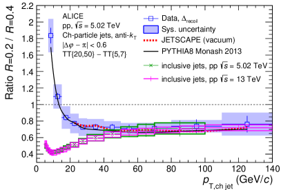
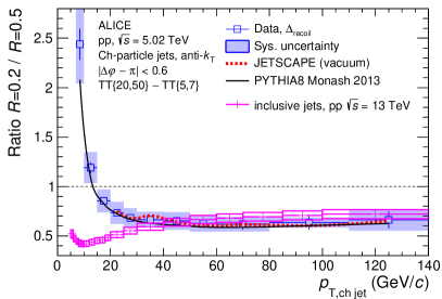
Figure 17: Ratio of $\Delta_{\mathrm{recoil}}(p_{\mathrm{T,ch~{}jet}})$ distributions in $\mathrm{pp}$ collisions at $\sqrt{s}=5.02$ TeV using the data from Fig. 11, for $R=0.2/R=0.4$ (left) and $R=0.2/R=0.5$ (right), compared to calculations from PYTHIA8 and JETSCAPE. The corresponding ratios of cross sections for inclusive jets are also shown for $\mathrm{pp}$ collisions at $\sqrt{s}=5.02$ TeV [56] and $\sqrt{s}=13$ TeV [126]. The uncertainties in the ratio take into account the correlation of uncertainties between numerator and denominator.

Figure 17 shows the ratio of $\Delta_{\mathrm{recoil}}(p_{\mathrm{T,ch~{}jet}})$ distributions for $R=0.2$ over that for $R=0.4$ or $R=0.5$ in $\mathrm{pp}$ collisions at $\sqrt{s}=5.02$ TeV, using the data in Fig. 11. The ratio is below unity for $p_{\mathrm{T,ch~{}jet}}>15$ $\mathrm{GeV/}c$, consistent with the expected intra-jet energy distribution in which significant energy is carried at distances larger than 0.2 radians relative to the jet axis. The ratio rises towards low $p_{\mathrm{T,ch~{}jet}}$ and crossing unity at $p_{\mathrm{T,ch~{}jet}}\sim 10$ $\mathrm{GeV/}c$. The measured distributions are well-reproduced by PYTHIA8 and JETSCAPE (vacuum) calculations. This $p_{\mathrm{T,ch~{}jet}}$-dependence and the good agreement of this observable with PYTHIA8 were also observed in Ref. [50], where an NLO pQCD calculation was likewise shown to reproduce the measured $p_{\mathrm{T,ch~{}jet}}$-dependence of the ratio, although not its absolute magnitude.

Figure 17 also shows the ratios of the inclusive charged-jet cross sections for different values of $R$ in $\mathrm{pp}$ collisions at $\sqrt{s}=5.02$ TeV [56] and $\sqrt{s}=13$ TeV [126]. At high $p_{\mathrm{T,ch~{}jet}}$  these ratios are consistent within uncertainties with the corresponding $\Delta_{\mathrm{recoil}}(p_{\mathrm{T,ch~{}jet}})$ ratios. However, the observed increase in the $\Delta_{\mathrm{recoil}}(p_{\mathrm{T,ch~{}jet}})$ ratio with decreasing $p_{\mathrm{T,ch~{}jet}}$ is opposite to the behavior of the ratios for inclusive jet cross sections, which decrease with decreasing $p_{\mathrm{T,ch~{}jet}}$. Note that the inclusive charged jet cross section ratios are also well-described by pQCD and Monte Carlo model calculations [56, 126]. Since PYTHIA8 accurately reproduces the $R$-dependent ratios for both populations, this difference evidently originates in QCD processes that are incorporated in PYTHIA8.

The difference in low-$p_{\mathrm{T,ch~{}jet}}$ behavior of the inclusive and coincidence channel $R$-ratios may be understood in terms of the $\tilde{z}$ observable defined in Eq. 6. Since the lower bound of the $\mathrm{TT}_{\mathrm{sig}}$ selection is $p_{\mathrm{T}}^{\mathrm{trig}}=20$ $\mathrm{GeV/}c$, the region $p_{\mathrm{T,ch~{}jet}}<20$ $\mathrm{GeV/}c$ in Fig. 17 corresponds to $\tilde{z}>1$, where LO processes are suppressed and jet production is dominated by higher-order processes that incorporate hard gluon radiation. For an NLO process in which hard radiation is emitted at angles $\sim 0.2-0.4$ rad relative to the jet axis, jet reconstruction may result in two rather than one jet (jet splitting) preferentially for $R=0.2$ relative to $R=0.4$. In this semi-inclusive analysis, in which the number of jets in a triggered event is simply counted, such splittings will enhance the $R$-dependent $\Delta_{\mathrm{recoil}}(p_{\mathrm{T,jet}})$ ratio at low $p_{\mathrm{T,ch~{}jet}}$, consistent with Fig. 17. The inclusive population is not subject to a bias like that induced by $p_{\mathrm{T}}^{\mathrm{trig}}$ for the coincidence population, and its $R$-dependent inclusive cross section ratio at low $p_{\mathrm{T,jet}}$ therefore reflects the ensemble-averaged shape of the unbiased jet distribution.

This picture can be further explored using model calculations. If LO production processes indeed are suppressed in the phase space $\tilde{z}>1$, this may provide a new tool for controlled generation of a population of “wide” jets, which are predicted to interact differently on average with the QGP as compared to a more inclusive population [127].

10.5.2 Pb–Pb collisions

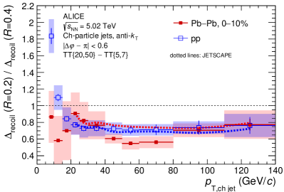
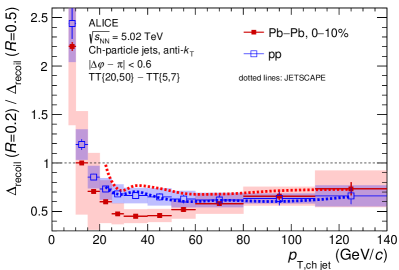
Figure 18: Ratio of $\Delta_{\mathrm{recoil}}(p_{\mathrm{T,ch~{}jet}})$ distributions with different $R$ for Pb–Pb collisions at $\sqrt{s_{\mathrm{NN}}}=5.02$ TeV from the data in Fig. 13, together with the ratios for $\mathrm{pp}$ collisions from Fig. 17, for $R=0.2/R=0.4$ (left) and $R=0.2/R=0.5$ (right). The uncertainty in the ratio takes into account the correlation of uncertainties between numerator and denominator. JETSCAPE calculations for $\mathrm{pp}$ and Pb–Pb collisions are also shown.

Figure 18 shows the $R$-dependent ratio of $\Delta_{\mathrm{recoil}}(p_{\mathrm{T,ch~{}jet}})$ distributions for Pb–Pb collisions at $\sqrt{s_{\mathrm{NN}}}=5.02$ TeV, using the data from Fig. 13, compared to the same ratios for $\mathrm{pp}$ collisions shown in Fig. 17. At intermediate values of $p_{\mathrm{T,ch~{}jet}}$ the ratios for Pb–Pb collisions are lower than those for $\mathrm{pp}$ collisions, indicating significant medium-induced intra-jet broadening in that region. However, the results of JETSCAPE calculations incorporating jet quenching in Pb–Pb collisions are larger than those in $\mathrm{pp}$ collisions, in contrast to the data. This indicates that medium-induced intra-jet broadening is not accurately modeled in JETSCAPE.

The medium-induced suppression of the $R$-dependent ratio in Fig. 18, corresponding to medium-induced intra-jet broadening, is in contrast to a similar measurement of the inclusive jet population [72] which finds medium-induced jet narrowing in a similar kinematic range. The jet populations of these two measurements differ, however, and they cannot be compared directly. Exploration of this difference requires the calculation of both observables within the same model framework.

10.6 Acoplanarity

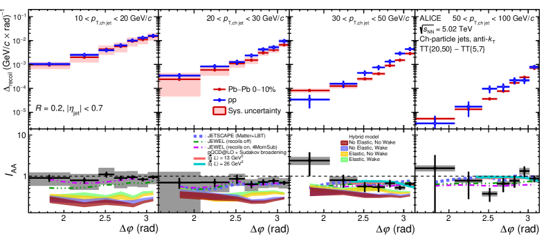
Figure 19: Distributions as a function of $\Delta\varphi$ for $R=0.2$. Upper panels: $\Delta_{\mathrm{recoil}}(\Delta\varphi)$ in intervals of $p_{\mathrm{T,ch~{}jet}}$ measured in $\mathrm{pp}$ and Pb–Pb collisions. Lower panels: ${I}_{\rm AA}(p_{\mathrm{T,ch~{}jet}})$, the ratio of the $\mathrm{pp}$ and Pb–Pb distributions in the corresponding upper panel. Predictions from JETSCAPE, JEWEL, Hybrid model, and a pQCD calculation are also shown.

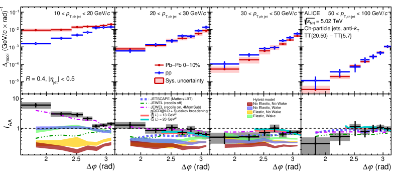
Figure 20: Same as Fig. 19, for $R=0.4$.

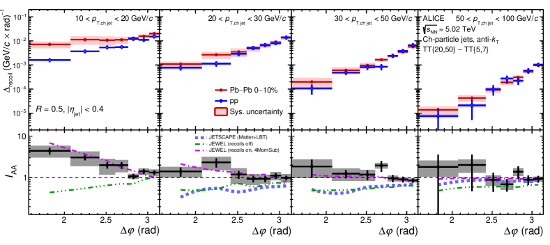
Figure 21: Same as Fig. 19, for $R=0.5$.

Figures 19, 20, and 21 show $\Delta_{\mathrm{recoil}}(\Delta\varphi)$ (acoplanarity) distributions measured in different $p_{\mathrm{T,ch~{}jet}}$ intervals for $\mathrm{pp}$ and Pb–Pb collisions, together with their ratio ${I}_{\rm AA}(\Delta\varphi)$, for $R=0.2,0.4$, and $0.5$, respectively. The key physics conclusions from these results, including phenomenological discussion and model comparisons for $R=0.4$, are presented in the companion Letter [75]. This paper additionally reports acoplanarity distributions in the range $50<p_{\mathrm{T,ch~{}jet}}<100$ $\mathrm{GeV/}c$, and comparison to model calculations for $R=0.2$ and $R=0.5$.

Suppression of ${I}_{\rm AA}(\Delta\varphi)$ below unity can be seen in some $p_{\mathrm{T,ch~{}jet}}$ regions, consistent with the yield suppression in Fig. 15. In the range $p_{\mathrm{T,ch~{}jet}}>10$ $\mathrm{GeV/}c$ for $R=0.2$, and the range $p_{\mathrm{T,ch~{}jet}}>20$ $\mathrm{GeV/}c$ for $R=0.4$ and $R=0.5$, the shape of the Pb–Pb $\Delta_{\mathrm{recoil}}(\Delta\varphi)$ distributions are consistent with that of the $\mathrm{pp}$ distributions, corresponding to no significant in-medium acoplanarity broadening within the experimental uncertainties. In contrast, significant enhancement in ${I}_{\rm AA}(\Delta\varphi)$ at $\Delta\varphi$ values far from $\pi$ is observed in the region $10<p_{\mathrm{T,ch~{}jet}}<20$ $\mathrm{GeV/}c$  for $R=0.4$ and 0.5, corresponding to medium-induced broadening of the acoplanarity distribution.

While these figures present fully-corrected distributions in regions of small signal to background at low $p_{\mathrm{T,ch~{}jet}}$, it is important to determine whether significant correlated signal in these regions is already evident in the raw data distributions, and is not introduced primarily by the correction procedures. This point is discussed in Sec. 4.3. As an additional cross check, the $\mathrm{pp}$ unfolded distributions were folded with the Pb–Pb response and compared to the corresponding raw Pb–Pb distributions. Significant broadening of the $\Delta\varphi$ distribution with respect to this reference was also observed at low $p_{\mathrm{T,ch~{}jet}}$.

Figures 19, 20, and 21 also compare the measured ${I}_{\rm AA}(\Delta\varphi)$ to theoretical calculations. The JETSCAPE calculation describes the $R=0.2$ data for $p_{\mathrm{T,ch~{}jet}}>20$ $\mathrm{GeV/}c$, where the results of the calculation are available, while it underestimates the $R=0.4$ data for $20<p_{\mathrm{T,ch~{}jet}}<30$ $\mathrm{GeV/}c$ and $R=0.5$ data for $20<p_{\mathrm{T,ch~{}jet}}<50$ $\mathrm{GeV/}c$, with larger discrepancy farther from $\Delta\varphi=\pi$. The JEWEL calculation (both options) also describes the $R=0.2$ data for all $p_{\mathrm{T,ch~{}jet}}$ intervals, with minimal difference between recoils-on and recoils-off. For larger $R$, JEWEL (recoils on) describes the data for all $p_{\mathrm{T,ch~{}jet}}$ intervals and jet $R$, while JEWEL (recoils off) significantly underpredicts the data in the region $p_{\mathrm{T,jet}}<20$ $\mathrm{GeV/}c$ for $R=0.4$ and $p_{\mathrm{T,jet}}<50$ $\mathrm{GeV/}c$ for $R=0.5$, most significantly in the tails of the distributions. The Hybrid model underpredicts the magnitude of the ${I}_{\rm AA}(\Delta\varphi)$ for $R=0.2$ and $R=0.4$, for all model settings. The inclusion of wake effects increases the ${I}_{\rm AA}(\Delta\varphi)$ at low $p_{\mathrm{T,ch~{}jet}}$ for $R=0.2$ and $R=0.4$, while the inclusion of elastic scattering moderately increases the prediction close to $\Delta\varphi=\pi$ in all $p_{\mathrm{T,ch~{}jet}}$ intervals for $R=0.2$, and for $p_{\mathrm{T,ch~{}jet}}>20$ $\mathrm{GeV/}c$ for $R=0.4$, bringing the predictions closer to data. However, the significant azimuthal broadening seen at low $p_{\mathrm{T,ch~{}jet}}$ for $R=0.4$ is not reproduced. The pQCD calculations at LO reproduce the measured ${I}_{\rm AA}(p_{\mathrm{T,ch~{}jet}})$ distributions in the range $p_{\mathrm{T,ch~{}jet}}>20$ $\mathrm{GeV/}c$ for $R=0.2$ and 0.4, though over a restricted range in acoplanarity, $2.4<\Delta\varphi<\pi$. The data do not discriminate between the two values of quenching parameter in calculation, $\langle\hat{q}L\rangle=$ 13 and 26 GeV². A higher-order calculation is required to extend the range of $\Delta\varphi$, with correspondingly greater discrimination of quenching parameters.

Overall, JEWEL (recoils on) describes the data the best over the full $R$ and $p_{\mathrm{T,ch~{}jet}}$ range, including the significant azimuthal broadening for low $p_{\mathrm{T,ch~{}jet}}$ and large $R$. However, none of the models considered successfully describes the full set of measured data. The physics consequences of the systematic dependencies of medium-induced effects on $p_{\mathrm{T,ch~{}jet}}$ and $R$, and the comparison of models to these data, are discussed in Ref. [75]

11 Summary and Outlook

This paper reports measurements of semi-inclusive distributions of charged-particle jets recoiling from a high-$p_{\mathrm{T}}$ hadron trigger in $\mathrm{pp}$ and central Pb–Pb collisions at $\sqrt{s_{\mathrm{NN}}}=5.02$ TeV, using the large data samples recorded with the ALICE detector during LHC Run 2. The results are reported as a function of both $p_{\mathrm{T,jet}}$, the recoil jet transverse momentum, and $\Delta\varphi$, the azimuthal separation between the trigger and recoil jet. A statistical, data-driven method previously developed by the ALICE Collaboration is used to mitigate the large uncorrelated background jet yield in central Pb–Pb collisions, enabling measurements of jet quenching in a kinematic region previously unexplored by reconstructed jets at the LHC, including low $p_{\mathrm{T,jet}}\sim 10$ $\mathrm{GeV/}c$ with jet resolution parameter $R=0.5$. The observed phenomena explore several different aspects of jet production in $\mathrm{pp}$ and Pb–Pb collisions.

The $p_{\mathrm{T,jet}}$ and azimuthal distributions measured in $\mathrm{pp}$ collisions provide a precise reference to explore medium-induced modifications to jet production in central Pb–Pb collisions, and are well described by pQCD-based calculations over the entire measured ranges. The ratio of recoil jet yields in $\mathrm{pp}$ collisions for $R=0.2$ to that for $R=0.4$ or 0.5 is below unity at high $p_{\mathrm{T}}$, reflecting the well-established transverse profile of energy within a jet in vacuum. However, this ratio is observed to increase as $p_{\mathrm{T,jet}}$ is reduced below the value of $p_{\mathrm{T}}^{\mathrm{trig}}$, the trigger hadron $p_{\mathrm{T}}$, in marked contrast to the behavior of a similar ratio measured for inclusive jet cross sections. Both sets of measurements are well described by pQCD calculations, suggesting that these opposing effects may arise from different jet production mechanisms, in particular suppression of leading order processes for the semi-inclusive population of jets recoiling from a high-$p_{\mathrm{T}}$ hadron trigger, in which $p_{\mathrm{T}}^{\mathrm{trig}}$ provides an additional scale.

The measured values of ${I}_{\rm AA}(p_{\mathrm{T,ch~{}jet}})$, the ratio of recoil yield for Pb–Pb and $\mathrm{pp}$ collisions for the same jet $R$ as a function of $p_{\mathrm{T,ch~{}jet}}$, exhibit a dependence on $p_{\mathrm{T,jet}}$ and $R$. For $R=0.5$, the ratio is consistent with unity within uncertainties over the entire measured range, indicating that medium-induced jet modifications as probed by this observable are largely constrained to angular scales less than 0.5 radians. The ratio of recoil jet yield in Pb–Pb collisions for $R=0.2$ to that for $R=0.4$ or 0.5 is below that for $\mathrm{pp}$ collisions at intermediate $p_{\mathrm{T,jet}}$, indicating medium-induced intra-jet broadening within this angular scale.

For $R=0.2$ and 0.4, the value of ${I}_{\rm AA}(p_{\mathrm{T,ch~{}jet}})$ is below unity at intermediate $p_{\mathrm{T,jet}}$, increasing to unity at both lower and higher $p_{\mathrm{T,jet}}$. For $R=0.4$, ${I}_{\rm AA}(p_{\mathrm{T,ch~{}jet}})$ exceeds unity at the lowest value of $p_{\mathrm{T,jet}}$ reported here. Comparison to models indicates that the low-$p_{\mathrm{T,jet}}$ behavior may be due to the recovery of energy lost to the medium by higher-$p_{\mathrm{T,jet}}$ jets that are likewise correlated with the trigger. The high-$p_{\mathrm{T,jet}}$ behavior may arise from the interplay between the energy loss due to jet quenching and the geometric bias induced by using a hadron trigger.

The measured values of ${I}_{\rm AA}(\Delta\varphi)$, the ratio of recoil yield for Pb–Pb and $\mathrm{pp}$ collisions for the same jet $R$ as a function of $\Delta\varphi$, provide the first measurement of significant in-medium jet acoplanarity broadening in Pb–Pb collisions, for $R=0.4$ and 0.5 at low $p_{\mathrm{T,ch~{}jet}}$.

These measurements and model calculations are discussed further in the companion Letter. Global analyses incorporating these data will enable quantitative, multi-messenger studies to further elucidate the nature of the QGP as probed by jets.

Appendix A The ALICE Collaboration

S. Acharya  ¹²⁶, D. Adamová  ⁸⁶, G. Aglieri Rinella  ³³, M. Agnello  ³⁰, N. Agrawal  ⁵¹, Z. Ahammed  ¹³⁴, S. Ahmad¹⁶, S.U. Ahn  ⁷¹, I. Ahuja  ³⁸, A. Akindinov  ¹⁴², M. Al-Turany  ⁹⁷, D. Aleksandrov  ¹⁴², B. Alessandro  ⁵⁶, H.M. Alfanda  ⁶, R. Alfaro Molina  ⁶⁷, B. Ali  ¹⁶, A. Alici  ²⁶, N. Alizadehvandchali  ¹¹⁵, A. Alkin  ³³, J. Alme  ²¹, G. Alocco  ⁵², T. Alt  ⁶⁴, A.R. Altamura  ⁵⁰, I. Altsybeev  ⁹⁵, M.N. Anaam  ⁶, C. Andrei  ⁴⁶, N. Andreou  ¹¹⁴, A. Andronic  ¹³⁷, V. Anguelov  ⁹⁴, F. Antinori  ⁵⁴, P. Antonioli  ⁵¹, N. Apadula  ⁷⁴, L. Aphecetche  ¹⁰³, H. Appelshäuser  ⁶⁴, C. Arata  ⁷³, S. Arcelli  ²⁶, M. Aresti  ²³, R. Arnaldi  ⁵⁶, J.G.M.C.A. Arneiro  ¹¹⁰, I.C. Arsene  ²⁰, M. Arslandok  ¹³⁹, A. Augustinus  ³³, R. Averbeck  ⁹⁷, M.D. Azmi¹⁶, H. Baba¹²³, A. Badalà  ⁵³, J. Bae  ¹⁰⁴, Y.W. Baek  ⁴¹, X. Bai  ¹¹⁹, R. Bailhache  ⁶⁴, Y. Bailung  ⁴⁸, A. Balbino  ³⁰, A. Baldisseri  ¹²⁹, B. Balis  ², D. Banerjee  ⁴, Z. Banoo  ⁹¹, R. Barbera  ²⁷, F. Barile  ³², L. Barioglio  ⁹⁵, M. Barlou⁷⁸, B. Barman⁴², G.G. Barnaföldi  ¹³⁸, L.S. Barnby  ⁸⁵, V. Barret  ¹²⁶, L. Barreto  ¹¹⁰, C. Bartels  ¹¹⁸, K. Barth  ³³, E. Bartsch  ⁶⁴, N. Bastid  ¹²⁶, S. Basu  ⁷⁵, G. Batigne  ¹⁰³, D. Battistini  ⁹⁵, B. Batyunya  ¹⁴³, D. Bauri⁴⁷, J.L. Bazo Alba  ¹⁰¹, I.G. Bearden  ⁸³, C. Beattie  ¹³⁹, P. Becht  ⁹⁷, D. Behera  ⁴⁸, I. Belikov  ¹²⁸, A.D.C. Bell Hechavarria  ¹³⁷, F. Bellini  ²⁶, R. Bellwied  ¹¹⁵, S. Belokurova  ¹⁴², Y.A.V. Beltran  ⁴⁵, G. Bencedi  ¹³⁸, S. Beole  ²⁵, Y. Berdnikov  ¹⁴², A. Berdnikova  ⁹⁴, L. Bergmann  ⁹⁴, M.G. Besoiu  ⁶³, L. Betev  ³³, P.P. Bhaduri  ¹³⁴, A. Bhasin  ⁹¹, M.A. Bhat  ⁴, B. Bhattacharjee  ⁴², L. Bianchi  ²⁵, N. Bianchi  ⁴⁹, J. Bielčík  ³⁶, J. Bielčíková  ⁸⁶, J. Biernat  ¹⁰⁷, A.P. Bigot  ¹²⁸, A. Bilandzic  ⁹⁵, G. Biro  ¹³⁸, S. Biswas  ⁴, N. Bize  ¹⁰³, J.T. Blair  ¹⁰⁸, D. Blau  ¹⁴², M.B. Blidaru  ⁹⁷, N. Bluhme³⁹, C. Blume  ⁶⁴, G. Boca  ^22,55, F. Bock  ⁸⁷, T. Bodova  ²¹, A. Bogdanov¹⁴², S. Boi  ²³, J. Bok  ⁵⁸, L. Boldizsár  ¹³⁸, M. Bombara  ³⁸, P.M. Bond  ³³, G. Bonomi  ^133,55, H. Borel  ¹²⁹, A. Borissov  ¹⁴², A.G. Borquez Carcamo  ⁹⁴, H. Bossi  ¹³⁹, E. Botta  ²⁵, Y.E.M. Bouziani  ⁶⁴, L. Bratrud  ⁶⁴, P. Braun-Munzinger  ⁹⁷, M. Bregant  ¹¹⁰, M. Broz  ³⁶, G.E. Bruno  ^96,32, M.D. Buckland  ²⁴, D. Budnikov  ¹⁴², H. Buesching  ⁶⁴, S. Bufalino  ³⁰, P. Buhler  ¹⁰², N. Burmasov  ¹⁴², Z. Buthelezi  ^68,122, A. Bylinkin  ²¹, S.A. Bysiak¹⁰⁷, M. Cai  ⁶, H. Caines  ¹³⁹, A. Caliva  ²⁹, E. Calvo Villar  ¹⁰¹, J.M.M. Camacho  ¹⁰⁹, P. Camerini  ²⁴, F.D.M. Canedo  ¹¹⁰, M. Carabas  ¹²⁵, A.A. Carballo  ³³, F. Carnesecchi  ³³, R. Caron  ¹²⁷, L.A.D. Carvalho  ¹¹⁰, J. Castillo Castellanos  ¹²⁹, F. Catalano  ^33,25, C. Ceballos Sanchez  ¹⁴³, I. Chakaberia  ⁷⁴, P. Chakraborty  ⁴⁷, S. Chandra  ¹³⁴, S. Chapeland  ³³, M. Chartier  ¹¹⁸, S. Chattopadhyay  ¹³⁴, S. Chattopadhyay  ⁹⁹, T.G. Chavez  ⁴⁵, T. Cheng  ^97,6, C. Cheshkov  ¹²⁷, B. Cheynis  ¹²⁷, V. Chibante Barroso  ³³, D.D. Chinellato  ¹¹¹, E.S. Chizzali  ^I,95, J. Cho  ⁵⁸, S. Cho  ⁵⁸, P. Chochula  ³³, D. Choudhury⁴², P. Christakoglou  ⁸⁴, C.H. Christensen  ⁸³, P. Christiansen  ⁷⁵, T. Chujo  ¹²⁴, M. Ciacco  ³⁰, C. Cicalo  ⁵², F. Cindolo  ⁵¹, M.R. Ciupek⁹⁷, G. Clai^II,51, F. Colamaria  ⁵⁰, J.S. Colburn¹⁰⁰, D. Colella  ^96,32, M. Colocci  ²⁶, M. Concas  ^III,33, G. Conesa Balbastre  ⁷³, Z. Conesa del Valle  ¹³⁰, G. Contin  ²⁴, J.G. Contreras  ³⁶, M.L. Coquet  ¹²⁹, P. Cortese  ^132,56, M.R. Cosentino  ¹¹², F. Costa  ³³, S. Costanza  ^22,55, C. Cot  ¹³⁰, J. Crkovská  ⁹⁴, P. Crochet  ¹²⁶, R. Cruz-Torres  ⁷⁴, P. Cui  ⁶, A. Dainese  ⁵⁴, M.C. Danisch  ⁹⁴, A. Danu  ⁶³, P. Das  ⁸⁰, P. Das  ⁴, S. Das  ⁴, A.R. Dash  ¹³⁷, S. Dash  ⁴⁷, R.M.H. David⁴⁵, A. De Caro  ²⁹, G. de Cataldo  ⁵⁰, J. de Cuveland³⁹, A. De Falco  ²³, D. De Gruttola  ²⁹, N. De Marco  ⁵⁶, C. De Martin  ²⁴, S. De Pasquale  ²⁹, R. Deb  ¹³³, R. Del Grande  ⁹⁵, L. Dello Stritto  ²⁹, W. Deng  ⁶, P. Dhankher  ¹⁹, D. Di Bari  ³², A. Di Mauro  ³³, B. Diab  ¹²⁹, R.A. Diaz  ^143,7, T. Dietel  ¹¹³, Y. Ding  ⁶, J. Ditzel  ⁶⁴, R. Divià  ³³, D.U. Dixit  ¹⁹, Ø. Djuvsland²¹, U. Dmitrieva  ¹⁴², A. Dobrin  ⁶³, B. Dönigus  ⁶⁴, J.M. Dubinski  ¹³⁵, A. Dubla  ⁹⁷, S. Dudi  ⁹⁰, P. Dupieux  ¹²⁶, M. Durkac¹⁰⁶, N. Dzalaiova¹³, T.M. Eder  ¹³⁷, R.J. Ehlers  ⁷⁴, F. Eisenhut  ⁶⁴, R. Ejima⁹², D. Elia  ⁵⁰, B. Erazmus  ¹⁰³, F. Ercolessi  ²⁶, B. Espagnon  ¹³⁰, G. Eulisse  ³³, D. Evans  ¹⁰⁰, S. Evdokimov  ¹⁴², L. Fabbietti  ⁹⁵, M. Faggin  ²⁸, J. Faivre  ⁷³, F. Fan  ⁶, W. Fan  ⁷⁴, A. Fantoni  ⁴⁹, M. Fasel  ⁸⁷, A. Feliciello  ⁵⁶, G. Feofilov  ¹⁴², A. Fernández Téllez  ⁴⁵, L. Ferrandi  ¹¹⁰, M.B. Ferrer  ³³, A. Ferrero  ¹²⁹, C. Ferrero  ⁵⁶, A. Ferretti  ²⁵, V.J.G. Feuillard  ⁹⁴, V. Filova  ³⁶, D. Finogeev  ¹⁴², F.M. Fionda  ⁵², E. Flatland³³, F. Flor  ¹¹⁵, A.N. Flores  ¹⁰⁸, S. Foertsch  ⁶⁸, I. Fokin  ⁹⁴, S. Fokin  ¹⁴², E. Fragiacomo  ⁵⁷, E. Frajna  ¹³⁸, U. Fuchs  ³³, N. Funicello  ²⁹, C. Furget  ⁷³, A. Furs  ¹⁴², T. Fusayasu  ⁹⁸, J.J. Gaardhøje  ⁸³, M. Gagliardi  ²⁵, A.M. Gago  ¹⁰¹, T. Gahlaut⁴⁷, C.D. Galvan  ¹⁰⁹, D.R. Gangadharan  ¹¹⁵, P. Ganoti  ⁷⁸, C. Garabatos  ⁹⁷, A.T. Garcia  ¹³⁰, J.R.A. Garcia  ⁴⁵, E. Garcia-Solis  ⁹, C. Gargiulo  ³³, P. Gasik  ⁹⁷, A. Gautam  ¹¹⁷, M.B. Gay Ducati  ⁶⁶, M. Germain  ¹⁰³, A. Ghimouz¹²⁴, C. Ghosh¹³⁴, M. Giacalone  ⁵¹, G. Gioachin  ³⁰, P. Giubellino  ^97,56, P. Giubilato  ²⁸, A.M.C. Glaenzer  ¹²⁹, P. Glässel  ⁹⁴, E. Glimos  ¹²¹, D.J.Q. Goh⁷⁶, V. Gonzalez  ¹³⁶, P. Gordeev¹⁴², M. Gorgon  ², K. Goswami  ⁴⁸, S. Gotovac³⁴, V. Grabski  ⁶⁷, L.K. Graczykowski  ¹³⁵, E. Grecka  ⁸⁶, A. Grelli  ⁵⁹, C. Grigoras  ³³, V. Grigoriev  ¹⁴², S. Grigoryan  ^143,1, F. Grosa  ³³, J.F. Grosse-Oetringhaus  ³³, R. Grosso  ⁹⁷, D. Grund  ³⁶, N.A. Grunwald⁹⁴, G.G. Guardiano  ¹¹¹, R. Guernane  ⁷³, M. Guilbaud  ¹⁰³, K. Gulbrandsen  ⁸³, T. Gündem  ⁶⁴, T. Gunji  ¹²³, W. Guo  ⁶, A. Gupta  ⁹¹, R. Gupta  ⁹¹, R. Gupta  ⁴⁸, S.P. Guzman  ⁴⁵, K. Gwizdziel  ¹³⁵, L. Gyulai  ¹³⁸, C. Hadjidakis  ¹³⁰, F.U. Haider  ⁹¹, S. Haidlova  ³⁶, H. Hamagaki  ⁷⁶, A. Hamdi  ⁷⁴, Y. Han  ¹⁴⁰, B.G. Hanley  ¹³⁶, R. Hannigan  ¹⁰⁸, J. Hansen  ⁷⁵, M.R. Haque  ¹³⁵, J.W. Harris  ¹³⁹, A. Harton  ⁹, H. Hassan  ¹¹⁶, D. Hatzifotiadou  ⁵¹, P. Hauer  ⁴³, L.B. Havener  ¹³⁹, S.T. Heckel  ⁹⁵, E. Hellbär  ⁹⁷, H. Helstrup  ³⁵, M. Hemmer  ⁶⁴, T. Herman  ³⁶, G. Herrera Corral  ⁸, F. Herrmann¹³⁷, S. Herrmann  ¹²⁷, K.F. Hetland  ³⁵, B. Heybeck  ⁶⁴, H. Hillemanns  ³³, B. Hippolyte  ¹²⁸, F.W. Hoffmann  ⁷⁰, B. Hofman  ⁵⁹, G.H. Hong  ¹⁴⁰, M. Horst  ⁹⁵, A. Horzyk², Y. Hou  ⁶, P. Hristov  ³³, C. Hughes  ¹²¹, P. Huhn⁶⁴, L.M. Huhta  ¹¹⁶, T.J. Humanic  ⁸⁸, A. Hutson  ¹¹⁵, D. Hutter  ³⁹, R. Ilkaev¹⁴², H. Ilyas  ¹⁴, M. Inaba  ¹²⁴, G.M. Innocenti  ³³, M. Ippolitov  ¹⁴², A. Isakov  ^84,86, T. Isidori  ¹¹⁷, M.S. Islam  ⁹⁹, M. Ivanov  ⁹⁷, M. Ivanov¹³, V. Ivanov  ¹⁴², K.E. Iversen  ⁷⁵, M. Jablonski  ², B. Jacak  ⁷⁴, N. Jacazio  ²⁶, P.M. Jacobs  ⁷⁴, S. Jadlovska¹⁰⁶, J. Jadlovsky¹⁰⁶, S. Jaelani  ⁸², C. Jahnke  ¹¹⁰, M.J. Jakubowska  ¹³⁵, M.A. Janik  ¹³⁵, T. Janson⁷⁰, S. Ji  ¹⁷, S. Jia  ¹⁰, A.A.P. Jimenez  ⁶⁵, F. Jonas  ⁸⁷, D.M. Jones  ¹¹⁸, J.M. Jowett   ^33,97, J. Jung  ⁶⁴, M. Jung  ⁶⁴, A. Junique  ³³, A. Jusko  ¹⁰⁰, M.J. Kabus  ^33,135, J. Kaewjai¹⁰⁵, P. Kalinak  ⁶⁰, A.S. Kalteyer  ⁹⁷, A. Kalweit  ³³, V. Kaplin  ¹⁴², A. Karasu Uysal  ⁷², D. Karatovic  ⁸⁹, O. Karavichev  ¹⁴², T. Karavicheva  ¹⁴², P. Karczmarczyk  ¹³⁵, E. Karpechev  ¹⁴², U. Kebschull  ⁷⁰, R. Keidel  ¹⁴¹, D.L.D. Keijdener⁵⁹, M. Keil  ³³, B. Ketzer  ⁴³, S.S. Khade  ⁴⁸, A.M. Khan  ¹¹⁹, S. Khan  ¹⁶, A. Khanzadeev  ¹⁴², Y. Kharlov  ¹⁴², A. Khatun  ¹¹⁷, A. Khuntia  ³⁶, B. Kileng  ³⁵, B. Kim  ¹⁰⁴, C. Kim  ¹⁷, D.J. Kim  ¹¹⁶, E.J. Kim  ⁶⁹, J. Kim  ¹⁴⁰, J.S. Kim  ⁴¹, J. Kim  ⁵⁸, J. Kim  ⁶⁹, M. Kim  ¹⁹, S. Kim  ¹⁸, T. Kim  ¹⁴⁰, K. Kimura  ⁹², S. Kirsch  ⁶⁴, I. Kisel  ³⁹, S. Kiselev  ¹⁴², A. Kisiel  ¹³⁵, J.P. Kitowski  ², J.L. Klay  ⁵, J. Klein  ³³, S. Klein  ⁷⁴, C. Klein-Bösing  ¹³⁷, M. Kleiner  ⁶⁴, T. Klemenz  ⁹⁵, A. Kluge  ³³, A.G. Knospe  ¹¹⁵, C. Kobdaj  ¹⁰⁵, T. Kollegger⁹⁷, A. Kondratyev  ¹⁴³, N. Kondratyeva  ¹⁴², E. Kondratyuk  ¹⁴², J. Konig  ⁶⁴, S.A. Konigstorfer  ⁹⁵, P.J. Konopka  ³³, G. Kornakov  ¹³⁵, S.D. Koryciak  ², A. Kotliarov  ⁸⁶, V. Kovalenko  ¹⁴², M. Kowalski  ¹⁰⁷, V. Kozhuharov  ³⁷, I. Králik  ⁶⁰, A. Kravčáková  ³⁸, L. Krcal  ^33,39, M. Krivda  ^100,60, F. Krizek  ⁸⁶, K. Krizkova Gajdosova  ³³, M. Kroesen  ⁹⁴, M. Krüger  ⁶⁴, D.M. Krupova  ³⁶, E. Kryshen  ¹⁴², V. Kučera  ⁵⁸, C. Kuhn  ¹²⁸, P.G. Kuijer  ⁸⁴, T. Kumaoka¹²⁴, D. Kumar¹³⁴, L. Kumar  ⁹⁰, N. Kumar⁹⁰, S. Kumar  ³², S. Kundu  ³³, P. Kurashvili  ⁷⁹, A. Kurepin  ¹⁴², A.B. Kurepin  ¹⁴², A. Kuryakin  ¹⁴², S. Kushpil  ⁸⁶, V. Kuskov¹⁴², M.J. Kweon  ⁵⁸, Y. Kwon  ¹⁴⁰, S.L. La Pointe  ³⁹, P. La Rocca  ²⁷, A. Lakrathok¹⁰⁵, M. Lamanna  ³³, R. Langoy  ¹²⁰, P. Larionov  ³³, E. Laudi  ³³, L. Lautner  ^33,95, R. Lavicka  ¹⁰², R. Lea  ^133,55, H. Lee  ¹⁰⁴, I. Legrand  ⁴⁶, G. Legras  ¹³⁷, J. Lehrbach  ³⁹, T.M. Lelek², R.C. Lemmon  ⁸⁵, I. León Monzón  ¹⁰⁹, M.M. Lesch  ⁹⁵, E.D. Lesser  ¹⁹, P. Lévai  ¹³⁸, X. Li¹⁰, J. Lien  ¹²⁰, R. Lietava  ¹⁰⁰, I. Likmeta  ¹¹⁵, B. Lim  ²⁵, S.H. Lim  ¹⁷, V. Lindenstruth  ³⁹, A. Lindner⁴⁶, C. Lippmann  ⁹⁷, D.H. Liu  ⁶, J. Liu  ¹¹⁸, G.S.S. Liveraro  ¹¹¹, I.M. Lofnes  ²¹, C. Loizides  ⁸⁷, S. Lokos  ¹⁰⁷, J. Lomker  ⁵⁹, P. Loncar  ³⁴, X. Lopez  ¹²⁶, E. López Torres  ⁷, P. Lu  ^97,119, F.V. Lugo  ⁶⁷, J.R. Luhder  ¹³⁷, M. Lunardon  ²⁸, G. Luparello  ⁵⁷, Y.G. Ma  ⁴⁰, M. Mager  ³³, A. Maire  ¹²⁸, M.V. Makariev  ³⁷, M. Malaev  ¹⁴², G. Malfattore  ²⁶, N.M. Malik  ⁹¹, Q.W. Malik²⁰, S.K. Malik  ⁹¹, L. Malinina  ^VI,143, D. Mallick  ^130,80, N. Mallick  ⁴⁸, G. Mandaglio  ^31,53, S.K. Mandal  ⁷⁹, V. Manko  ¹⁴², F. Manso  ¹²⁶, V. Manzari  ⁵⁰, Y. Mao  ⁶, R.W. Marcjan  ², G.V. Margagliotti  ²⁴, A. Margotti  ⁵¹, A. Marín  ⁹⁷, C. Markert  ¹⁰⁸, P. Martinengo  ³³, M.I. Martínez  ⁴⁵, G. Martínez García  ¹⁰³, M.P.P. Martins  ¹¹⁰, S. Masciocchi  ⁹⁷, M. Masera  ²⁵, A. Masoni  ⁵², L. Massacrier  ¹³⁰, O. Massen  ⁵⁹, A. Mastroserio  ^131,50, O. Matonoha  ⁷⁵, S. Mattiazzo  ²⁸, A. Matyja  ¹⁰⁷, C. Mayer  ¹⁰⁷, A.L. Mazuecos  ³³, F. Mazzaschi  ²⁵, M. Mazzilli  ³³, J.E. Mdhluli  ¹²², Y. Melikyan  ⁴⁴, A. Menchaca-Rocha  ⁶⁷, J.E.M. Mendez  ⁶⁵, E. Meninno  ^102,29, A.S. Menon  ¹¹⁵, M. Meres  ¹³, S. Mhlanga^113,68, Y. Miake¹²⁴, L. Micheletti  ³³, D.L. Mihaylov  ⁹⁵, K. Mikhaylov  ^143,142, A.N. Mishra  ¹³⁸, D. Miśkowiec  ⁹⁷, A. Modak  ⁴, B. Mohanty⁸⁰, M. Mohisin Khan^IV,16, M.A. Molander  ⁴⁴, S. Monira  ¹³⁵, C. Mordasini  ¹¹⁶, D.A. Moreira De Godoy  ¹³⁷, I. Morozov  ¹⁴², A. Morsch  ³³, T. Mrnjavac  ³³, V. Muccifora  ⁴⁹, S. Muhuri  ¹³⁴, J.D. Mulligan  ⁷⁴, A. Mulliri²³, M.G. Munhoz  ¹¹⁰, R.H. Munzer  ⁶⁴, H. Murakami  ¹²³, S. Murray  ¹¹³, L. Musa  ³³, J. Musinsky  ⁶⁰, J.W. Myrcha  ¹³⁵, B. Naik  ¹²², A.I. Nambrath  ¹⁹, B.K. Nandi  ⁴⁷, R. Nania  ⁵¹, E. Nappi  ⁵⁰, A.F. Nassirpour  ¹⁸, A. Nath  ⁹⁴, C. Nattrass  ¹²¹, M.N. Naydenov  ³⁷, A. Neagu²⁰, A. Negru¹²⁵, E. Nekrasova¹⁴², L. Nellen  ⁶⁵, R. Nepeivoda  ⁷⁵, S. Nese  ²⁰, G. Neskovic  ³⁹, N. Nicassio  ⁵⁰, B.S. Nielsen  ⁸³, E.G. Nielsen  ⁸³, S. Nikolaev  ¹⁴², S. Nikulin  ¹⁴², V. Nikulin  ¹⁴², F. Noferini  ⁵¹, S. Noh  ¹², P. Nomokonov  ¹⁴³, J. Norman  ¹¹⁸, N. Novitzky  ⁸⁷, P. Nowakowski  ¹³⁵, A. Nyanin  ¹⁴², J. Nystrand  ²¹, M. Ogino  ⁷⁶, S. Oh  ¹⁸, A. Ohlson  ⁷⁵, V.A. Okorokov  ¹⁴², J. Oleniacz  ¹³⁵, A.C. Oliveira Da Silva  ¹²¹, A. Onnerstad  ¹¹⁶, C. Oppedisano  ⁵⁶, A. Ortiz Velasquez  ⁶⁵, J. Otwinowski  ¹⁰⁷, M. Oya⁹², K. Oyama  ⁷⁶, Y. Pachmayer  ⁹⁴, S. Padhan  ⁴⁷, D. Pagano  ^133,55, G. Paić  ⁶⁵, A. Palasciano  ⁵⁰, S. Panebianco  ¹²⁹, H. Park  ¹²⁴, H. Park  ¹⁰⁴, J. Park  ⁵⁸, J.E. Parkkila  ³³, Y. Patley  ⁴⁷, R.N. Patra⁹¹, B. Paul  ²³, H. Pei  ⁶, T. Peitzmann  ⁵⁹, X. Peng  ¹¹, M. Pennisi  ²⁵, S. Perciballi  ²⁵, D. Peresunko  ¹⁴², G.M. Perez  ⁷, Y. Pestov¹⁴², V. Petrov  ¹⁴², M. Petrovici  ⁴⁶, R.P. Pezzi  ^103,66, S. Piano  ⁵⁷, M. Pikna  ¹³, P. Pillot  ¹⁰³, O. Pinazza  ^51,33, L. Pinsky¹¹⁵, C. Pinto  ⁹⁵, S. Pisano  ⁴⁹, M. Płoskoń  ⁷⁴, M. Planinic⁸⁹, F. Pliquett⁶⁴, M.G. Poghosyan  ⁸⁷, B. Polichtchouk  ¹⁴², S. Politano  ³⁰, N. Poljak  ⁸⁹, A. Pop  ⁴⁶, S. Porteboeuf-Houssais  ¹²⁶, V. Pozdniakov  ¹⁴³, I.Y. Pozos  ⁴⁵, K.K. Pradhan  ⁴⁸, S.K. Prasad  ⁴, S. Prasad  ⁴⁸, R. Preghenella  ⁵¹, F. Prino  ⁵⁶, C.A. Pruneau  ¹³⁶, I. Pshenichnov  ¹⁴², M. Puccio  ³³, S. Pucillo  ²⁵, Z. Pugelova¹⁰⁶, S. Qiu  ⁸⁴, L. Quaglia  ²⁵, S. Ragoni  ¹⁵, A. Rai  ¹³⁹, A. Rakotozafindrabe  ¹²⁹, L. Ramello  ^132,56, F. Rami  ¹²⁸, S.A.R. Ramirez  ⁴⁵, T.A. Rancien⁷³, M. Rasa  ²⁷, S.S. Räsänen  ⁴⁴, R. Rath  ⁵¹, M.P. Rauch  ²¹, I. Ravasenga  ⁸⁴, K.F. Read  ^87,121, C. Reckziegel  ¹¹², A.R. Redelbach  ³⁹, K. Redlich  ^V,79, C.A. Reetz  ⁹⁷, A. Rehman²¹, F. Reidt  ³³, H.A. Reme-Ness  ³⁵, Z. Rescakova³⁸, K. Reygers  ⁹⁴, A. Riabov  ¹⁴², V. Riabov  ¹⁴², R. Ricci  ²⁹, M. Richter  ²⁰, A.A. Riedel  ⁹⁵, W. Riegler  ³³, A.G. Riffero  ²⁵, C. Ristea  ⁶³, M.V. Rodriguez  ³³, M. Rodríguez Cahuantzi  ⁴⁵, K. Røed  ²⁰, R. Rogalev  ¹⁴², E. Rogochaya  ¹⁴³, T.S. Rogoschinski  ⁶⁴, D. Rohr  ³³, D. Röhrich  ²¹, P.F. Rojas⁴⁵, S. Rojas Torres  ³⁶, P.S. Rokita  ¹³⁵, G. Romanenko  ²⁶, F. Ronchetti  ⁴⁹, A. Rosano  ^31,53, E.D. Rosas⁶⁵, K. Roslon  ¹³⁵, A. Rossi  ⁵⁴, A. Roy  ⁴⁸, S. Roy  ⁴⁷, N. Rubini  ²⁶, D. Ruggiano  ¹³⁵, R. Rui  ²⁴, P.G. Russek  ², R. Russo  ⁸⁴, A. Rustamov  ⁸¹, E. Ryabinkin  ¹⁴², Y. Ryabov  ¹⁴², A. Rybicki  ¹⁰⁷, H. Rytkonen  ¹¹⁶, J. Ryu  ¹⁷, W. Rzesa  ¹³⁵, O.A.M. Saarimaki  ⁴⁴, S. Sadhu  ³², S. Sadovsky  ¹⁴², J. Saetre  ²¹, K. Šafařík  ³⁶, P. Saha⁴², S.K. Saha  ⁴, S. Saha  ⁸⁰, B. Sahoo  ⁴⁷, B. Sahoo  ⁴⁸, R. Sahoo  ⁴⁸, S. Sahoo⁶¹, D. Sahu  ⁴⁸, P.K. Sahu  ⁶¹, J. Saini  ¹³⁴, K. Sajdakova³⁸, S. Sakai  ¹²⁴, M.P. Salvan  ⁹⁷, S. Sambyal  ⁹¹, D. Samitz  ¹⁰², I. Sanna  ^33,95, T.B. Saramela¹¹⁰, P. Sarma  ⁴², V. Sarritzu  ²³, V.M. Sarti  ⁹⁵, M.H.P. Sas  ³³, S. Sawan⁸⁰, J. Schambach  ⁸⁷, H.S. Scheid  ⁶⁴, C. Schiaua  ⁴⁶, R. Schicker  ⁹⁴, F. Schlepper  ⁹⁴, A. Schmah⁹⁷, C. Schmidt  ⁹⁷, H.R. Schmidt⁹³, M.O. Schmidt  ³³, M. Schmidt⁹³, N.V. Schmidt  ⁸⁷, A.R. Schmier  ¹²¹, R. Schotter  ¹²⁸, A. Schröter  ³⁹, J. Schukraft  ³³, K. Schweda  ⁹⁷, G. Scioli  ²⁶, E. Scomparin  ⁵⁶, J.E. Seger  ¹⁵, Y. Sekiguchi¹²³, D. Sekihata  ¹²³, M. Selina  ⁸⁴, I. Selyuzhenkov  ⁹⁷, S. Senyukov  ¹²⁸, J.J. Seo  ^94,58, D. Serebryakov  ¹⁴², L. Šerkšnytė  ⁹⁵, A. Sevcenco  ⁶³, T.J. Shaba  ⁶⁸, A. Shabetai  ¹⁰³, R. Shahoyan³³, A. Shangaraev  ¹⁴², A. Sharma⁹⁰, B. Sharma  ⁹¹, D. Sharma  ⁴⁷, H. Sharma  ⁵⁴, M. Sharma  ⁹¹, S. Sharma  ⁷⁶, S. Sharma  ⁹¹, U. Sharma  ⁹¹, A. Shatat  ¹³⁰, O. Sheibani¹¹⁵, K. Shigaki  ⁹², M. Shimomura⁷⁷, J. Shin¹², S. Shirinkin  ¹⁴², Q. Shou  ⁴⁰, Y. Sibiriak  ¹⁴², S. Siddhanta  ⁵², T. Siemiarczuk  ⁷⁹, T.F. Silva  ¹¹⁰, D. Silvermyr  ⁷⁵, T. Simantathammakul¹⁰⁵, R. Simeonov  ³⁷, B. Singh⁹¹, B. Singh  ⁹⁵, K. Singh  ⁴⁸, R. Singh  ⁸⁰, R. Singh  ⁹¹, R. Singh  ⁴⁸, S. Singh  ¹⁶, V.K. Singh  ¹³⁴, V. Singhal  ¹³⁴, T. Sinha  ⁹⁹, B. Sitar  ¹³, M. Sitta  ^132,56, T.B. Skaali²⁰, G. Skorodumovs  ⁹⁴, M. Slupecki  ⁴⁴, N. Smirnov  ¹³⁹, R.J.M. Snellings  ⁵⁹, E.H. Solheim  ²⁰, J. Song  ¹⁷, C. Sonnabend  ^33,97, F. Soramel  ²⁸, A.B. Soto-hernandez  ⁸⁸, R. Spijkers  ⁸⁴, I. Sputowska  ¹⁰⁷, J. Staa  ⁷⁵, J. Stachel  ⁹⁴, I. Stan  ⁶³, P.J. Steffanic  ¹²¹, S.F. Stiefelmaier  ⁹⁴, D. Stocco  ¹⁰³, I. Storehaug  ²⁰, P. Stratmann  ¹³⁷, S. Strazzi  ²⁶, A. Sturniolo  ^31,53, C.P. Stylianidis⁸⁴, A.A.P. Suaide  ¹¹⁰, C. Suire  ¹³⁰, M. Sukhanov  ¹⁴², M. Suljic  ³³, R. Sultanov  ¹⁴², V. Sumberia  ⁹¹, S. Sumowidagdo  ⁸², S. Swain⁶¹, I. Szarka  ¹³, M. Szymkowski  ¹³⁵, S.F. Taghavi  ⁹⁵, G. Taillepied  ⁹⁷, J. Takahashi  ¹¹¹, G.J. Tambave  ⁸⁰, S. Tang  ⁶, Z. Tang  ¹¹⁹, J.D. Tapia Takaki  ¹¹⁷, N. Tapus¹²⁵, L.A. Tarasovicova  ¹³⁷, M.G. Tarzila  ⁴⁶, G.F. Tassielli  ³², A. Tauro  ³³, G. Tejeda Muñoz  ⁴⁵, A. Telesca  ³³, L. Terlizzi  ²⁵, C. Terrevoli  ¹¹⁵, S. Thakur  ⁴, D. Thomas  ¹⁰⁸, A. Tikhonov  ¹⁴², N. Tiltmann  ^33,137, A.R. Timmins  ¹¹⁵, M. Tkacik¹⁰⁶, T. Tkacik  ¹⁰⁶, A. Toia  ⁶⁴, R. Tokumoto⁹², K. Tomohiro⁹², N. Topilskaya  ¹⁴², M. Toppi  ⁴⁹, T. Tork  ¹³⁰, P.V. Torres⁶⁵, V.V. Torres  ¹⁰³, A.G. Torres Ramos  ³², A. Trifiró  ^31,53, A.S. Triolo  ^33,31,53, S. Tripathy  ⁵¹, T. Tripathy  ⁴⁷, S. Trogolo  ³³, V. Trubnikov  ³, W.H. Trzaska  ¹¹⁶, T.P. Trzcinski  ¹³⁵, A. Tumkin  ¹⁴², R. Turrisi  ⁵⁴, T.S. Tveter  ²⁰, K. Ullaland  ²¹, B. Ulukutlu  ⁹⁵, A. Uras  ¹²⁷, G.L. Usai  ²³, M. Vala³⁸, N. Valle  ²², L.V.R. van Doremalen⁵⁹, M. van Leeuwen  ⁸⁴, C.A. van Veen  ⁹⁴, R.J.G. van Weelden  ⁸⁴, P. Vande Vyvre  ³³, D. Varga  ¹³⁸, Z. Varga  ¹³⁸, M. Vasileiou  ⁷⁸, A. Vasiliev  ¹⁴², O. Vázquez Doce  ⁴⁹, O. Vazquez Rueda  ¹¹⁵, V. Vechernin  ¹⁴², E. Vercellin  ²⁵, S. Vergara Limón⁴⁵, R. Verma⁴⁷, L. Vermunt  ⁹⁷, R. Vértesi  ¹³⁸, M. Verweij  ⁵⁹, L. Vickovic³⁴, Z. Vilakazi¹²², O. Villalobos Baillie  ¹⁰⁰, A. Villani  ²⁴, A. Vinogradov  ¹⁴², T. Virgili  ²⁹, M.M.O. Virta  ¹¹⁶, V. Vislavicius⁷⁵, A. Vodopyanov  ¹⁴³, B. Volkel  ³³, M.A. Völkl  ⁹⁴, K. Voloshin¹⁴², S.A. Voloshin  ¹³⁶, G. Volpe  ³², B. von Haller  ³³, I. Vorobyev  ⁹⁵, N. Vozniuk  ¹⁴², J. Vrláková  ³⁸, J. Wan⁴⁰, C. Wang  ⁴⁰, D. Wang⁴⁰, Y. Wang  ⁴⁰, Y. Wang  ⁶, A. Wegrzynek  ³³, F.T. Weiglhofer³⁹, S.C. Wenzel  ³³, J.P. Wessels  ¹³⁷, S.L. Weyhmiller  ¹³⁹, J. Wiechula  ⁶⁴, J. Wikne  ²⁰, G. Wilk  ⁷⁹, J. Wilkinson  ⁹⁷, G.A. Willems  ¹³⁷, B. Windelband  ⁹⁴, M. Winn  ¹²⁹, J.R. Wright  ¹⁰⁸, W. Wu⁴⁰, Y. Wu  ¹¹⁹, R. Xu  ⁶, A. Yadav  ⁴³, A.K. Yadav  ¹³⁴, S. Yalcin  ⁷², Y. Yamaguchi  ⁹², S. Yang²¹, S. Yano  ⁹², Z. Yin  ⁶, I.-K. Yoo  ¹⁷, J.H. Yoon  ⁵⁸, H. Yu¹², S. Yuan²¹, A. Yuncu  ⁹⁴, V. Zaccolo  ²⁴, C. Zampolli  ³³, F. Zanone  ⁹⁴, N. Zardoshti  ³³, A. Zarochentsev  ¹⁴², P. Závada  ⁶², N. Zaviyalov¹⁴², M. Zhalov  ¹⁴², B. Zhang  ⁶, C. Zhang  ¹²⁹, L. Zhang  ⁴⁰, S. Zhang  ⁴⁰, X. Zhang  ⁶, Y. Zhang¹¹⁹, Z. Zhang  ⁶, M. Zhao  ¹⁰, V. Zherebchevskii  ¹⁴², Y. Zhi¹⁰, D. Zhou  ⁶, Y. Zhou  ⁸³, J. Zhu  ^97,6, Y. Zhu⁶, S.C. Zugravel  ⁵⁶, N. Zurlo  ^133,55

Affiliation Notes

^I Also at: Max-Planck-Institut für Physik, Munich, Germany
^II Also at: Italian National Agency for New Technologies, Energy and Sustainable Economic Development (ENEA), Bologna, Italy
^III Also at: Dipartimento DET del Politecnico di Torino, Turin, Italy
^IV Also at: Department of Applied Physics, Aligarh Muslim University, Aligarh, India
^V Also at: Institute of Theoretical Physics, University of Wroclaw, Poland
^VI Also at: An institution covered by a cooperation agreement with CERN

Collaboration Institutes

¹ A.I. Alikhanyan National Science Laboratory (Yerevan Physics Institute) Foundation, Yerevan, Armenia
² AGH University of Krakow, Cracow, Poland
³ Bogolyubov Institute for Theoretical Physics, National Academy of Sciences of Ukraine, Kiev, Ukraine
⁴ Bose Institute, Department of Physics and Centre for Astroparticle Physics and Space Science (CAPSS), Kolkata, India
⁵ California Polytechnic State University, San Luis Obispo, California, United States
⁶ Central China Normal University, Wuhan, China
⁷ Centro de Aplicaciones Tecnológicas y Desarrollo Nuclear (CEADEN), Havana, Cuba
⁸ Centro de Investigación y de Estudios Avanzados (CINVESTAV), Mexico City and Mérida, Mexico
⁹ Chicago State University, Chicago, Illinois, United States
¹⁰ China Institute of Atomic Energy, Beijing, China
¹¹ China University of Geosciences, Wuhan, China
¹² Chungbuk National University, Cheongju, Republic of Korea
¹³ Comenius University Bratislava, Faculty of Mathematics, Physics and Informatics, Bratislava, Slovak Republic
¹⁴ COMSATS University Islamabad, Islamabad, Pakistan
¹⁵ Creighton University, Omaha, Nebraska, United States
¹⁶ Department of Physics, Aligarh Muslim University, Aligarh, India
¹⁷ Department of Physics, Pusan National University, Pusan, Republic of Korea
¹⁸ Department of Physics, Sejong University, Seoul, Republic of Korea
¹⁹ Department of Physics, University of California, Berkeley, California, United States
²⁰ Department of Physics, University of Oslo, Oslo, Norway
²¹ Department of Physics and Technology, University of Bergen, Bergen, Norway
²² Dipartimento di Fisica, Università di Pavia, Pavia, Italy
²³ Dipartimento di Fisica dell’Università and Sezione INFN, Cagliari, Italy
²⁴ Dipartimento di Fisica dell’Università and Sezione INFN, Trieste, Italy
²⁵ Dipartimento di Fisica dell’Università and Sezione INFN, Turin, Italy
²⁶ Dipartimento di Fisica e Astronomia dell’Università and Sezione INFN, Bologna, Italy
²⁷ Dipartimento di Fisica e Astronomia dell’Università and Sezione INFN, Catania, Italy
²⁸ Dipartimento di Fisica e Astronomia dell’Università and Sezione INFN, Padova, Italy
²⁹ Dipartimento di Fisica ‘E.R. Caianiello’ dell’Università and Gruppo Collegato INFN, Salerno, Italy
³⁰ Dipartimento DISAT del Politecnico and Sezione INFN, Turin, Italy
³¹ Dipartimento di Scienze MIFT, Università di Messina, Messina, Italy
³² Dipartimento Interateneo di Fisica ‘M. Merlin’ and Sezione INFN, Bari, Italy
³³ European Organization for Nuclear Research (CERN), Geneva, Switzerland
³⁴ Faculty of Electrical Engineering, Mechanical Engineering and Naval Architecture, University of Split, Split, Croatia
³⁵ Faculty of Engineering and Science, Western Norway University of Applied Sciences, Bergen, Norway
³⁶ Faculty of Nuclear Sciences and Physical Engineering, Czech Technical University in Prague, Prague, Czech Republic
³⁷ Faculty of Physics, Sofia University, Sofia, Bulgaria
³⁸ Faculty of Science, P.J. Šafárik University, Košice, Slovak Republic
³⁹ Frankfurt Institute for Advanced Studies, Johann Wolfgang Goethe-Universität Frankfurt, Frankfurt, Germany
⁴⁰ Fudan University, Shanghai, China
⁴¹ Gangneung-Wonju National University, Gangneung, Republic of Korea
⁴² Gauhati University, Department of Physics, Guwahati, India
⁴³ Helmholtz-Institut für Strahlen- und Kernphysik, Rheinische Friedrich-Wilhelms-Universität Bonn, Bonn, Germany
⁴⁴ Helsinki Institute of Physics (HIP), Helsinki, Finland
⁴⁵ High Energy Physics Group, Universidad Autónoma de Puebla, Puebla, Mexico
⁴⁶ Horia Hulubei National Institute of Physics and Nuclear Engineering, Bucharest, Romania
⁴⁷ Indian Institute of Technology Bombay (IIT), Mumbai, India
⁴⁸ Indian Institute of Technology Indore, Indore, India
⁴⁹ INFN, Laboratori Nazionali di Frascati, Frascati, Italy
⁵⁰ INFN, Sezione di Bari, Bari, Italy
⁵¹ INFN, Sezione di Bologna, Bologna, Italy
⁵² INFN, Sezione di Cagliari, Cagliari, Italy
⁵³ INFN, Sezione di Catania, Catania, Italy
⁵⁴ INFN, Sezione di Padova, Padova, Italy
⁵⁵ INFN, Sezione di Pavia, Pavia, Italy
⁵⁶ INFN, Sezione di Torino, Turin, Italy
⁵⁷ INFN, Sezione di Trieste, Trieste, Italy
⁵⁸ Inha University, Incheon, Republic of Korea
⁵⁹ Institute for Gravitational and Subatomic Physics (GRASP), Utrecht University/Nikhef, Utrecht, Netherlands
⁶⁰ Institute of Experimental Physics, Slovak Academy of Sciences, Košice, Slovak Republic
⁶¹ Institute of Physics, Homi Bhabha National Institute, Bhubaneswar, India
⁶² Institute of Physics of the Czech Academy of Sciences, Prague, Czech Republic
⁶³ Institute of Space Science (ISS), Bucharest, Romania
⁶⁴ Institut für Kernphysik, Johann Wolfgang Goethe-Universität Frankfurt, Frankfurt, Germany
⁶⁵ Instituto de Ciencias Nucleares, Universidad Nacional Autónoma de México, Mexico City, Mexico
⁶⁶ Instituto de Física, Universidade Federal do Rio Grande do Sul (UFRGS), Porto Alegre, Brazil
⁶⁷ Instituto de Física, Universidad Nacional Autónoma de México, Mexico City, Mexico
⁶⁸ iThemba LABS, National Research Foundation, Somerset West, South Africa
⁶⁹ Jeonbuk National University, Jeonju, Republic of Korea
⁷⁰ Johann-Wolfgang-Goethe Universität Frankfurt Institut für Informatik, Fachbereich Informatik und Mathematik, Frankfurt, Germany
⁷¹ Korea Institute of Science and Technology Information, Daejeon, Republic of Korea
⁷² KTO Karatay University, Konya, Turkey
⁷³ Laboratoire de Physique Subatomique et de Cosmologie, Université Grenoble-Alpes, CNRS-IN2P3, Grenoble, France
⁷⁴ Lawrence Berkeley National Laboratory, Berkeley, California, United States
⁷⁵ Lund University Department of Physics, Division of Particle Physics, Lund, Sweden
⁷⁶ Nagasaki Institute of Applied Science, Nagasaki, Japan
⁷⁷ Nara Women’s University (NWU), Nara, Japan
⁷⁸ National and Kapodistrian University of Athens, School of Science, Department of Physics , Athens, Greece
⁷⁹ National Centre for Nuclear Research, Warsaw, Poland
⁸⁰ National Institute of Science Education and Research, Homi Bhabha National Institute, Jatni, India
⁸¹ National Nuclear Research Center, Baku, Azerbaijan
⁸² National Research and Innovation Agency - BRIN, Jakarta, Indonesia
⁸³ Niels Bohr Institute, University of Copenhagen, Copenhagen, Denmark
⁸⁴ Nikhef, National institute for subatomic physics, Amsterdam, Netherlands
⁸⁵ Nuclear Physics Group, STFC Daresbury Laboratory, Daresbury, United Kingdom
⁸⁶ Nuclear Physics Institute of the Czech Academy of Sciences, Husinec-Řež, Czech Republic
⁸⁷ Oak Ridge National Laboratory, Oak Ridge, Tennessee, United States
⁸⁸ Ohio State University, Columbus, Ohio, United States
⁸⁹ Physics department, Faculty of science, University of Zagreb, Zagreb, Croatia
⁹⁰ Physics Department, Panjab University, Chandigarh, India
⁹¹ Physics Department, University of Jammu, Jammu, India
⁹² Physics Program and International Institute for Sustainability with Knotted Chiral Meta Matter (SKCM2), Hiroshima University, Hiroshima, Japan
⁹³ Physikalisches Institut, Eberhard-Karls-Universität Tübingen, Tübingen, Germany
⁹⁴ Physikalisches Institut, Ruprecht-Karls-Universität Heidelberg, Heidelberg, Germany
⁹⁵ Physik Department, Technische Universität München, Munich, Germany
⁹⁶ Politecnico di Bari and Sezione INFN, Bari, Italy
⁹⁷ Research Division and ExtreMe Matter Institute EMMI, GSI Helmholtzzentrum für Schwerionenforschung GmbH, Darmstadt, Germany
⁹⁸ Saga University, Saga, Japan
⁹⁹ Saha Institute of Nuclear Physics, Homi Bhabha National Institute, Kolkata, India
¹⁰⁰ School of Physics and Astronomy, University of Birmingham, Birmingham, United Kingdom
¹⁰¹ Sección Física, Departamento de Ciencias, Pontificia Universidad Católica del Perú, Lima, Peru
¹⁰² Stefan Meyer Institut für Subatomare Physik (SMI), Vienna, Austria
¹⁰³ SUBATECH, IMT Atlantique, Nantes Université, CNRS-IN2P3, Nantes, France
¹⁰⁴ Sungkyunkwan University, Suwon City, Republic of Korea
¹⁰⁵ Suranaree University of Technology, Nakhon Ratchasima, Thailand
¹⁰⁶ Technical University of Košice, Košice, Slovak Republic
¹⁰⁷ The Henryk Niewodniczanski Institute of Nuclear Physics, Polish Academy of Sciences, Cracow, Poland
¹⁰⁸ The University of Texas at Austin, Austin, Texas, United States
¹⁰⁹ Universidad Autónoma de Sinaloa, Culiacán, Mexico
¹¹⁰ Universidade de São Paulo (USP), São Paulo, Brazil
¹¹¹ Universidade Estadual de Campinas (UNICAMP), Campinas, Brazil
¹¹² Universidade Federal do ABC, Santo Andre, Brazil
¹¹³ University of Cape Town, Cape Town, South Africa
¹¹⁴ University of Derby, Derby, United Kingdom
¹¹⁵ University of Houston, Houston, Texas, United States
¹¹⁶ University of Jyväskylä, Jyväskylä, Finland
¹¹⁷ University of Kansas, Lawrence, Kansas, United States
¹¹⁸ University of Liverpool, Liverpool, United Kingdom
¹¹⁹ University of Science and Technology of China, Hefei, China
¹²⁰ University of South-Eastern Norway, Kongsberg, Norway
¹²¹ University of Tennessee, Knoxville, Tennessee, United States
¹²² University of the Witwatersrand, Johannesburg, South Africa
¹²³ University of Tokyo, Tokyo, Japan
¹²⁴ University of Tsukuba, Tsukuba, Japan
¹²⁵ University Politehnica of Bucharest, Bucharest, Romania
¹²⁶ Université Clermont Auvergne, CNRS/IN2P3, LPC, Clermont-Ferrand, France
¹²⁷ Université de Lyon, CNRS/IN2P3, Institut de Physique des 2 Infinis de Lyon, Lyon, France
¹²⁸ Université de Strasbourg, CNRS, IPHC UMR 7178, F-67000 Strasbourg, France, Strasbourg, France
¹²⁹ Université Paris-Saclay, Centre d’Etudes de Saclay (CEA), IRFU, Départment de Physique Nucléaire (DPhN), Saclay, France
¹³⁰ Université Paris-Saclay, CNRS/IN2P3, IJCLab, Orsay, France
¹³¹ Università degli Studi di Foggia, Foggia, Italy
¹³² Università del Piemonte Orientale, Vercelli, Italy
¹³³ Università di Brescia, Brescia, Italy
¹³⁴ Variable Energy Cyclotron Centre, Homi Bhabha National Institute, Kolkata, India
¹³⁵ Warsaw University of Technology, Warsaw, Poland
¹³⁶ Wayne State University, Detroit, Michigan, United States
¹³⁷ Westfälische Wilhelms-Universität Münster, Institut für Kernphysik, Münster, Germany
¹³⁸ Wigner Research Centre for Physics, Budapest, Hungary
¹³⁹ Yale University, New Haven, Connecticut, United States
¹⁴⁰ Yonsei University, Seoul, Republic of Korea
¹⁴¹ Zentrum für Technologie und Transfer (ZTT), Worms, Germany
¹⁴² Affiliated with an institute covered by a cooperation agreement with CERN
¹⁴³ Affiliated with an international laboratory covered by a cooperation agreement with CERN.

References

- [1] W. Busza, K. Rajagopal, and W. van der Schee, “Heavy Ion Collisions: The Big Picture, and the Big Questions”, Ann. Rev. Nucl. Part. Sci. 68 (2018) 339–376, arXiv:1802.04801 [hep-ph].
- [2] J. W. Harris and B. Müller, “”QGP Signatures” Revisited”, arXiv:2308.05743 [hep-ph].
- [3] U. Heinz and R. Snellings, “Collective flow and viscosity in relativistic heavy-ion collisions”, Ann. Rev. Nucl. Part. Sci. 63 (2013) 123–151, arXiv:1301.2826 [nucl-th].
- [4] JETSCAPE Collaboration, D. Everett et al., “Phenomenological constraints on the transport properties of QCD matter with data-driven model averaging”, Phys. Rev. Lett. 126 (2021) 242301, arXiv:2010.03928 [hep-ph].
- [5] JETSCAPE Collaboration, D. Everett et al., “Multisystem Bayesian constraints on the transport coefficients of QCD matter”, Phys. Rev. C 103 (2021) 054904, arXiv:2011.01430 [hep-ph].
- [6] G. Nijs, W. van der Schee, U. Gürsoy, and R. Snellings, “Bayesian analysis of heavy ion collisions with the heavy ion computational framework Trajectum”, Phys. Rev. C 103 (2021) 054909, arXiv:2010.15134 [nucl-th].
- [7] A. Majumder and M. Van Leeuwen, “The Theory and Phenomenology of Perturbative QCD Based Jet Quenching”, Prog. Part. Nucl. Phys. 66 (2011) 41–92, arXiv:1002.2206 [hep-ph].
- [8] L. Cunqueiro and A. M. Sickles, “Studying the QGP with Jets at the LHC and RHIC”, Prog. Part. Nucl. Phys. 124 (2022) 103940, arXiv:2110.14490 [nucl-ex].
- [9] M. Cacciari, G. P. Salam, and G. Soyez, “FastJet User Manual”, Eur. Phys. J. C 72 (2012) 1896, arXiv:1111.6097 [hep-ph].
- [10] STAR Collaboration, B. I. Abelev et al., “Longitudinal double-spin asymmetry and cross section for inclusive jet production in polarized proton collisions at GeV”, Phys. Rev. Lett. 97 (2006) 252001, arXiv:hep-ex/0608030.
- [11] STAR Collaboration, L. Adamczyk et al., “Measurement of the cross section and longitudinal double-spin asymmetry for di-jet production in polarized pp collisions at GeV”, Phys. Rev. D 95 (2017) 071103, arXiv:1610.06616 [hep-ex].
- [12] ALICE Collaboration, B. Abelev et al., “Measurement of the inclusive differential jet cross section in pp collisions at TeV”, Phys. Lett. B 722 (2013) 262–272, arXiv:1301.3475 [nucl-ex].
- [13] ATLAS Collaboration, G. Aad et al., “Measurement of the inclusive jet cross-section in proton-proton collisions at TeV using 4.5 fb-1 of data with the ATLAS detector”, JHEP 02 (2015) 153, arXiv:1410.8857 [hep-ex]. [Erratum: JHEP 09, 141 (2015)].
- [14] CMS Collaboration, V. Khachatryan et al., “Measurement and QCD analysis of double-differential inclusive jet cross sections in pp collisions at TeV and cross section ratios to 2.76 and 7 TeV”, JHEP 03 (2017) 156, arXiv:1609.05331 [hep-ex].
- [15] CMS Collaboration, V. Khachatryan et al., “Measurement of the double-differential inclusive jet cross section in proton–proton collisions at ”, Eur. Phys. J. C 76 (2016) 451, arXiv:1605.04436 [hep-ex].
- [16] ATLAS Collaboration, M. Aaboud et al., “Measurement of inclusive jet and dijet cross-sections in proton-proton collisions at TeV with the ATLAS detector”, JHEP 05 (2018) 195, arXiv:1711.02692 [hep-ex].
- [17] ALICE Collaboration, S. Acharya et al., “Measurements of inclusive jet spectra in pp and central Pb–Pb collisions at TeV”, Phys. Rev. C 101 (2020) 034911, arXiv:1909.09718 [nucl-ex].
- [18] ATLAS Collaboration, G. Aad et al., “Measurement of the jet fragmentation function and transverse profile in proton-proton collisions at a center-of-mass energy of 7 TeV with the ATLAS detector”, Eur. Phys. J. C 71 (2011) 1795, arXiv:1109.5816 [hep-ex].
- [19] ALICE Collaboration, S. Acharya et al., “Charged jet cross section and fragmentation in proton-proton collisions at = 7 TeV”, Phys. Rev. D 99 (2019) 012016, arXiv:1809.03232 [nucl-ex].
- [20] ATLAS Collaboration, G. Aad et al., “Properties of jet fragmentation using charged particles measured with the ATLAS detector in collisions at TeV”, Phys. Rev. D 100 (2019) 052011, arXiv:1906.09254 [hep-ex].
- [21] ALICE Collaboration, S. Acharya et al., “Jet fragmentation transverse momentum distributions in pp and p-Pb collisions at , = 5.02 TeV”, JHEP 09 (2021) 211, arXiv:2011.05904 [nucl-ex].
- [22] L. Apolinário, Y.-J. Lee, and M. Winn, “Heavy quarks and jets as probes of the QGP”, Prog. Part. Nucl. Phys. 127 (2022) 103990, arXiv:2203.16352 [hep-ph].
- [23] ALICE Collaboration, “The ALICE experiment – A journey through QCD”, arXiv:2211.04384 [nucl-ex].
- [24] PHENIX Collaboration, K. Adcox et al., “Suppression of hadrons with large transverse momentum in central Au+Au collisions at GeV”, Phys. Rev. Lett. 88 (2002) 022301, arXiv:nucl-ex/0109003.
- [25] PHENIX Collaboration, S. S. Adler et al., “Suppressed production at large transverse momentum in central Au+Au collisions at GeV”, Phys. Rev. Lett. 91 (2003) 072301, arXiv:nucl-ex/0304022.
- [26] PHENIX Collaboration, S. S. Adler et al., “Absence of suppression in particle production at large transverse momentum in GeV d + Au collisions”, Phys. Rev. Lett. 91 (2003) 072303, arXiv:nucl-ex/0306021.
- [27] PHENIX Collaboration, S. S. Adler et al., “High charged hadron suppression in Au + Au collisions at GeV”, Phys. Rev. C 69 (2004) 034910, arXiv:nucl-ex/0308006.
- [28] PHENIX Collaboration, A. Adare et al., “Suppression pattern of neutral pions at high transverse momentum in AuAu collisions at 200 GeV and constraints on medium transport coefficients”, Phys. Rev. Lett. 101 (2008) 232301, arXiv:0801.4020 [nucl-ex].
- [29] STAR Collaboration, C. Adler et al., “Centrality dependence of high hadron suppression in Au+Au collisions at GeV”, Phys. Rev. Lett. 89 (2002) 202301, arXiv:nucl-ex/0206011.
- [30] STAR Collaboration, J. Adams et al., “Transverse momentum and collision energy dependence of high hadron suppression in Au+Au collisions at ultrarelativistic energies”, Phys. Rev. Lett. 91 (2003) 172302, arXiv:nucl-ex/0305015.
- [31] STAR Collaboration, C. Adler et al., “Disappearance of back-to-back high hadron correlations in central Au+Au collisions at GeV”, Phys. Rev. Lett. 90 (2003) 082302, arXiv:nucl-ex/0210033.
- [32] STAR Collaboration, J. Adams et al., “Evidence from d + Au measurements for final state suppression of high hadrons in Au+Au collisions at RHIC”, Phys. Rev. Lett. 91 (2003) 072304, arXiv:nucl-ex/0306024.
- [33] STAR Collaboration, J. Adams et al., “Direct observation of dijets in central Au+Au collisions at GeV”, Phys. Rev. Lett. 97 (2006) 162301, arXiv:nucl-ex/0604018.
- [34] JET Collaboration, K. M. Burke et al., “Extracting the jet transport coefficient from jet quenching in high-energy heavy-ion collisions”, Phys. Rev. C 90 (2014) 014909, arXiv:1312.5003 [nucl-th].
- [35] J. Casalderrey-Solana, D. C. Gulhan, J. G. Milhano, D. Pablos, and K. Rajagopal, “A Hybrid Strong/Weak Coupling Approach to Jet Quenching”, JHEP 10 (2014) 019, arXiv:1405.3864 [hep-ph]. [Erratum: JHEP 09, 175 (2015)].
- [36] Y.-T. Chien, A. Emerman, Z.-B. Kang, G. Ovanesyan, and I. Vitev, “Jet Quenching from QCD Evolution”, Phys. Rev. D 93 (2016) 074030, arXiv:1509.02936 [hep-ph].
- [37] C. Andrés, N. Armesto, M. Luzum, C. A. Salgado, and P. Zurita, “Energy versus centrality dependence of the jet quenching parameter at RHIC and LHC: a new puzzle?”, Eur. Phys. J. C 76 (2016) 475, arXiv:1606.04837 [hep-ph].
- [38] J. Noronha-Hostler, B. Betz, J. Noronha, and M. Gyulassy, “Event-by-event hydrodynamics jet energy loss: A solution to the puzzle”, Phys. Rev. Lett. 116 (2016) 252301, arXiv:1602.03788 [nucl-th].
- [39] D. Zigic, I. Salom, J. Auvinen, M. Djordjevic, and M. Djordjevic, “DREENA-B framework: first predictions of and within dynamical energy loss formalism in evolving QCD medium”, Phys. Lett. B 791 (2019) 236–241, arXiv:1805.04786 [nucl-th].
- [40] P. Ru, Z.-B. Kang, E. Wang, H. Xing, and B.-W. Zhang, “Global extraction of the jet transport coefficient in cold nuclear matter”, Phys. Rev. D 103 (2021) L031901, arXiv:1907.11808 [hep-ph].
- [41] M. Xie, S.-Y. Wei, G.-Y. Qin, and H.-Z. Zhang, “Extracting jet transport coefficient via single hadron and dihadron productions in high-energy heavy-ion collisions”, Eur. Phys. J. C 79 (2019) 589, arXiv:1901.04155 [hep-ph].
- [42] JETSCAPE Collaboration, S. Cao et al., “Determining the jet transport coefficient from inclusive hadron suppression measurements using Bayesian parameter estimation”, Phys. Rev. C 104 (2021) 024905, arXiv:2102.11337 [nucl-th].
- [43] R. Baier, “Jet quenching”, Nucl. Phys. A 715 (2003) 209–218, arXiv:hep-ph/0209038.
- [44] H. Zhang, J. F. Owens, E. Wang, and X.-N. Wang, “Dihadron tomography of high-energy nuclear collisions in NLO pQCD”, Phys. Rev. Lett. 98 (2007) 212301, arXiv:nucl-th/0701045.
- [45] T. Renk, “Biased showers: A common conceptual framework for the interpretation of high- observables in heavy-ion collisions”, Phys. Rev. C 88 (2013) 054902, arXiv:1212.0646 [hep-ph].
- [46] S. A. Bass, C. Gale, A. Majumder, C. Nonaka, G.-Y. Qin, T. Renk, and J. Ruppert, “Systematic Comparison of Jet Energy-Loss Schemes in a realistic hydrodynamic medium”, Phys. Rev. C 79 (2009) 024901, arXiv:0808.0908 [nucl-th].
- [47] ALICE Collaboration, B. Abelev et al., “Measurement of charged jet suppression in Pb–Pb collisions at TeV”, JHEP 03 (2014) 013, arXiv:1311.0633 [nucl-ex].
- [48] ALICE Collaboration, J. Adam et al., “Measurement of jet suppression in central Pb–Pb collisions at TeV”, Phys. Lett. B 746 (2015) 1–14, arXiv:1502.01689 [nucl-ex].
- [49] ALICE Collaboration, J. Adam et al., “Measurement of charged jet production cross sections and nuclear modification in p–Pb collisions at TeV”, Phys. Lett. B 749 (2015) 68–81, arXiv:1503.00681 [nucl-ex].
- [50] ALICE Collaboration, J. Adam et al., “Measurement of jet quenching with semi-inclusive hadron-jet distributions in central Pb–Pb collisions at TeV”, JHEP 09 (2015) 170, arXiv:1506.03984 [nucl-ex].
- [51] ALICE Collaboration, J. Adam et al., “Centrality dependence of charged jet production in p–Pb collisions at TeV”, Eur. Phys. J. C 76 (2016) 271, arXiv:1603.03402 [nucl-ex].
- [52] ALICE Collaboration, S. Acharya et al., “First measurement of jet mass in Pb–Pb and p–Pb collisions at the LHC”, Phys. Lett. B 776 (2018) 249–264, arXiv:1702.00804 [nucl-ex].
- [53] ALICE Collaboration, S. Acharya et al., “Constraints on jet quenching in p–Pb collisions at TeV measured by the event-activity dependence of semi-inclusive hadron-jet distributions”, Phys. Lett. B 783 (2018) 95–113, arXiv:1712.05603 [nucl-ex].
- [54] ALICE Collaboration, S. Acharya et al., “Medium modification of the shape of small-radius jets in central Pb–Pb collisions at ”, JHEP 10 (2018) 139, arXiv:1807.06854 [nucl-ex].
- [55] ALICE Collaboration, S. Acharya et al., “Exploration of jet substructure using iterative declustering in pp and Pb–Pb collisions at LHC energies”, Phys. Lett. B 802 (2020) 135227, arXiv:1905.02512 [nucl-ex].
- [56] ALICE Collaboration, S. Acharya et al., “Measurement of charged jet cross section in pp collisions at TeV”, Phys. Rev. D 100 (2019) 092004, arXiv:1905.02536 [nucl-ex].
- [57] ATLAS Collaboration, G. Aad et al., “Observation of a Centrality-Dependent Dijet Asymmetry in Lead-Lead Collisions at TeV with the ATLAS Detector at the LHC”, Phys. Rev. Lett. 105 (2010) 252303, arXiv:1011.6182 [hep-ex].
- [58] ATLAS Collaboration, G. Aad et al., “Measurement of the jet radius and transverse momentum dependence of inclusive jet suppression in lead-lead collisions at TeV with the ATLAS detector”, Phys. Lett. B 719 (2013) 220–241, arXiv:1208.1967 [hep-ex].
- [59] ATLAS Collaboration, G. Aad et al., “Centrality and rapidity dependence of inclusive jet production in TeV proton-lead collisions with the ATLAS detector”, Phys. Lett. B 748 (2015) 392–413, arXiv:1412.4092 [hep-ex].
- [60] ATLAS Collaboration, G. Aad et al., “Measurements of the Nuclear Modification Factor for Jets in Pb+Pb Collisions at TeV with the ATLAS Detector”, Phys. Rev. Lett. 114 (2015) 072302, arXiv:1411.2357 [hep-ex].
- [61] ATLAS Collaboration, M. Aaboud et al., “Measurement of jet correlations in Pb+Pb and pp collisions at 2.76 TeV with the ATLAS detector”, Phys. Lett. B 774 (2017) 379–402, arXiv:1706.09363 [hep-ex].
- [62] ATLAS Collaboration, M. Aaboud et al., “Measurement of photon–jet transverse momentum correlations in 5.02 TeV Pb + Pb and pp collisions with ATLAS”, Phys. Lett. B 789 (2019) 167–190, arXiv:1809.07280 [nucl-ex].
- [63] ATLAS Collaboration, M. Aaboud et al., “Measurement of the nuclear modification factor for inclusive jets in Pb+Pb collisions at TeV with the ATLAS detector”, Phys. Lett. B 790 (2019) 108–128, arXiv:1805.05635 [nucl-ex].
- [64] ATLAS Collaboration, G. Aad et al., “Measurements of the suppression and correlations of dijets in Pb+Pb collisions at sNN=5.02 TeV”, Phys. Rev. C 107 (2023) 054908, arXiv:2205.00682 [nucl-ex].
- [65] CMS Collaboration, S. Chatrchyan et al., “Observation and studies of jet quenching in PbPb collisions at nucleon-nucleon center-of-mass energy = 2.76 TeV”, Phys. Rev. C 84 (2011) 024906, arXiv:1102.1957 [nucl-ex].
- [66] CMS Collaboration, S. Chatrchyan et al., “Studies of jet quenching using isolated-photon+jet correlations in PbPb and pp collisions at TeV”, Phys. Lett. B 718 (2013) 773–794, arXiv:1205.0206 [nucl-ex].
- [67] CMS Collaboration, S. Chatrchyan et al., “Jet momentum dependence of jet quenching in PbPb collisions at TeV”, Phys. Lett. B 712 (2012) 176–197, arXiv:1202.5022 [nucl-ex].
- [68] CMS Collaboration, V. Khachatryan et al., “Measurement of transverse momentum relative to dijet systems in PbPb and pp collisions at TeV”, JHEP 01 (2016) 006, arXiv:1509.09029 [nucl-ex].
- [69] CMS Collaboration, V. Khachatryan et al., “Measurement of inclusive jet cross sections in pp and PbPb collisions at 2.76 TeV”, Phys. Rev. C 96 (2017) 015202, arXiv:1609.05383 [nucl-ex].
- [70] STAR Collaboration, L. Adamczyk et al., “Measurements of jet quenching with semi-inclusive hadron+jet distributions in Au+Au collisions at GeV”, Phys. Rev. C 96 (2017) 024905, arXiv:1702.01108 [nucl-ex].
- [71] STAR Collaboration, J. Adam et al., “Measurement of inclusive charged-particle jet production in Au + Au collisions at 200 GeV”, Phys. Rev. C 102 (2020) 054913, arXiv:2006.00582 [nucl-ex].
- [72] ALICE Collaboration, “Measurement of the radius dependence of charged-particle jet suppression in Pb–Pb collisions at = 5.02 TeV”, arXiv:2303.00592 [nucl-ex].
- [73] J. Casalderrey-Solana, Z. Hulcher, G. Milhano, D. Pablos, and K. Rajagopal, “Simultaneous description of hadron and jet suppression in heavy-ion collisions”, Phys. Rev. C 99 (2019) 051901, arXiv:1808.07386 [hep-ph].
- [74] JETSCAPE Collaboration, R. Ehlers, “Bayesian Analysis of QGP Jet Transport Using Multi-scale Modeling Applied to Inclusive Hadron and Reconstructed Jet Data”, Acta Phys. Polon. Supp. 16 (2023) 62, arXiv:2208.07950 [hep-ph].
- [75] ALICE Collaboration, S. Acharya et al., “Observation of medium-induced yield enhancement and acoplanarity broadening of low- jets from measurements in pp and central Pb–Pb collisions at TeV”, arXiv:2308.16131 [nucl-ex].
- [76] L. Chen, G.-Y. Qin, S.-Y. Wei, B.-W. Xiao, and H.-Z. Zhang, “Probing Transverse Momentum Broadening via Dihadron and Hadron-jet Angular Correlations in Relativistic Heavy-ion Collisions”, Phys. Lett. B 773 (2017) 672–676, arXiv:1607.01932 [hep-ph].
- [77] A. H. Mueller, B. Wu, B.-W. Xiao, and F. Yuan, “Probing Transverse Momentum Broadening in Heavy Ion Collisions”, Phys. Lett. B 763 (2016) 208–212, arXiv:1604.04250 [hep-ph].
- [78] V. Vaidya and X. Yao, “Transverse momentum broadening of a jet in quark-gluon plasma: an open quantum system EFT”, JHEP 10 (2020) 024, arXiv:2004.11403 [hep-ph].
- [79] F. D’Eramo, M. Lekaveckas, H. Liu, and K. Rajagopal, “Momentum Broadening in Weakly Coupled Quark-Gluon Plasma (with a view to finding the quasiparticles within liquid quark-gluon plasma)”, JHEP 05 (2013) 031, arXiv:1211.1922 [hep-ph].
- [80] F. D’Eramo, K. Rajagopal, and Y. Yin, “Molière scattering in quark-gluon plasma: finding point-like scatterers in a liquid”, JHEP 01 (2019) 172, arXiv:1808.03250 [hep-ph].
- [81] R. Kunnawalkam Elayavalli and K. C. Zapp, “Medium response in JEWEL and its impact on jet shape observables in heavy ion collisions”, JHEP 07 (2017) 141, arXiv:1707.01539 [hep-ph].
- [82] JETSCAPE Collaboration, A. Kumar et al., “Inclusive jet and hadron suppression in a multistage approach”, Phys. Rev. C 107 (2023) 034911, arXiv:2204.01163 [hep-ph].
- [83] J. Brewer, J. G. Milhano, and J. Thaler, “Sorting out quenched jets”, Phys. Rev. Lett. 122 (2019) 222301, arXiv:1812.05111 [hep-ph].
- [84] Y.-L. Du, D. Pablos, and K. Tywoniuk, “Jet Tomography in Heavy-Ion Collisions with Deep Learning”, Phys. Rev. Lett. 128 (2022) 012301, arXiv:2106.11271 [hep-ph].
- [85] ALICE Collaboration, K. Aamodt et al., “The ALICE experiment at the CERN LHC”, JINST 3 (2008) S08002.
- [86] ALICE Collaboration, B. Abelev et al., “Performance of the ALICE Experiment at the CERN LHC”, Int. J. Mod. Phys. A 29 (2014) 1430044, arXiv:1402.4476 [nucl-ex].
- [87] ALICE Collaboration, K. Aamodt et al., “Alignment of the ALICE Inner Tracking System with cosmic-ray tracks”, JINST 5 (2010) P03003, arXiv:1001.0502 [physics.ins-det].
- [88] J. Alme et al., “The ALICE TPC, a large 3-dimensional tracking device with fast readout for ultra-high multiplicity events”, Nuclear Instruments and Methods A 622 (2010) 316. http://dx.doi.org/10.1016/j.nima.2010.04.042.
- [89] ALICE Collaboration, E. Abbas et al., “Performance of the ALICE VZERO system”, JINST 8 (2013) P10016, arXiv:1306.3130 [nucl-ex].
- [90] ALICE Collaboration, “Centrality determination in heavy ion collisions”,. https://cds.cern.ch/record/2636623. ALICE-PUBLIC-2018-011.
- [91] http://fastjet.fr/repo/doxygen-3.1.3/.
- [92] M. Cacciari, G. P. Salam, and G. Soyez, “The anti- jet clustering algorithm”, JHEP 04 (2008) 063, arXiv:0802.1189 [hep-ph].
- [93] M. Cacciari and G. P. Salam, “Pileup subtraction using jet areas”, Phys. Lett. B 659 (2008) 119–126, arXiv:0707.1378 [hep-ph].
- [94] M. Cacciari, G. P. Salam, and G. Soyez, “The Catchment Area of Jets”, JHEP 04 (2008) 005, arXiv:0802.1188 [hep-ph].
- [95] CMS Collaboration, S. Chatrchyan et al., “Measurement of the Underlying Event Activity in pp Collisions at and 7 TeV with the Novel Jet-Area/Median Approach”, JHEP 08 (2012) 130, arXiv:1207.2392 [hep-ex].
- [96] D. de Florian, “Next-to-leading order QCD corrections to hadron+jet production in pp collisions at RHIC”, Phys. Rev. D 79 (2009) 114014, arXiv:0904.4402 [hep-ph].
- [97] T. Sjöstrand et al., “An introduction to PYTHIA 8.2”, Comput. Phys. Commun. 191 (2015) 159–177, arXiv:1410.3012 [hep-ph].
- [98] P. Skands, S. Carrazza, and J. Rojo, “Tuning PYTHIA 8.1: the Monash 2013 Tune”, Eur. Phys. J. C 74 (2014) 3024, arXiv:1404.5630 [hep-ph].
- [99] R. Brun et al., GEANT: Detector Description and Simulation Tool; Oct 1994. CERN Program Library. CERN, Geneva, 1993. http://cds.cern.ch/record/1082634. Long Writeup W5013.
- [100] P. Nason, “A New method for combining NLO QCD with shower Monte Carlo algorithms”, JHEP 11 (2004) 040, arXiv:hep-ph/0409146.
- [101] S. Frixione, P. Nason, and C. Oleari, “Matching NLO QCD computations with Parton Shower simulations: the POWHEG method”, JHEP 11 (2007) 070, arXiv:0709.2092 [hep-ph].
- [102] S. Alioli, P. Nason, C. Oleari, and E. Re, “A general framework for implementing NLO calculations in shower Monte Carlo programs: the POWHEG BOX”, JHEP 06 (2010) 043, arXiv:1002.2581 [hep-ph].
- [103] A. Buckley and D. Bakshi Gupta, “Powheg-Pythia matching scheme effects in NLO simulation of dijet events”, arXiv:1608.03577 [hep-ph].
- [104] S. Dulat et al., “New parton distribution functions from a global analysis of quantum chromodynamics”, Phys. Rev. D 93 (2016) 033006, arXiv:1506.07443 [hep-ph].
- [105] S. Alioli, K. Hamilton, P. Nason, C. Oleari, and E. Re, “Jet pair production in POWHEG”, JHEP 04 (2011) 081, arXiv:1012.3380 [hep-ph].
- [106] JETSCAPE Collaboration, A. Kumar et al., “JETSCAPE framework: results”, Phys. Rev. C 102 (2020) 054906, arXiv:1910.05481 [nucl-th].
- [107] T. Sjostrand, S. Mrenna, and P. Z. Skands, “PYTHIA 6.4 Physics and Manual”, JHEP 05 (2006) 026, arXiv:hep-ph/0603175.
- [108] J. H. Putschke et al., “The JETSCAPE framework”, arXiv:1903.07706 [nucl-th].
- [109] A. Majumder, “Incorporating Space-Time Within Medium-Modified Jet Event Generators”, Phys. Rev. C 88 (2013) 014909, arXiv:1301.5323 [nucl-th].
- [110] A. Majumder, “The in-medium scale evolution in jet modification”, arXiv:0901.4516 [nucl-th].
- [111] Y. He, T. Luo, X.-N. Wang, and Y. Zhu, “Linear Boltzmann Transport for Jet Propagation in the Quark-Gluon Plasma: Elastic Processes and Medium Recoil”, Phys. Rev. C 91 (2015) 054908, arXiv:1503.03313 [nucl-th]. [Erratum: Phys.Rev.C 97, 019902 (2018)].
- [112] X.-N. Wang and Y. Zhu, “Medium Modification of -jets in High-energy Heavy-ion Collisions”, Phys. Rev. Lett. 111 (2013) 062301, arXiv:1302.5874 [hep-ph].
- [113] K. Zapp, G. Ingelman, J. Rathsman, J. Stachel, and U. A. Wiedemann, “A Monte Carlo Model for ’Jet Quenching”’, Eur. Phys. J. C 60 (2009) 617–632, arXiv:0804.3568 [hep-ph].
- [114] K. C. Zapp, “JEWEL 2.0.0: directions for use”, Eur. Phys. J. C 74 (2014) 2762, arXiv:1311.0048 [hep-ph].
- [115] A. H. Mueller, B. Wu, B.-W. Xiao, and F. Yuan, “Medium Induced Transverse Momentum Broadening in Hard Processes”, Phys. Rev. D 95 (2017) 034007, arXiv:1608.07339 [hep-ph].
- [116] ALICE Collaboration, S. Acharya et al., “Transverse momentum spectra and nuclear modification factors of charged particles in pp, p–Pb and Pb–Pb collisions at the LHC”, JHEP 11 (2018) 013, arXiv:1802.09145 [nucl-ex].
- [117] ALICE Collaboration, S. Acharya et al., “Measurement of charged jet cross section in pp collisions at TeV”, Phys. Rev. D 100 (2019) 092004, arXiv:1905.02536 [nucl-ex].
- [118] T. Adye, “Unfolding algorithms and tests using RooUnfold”, in PHYSTAT 2011, pp. 313–318. CERN, Geneva, 2011. arXiv:1105.1160 [physics.data-an].
- [119] A. Hocker and V. Kartvelishvili, “SVD approach to data unfolding”, Nucl. Instrum. Meth. A 372 (1996) 469–481, arXiv:hep-ph/9509307 [hep-ph].
- [120] K. C. Zapp, F. Krauss, and U. A. Wiedemann, “A perturbative framework for jet quenching”, JHEP 03 (2013) 080, arXiv:1212.1599 [hep-ph].
- [121] G. Soyez, “A Simple description of jet cross-section ratios”, Phys. Lett. B 698 (2011) 59–62, arXiv:1101.2665 [hep-ph].
- [122] ALICE Collaboration, B. Abelev et al., “Measurement of the inclusive differential jet cross section in pp collisions at TeV”, Phys. Lett. B 722 (2013) 262–272, arXiv:1301.3475 [nucl-ex].
- [123] M. Dasgupta, F. Dreyer, G. P. Salam, and G. Soyez, “Small-radius jets to all orders in QCD”, JHEP 04 (2015) 039, arXiv:1411.5182 [hep-ph].
- [124] CMS Collaboration, S. Chatrchyan et al., “Measurement of the Ratio of Inclusive Jet Cross Sections using the Anti- Algorithm with Radius Parameters and 0.7 in pp Collisions at TeV”, Phys. Rev. D 90 (2014) 072006, arXiv:1406.0324 [hep-ex].
- [125] M. Dasgupta, F. A. Dreyer, G. P. Salam, and G. Soyez, “Inclusive jet spectrum for small-radius jets”, JHEP 06 (2016) 057, arXiv:1602.01110 [hep-ph].
- [126] ALICE Collaboration, S. Acharya et al., “Multiplicity dependence of charged-particle jet production in pp collisions at TeV”, Eur. Phys. J. C 82 (2022) 514, arXiv:2202.01548 [nucl-ex].
- [127] J. Casalderrey-Solana, G. Milhano, D. Pablos, and K. Rajagopal, “Modification of Jet Substructure in Heavy Ion Collisions as a Probe of the Resolution Length of Quark-Gluon Plasma”, JHEP 01 (2020) 044, arXiv:1907.11248 [hep-ph].