TESS light curves of cataclysmic variables – III – More superhump systems among old novae and novalike variables

Abstract

Continuing previous work on the identification and characterization of periodic and non-periodic variations in long and almost uninterrupted high cadence light curves of cataclysmic variables observed by the TESS mission, the results on 23 novalike variables and old novae out of sample of 127 such systems taken from the Ritter & Kolb catalogue are presented. All of them exhibit at least at some epochs either positive or negative (or both) superhumps, and in 19 of them superhumps were detected for the first time. The basic properties of the superhumps such as their periods, their appearance and disappearance, and their waveforms are explored. Together with recent reports in the literature, this elevates the number of known novalike variables and old novae with superhumps by more than 50%. The previous census of superhumps and the Stolz-Schoembs relation for these stars are updated. Attention is drawn to superhump properties in some stars which behave differently from the average, as well as to positive superhumps in high mass ratio systems which defy theory. As a byproduct, the orbital periods of 13 stars are either improved or newly measured, correcting previously reported erroneous values.

1 Introduction

The Kepler space mission (Borucki et al., 2010) has opened up new horizons for time resolved astronomical photometry. For the first time long (often extending over years) almost uninterrupted light curves with a high temporal resolution of up to 58 sec became available for many stars. Although mainly designed for the detection of exoplanets the Kepler data also proved to be of extraordinary value for the study and characterization of variable stars in unprecedented detail. Kepler was retired in late 2018.

In many respects the Transiting Exoplanet Survey Telescope (TESS, Ricker et al., 2014), also mainly focussed on exoplanet detection, is a continuation of the Kepler mission. It has the advantage that, in contrast to Kepler who observed only a limited part of the sky, over the course of its lifetime TESS covered almost the entire sky. Thus, many more targets could be observed with TESS as compared to Kepler. On the other hand, due to the observing strategy the time base of the light curves of a single star is limited to about a month or small multiples thereof, but the same object may have been observed at different epochs, months or years apart. Moreover, additional limitations are imposed by the smaller size of the telescopes onboard TESS and the coarse pixel resolution of about 20” of its detectors. Even so, the TESS database is a treasure trove for the study of variability in many different classes of astronomical objects.

Here, I focus on TESS (and to a small degree on Kepler) observations of a subgroup of cataclysmic variables (CVs), i.e., old novae and novalike variables. As is well known, CVs are close interacting binaries, where a Roche lobe overflowing late type star – mostly on or close to the main sequence – transfers matter to a white dwarf (WD). In the absence of strong magnetic fields of the latter an accretion disk is formed around the compact object before the transferred matter is finally deposited onto its surface. See Warner (1995) for a comprehensive review of all aspects of CVs.

Disk accreting CVs can roughly be divided into two large groups. The dwarf novae exhibit more or less frequently outbursts in their light curves which can be as small as 1 mag in some, or can reach up to 6-7 mag in other systems. In dwarf novae the average mass transfer rate from the late type secondary star remains below a given threshold, but for much of the time is higher than the accretion rate onto the WD, meaning that matter accumulates in the disk over time. In the context of the disk-instability model (see, e.g., Hameury, 2020) the outbursts are then explained by an instability in the accretion disk which sets in after enough matter has accumulated. In consequence much more matter is dumped onto the WD than before. The sudden release of gravitational energy explains the outburst. After the disk has been depleted of much of its matter the outburst subsides and the cycle begins anew.

In contrast, the members of the second large group have an average mass transfer rate above the threshold which leads to dwarf novae outbursts. They are called novalike variables and include also CVs which have suffered from a classical (or recurrent) nova outburst in recent times, i.e., old novae (for simplicity, I will hereafter lump together systems traditionally named novalike variables and old novae under the common abbreviation NL). They remain in a more or less stable high brightness state which can be viewed as a permanent dwarf nova outburst (although members of a particular subgroup, the VY Scl stars, sometimes drop into a fainter low state for a limited time interval). Only NLs are topic of this study.

Among the numerous variable phenomena observed in CVs are superhumps (SHs), i.e., variations with a period slightly longer (positive superhumps, pSHs) or shorter (negative superhumps, nSHs) than the orbital period. pSHs are routinely observed in the longer and brighter than usual outbursts (i.e., superoutbursts) that occur in the SU UMa type subclass of dwarf novae, but are much rarer in NLs. They are explained as variations of the disk brightness in an apsidally precessing excentric accretion disk. nSHs have been observed in different classes of CVs but in individual systems they remain an exception. They are thought to be caused by an inclination or tilt of the accretion disk with respect to the orbital plane together with a retrograde nodal disk precession. For a brief exposition of the respective mechanisms and for further references, see the introduction of Bruch (2023).

TESS light curves of NLs have been very useful to identify and characterize superhumps in NLs. In the first paper of this series (Bruch, 2022, hereafter referred to as Paper I) I used TESS data to identified SHs in several systems which were hitherto not known to be superhumpers. This motivated a second study (Bruch, 2023, Paper II), this time focussed on a detailed characterization of SHs in TESS data of known superhump systems, leading to the most complete census of SHs in NLs performed so far. In continuation of this work, I have analysed the available TESS light curves of all objects classified as NLs in the final version (December 2016) of the Ritter & Kolb catalogue (Ritter & Kolb, 2003, RK hereafter) which have not yet been dealt with in previous publications. However, being mainly interested in phenomena occurring in the accretion disk, I excluded the highly magnetic AM Her stars which are also classified as NLs by RK but do not possess disks. This yielded an ensemble of 127 targets. Among these, I found many systems exhibiting SHs. The characterization of their basic properties and temporal behaviour is the topic of this exploratory study. The investigation of other interesting aspects and additional features found in the 127 stars from the RK catalogue will be published separately.

2 Data and data handling

The details of the data used in this study and their handling are largely the same as in Papers I and II to which the reader is referred for more details. TESS data with a time resolution of 2 min were downloaded from the Barbara A. Mikulski Archive for Space Telescopes (MAST). According to the motivation outlined in Paper I in most cases SAP data are used. Only when the SAP light curves contained features which apparently are not real such as strong gradients or discontinuities across data gaps, PDS-SAP light curves were preferred. The difference between SAP and PDS-SAP data affects mainly variations on time scales of days but not of hours which are or interest here. In view of a possible contamination of the light curves caused by neighbouring stars or an inadequate background subtracton, given the coarse spatial resolution of the TESS telescopes, in no case the absolute flux values or the absolute amplitude of variations are used to infer scientific conclusions. For one object (NS Cnc) data from the Kepler mission, retrieved from the same source quoted above, are also used.

TESS observes different sectors of the sky continuously for about 27 days during two spacecraft orbits. These observations are, however, interrupted for a few days after each orbit in order to download the data to Earth. Thus, each 27 day light curve contains a gap in the middle. Further gaps may be introduced due to the exclusion of intervals with bad data.

Depending on their location on the sky different TESS sectors may overlap each other. This means that a given object may be included in more than one sector. If these sectors are observed in immediate succession, the light curves of these objects can be combined and then extend over a longer time interval. Moreover, some of the sectors have been observed more than once, generating light curves at different epochs. Here, I designate light curves of a given star, derived from observations in one or more sectors adjacent in time as LC#1, LC#2, etc. A list of target stars is provided in Table 1 where the second column contains the CV subtype as defined in the AAVSO International Variable Star Index, using standard notation. It may differ from the type given by RK. The third column give the range of variability of the system, taken from the same source. The other column contain, for each TESS light curve, the average $g$ band magnitude as derived from ASAS-SN light curves. The error estimated from the standard deviation of the data points is of the order of 0.1 – 0.2 mag. In some cases the TESS observations fall into a gap of the ASAS-SN data. Then, some ASAS-SN magnitudes just before and after the gap were used to estimate the brightness of the target during the TESS observations. A list of all light curves is given in Table 2 where for each object and light curve the respective TESS sectors and the time interval in Julian Dates are listed. When comparing TESS data to observations taken with other instruments it should be kept in mind that its passband encompasses a wide range between 6 000 and 10 000 Å, centred on the Cousins $I$-band. Kepler has a similarly broad passband, but offset by roughly 1 000 Å to the blue.

Table 1: List of target stars (column 1) together with their respective CV types (column 2), total range of variability (column 3) and average $g$ band magnitudes during each TESS light curve (columns 4–8).

Name	Type	magnitude range	agerage $g$ magnitude
			LC#1	LC#2	LC#3	LC#4	LC#5
OR And	NL/VY	14.5 – 19.0 V	14.7	14.6	–	–	–
LS Cam	NL	16.7 – 19.5 V	16.2	16.8	16.3	16.2	16.3
NS Cnc	NL+E	15.2 – 17.7 CV	16.2	15.9	15.7	–	–
V425 Cas	NL/VY	14.4 – 18.0 V	14.4	14.7	–	–	–
V1024 Cep	NL/VY+E	14.7 – 20.7 CV	15.3	15.3	15.5	15.1	15.1
DN Gem	Na	3.6 – 16.0 B	14.1	14.1	14.1	–	–
V1084 Her	NL	12.48 – 12.75 V	12.7	12.7	–	–	–
CP Lac	NA/VY	2.1 V – 20.4 CV	16.6	16.4	–	–	–
DK Lac	NA+NL/VY	5.0 p - 19.4 V	16.7	17.3	–	–	–
KQ Mon	NL	12.1 – 13.0 p	13.3	–	–	–	–
LZ Mus	NA	8.5 – $<$18 V	?	–	–	–	–
FY Per	NL/VY	11.9 – 14.5 V	12.6	12.8	–	–	–
LX Ser	NL/VY+E	13.3 - 17.4 B	15.0	15.1	–	–	–
EI UMa	UG/DQ	12.5 CV – 15.8 V	14.4	14.3	–	–	–
LN UMa	UGZ/IW+VY	14.6 – 18 V	15.3	15.1	15.2	15.1	–
CN Vel	NB	9.8 – $<$16.5 p	?	–	–	–	–
HS 0229+8016	NL|UGZ:	13.4 – 15.1 V	14.2	14.1	14.1	13.9	–
HS 0506+7725	NL/VY	14.6 V – 18.5 B	14.8	14.9	14.8	15.0	–
HS 0642+5049	NL	15.2 - 16.0 V	14.8	15.0	–	–	–
IGR J08390-4833	DQ	16.1 – ? R	16.6	16.7	–	–	–
H$\alpha$ 1039-4701	CV	16.4 – ? R	16.3	–	–	–	–
H$\alpha$ 1129-5355	CV	15.5 – ? R	15.7	–	–	–	–
ASASS-14ix	UG+E	15.4 – 19.6 CV	16.7	–	–	–	–

Table 2: List of TESS light curves.

Name	LC#1		LC#2		LC#3		LC#4		LC#5
	TESS	Time (JD)	TESS	Time (JD)	TESS	Time (JD)	TESS	Time (JD)	TESS	Time (JD)
	Sector	2450000+	Sector	2450000+	Sector	2450000+	Sector	2450000+	Sector	2450000+
OR And	16–17	8738–8789	57	9853–9883	–	–	–	–	–	–
LS Cam	19–20	8816–8869	26	9010–9036	40	9390–9419	53	9743–9769	59–60	9910–9963
NS Cnc	5∗	7139–7215	18∗	8251–8303	44–46	9500–9579	–	–	–	–
V425 Cas	17	8764–8788	57	9853–9883	–	–	–	–	–	–
V1024 Cep	19–20	8816–8869	25–26	8983–9036	40	9390–9419	52-53	9718–9769	59-60	9910–9963
DN Gem	20	8842–8869	45	9525–9551	47	9579–9607	–	–	–	–
V1084 Her	51	9692–9718	52	9718–9742	–	–	–	–	–	–
CP Lac	16–17	8738–8789	56–57	9825–9883	–	–	–	–	–	–
DK Lac	16–17	8738–8789	34	9853–9883	–	–	–	–	–	–
KQ Mon	34	9928–9955	–	–	–	–	–	–	–	–
LZ Mus	37–38	9307–9355	–	–	–	–	–	–	–	–
FY Per	19	8816–8842	59	9910–9937	–	–	–	–	–	–
LX Ser	24	8955–8983	51	9692–9718	–	–	–	–	–	–
EI UMa	20	8842–8869	47	9579–9607	–	–	–	–	–	–
LN UMa	14	8683–8711	20–21	8842–8898	40–41	9390–9447	47	9579–9607	–	–
CN Vel	36–37	9582–9333	–	–	–	–	–	–	–	–
HS 0229+8016	19–22	8790–8842	25–26	8983–9036	52-53	9718–9769	59	9910–9937	–	–
HS 0506+7725	19–20	8816–8869	25–26	8983–9036	52–53	9718–9769	59–60	9910–9963	–	–
HS 0642+5049	20	8842–8869	60	9938–9963	–	–	–	–	–	–
IGR J08390–4833	8–9	8517–8569	35–36	9254–9306	–	–	–	–	–	–
H$\alpha$ 1039–4701	36–37	9280–9333	–	–	–	–	–	–	–	–
H$\alpha$ 1129–5355	37	9308–9333	–	–	–	–	–	–	–	–
ASASSN–14ix	28	9061-9088	–	–	–	–	–	–	–	–

^∗Kepler K2 campain

The main purpose of this study is the search of periodic variations in the target stars. Therefore, I make ample use of Fourier techniques to calculate periodograms (hereafter also termed power spectra) applying the Lomb-Scargle algorithm (Lomb, 1977; Scargle, 1982) or following Deeming (1975). Both yield equivalent results. In systems with deep eclipses, these are masked before calculating power spectra in order to avoid that the signals due to the eclipses and their overtones dominate the spectra.

No attempt is made to formally quantify the false alarm probability or the significance of peaks in the power spectra. Methods to do so in one way or another assume that the “continuum” is caused by random (white) noise. Due to flickering or random variations on longer time scales this assumption is at most approximately justified in CVs at very high frequencies. Therefore, I rely on a visual assessment of the strength of a power spectrum peak. In most of the examples shown in the figures of this paper there is no doubt about their significance. In other cases previous knowledge is available. This refers sometimes to the orbital frequency if the orbital signal is weak in the power spectra. Similarly, there is previous knowledge about overtone frequencies or linear combinations of frequencies of different periodicities. This helps to identify fainter signals. In doubtful cases I will use cautious terms upon identifying possible signals. Absolute power levels in power spectra are not considered. They can be very different for different light curves. Therefore, the vertical scale of the various power spectrum plots is in general not labelled. Unless otherwise said the lower limit is always 0, and power is plotted on a linear scale.

Waveforms of periodical variations contain much information about their causes. However, the construction of waveforms (i.e., folding the light curve on the respective period) of often small amplitude is complicated by the presence of other modulations in the light curves. If these occur on time scales much longer than the considered periodic variations, they can be eliminated by subtracting a Savitzky & Golay (1964) filtered version of the light curve from the original one. Here, this filter is used with a cut-off time scale of 2 d and a 4^th order smoothing polynomial. But this does not solve problems for the construction of waveforms due to the superposition of more than one periodicity with periods of similar order of magnitude, e.g., orbital and superhump periods. In principal, variations caused by one phenomenon should be subtracted from the light curve before constructing the waveform of the other. Fortunately, thanks to the long TESS light curves which cover many cycles this is not necessary. Folding the data on one period, variations of the other(s) are evenly distributed in phase. Binning the phase folded light curves in intervals (phase intervals of 0.01 are used throughout this paper) then cancels out other periodicities to a very high degree. The minimum of the waveforms is arbitrarily chosen as the zero point of phase.

In the figures of this paper I use the notation $\Omega$ for the orbital frequency, and $\Sigma^{-}$ and $\Sigma^{+}$, respectively, for negative and positive SH frequencies (and in one case $\omega$ for the WD spin frequency). In the text, the corresponding periods are termed $P_{\rm orb}$, $P_{\rm nSH}$, and $P_{\rm pSH}$. Most of the periods measured here are derived from the frequency of peaks in power spectra. Their errors are estimated according to the recipe in Sect. 4.4 of Schwarzenberg-Czerny (1991). Or, when several independent measurements are available (e.g., the orbital frequency measured in more than one light curve), the standard deviation of the mean is taken. To simplify notation, errors are given in brackets in units of the last decimal digits of the nominal value of the respective quantity.

In some systems periodic signals may not persist over the entire duration of the light curve or their strength in power spectra may change significantly with time. Even variations of their frequencies occur. Such properties can best be traced using time resolved (or dynamical) power spectra. In these cases power spectra of the light curve in sliding windows of width $W$ are calculated and plotted as a function of the mid-points of the windows. The step width between subsequent windows is $\Delta W$. This means that structures in the dynamical power spectra separated in time by less than $W$ are not independent. Unless otherwise specified, I use $W=4$ d and $\Delta W=0.4$ d.

3 Results

Table 3 contains an overview of the results of the present study. It lists all stars with newly detected superhumps and is organized similarly to Table 4 of Paper II. The orbital period is given in italics whenever a more precise values than hitherto known could be measured in the TESS data. Otherwise, literature values are quoted and the reference is given in square brackets and specified at the end of the table. The superhump period excess is defined as $\epsilon=\left(P_{\rm SH}-P_{\rm orb}\right)/P_{\rm orb}$. The table also provides information about the SH waveform which is here classified as either S for sinusoidal or NS (non-sinusoidal) if clear deviations from a sinusoidal shape exist. But note that deviations from a pure sine wave may be hidden in noise when superhumps are weak or the star is faint. The detection or non-detection of variations on the disk precession period is also indicated. In contrast to Paper II, I do not try to classify the superhumps as permanent of transient because the limited observational coverage does not permit to be reasonably certain that any of the stars exhibits SHs permanently.

Table 3: Summary of superhump properties of the target stars.

Name	orb. period	negative superhump				positive superhump
	(d)	period (d)	$\epsilon^{a}_{\rm nSH}$	WFb	Precc	period (d)	$\epsilon^{a}_{\rm pSH}$	WFb	Precc
OR And	0.13569(7)	0.125240(6)	$-0.077$	S	Y	–	–	–	–
LS Cam	0.1423853 [1]	0.13747(7)	$-0.035$	NS	Y	0.1547(4)	0.086	NS	N
NS Cnc	0.1600525 [7]	0.152042(6)	$-0.050$	NS	Y	0.17463(3)	0.091	NS	Y
V425 Cas	0.14896(7)	0.14509(3)	$-0.026$	S	N	0.1654(2)	0.110	S	N
V1024 Cep	0.14872403 [2]	0.142990(9)	$-0.039$	NS	Y	–	–	–	–
DN Gem	0.12783(8)	0.1224(2)	$-0.044$	NS	N	–	–	–	–
V1084 Her	0.120560 [3]	0.11692(2)	$-0.030$	NS	Y	–	–	–	–
CP Lac	0.145143 [4]	0.13886(1)	$-0.043$	S	Y	–	–	–	–
DK Lac	0.116644(4)	–	–	–	–	0.12963(5)	0.113	S	N
KQ Mon	0.13450(3)	0.12895(1)	$-0.041$	S	Y	–	–	–	–
LZ Mus	0.16348(5)	0.15098(7)	$-0.077$	S	N	–	–	–	–
FY Per	0.2585 [3]	0.24400(3)	$-0.056$	NS	N	–	–	–	–
LX Ser	0.158432491 [5]	0.15177(8)	$-0.042$	NS	Y	–	–	–	–
EI UMa	0.2684(1)	–	–	–	–	0.317 – 0.354	0.181 – 0.319	NS	N
LN UMa	0.14471(4)	0.138339(5)	$-0.044$	NS	N	–	–	–	–
CN Vel	0.22338(6)	–	–	–	–	0.24513(7)	0.097	S	N
HS 0229+8016	0.161439(9)	0.15369(3)	$-0.048$	S	N	–	–	–	–
HS 0506+7725	0.1477 [6]	0.1417(1)	$-0.041$	S	N	–	–	–	–
HS 0642+5049	0.15791(2)	–	–	–	–	0.18471(6)	0.170	S	Y
IGR J08390-4833	0.25408(2)	0.24013(4)	$-0.055$	NS	Y	–	–	–	–
H$\alpha$ 1039-4701	0.15769(2)	0.15286(2)	$-0.031$	NS	Y	–	–	–	–
H$\alpha$ 1129-5355	0.153546 [8]	0.14796(8)	$-0.036$	S	Y	0.1571(1)	0.023	–	–
ASASSN-14ix	0.1444610954 [9]	0.1342(2)	$-0.044$	S	N	–	–	–	–
a Period excess defined as $\epsilon=\left(P_{\rm SH}-P_{\rm orb}\right)/P_{\rm orb}$
b Waveform: S = sinusoidal; NS = not (strictly) sinusoidal
c Precession period detected (Yes/No)
References: [1] Thorstensen et al. (2017); [2] Rodríguez-Gil et al. (2007a); [3] Patterson et al. (2002);
[4] Peters & Thorstensen (2006); [5] Li et al. (2017); [6] Aungwerojwit et al. (2005); [7] Warner (2002);
[8] Pretorius & Knigge (2008); [9] Hambsch (2014b)   .

Subsequently, the individual systems are discussed in more detail.

3.1 OR Andromedae

OR And is a poorly observed CV. An orbital period of 0.1359 d is quoted by RK on the basis of an internet communication by J. Patterson which is no longer available. Without giving details Barlow et al. (2022), using a part of the same TESS data investigated here, found a dominant period of 0.125246 d. They do not specify its nature.

TESS observed OR And in two subsequent sectors in 2019 and then again in 2022 in one sector. The combined 2019 light curve (upper frame of Fig. 1) is characterized by strong periodic variations on the time scale of 1–2 d. It generates a (suprisingly faint) signal in the power spectrum (lower left frame of the figure) at a frequency equal to the frequency difference between two stronger signals, one being compatible with the orbital period quoted by RK and the other (the dominant signal) at a slightly higher frequency. This is the signal already mentioned by Barlow et al. (2022). Fainter peaks (inset in the figure) can all be identified as overtones or linear combinations of the main signals. Thus, the 0.125 d modulation can be interpreted as a negative superhump. The 2022 light curve yields almost identical results. The only noteworthy difference is the replacement of the orbital – superhump beat signal by a signal at exactly twice (within the formal error limits) the beat frequency. Both, the orbital (black in the lower right frame of the figure) and the superhump waveform (red), averaged over both light curves, are nearly sinusoidal. The orbital power spectrum signal permits a slight revision of the period as listed in Table 3.

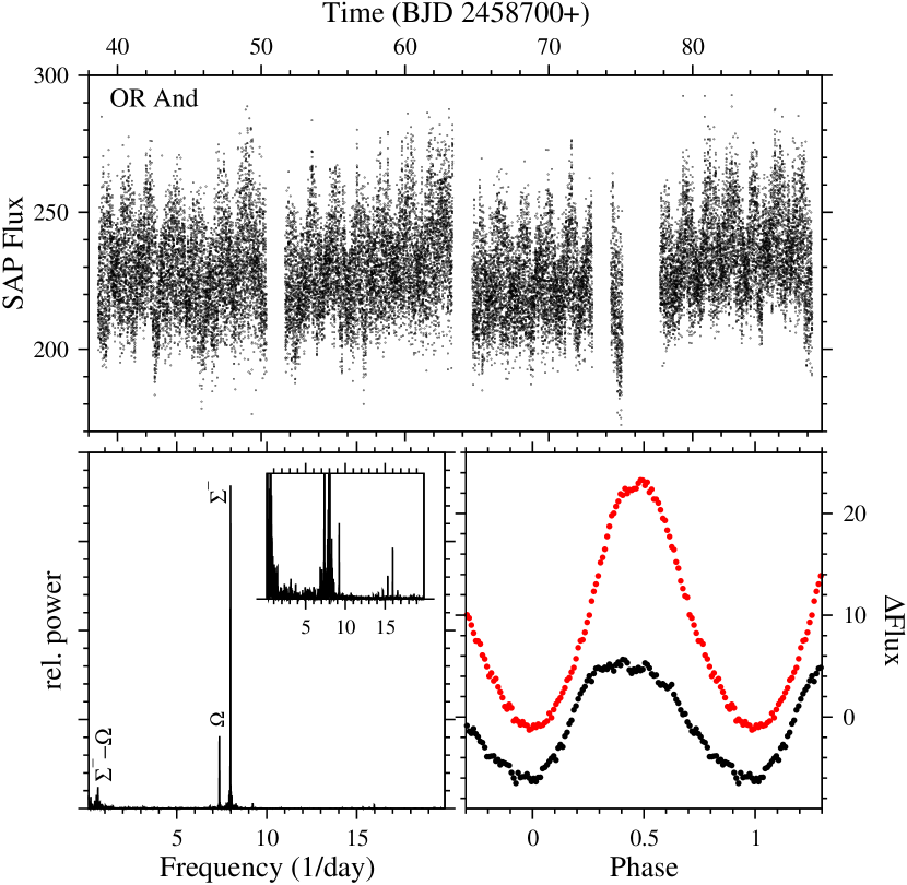
Figure 1: Light curve (top) and power spectrum (lower left) of LC#1 of OR And, and waveforms (lower right) of the orbital (black) and superhump (red) variations averaged over LC#1 and LC#2.

3.2 LS Camelopardalis

The only detailed study of LS Cam was published by Dobrzycka et al. (1998). They found radial velocity, flux and equivalent width variations in the He II $\lambda$4686 emission line with a period of $\approx$50 min which they attribute to the Alvén radius of the WD. This apparently caused RK to classify the system as an intermediate polar (IP) candidate. The TESS light curves do not contain indications for an IP nature of LS Cam. The tentative orbital period cited by Dobrzycka et al. (1998) was later revised by Thorstensen et al. (2017) to be 0.1423853(5) d.

TESS observed LS Cam in seven sectors. The data of the first and the last two sectors can be combined. Thus, five light curves are available. The subsequent frequency analysis leads to conclusions similar to those obtained by Rawat et al. (2022) based on the same TESS data (except LC#5), but addresses also some additional aspects.

All light curves exhibit a well expressed periodic modulation close to 4 days. The upper frame of Fig. 2 shows light curve LC#1. The yellow curve is the sum of a low order polynominal (to follow more gradual variations) and a sine curve fitted to the data. The obvious periodicity suggests to be the beat between the orbital and a superhump modulation. This is confirmed by the power spectra. The lower left frame of Fig. 2 contains the spectrum of LC#3. Fig. 3 provides a more detailed view. The power spectra of all light curves in a small range around the orbital frequency (left) and its first overtone (right) are displayed. Apart from the orbital signal LC#1 clearly exhibits a negative superhump together with signals at the frequencies of simple arithmetic combinations of the orbital and superhump frequencies. While in LC#1 the superhump signal is still weaker than the orbital one, it outshines the latter in all other light curves. In addition to the negative superhump, in the later light curves a positive superhump is present which leads to some complexity of the power spectra around the overtone of the orbital frequency. In LC#2 the pSH signal is weak and appears to split up into three components. In fact, a dynamical power spectrum reveals a signal at slightly different frequencies in the first three quarters of the light curve (being weaker in the second quarter) which then vanishes totally in the last quarter. The exact period of the superhumps varies slightly from one epoch to the next. The values cited in Table 3 are averages. Thus, LS Cam belongs to the growing group of CVs which exhibit positive and negative superhumps simultaneously. As expected considering the strong 4 day variability all power spectra contain a well expressed peak at the (negative) superhump – orbital beat frequency (extreme left hand edge in the lower left frame of Fig. 2), corresponding to a period of 4.004 d. On the other hand, a beat signal with the orbital period caused by the positive superhump is not seen. However in LC#3 and LC#4 (and marginally also in LC#2) the beat between the two superhumps and its first overtone appear.

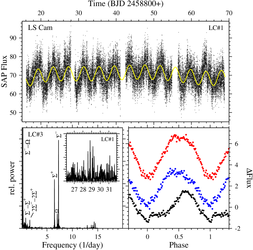
Figure 2: Top: Light curve LC#1 of LS Cam. The yellow curve is the sum of a low order polynominal (to follow more gradual variations) and a sine curve fitted to the data. Bottom left: Power spectrum of LC#3. The inset shows a part of the power spectrum of LC#1 with possible QPOs consistent with $\approx$50 min variations reported by Dobrzycka et al. (1998). Bottom right: The waveforms (average of LC#1 – LC#5 for orbit and nSH, and of LC#2 – LC#4 for pSH), referring to (from bottom to top) the orbital, pSH and nSH variations.

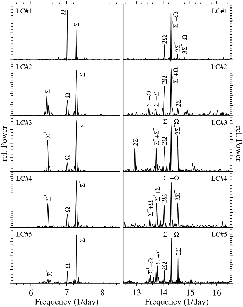
Figure 3: Power spectra of the five light curves of LS Cam in the range around the orbital frequency (left) and its first overtone (right).

The waveforms of the orbital (black), positive (blue) and negative (red) superhump variations, averaged over all light curves (but restricted to LC#2 – LC#4 for the pSH), are shown in the lower right frame of Fig. 2. The orbital waveform consists of a hump encompassing 60–70% of the orbit. The slight depression after the hump may indicated shallow eclipses in LS Cam.

Although all five TESS light curves clearly exhibit the negative superhump this is not a permanent feature of LS Cam but only developed in recent years. The upper frame of Fig. 4 contains the ASAS-SN long term light curve of the system (blue dots: $V$ band; green dots: $g$ band). The small red bars indicate the intervals covered by the TESS data. The lower left frame shows the power spectrum of the light curve. The peak at low frequencies corresponds to a synodic month and can thus be attributed to data sampling. More importantly, two closely spaced signals at 0.2503 and 0.2568 d^-1 have frequencies which are almost identical to the difference between the orbital and nSH frequencies (ranging between 0.245 and 0.255 d^-1 in LC#1 – LC#5). Thus, in spite of the much lower cadence the ASAS-SN data doubtlessly exhibit the beat between orbit and superhump which is so prominent in the TESS data. However, as the dynamical power spectrum in the lower right frame of Fig. 4 (calculated with a sliding window of 1 yr width) shows, it only started shortly before the first TESS observation.

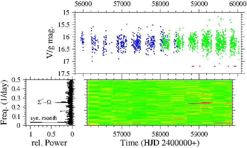
Figure 4: Top: ASAS-SN long term light curve of LS Cam. The blue and green dots refer to the $V$ and $g$ bands, respectively. The red bars beneath the light curve indicate the intervals when TESS observed LS Cam. Bottom: Power spectrum of the ASAS-SN light curve in the conventional (left) and time resolved (right) forms.

Finally, the light curves do not contain evidence for a consistent 50 min variation as reported by (Dobrzycka et al., 1998) in their spectroscopic observations. However, the power spectrum of LC#1 does have some faint peaks in the frequency range between 28.5 – 29.5 d^-1 (inset in the lower right frame of Fig. 2) which may indicated quasi-periodic oscillations (QPOs) with a period close to 50 min. But there are no similar signals in the other light curves.

3.3 NS Cancri

Identified spectroscopically as a cataclysmic variable by Szkody et al. (2004) among the stars observed in the Sloan Digital Sky Survey, NS Cnc (= SDSS J081256.85+191157.8) was found to be deeply eclipsing by Gülseçen & Esenoglu (2014). The most accurate value of 0.1600525(30) d for the orbital period was determined by Thorstensen et al. (2015). Gülseçen & Esenoglu (2014) attribute another period of 0.148159 d to a negative superhump. The ASAS-SN long term light curve (not shown) reveals that from about mid-2016 on NS Cnc steadily increased its brightness at a rate of 0.084 mag/yr. Starting from a previously constant level of $V\approx 16.1$ it has reached $g\approx 15.6$ by early 2023.

NS Cnc was observed by the Kepler satellite as part of the K2 mission during campaigns 5 and 18 with an interval of about 3 yrs between them. Additionally, TESS observed the star in three consecutive sectors after another 3 yrs. All light curves are reproduced in the left column of Fig. 5. Considering that the TESS data are noisier and therefore cannot reveal as many details as the Kepler data, the general structure of LC#1 and LC#3 is similar with the out-of-eclipse variations largely being dominated by modulations on time scales of several days and shorter variations superposed (better seen in LC#1). In contrast, LC#2 is characterize by a very clear, strict periodicity with a period of about 3 d which immediately suggests to be the beat between two other periods. The yellow curve is the best fit to the out-of-eclipse light curve of the sum of a low order polynomial (to fit slight long term variations) and a sine function with a period of 3.046 d.

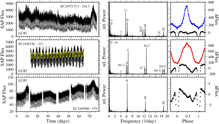
Figure 5: Left: Light curves of NS Cnc. LC#1 and LC#2 were observed by Kepler, LC#3 by TESS. Middle: Power spectra of the light curves. Right: Waveforms of the orbital variations (black), and of the positive (blue) and negative (red) superhumps.

The power spectra of all light curves (eclipses masked) is reproduced in the central column of Fig.5. Apart from the orbital signal the power spectrum of LC#1 contains a strong peak at a frequency corresponding to a period of 0.17463(3) d. It can be interpreted as being due to a positive superhump. Overtones and combinations of the orbital and superhump signal, in particular the beat frequency $\Omega-\Sigma^{+}$, are identified in the figure. The superhump does not persist over the entire duration of the light curve. Instead, it suddenly vanishes right in the middle. This is seen in Fig. 6 where the power spectrum of the original data (i.e., including the eclipses) in a small frequency range encompassing the superhump and the orbital signal is shown in the conventional form at the left, and time resolved in the right frame. A sliding window of 10 d width was used in this case to calculate the dynamical power spectrum. The superhump waveform (right column of Fig. 5) is far from sinusoidal and consists basically of a narrow hump.

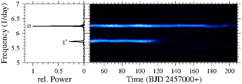
Figure 6: Power spectrum of LC#1 of NS Cnc in a narrow frequency range around the positive superhump and orbital frequency in conventional (left) and time resolved form (right).

Turning the attention now to LC#2, the power spectrum shows that the positive superhump has gone and made room for a negative one. The strongest peak in the spectrum (truncated in the Fig. 5) is caused by the beat between the superhump and the orbit. Other combinations and overtones are identified in the figure, and many more can be detected at higher frequencies up to the Nyquist frequency. The superhump period is 0.152042(6) d. In contrast to the positive superhump in LC#1 the nSH remains active over the entire duration of the light curve. The waveform is almost sinusoidal with a curious extra hump upon the maximum. It is noteworthy that its period is much longer than the 0.148159 d period seen by Gülseçen & Esenoglu (2014). The latter implies a much higher period excess as will be discussed in Sect. 4.

Finally, the power spectrum of LC#3 shows that the superhumps have vanished altogether. Only the orbital signals and its overtones remain.

The light curves also reveal an evolution of the orbital waveform of NS Cnc (black curves in the right column of Fig. 5). In all cases, out of eclipse it consists of a hump with some superposed structure. However, the phase of its maximum changes from epoch to epoch. A secondary eclipse is also seen in all light curves, although in LC#2 it causes only a slight depression on the downward slope of the orbital hump.

3.4 V425 Cassiopeiae

Our knowledge of the novalike variable V425 Cas is quite limited. Long-term observations of Wenzel (1987) revealed low states, permitting a classification as a VY Scl star. A spectroscopic period of 0.14964(36) d was reported in a short notice of Shafter & Ulrich (1982). Large amplitude variations (up to 1.5 mag) with a period of 2.65 d were seen by Kato et al. (2001) who interpret them – not without difficulties – as being due to a combination of disk instabilities and irradiation of the secondary star.

Such variations are not present in the two single sector light curves observed by TESS with an interval of 3 yr between them. LC#1 is reproduced in the upper frame of Fig. 8. The power spectra of the light curves contain considerable noise due to irregular variability on time scales longer than 0.5 d. At higher frequencies they are quite different from each other (left frame of Fig. 7). In LC#1 (black graph) two significant signals are present. One of them corresponds to a period just two standard deviations shorter than the orbital period measured by Shafter & Ulrich (1982). The revised value is listed in Table 3. The lower frequency peak ($P_{\rm pSH}=0.1654$ d) can then be interpreted being due to a positive superhump. In contrast, in LC#2 a single peak slightly above the orbital frequency ($P_{\rm nSH}=0.14509(3)$ d) appears to be due to a negative superhump. The orbital signal itself is not seen, and neither is the pSH. Thus, in the interim between the light curves V425 Cas has changed from a positive to a negative superhump regime. The orbital (black; LC#1), pSH (blue; LC#1) and nSH (red; LC#2) waveforms are shown in the right frame of the figure. They are all very nearly sinusoidal.

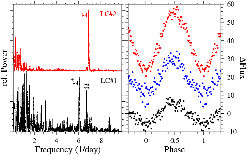
Figure 7: Left: Power spectra of LC#1 and LC#2 of V425 Cas. Right: Waveforms of the orbital (black, LC#1), pSH (blue; LC#1) and nSH (red; LC#2) variations.

While dynamical power spectra reveal that the negative superhump is persistent over the entire length of LC#2, this is not the case for the pSH in LC#1, as is shown in the lower frames of Fig. 8 which contains a small part of the power spectrum in the range close to the orbital and superhump frequencies in the conventional form on the left, and in time resolved form on the right. It reveals that the superhump is completely absent in the first half of the light curve and appears only after the gap in the middle of the TESS observations.

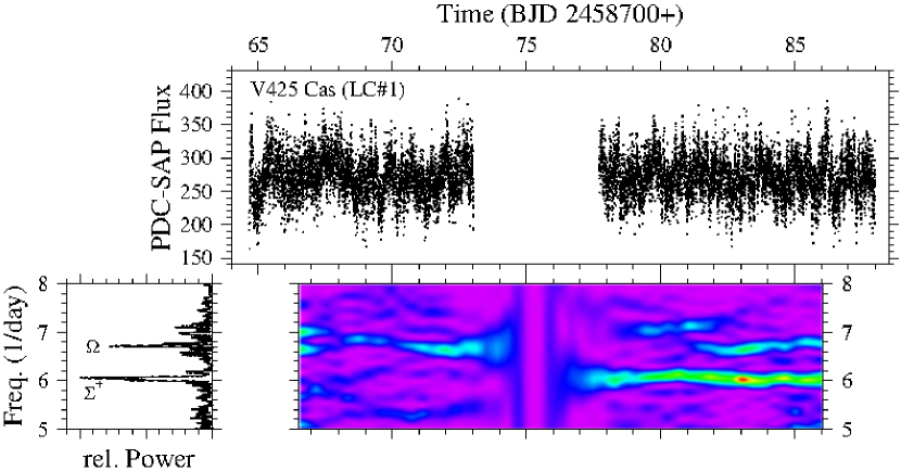
Figure 8: Top: Light curve LC#1 of V425 Cas. Bottom: Power spectrum of the light curve in a small range around the orbital and pSH frequencies in the conventional (left) and dynamical form (right).

In order to avoid possible misinterpretations of a marginally significant signal at 126.6 d^-1 in LC#1 (not shown), which may at first glance point at an intermediate polar nature of V425 Cas, I note that a close inspection reveals it to be not persistent but caused by an isolated event in the light curve.

3.5 V1024 Cep

V1024 Cep (originally named HS 0455+08315) was discovered as an eclipsing cataclysmic variables by Gänsicke et al. (2002). They suspected it to be a SW Sex star. This classification was confirmed by Rodríguez-Gil et al. (2007a) who also measured a precise orbital period. Shears et al. (2016) detected deep low states in the long-term light curve of V1024 Cep. It is thus also a VY Scl star.

TESS observed V1024 Cep multiple times. The data can be combined into five light curves, four of which consist of two sector observations and one comprises only a single sector. Light curves LC#1, LC#4 and LC#5 are reproduced in the left column of Fig. 9. The yellow curve layed over the LC#5 light curve is the sum of a low order polynominal (to follow more gradual variations) and a sine curve fitted to the out-of-eclipse data. The light curves are obviously of quite different character. Their power spectra are shown in the central column of the figure. Just as the spectrum of LC#1, those of LC#2 and LC#3 (not shown), all taken before 2022, contain only signals at the orbital frequency and overtones. This changed in 2022 (LC#4 and LC#5), when a negative superhump developed and grew stronger over time. In the spectrum of LC#5 many combinations of the orbital and superhump frequencies can be identified (also at higher frequencies beyond the limits of the figure). While variations on the beat period between orbit and superhump start to develop in the latter part of LC#4 (but are not clearly identified in the power spectrum), they are prominent in LC#5 and appear to increase in amplitude over time. The superhump period is 0.142990(9) d in LC#5 (and slightly longer in LC#4).

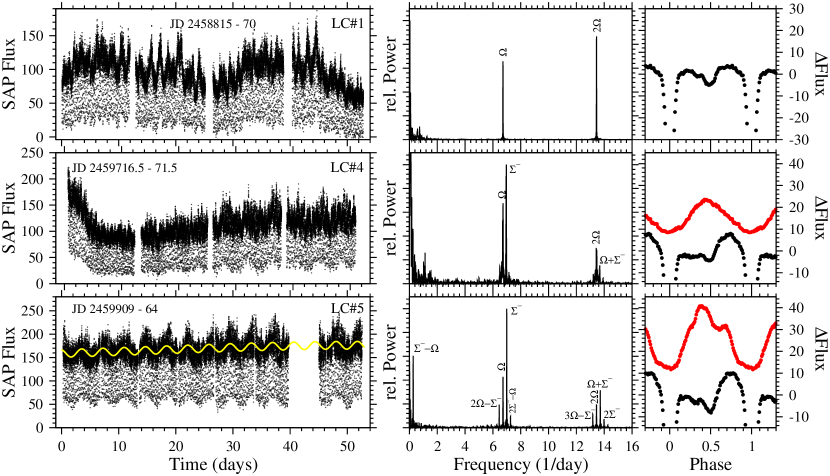
Figure 9: Left: Three of the five available TESS list curves of V1024 Cep. The yellow curve in the lower frame is the sum of a low order polynominal (to follow more gradual variations) and a sine curve fitted to the out-of-eclipse data.Middle: Power spectra of the light curves. Right: Waveforms of the orbital (black), and superhump (red) variations.

Orbital and superhump waveforms are shown in black and red, respectively, in the right column of Fig. 9. The orbital waveform contains a clear secondary eclipse. Before the superhump developped, only a small hump before the primary eclipse is seen. The waveform is quite stable in the three light curves LC#1 – LC#3. As a curious feature I note the small dip at phase 0.34 which is also seen in LC#5. During the presence of the superhump the orbital waveform changes significantly in the sense that the hump grew much stronger. The superhump waveform also underwent an evolution. While it is still almost sinusoidal in LC#4, it is much more structured and has a secondary maximum in LC#5.

3.6 DN Geminorum

The only available time resolved photometric study of the 1912 nova DN Gem revealed a period of 0.126744(5) d (Retter et al., 1996) which the authors consider to be orbital, although they also discuss (but discart) alternatives, i.e, the WD spin period in an intermediate polar scenario or a superhump period. The orbital nature of the variations was later confirmed spectroscopically by Peters & Thorstensen (2006)

Three TESS light curves of DN Gem are available. The first is separated from the second by almost 2 yrs, but only a single sector separates the second from the third light curve. As an example LC#2 is shown in the upper frame of Fig. 10. Just as the others it contains only smooth variations on time scales of many days. The power spectra in a narrow range around the orbital frequency are shown in three of the lower frames of the figure. LC#1 and LC#2 (and rather weakly also LC#3) show a clear signal corresponding to a mean period of 0.12783(8) d, only slightly – but significantly, considering the error margins – different from the orbital period of Retter et al. (1996), but within the limits of the spectroscopic period of Peters & Thorstensen (2006). I take this as the true value. In all light curves, the orbital waveform is very nearly sinusoidal (black dots in the lower right frame of the figure).

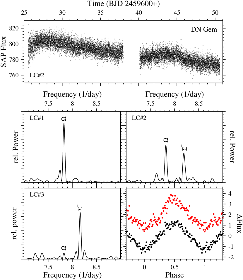
Figure 10: Light curve LC#2 of DN Gem (top) together with the power spectra of the three light curves of DN Gem in a narrow range around the orbital and the nSH frequencies. The lower right frame contains the orbital (black) and superhump (red) waveforms.

No other significant signal is present in the power spectrum of LC#1. But both other light curves, closely spaced in time, contain a signal at a somewhat higher frequency. While its strength rivals with that of the orbital signal in LC#2 it is much stronger in LC#3. Obviously, between the first and the later observing epochs a negative superhump has developed in DN Gem. Its period and the period excess are listed in Table 3, and it average waveform is shown in lower right frame of Fig. 10 as red dots. Note that details such as the small intermediate maximum at phase 0.15 are present in the waveforms of both, LC#2 and LC#3, and may therefore be real and persistent structures.

3.7 V1084 Herculis

V1084 Her is known as a negative superhump system. Since it was not included in the study of TESS light curves of superhumpers in Paper II its properties are characterized here. First detected by Mickaelian et al. (2002) the nSHs were further studied by Patterson et al. (2002) who also measured the orbital period of 0.120560(14) d. On shorter time scales Mickaelian et al. (2002) reported variation of the order of 15 min. Similarly, Patterson et al. (2002) mention QPOs near 1000 s. Citing a more specitic number, Rodríguez-Gil et al. (2009) claim the presence of a polarimetric period of 19.38(39) min and emission-line flaring on twice this period which they relate to the rotation of the WD. This intermediate polar hypothesis was, however, refuted by Worpel et al. (2020) who did not see corresponding variations in X-rays and concluded that V1084 Her is a non-magnetic CV.

The two available single sector TESS light curves confirm the presence of superhumps. The wiggles seen in LC#1 (upper frame of Fig. 11) give rise to a low frequency signal corresponding to a period of 3.86(4) d in the power spectrum (left frame in the central row of the figure) which can readily be interpreted as the beat between the faint orbital signal which is barely resolved from the strong superhump peak in the figure (but see the inset). In LC#1 the superhump waveform is approximately sinusoidal (right middle frame; red dots) while the lower amplitude and noisier orbital waveform (black) seems to have some more structure. Some differences are seen in LC#2. The orbital signal cannot clearly be detected in the power spectrum which is reproduced on an expanded vertical scale in the lower left frame of Fig. 11. But its first overtone is clearly present, as is the overtone of the SH signal. Correspondingly, the orbital waveform (lower right frame, in black) is now double humped. The SH waveform (red) also changed considerably, having a flat minimum encompassing about 40% of the cycle.

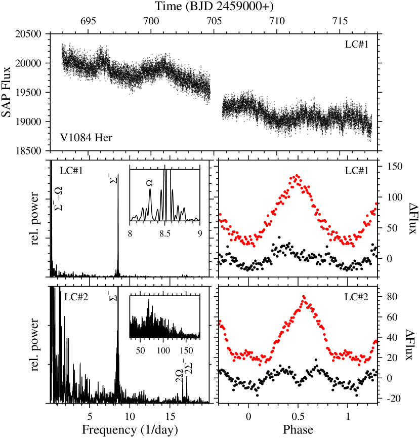
Figure 11: Top: Light curve LC#1 of V1084 Her. Middle left: Power spectrum of LC#1, dominated by a nSH signal and the beat signal between orbit and nSH. The expanded scale used in the inset permits a better identification of the orbital signal. Middle right: Waveforms of the orbital (black) and superhump (red) variations in LC#1. Lower left: Power spectrum of LC#2 on an expanded vertical scale permitting the clear identification of the overtones of the orbital and superhump signals. In inset shows a broad range of QPO signals. Lower right: Waveforms of orbital (black) and superhump (red) variations in LC#2.

At higher frequencies, the power spectra show somewhat enhanced power in a broad range between 50 and 130 d^-1 (more so in LC#2 than in LC#1; inset in the lower left frame of Fig. 11), but they do not indicate a strong preference for variations to occur on the times scales mentioned by Mickaelian et al. (2002) and Patterson et al. (2002).

3.8 CP Lacertae

The old nova (1935) CP Lac did not attract much attention in the past. In a limited amount of high time resolution photometry Rodríguez-Gil & Torres (2005) suspect the presence of a 0.127 d periodicity together with a slight dip in the phase folded light curve and wonder whether it may be due to an eclipse or not. This photometric period is, however, not orbital since radial velocity measurements of Peters & Thorstensen (2006) yielded a period of 0.145143(1) d.

TESS observations in four sectors can be combined into two light curves separated in time by about 2 yrs. No strong variations on time scales of days are present. The power spectrum of LC#1 (left frame of Fig. 12, in black) contains no signal but the orbital one. The 0.127 d period seen by Rodríguez-Gil & Torres (2005) can be explained as a 1/day alias of the true orbital period, introduced by the temporal distribution of their observations. However, another period of 62.7(3) min seen by them (beyond the limits of the figure) is definitely not present in the TESS data.

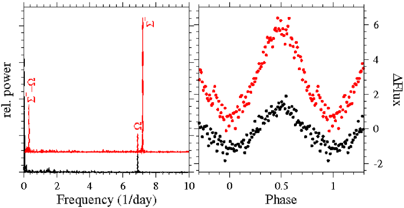
Figure 12: Left: Power spectra of LC#1 (black) and LC#2 (red) of CP Lac. Right: Orbital (black; average of LC#1 and LC#2) and superhump (red; LC#2) waveforms of CP Lac.

This is also true for LC#2, the power spectrum of which otherwise contains a strong peak at a frequency somewhat higher than the orbital frequency (red graph in the left frame of Fig. 12). This is undoubtedly due to a negative superhump. A clear signal is also present at the beat frequency between the orbit and the superhump. The SH waveform (red dots in the right frame of Fig. 12) is very nearly sinusoidal. The same is true for the orbital waveform (black dots) which does not contain any indication of the eclipse suspected by Rodríguez-Gil & Torres (2005).

3.9 DK Lacertae

Only little time resolved photometry of DK Lac (Nova Lac 1950) has been published. Katysheva & Shugarov (2008) found a possible period of 0.1296 d in 2003 which is, however, rejected to be orbital by Schaefer (2022). Also, variations on time scale of 0.11 – 0.13 d appear to be present in 2004 (Katysheva & Shugarov, 2008). On longer time scales, the system exhibited at least one episode of a VY Scl-like low state.

Data from two TESS sectors can be combined into a single light curve. Three years later TESS observed the system again in one sector. LC#1 is displayed in the upper frame of Fig. 13. It does not contain strong variations above the noise level. However, the power spectrum (lower left frame of the figure) contains, apart from some low frequency noise, a pair of signals which suggest to be due to orbital and superhump variations. The corresponding periods are $P_{1}=0.12963(5)$ d and $P_{2}=0.11644(4)$ d. $P_{1}$ is very close to the period seen by Katysheva & Shugarov (2008). If this is the orbital period, $P_{2}$ must be considered a negative superhump, leading to an uncomfortable high period excess of $\epsilon=-0.103$. The alternative, $P_{2}$ being orbital and $P_{1}$ the period of a positive superhump, gives $\epsilon=0.113$, still quite high for the period (see Fig. 31), but not to such an extend. Therefore, I tentatively identify DK Lac as a positive superhump system. The quite noisy superhump waveform (blue dots in the lower left frame of the figure) cannot be distinguished from a simple sine curve. The same is true for the orbital waveform (black dots). The power spectrum of LC#2 does not exhibit the pair of superhump and orbital signals. However, an otherwise inconspicuous (in view of the surrounding noise) peak is present at the orbital frequency.

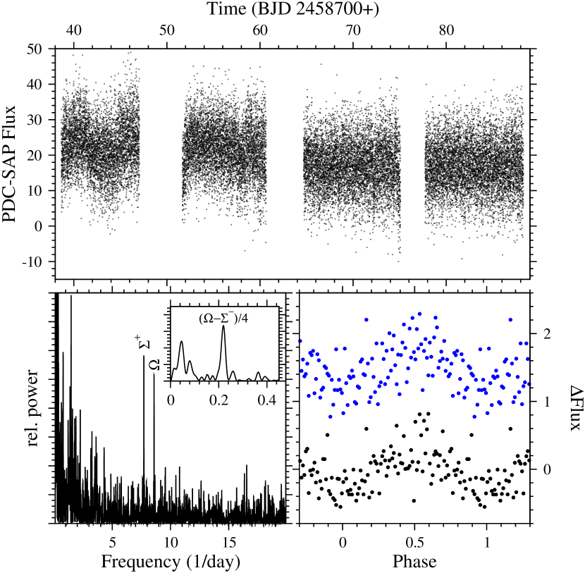
Figure 13: Light curve LC#1 (top), power spectrum (lower left) and waveforms (lower right) of the orbital (back) and superhump (blue) variations of DK Lac.

Finally, it is worth mentioning that the power spectrum of LC#1 contains a strong low frequency peak corresponding to 4.56(3) d (inset in the lower left frame of Fig. 13). Within the formal $1\sigma$ error limits this is equal to 4 times the beat between the orbital and superhump periods. Thus, DK Lac appears to join the select group of superhumping CVs with a modulation on an integral multiple or fraction of the accretion disk precession period (see Sect. 4).

3.10 KQ Monocerotis

KQ Mon was originally classified as a CV by Bond (1979). While the ultraviolet spectral properties of the star have been reasonably well studied (Sion & Guinan, 1982; Wolfe et al., 2013), time resolved photometry of the system is completely missing in the literature. Based on optical spectroscopy in two nights Schmidtobreick et al. (2005) determined an orbital period of 3.08(4) h (= 0.128(2) d), but cannot exclude several alias periods.

When I had already analyzed the single sector TESS light curve of KQ Mon Stefanov & Stevanov (2023) published their study of the same data. I therefore restrict myself here to summarize the results and to put forward an additional argument. The power spectrum contains two signals corresponding to periods of $P_{1}=0.13450(3)$ d and $P_{2}=0.12895(1)$ d together with a signal at the beat frequency. Thus, it is obvious that the light curve contains the orbital and a superhump signal, together with the disk precession period. But which of $P_{1}$ and $P_{2}$ is orbital and which is due to the SH? $P_{2}$ lies within the $1\sigma$ error margin of the spectroscopic orbital period of Schmidtobreick et al. (2005), but the same is true for $P_{1}$, if an alias period at 0.134(2) d is taken. Stefanov & Stevanov (2023) argue in favour of $P_{1}$ being orbital and $P_{2}$ being due to a negative superhump. I agree with this interpretation and add as an additional argument a comparison between the observed period excess $\epsilon_{\rm obs}$ and its expected value $\epsilon_{\rm SS}$ from the Stolz-Schoembs relation, i.e., the relation between the superhump period and the period excess (Sect. 4). We then have $\epsilon_{\rm obs}=-0.041$ versus $\epsilon_{\rm SS}=-0.36$. The alternative case of $P_{2}$ being the orbital and $P_{1}$ the (positive) superhump period yields $\epsilon_{\rm obs}=0.043$ versus $\epsilon_{\rm SS}=0.065$. Thus, the nSH hypothesis is in better agreement with the expectations.

3.11 LZ Muscae

Practically nothing is known about the quiescent state of Nova Muscae 1998 = LZ Mus. Even the (not well documented) orbital period quoted by Retter et al. (1998) in a short IAU Circular as $P_{\rm RLG}=0.16930(15)$ d (or an alias at 0.20390(25) d) may not be trustworthy because it refers to variations observed soon after outburst during the nova transition phase when the system was far from its quiescent state. RK quote the first of these values as the orbital period of LZ Mus but mark it as uncertain.

TESS observed the star in two consecutive sectors. Thus, the data can be combined into a single light curve which, however, is quite noisy due to the faintness of LZ Mus (upper frame of Fig. 14). Correspondingly, the power spectrum (lower left frame of the figure) is also noisy, but it contains a clear signal at $P_{1}=0.16348(5)$ d, somewhat shorter than $P_{\rm RLG}$ It is accompanied by a less prominent signal at a slightly shorter period of $P_{2}=0.15097(7)$ d. How to interpret the different periods? The prominence of the $P_{1}$ signal suggests that this is the orbital period. This assumption is strengthened by what appears to be a shallow eclipse suggested by the phase folded light curve shown in the lower right frame of the figure as black dots. However, in view of the noise in the waveform, this requires confirmation. Assuming $P_{1}=P_{\rm orb}$ one might speculate that $P_{\rm RLG}$ is due to a positive superhump in the newly formed accretion disk just after the nova outburst. Although at $\epsilon=0.036$ the period excess would then be much smaller than 0.082 as predicted by the Stolz-Schoembs relation (Sect. 4), the scatter around that relation (Fig. 31) would still encompass the low period excess.

The significance of the $P_{2}$ signal may be doubted in view of its low strength. Considering it to be real and interpreting it as being caused by a negative superhump, the situation is reversed: The period excess of $-0.077$ is much larger than predicted by the Stolz-Schoembs relation ($-0.040$). However, other systems with higher nSH credentials have a similarly excessive period excess; an issue which will be discussed in Sect. 4. Therefore, I tentatively assume LZ Mus to exhibit nSHs. Their waveform (red dots in the lower right frame of Fig. 14) is very noisy and can only be distinguished from noise after binning the data in larger phase bins. I emphasize, however, that the identification of $P_{RLG}$ and $P_{2}$ as positive and negative superhump periods, respectively, is only tentative.

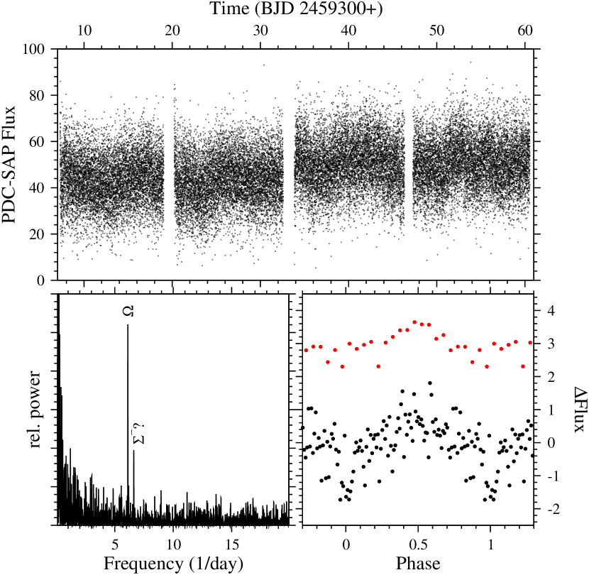
Figure 14: Light curve (top), power spectrum (lower left) and waveforms (lower right) of the orbital (back) and superhump variations (red) of LZ Mus.

3.12 FY Persei

No detailed studies of FY Per resolving short time scales are available in the literature. The two single sector TESS light curves, separated in time by 3 yrs (displayed in the top frames of Fig. 15 on the same flux scale) contain well expressed outburst-like events. This is consistent with the long-term behaviour of the system investigated in some detail by Honeycutt (2001) (see also Honeycutt & Kafka, 2004) who observed the “common occurrence of 0.6 mag oscillations with a characteristic interval of 20–25 days”. This aspect of FY Per will be analyzed in a separate paper. Honeycutt (2001) also identified the system as a VY Scl star.

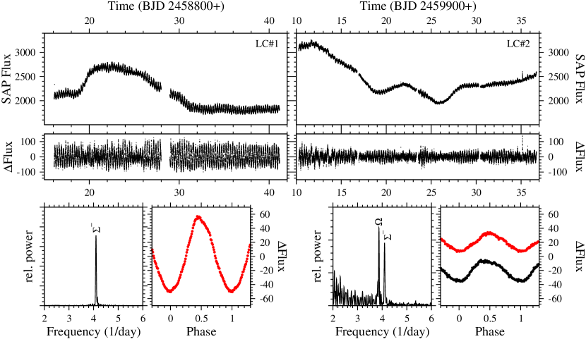
Figure 15: Top: Light curves of FY Per drawn on the same flux scale. Middle: Light curves after subtraction of variations on time scales longer than 2 d, dominated by negative superhumps in LC#1 and the interplay between superhump and orbital modulations in LC#2. Bottom: Power spectra (left), and superhump (red) and orbital (black) waveforms (right) for both light curves.

The most impressive features of the TESS light curves are, however, strong periodic modulations on the time scale of hours, easily visible to the unaided eye. They are persistent over the entire duration of the light curves and have a much higher amplitude in LC#1 than in LC#2, as is obvious from the second row of frames in Fig. 15 where the residuals after subtracting variations on time scales longer than two days are plotted on the same flux scale. Not surprisingly, these variations cause strong signals in the power spectra displayed in the lower frames of the figure.

In the power spectrum of LC#1 only one peak appears (together with a very weak first overtone). It corresponds to a period of 0.24400(3) d. Trusting that the spectroscopic period of 0.2584(3) reported by Thorstensen et al. (2017) is indeed orbital, I conclude that FY Per exhibits negative superhumps. The SH waveform (see lower frames of Fig. 15) is nearly sinusoidal with a slightly skewed maximum. The orbital period is not detected in the power spectrum. However, the strongest low frequency peak (after removing the outburst-like structure) has a frequency different by just 1.3 times the formal $1\sigma$ error margin of the beat period calculated from the orbital and SH frequencies. It thus most probably reflects the precession period of the accretion disk.

In contrast to LC#1, the power spectrum of LC#2 contains two clear peaks. One is only slightly offset from the superhump frequency observed in LC#1, corresponding to a period of 0.24380(8) d and can thus considered to be due to the same phenomenon. The lower frequency peak corresponds to a period of 0.25837(7) d. This is within the error margin of the orbital period measured by Thorstensen et al. (2017). The orbital and superhump waveforms are of almost equal amplitude which is, however, much smaller than the superhump waveform in LC#1. Even so, a close inspection reveals that the shape of the superhump remained remarkably stable: Just after maximum the same deviations from a sinusoid can be detected in both waveforms.

As can be seen in the left central frame of Fig. 15 the amplitude of the superhumps remains roughly constant. Only during two small time intervals close to BJD 2458819.5 and 2458821 they vanish and make room for incoherent variability. A few days later (BJD 2458825) their amplitude decreases significantly for just over one day. It is remarkable, however, that the outburst-like event has apparently no bearing on the behaviour of the superhumps. This suggests that the light source responsible for the brightening is independent of the superhump light source. The same is true for LC#2 (right central frame of the figure), but in this case the amplitude of the variations varies significantly over time. This can be explained by the interplay between the orbital and superhump modulations. Indeed, an analysis of the rms-scatter of the residual light curve in bins of 0.5 d shows a clear periodicity of 4.35 d, compatible with the beat period between orbit and superhump.

3.13 LX Serpentis

LX Ser, also known as Stepanyan’s star, is a deeply eclipsing novalike variable. The orbital period of 0.158432491(2) d has been steadily refined by many authors over the years and was last updated by Li et al. (2017). Liller (1980) reported low states in the long term light curves suggesting a VY Scl nature for LX Ser. No other periodic brightness variations of the star have been reported.

LX Ser is a negative superhumper, but the superhumps are not permanent. The first of two single sector TESS light curve is shown in the upper frame of Fig. 16. It contains irregular and quite rapid ($<$1 d) out-of-eclipse variation superposed upon a clear periodic modulation. A least squares sine fit (yellow curve) returns a period of 3.54 d. The power spectrum has a low frequency peak corresponding to the same period within the formal error limits. Otherwise, the low frequency range contains many peaks which I attribute to irregular variations in the light curve. However, at not so low frequencies (second frame of Fig. 16; the eclipses were masked before calculating the power spectrum) some peaks stand out. I interpret a signal corresponding to a period of $P_{1}=0.15177(8)$ d as being due to a negative superhump. Its beat with the orbital period is compatible with the 3.5 d supraorbital period. This interpretation is reinforced by other signals which can be identified as simple arithmetic combinations of the SH and orbital frequencies. Others are weakly present beyond the limits of the figure. The somewhat structured superhump waveform is reproduced as red dots in the lower left frame of Fig. 16 together with the orbital waveform (in black). Away from the primary eclipse the latter consists of an asymmetrical hump, interrupted by a secondary eclipse. This shape explains why the orbital period itself only appears weakly in the (eclipses masked) power spectrum.

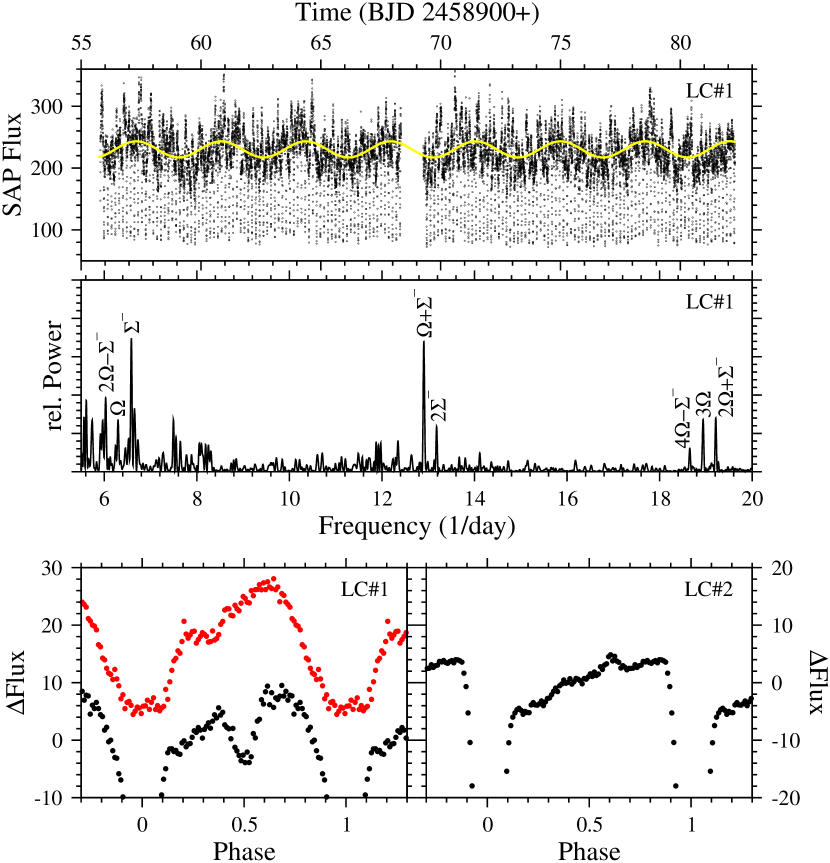
Figure 16: Top: Light curve LC#1 of LX Ser. The yellow curve is a least squares sine fit to the out-of-eclipse flux. Middle: Power spectrum of LC#1. Bottom: Waveforms of orbital (black) and superhump (red) variations in LC#1 (left) and LC#2 (right).

The power spectrum of LC#2 (not shown), observed 2 yrs later, is very different. Apart from low frequency noise it only contains signals at the orbital frequency and its overtones. Thus, the superhump has subsided. Moreover, the orbital waveform (lower right frame of Fig. 16) has also changed a lot. It consists of a single asymmetric hump, the secondary eclipse having disappeared. The long term ASAS-SN light curve shows that the average magnitude of LX Ser during the two TESS observing epochs was the same. The complete disappearance of the secondary eclipse is therefore puzzling.

3.14 EI Ursae Majoris

EI UMa is a well established intermediate polar. The spectroscopic orbital period of 0.26811(33) d (Thorstensen, 1986) places it among the longer period CVs. In optical photometric observations Kozhevnikov (2010) measured a WD spin period of 769.83(10) sec. This author also gives a detailed account of the previous optical and X-ray observational history of the star, to which the reader is referred for further references.

Light curves from two TESS sectors are available, separated by two years. They are displayed in the upper frames of Fig. 17. Both of them show episodes of strong outbursts of short duration ($<$0.5 d) in quick succession. Those of LC#1 have already been discussed by Scaringi et al. (2022a). Similar event have been observed in several other intermediate polars and were explained in terms of a magnetic gating model (Hameury et al., 2022; Littlefield et al., 2022) or invoking localized thermonuclear bursts on the white dwarf (Scaringi et al., 2022a, b). More outbursts of similar nature can be identified in the long term ASAS-SN light curve of EI UMa. They will not be discussed in more detail here and have been purged from the light curves before further analysis. However, it is noteworthy that in both light curves they are superposed upon a temporary brightening of EI UMa which lasts for about 10 days. During these epochs the light curves become noticably more rugged (better seen in Fig. 18).

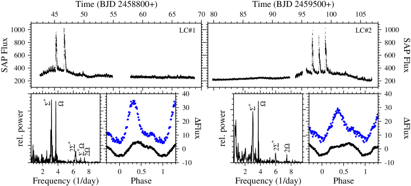
Figure 17: Top: Light curves of EI UMa drawn on the same flux scale. Bottom: Power spectra (left), and superhump (blue) and orbital (black) waveforms (right) for both light curves.

Concerning the IP type variations of EI UMa, and considering that this is not the main topic of this study, I restrict myself here to state that the power spectrum only contains weak signals at the WD spin period. No trace of an orbital sideband signal can be detected. The period is entirely consistent with the value measured by Kozhevnikov (2010).

While the IP nature of EI UMa is well known the TESS light curves for the first time reveal the system also to be a positive superhumper. This was alread briefly mentioned by Scaringi et al. (2022a) but is discussed in more detail here. In the lower frames of Fig. 17 the low frequency parts of the power spectra are displayed. Both contain two dominant signals. One is due to the orbital motion of EI UMa and yields a period slightly longer but within the error margin of the spectroscopic period of Thorstensen (1986). The second one is somewhat structured in both light curves. This complicates the measurement of an exact period. I interpret it as being due to a positive superhump with a slightly varying period.

The time dependent behaviour of the orbital and superhump signals can be studied in the dynamical power spectra in the second and third right hand frames of Fig. 18. For comparison, on the left side the conventional power spectra in a narrow frequency range around the signals are reproduced. On top and at the bottom the light curves are drawn, where the rapid outbursts (see above) were removed. In both light curves the orbital signal vanishes during the brightenings upon which the outbursts are superposed. In LC#1 the superhump signal is strong during the brightening ($P=0.317$ d), then disappears and reappears during what may be a small secondary brightening ($P=0.323$ d). During the second half of the light curve it is missing altogether. In LC#2 the superhump is faintly present from the start, grows in strength as the brightness of EI UMa gradually increases ($P=0.354$ d), and becomes strong, but at a slighly higher frequency ($P=0.336$) d, during the fully developed brightening, only to vanish when EI UMa returns to its normal brightness. The changing SH periods imply a range of period excesses between 0.181 and 0.319. The superhump waveform changes somewhat, but its general structure remains the same (lower frames of Fig. 17; in blue). In contrast, the orbital waveform (black) evolves significantly between LC#1 and LC#2.

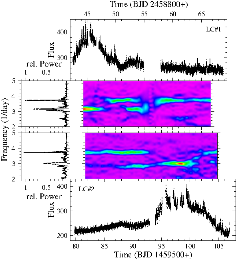
Figure 18: Light curves LC#1 and LC#2 of EI UMa and their power spectra. The right upper and lower frames show the light curves from which the rapid ($<$0.5 d) outbursts were removed. The left frames contain the respective power spectra in a small interval around the orbital and superhump frequencies. The remaining frames show the time resolved power spectra in the same frequency range and aligned in time with the light curves.

3.15 LN Ursae Majoris

While the long-term variations of LN UMa have been reasonable well studied and revealed it to be a novalike variable of VY Scl type (Hillwig et al., 1998; Honeycutt & Kafka, 2004), the only attempt to find regular variations in time resolved light curves was performed by Papadaki et al. (2009) and met no success. An orbital period of 0.169 d has been measured spectroscopically by Ringwald (1993). This is a 1/day alias of another period of 0.1444(1) d, measured by Hillwig et al. (1998) and which the TESS data confirm to be correct (see below). Just as many other NLs with orbital periods close to the upper rim of the CV period gap LN UMa is also a SW Sex star (Rodríguez-Gil et al., 2007b).

TESS observed LN UMa in six sectors. Some of the data can be combined which leaves us with four light curves. They are shown in Fig. 19 revealing that their character can change a lot over time. I draw particular attention to LC#4 which is dominated by a brightening with an amplitude of $\approx$0.55 mag, preceded by what appears to be the decline from a previous brightening. Similar events are also observed in the ASAS-SN long term light curve of LN UMa. Other systems of the RK sample mentioned in the Introduction show much the same behaviour which will be investigated in a separate paper.

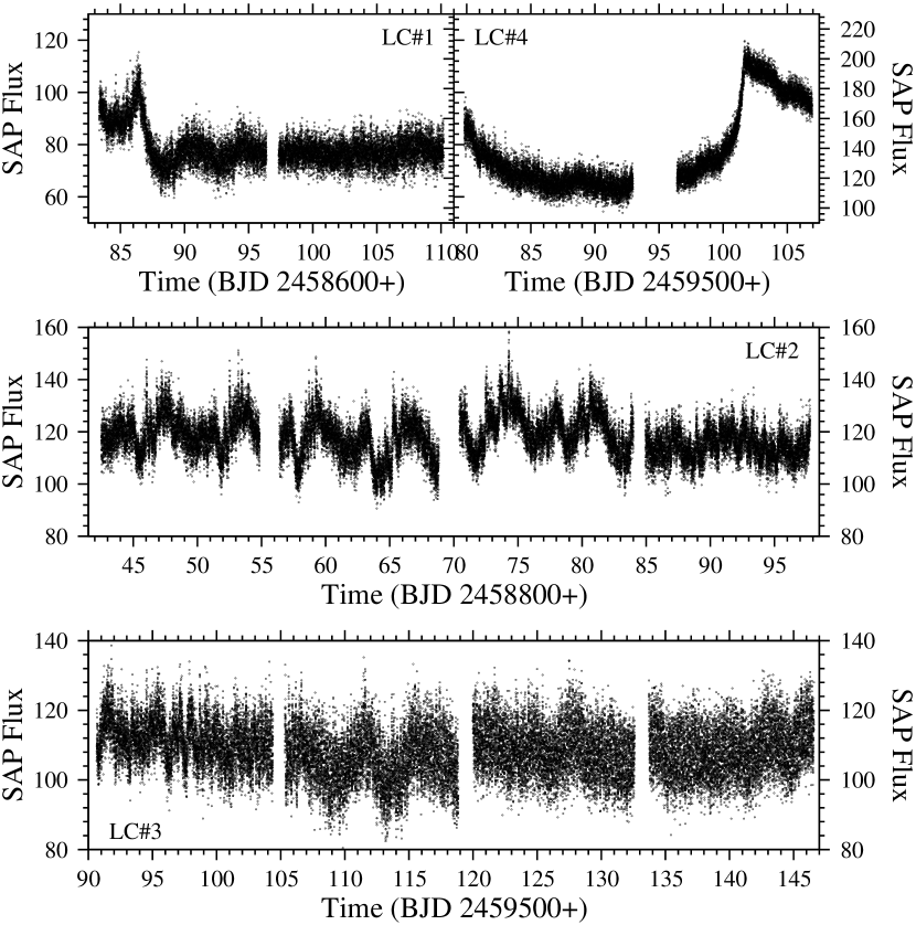
Figure 19: The four TESS light curves of LN UMa. Note that the time scale is the same but the flux scale has been adapted to the individual light curve.

The power spectra of the four light curves are not all alike. Overall they indicate the presence of orbital variations and of a negative superhump. In order to understand the differences between the individual light curves, Fig. 20 shows on the left their conventional power spectra in the relevant frequency range, and on the right the corresponding time resolved spectra. In LC#1 only a weak orbital signal is seen apart from random variations. It is not deteced in LC#2 and has made room for a much stronger negative superhump. LC#3 also does not contain the orbital signal, and the superhumps are even more developed and increase their strength over time. Finally, in LC#4 the orbital signal returns and gains in strength towards the end of the light curve. The superhump is now much weaker and appears to fade away. The superhump period evolves from 0.13797(2) d (LC#2) over 0.1383387(5) d (LC#3) to 0.13754(8) d (LC#4). The average period excess is thus $\epsilon=-0.047$. The values listed in Table 3 refer to LC#3 where the superhump is strongest. The orbital variations are most strongly seen in LC#4 where the period is measured to be 0.14471(4) d, close to the value quoted by Hillwig et al. (1998). The orbital (black) and superhump (red) waveforms constructed from LC#4 and LC#3, respectively, are displayed in the left frame of Fig. 21. The other light curves yield waveforms similar in shape, but noisier. Both consist of a single slightly asymmetric hump.

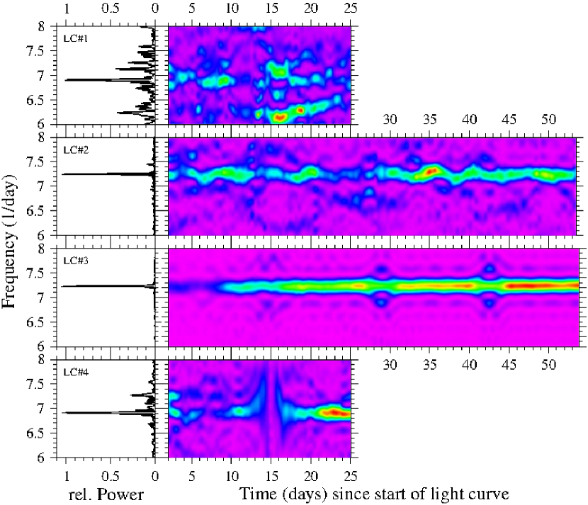
Figure 20: Power spectra of the four light curves of LN UMa in a narrow range around the orbital and superhump frequencies in the conventional (left) and the time resolved form (right).

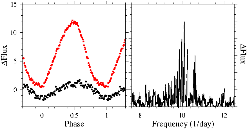
Figure 21: Left: Orbital (black) and superhump (red) waveforms constructed from LC#4 and LC#3, respectively, of LN UMa. Right: Part of the power spectrum of LC#4 of LN UMa, containing long period QPOs.

Finally, I draw attention to a concentration of peaks in the power spectrum of LC#4 in the frequency range 9–11 d^-1 (see right frame of Fig. 21). This phenomenon, also seen in other systems, will briefly be discussed in Sect. 4.

3.16 CN Velorum

+

Not many details about the quiescent properties of the 1905 classical nova CN Vel have been published. Tappert et al. (2013) measured a spectroscopic orbital period of 0.220(3) d.

CN Vel has a much brighter neighbour, only 22.6 arcsec away, TYC 8619-935-1. The magnitude difference is 3.7 mag Gaia Collaboration (2020). Considering the coarse spatial resolution of the TESS images it is quite possible that the single sector TESS light curve of CN Vel is heavily contaminated with light from this neighbour. However, TYC 8619-935-1 in not known to be variable. Therefore, the presence of variations similarly found in other CVs but not typically seen in other variable stars inspires some confidence that at least these modulations can really be attributed to CN Vel.

The light curve is shown in the left frame of Fig. 22, while its conventional power spectrum is reproduced together with its time resolved counterpart in Fig. 23. In the latter, power is shown on a square root scale in order to better visualize fainter structures. It contains some strong but enigmatic spectral lines which are identified in the left frame of the figure and are listed in Table 4 where their frequencies and periods are given. All signals are persistent over the entire duration of the light curve. Only two lines can be readily interpreted. $1/F_{6}$ lies only marginally beyond the formal error limits of the spectroscopic period of Tappert et al. (2013) and is therefore identified as being due to orbital modulations. The slightly stronger signal $F_{5}$ must then be considered as caused by a positive superhump. The noisy waveforms of both, the SH modulations (blue) and orbital variations (black), are shown in the right frame of Fig. 22 and are nearly sinusoidal.

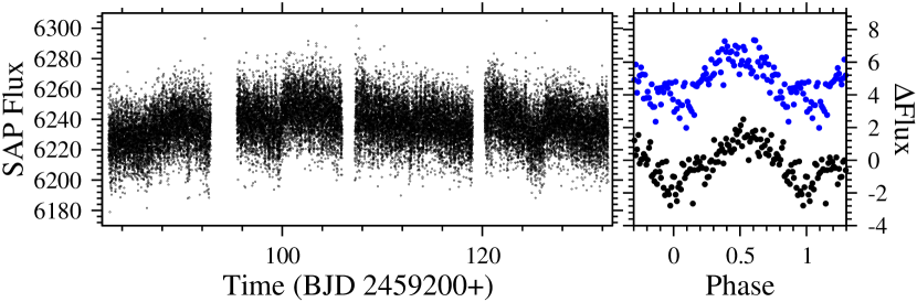
Figure 22: Left: Light curve of CN Vel, probably heavily contaminated by the brighter neighbouring star TYC 8619-935-1. Right: Orbital (black) and superhump (blue) waveforms.

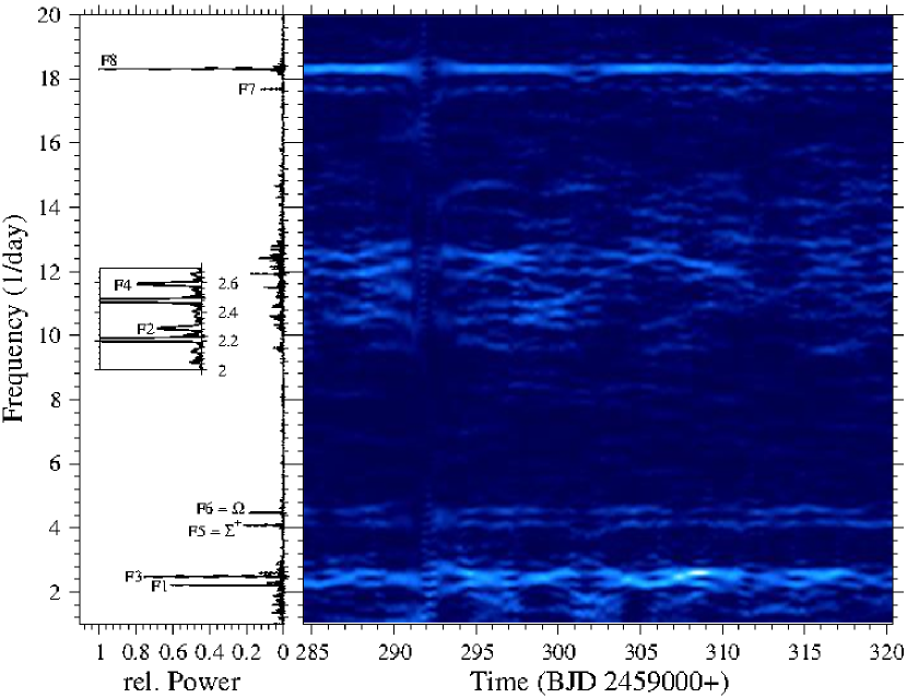
Figure 23: Left: Conventional power spectrum of the light curve of CN Vel. Spectral lines considered significant and persistent over time are identified. The inset contains a small section of the power spectrum with signals which are not well resolved in the main frame. Right: Time resolved power spectrum of the light curve. Power is scaled by its square root in order to better visalize fainter structures.

Table 4: Periodic signals identified in the power spectrum of CN Vel. Column 1: label as used in Fig. 23; column 2: frequency of the signal in 1/day; column 3: Period in days.

Feature	Frequency	Period
$F_{1}$	2.311(1)	0.4523(3)
$F_{2}$	2.288(4)	0.4371(8)
$F_{3}$	2.480(1)	0.40317(2)
$F_{4}$	2.594(3)	0.3854(4)
$F_{5}=F_{\rm pSH}$	4.079(1)	0.24513(6)
$F_{6}=F_{\rm orb}$	4.477(1)	0.22338(6)
$F_{7}$	17.682(1)	0.0546555(4)
$F_{8}$	18.3104(5)	0.054614(1)

I have no explanation for the other signals. Attempts to find simple numerical relations between their frequencies yielded no satisfactory results. It is, of course, well possible that they are intrinsic to TYC 8619-935-1 instead of CN Vel. The intriguing time dependent behaviour of the $F_{1}$ and $F_{3}$ signals which seem to change their frequencies and even cross over each other is probably not real but caused by their mutual beating.

Another interesting property of the power spectrum is a concentration of apparently unstable signals in the frequency range 9.5 – 13 d^-1 (periods: 1.8 – 2.5 h), possibly extending up to 15 d^-1 (1.6 h). This seems to put CN Vel into the same category with several other NLs exhibiting long period QPOs, as briefly discussed in Sect. 4.

3.17 HS 0229+8016

HS 0229+8016 (HS 0229 hereafter) was identified by Aungwerojwit et al. (2005) as a cataclysmic variable among the stars of the Hamburg Quasar Survey. They measured a spectroscopic orbital period of 0.16149(3) h. Photometric variations compatible with this period were also detected but did not permit to obtain a more precise value.

For the present study four light curves are available, three of them encompassing two TESS sectors and the last one spanning only a single sector. LC#2 is reproduced in the upper frame of Fig. 24. The general aspect of the others is similar. The light curves are dominated by distinct semi-regular brightenings. A similar phenomenology is also seen in some other systems in the entire sample mentioned in Sect. 1 and will be discussed in a separate paper. Here, I concentrate on the detection of a negative superhump in HS 0229.

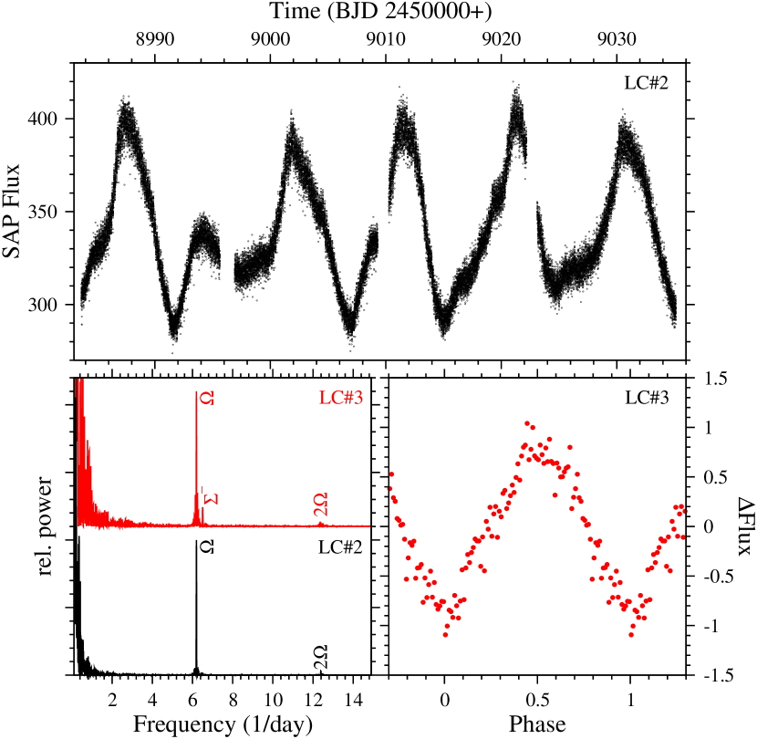
Figure 24: Light curve LC#2 (top), power spectra of LC#2 (black) and LC#3 (red) (lower left) and superhump waveform (lower right) of HS 0229.

The power spectra of all light curves contains a strong signal at the orbital frequency and a much weaker one at its first overtone. The lower left frame of Fig. 24 shows as examples the spectra of LC#2 and LC#3. The average value of the peak frequencies permits to improve the precision of the orbital period to 0.161439(9) d. The orbital waveform depends on the phase of the brightenings and will be explored in the upcoming paper mentioned above.

Apart from the orbital signal the power spectrum of LC#3 contains a small but significant peak at a slightly higher frequency. At a much fainter level (too faint to be conspicuous if it were not for its stronger appearance in LC#3) it is also detected in the other light curves. I take it as an indication of a negative superhump. It has the same period of 0.15369(3) d in LC#1 – LC#3, and a marginally lower one of 0.1534(1) in LC#4. Its waveform (lower left frame of Fig. 24) is almost sinusoidal.

3.18 HS 0506+7725

HS 0506+7725 (HS 0506 hereafter) is a cataclysmic variable also identified in the Hamburg Quasar Survey and studied by Aungwerojwit et al. (2005). They detected deep low states (see also the AAVSO long term light curve) which allow the system be be ranked among the VY Scl stars. The spectroscopic orbital period is 0.14770(14) d. This period was not detected in their light curves which otherwise are characterized by the strong random flickering common to VY Scl objects (Bruch, 2021).

TESS observed HS 0605 in eight sectors. The data can be combined into four 2-sector light curves, with an interval of 4 months between LC#1 and LC#2, and LC#3 and LC#4, respectively. LC#2 and LC#3 are separated by about two years. All light curves contain well expressed variations on times scales shorter than a day, superposed on modulations on longer time scales which, while not periodic, appear to have some regularity. This is best seen in LC#3 which is displayed together with LC#2 in the upper frames of Fig. 25.

Consequently, the power spectra contain many unstable signals at low frequencies. As an example, the power spectrum of LC#2 is reproduced in the lower left frame of Fig. 25. In none of the spectra a signal appears at the spectroscopic orbital frequency. Instead, the power spectrum of LC#2 (but not of the other light curves) contains a conspicuous signal at a slightly higher frequency corresponding to a period of 0.1417(1) d. The time resolved power spectrum (displayed in the third row of the figure together with the conventional power spectrum in a narrow frequency range around the signal) reveals that it is not permanent but appears only in a 16 d interval starting at JD 2449004 and possible returns right at the end of LC#2. I interpret it tentatively as being due to a temporarily active negative superhump. Within the elevated noise level the superhump waveform (lower right frame of Fig. 25) does not deviate much from a simple sine curve.

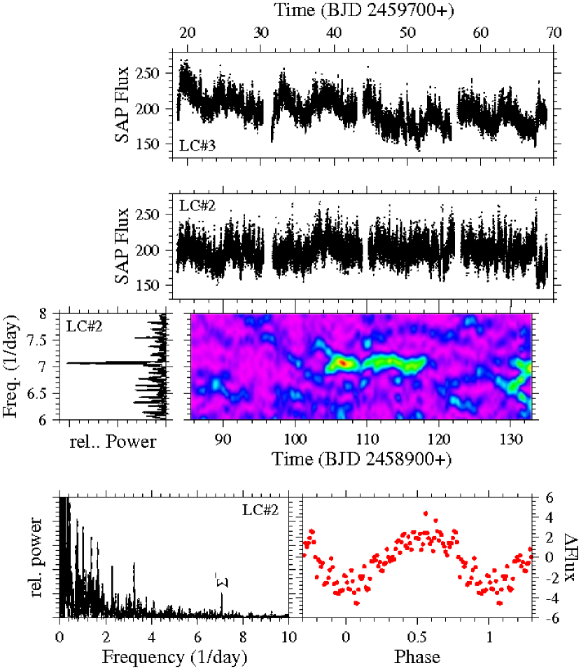
Figure 25: Top row: Light curve LC#3 of HS 0506. 2^nd and 3^rd row: Light curve of LC#2 and its power spectrum in a narrow range around the frequency of a temporarily active negative superhump in conventional and time resolved forms. Bottom row: Power spectrum of LC#2 in a wider frequency range (left) and the superhump waveform (right).

3.19 HS 0642+5049

HS 0652+5049 (HS 0642 hereafter) is still another object listed in the Hamburg Quasar Survey (HS) and identified as a cataclysmic variable by Aungwerojwit et al. (2005). They did not find radial velocity variations in their spectra, but the power spectrum of the combined light curves of the nights of October 25, December 8 and December 9, 2004 indicates a period of 0.156875(16) d.

Two single sector TESS light curves of HS 0642 are available, separated by 3 yrs (upper frames of Fig. 26). LC#1 exhibits clear variations on the time scales of 4 and 1 d, superposed upon more gradual variations. The yellow curve is a fit to the data of a fifth order polynomial (to follow the long term variations) and two sine terms with periods of $P_{1}=4.02$ d and $P_{2}=1.09$ d, respectively. Of course, these long periods also appear as strong peaks in the power spectrum (lower left frame of the figure). At higher frequencies the strongest peak corresponds to a period of 0.15791(2) d. Even considering the error limits this is incompatible with the orbital period of Aungwerojwit et al. (2005). But the respective frequency difference corresponds to a period of 24 d, close to the half the time difference of 45 d of the two observing mission on which their period is based. Thus, the period difference may well be due to the choice of a wrong alias peak by Aungwerojwit et al. (2005) (see their figure 13). Therefore, I consider 0.15791 d as the orbital period of HS 0642. The star then has a saw-tooth shaped orbital waveform (black dots in the second lower left frame of Fig. 26) with a slightly longer rise and a steeper decline.

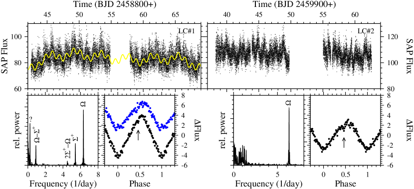
Figure 26: Top: Light curves of HS 0642. The yellow curve in the left frame is the sum of a fifth order polynomial and two sine waves with periods of 4.02 and 1.09 h fitted to the data. Bottom: Power spectra (left) and waveforms (right) for both light curves. Black and blue colours refer to orbital and SH variations, respectively. The arrows point to a faint but possibly persistent structure in the orbital waveform which repeats itself at exactly the same phase in both light curves.

Close to the orbital signal in the power spectrum another peak at a lower frequency can be interpreted as being to due to a positive superhump at a period of 0.18471(6) d (lower left frame of Fig. 26). A weaker close-by third peak is then identified as $2\Sigma^{+}-\Omega$, and the 1.09 d period is the beat period between the orbital and superhump variations. However, at $\epsilon=0.170$ the period excess lies much above the Stolz-Schoembs relation. This will be discussed in Sect. 4. The superhump waveform (blue dots in the figure), being saw-tooth shaped, is quite similar to the orbital waveform.

Light curve LC#2 (upper right frame of Fig. 26) also contains variations on time scale of one to a couple of days. However, in contrast to LC#1, they are not periodic. Instead, they generate a region of enhanced power in the range of 0.5 – 1.5 d^-1 (see the power spectrum in the lower frames of the figure). Otherwise, the power spectrum only contains a strong signal at the orbital frequency. The superhump has vanished. The orbital waveform has a lower amplitude than in LC#1 and a more sinusoidal shape. The small dip at phase 0.465 (marked by the arrow in the figure) may not be spurious, because the waveform constructed from LC#1 has a similiar, albeit fainter dip at exactly the same phase.

At a low power level a concentration of peaks appears in the power spectrum of LC#1 (but not of LC#2) between frequencies of about 10 and 14 d^-1 (left frame of Fig. 27). Two of these may be identified as the first overtones of the superhump and the orbital signal. The others, however, defy a simple explanation and seem to be unstable as is illustrated by the time resolved power spectrum in the right hand frame of the figure. Thus, HS 0642 is another member of the group of systems which exhibit QPOs on the time scale close to an hour.

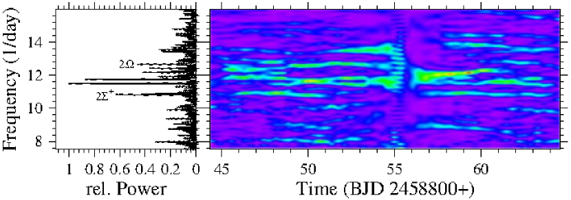
Figure 27: Power spectrum of LC#1 of HS 0642 in a narrow frequency range with a concentration of unstable signals in conventional (left) and time resolved form (right).

This leave just one significant power spectrum signal without explanation, i.e, the long 4.02 d period in LC#1. It cannot easily be related to any of the other periods in HS 0642 and its nature remains unknown.

3.20 IGR J08390-4833

Based on its optical spectrum Kniazev et al. (2008) identified IGR J08390-4833 (IGR J0839 hereafter) as a cataclysmic variable. In Chandra observations Sazonov (2008) detected X-ray pulsations with a period of $1450\pm 40$ sec and classified the system as an intermediate polar. Based on XMM-Newton observations Bernardini et al. (2012) refined this period to $1480.8\pm 0.5$ sec. A consistent period was also seen in the UV, but the $B$ band data yielded a period of $1650\pm 7$ sec which the authors interpreted as the orbital sideband of the WD spin period, implying a long orbital period of IGR J0839 of $8\pm 1$ h.

Two 2-sector TESS light curves separated by 2 years are available. They show that IGR J0839 is not only an intermediate polar but also exhibits negative superhumps, albeit not permanently. LC#2 (upper frame of Fig. 28) contains sinusoidal variations superposed upon more gradual variations. The yellow curve is the sum of a third order polynomial (for the gradual modulation) and a sine fit to the data. It already suggests being the beat between two other periods. This is confirmed by the power spectrum (lower left frame of the figure) which contains two peaks at neighbouring frequencies and a signal at their difference. The lower frequency peak, corresponding to a period of 0.25408(2) d, is orbital. This is obvious from the power spectrum of LC#1 which contains the same signal but not the one at the higher frequency, as well as from the analysis of the IP type variations (see below). The waveform of the orbital variations (black dots in the lower right frame of the figure) is close to a simple sine curve. The second peak in the power spectrum corresponds to a period of 0.24013(4) h. It can be interpreted as being due to a negative superhump. The beat period between orbit and superhump of 4.38(2) is reflected in the sine wave in the light curve. The superhump waveform (red dots in Fig. 28) consists of a single hump with a structured maximum. The superhump is not permanent because no trace of it can be detected in LC#1.

Although not the topic of this study, a brief discussion of the IP type variations in J0839 is in order. They are better expressed in LC#1 than in LC#2. The power spectrum (insert in the lower left frame of Fig. 28) contains only a faint signal at the frequency of the X-ray pulsations seen by Sazonov (2008) and Bernardini et al. (2012). Their period can be determined with much higher precision than based on the previous observations. I measured 1482.34(5) sec. Note that this is significantly longer than expected considering the error margin quoted by Bernardini et al. (2012). At optical wavelengths ($B$ band) these authors detected a longer period of 1560(7) sec which they take to be the orbital sideband of the WD spin period. No peak is seen at the corresponding frequency in the TESS power spectra. However, a signal much stronger than the WD spin signal corresponds to a period of 1589.603(9) sec. Adopting the orbital period derived above it is undoubtedly the orbital sideband $\omega-\Omega$ of the spin. Another signal can be identified as $\omega-2\Omega$. The same is true for the first overtone at $2\omega-2\Omega$ (beyond the limits of the figue) but not for the spin signal at $2\omega$. I cannot offer an explanation for the remarkable difference of almost 30 sec, much beyond the error margin, between the sideband period of 1560(7) sec quoted by Bernardini et al. (2012) and the 1589.603(9) sec period measured in the TESS data.

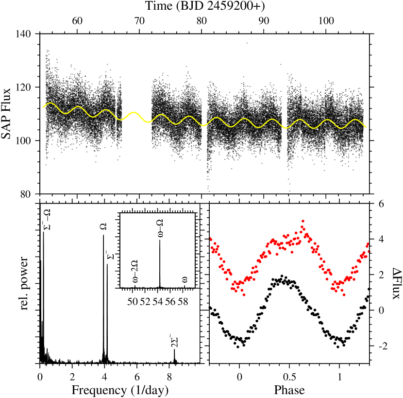
Figure 28: Light curve (top), power spectrum (lower left) and waveforms (lower right) of the orbital (black) and superhump variations (red) of LC#2 of IGR J0839. The insert in the lower left frame contains the power spectrum of LC#1 at higher frequencies showing the (weak) WD spin signal and its orbital sidebands. The continuous yellow curve in the upper frame is the sum of a low order polynomial (to follow the gradual variations) and a least squares sine fit to the data.

3.21 H$\alpha$ 103959.96-470126.1

H$\alpha$ 103959.96-470126.1 (H$\alpha$ 1039 hereafter) was identified as a cataclysmic variable by Pretorius & Knigge (2008) in a sample of H$\alpha$ emission line star from the AAO/UKST SuperCOSMOS H$\alpha$ Survey. They measured a spectroscopic orbital period of 0.1577(2) d.

TESS observed H$\alpha$ 1039 in two subsequent sectors. Just as in the case of KQ Mon (Sect. 3.10) Stefanov & Stevanov (2023) published their analysis of the same data when this study was in preparation. Therefore, the reader is referred to that paper for further details. I only add that the superhump waveform consists of a somewhat skewed single hump.

3.22 H$\alpha$ 112921.67-535543.6

H$\alpha$ 112921.67-535543.6 (H$\alpha$ 1129 hereafter) is another H$\alpha$ emission line star identified as a cataclysmic variable by Pretorius & Knigge (2008). The spectroscopic orbital period is 0.153546(2) d.

The single sector TESS light curve (upper frame of Fig. 29) indicates that this system exhibits negative and possibly simultaneously positive superhumps. It contains only slight variations on time scales of days above the noise level. The power spectrum (lower left frame of the figure) is dominated by a signal at the orbital frequency and its weaker first overtone. The waveform (lower right frame; back dots) consists of a single flat-topped hump. An amplified view of the orbital signal reveals some satellite lines (inset in the lower left frame of Fig. 29). Apart from the usual side-lobes close to the main peak, unavoidable in the power spectra of finite data sets, another maximum at a higher frequency, corresponding to a period of 0.14796(8) d, can be identified as being due to a negative superhump. A weaker peak close to 7.01 d^-1 is then the $2\Sigma^{-}-\Omega$ signal. The beat between orbital and superhump period is 4.1 d. Considering the uncertainties caused by the noise in the light curve a low frequency signal at 3.9 d may be a manifestation of the disk precession period. The superhump waveform (lower right frame of the figure; red dots) is noisy and undistinguishable from a simple sine curve.

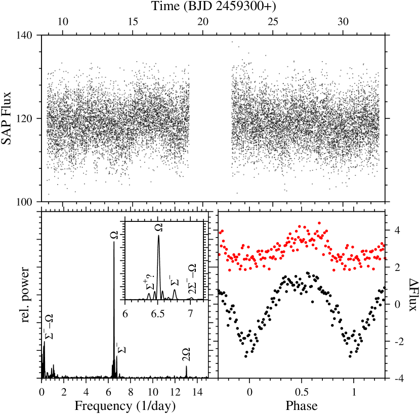
Figure 29: Light curve (top), power spectrum (lower left) and waveforms (lower right) of the orbital (back) and superhump variations (red) of H$\alpha$ 1129. The insert in the lower left frame contains a blow-up of the range around the orbital and superhump frequencies.

A power spectrum peak below the frequency of the orbital signal (inset in Fig. 29) corresponds to a period of 0.1571(1) d. Could this be caused by a positive superhump? The implied period excess of 0.023 is small but not drastically so considering the scatter in the superhump period – period excess relation (see Fig. 31). But then, H$\alpha$ 1129 would be the only system with positive and negative superhumps (simultaneously or not) where the period excess is smaller for the pSH than for the nSH. Therefore, I leave open the question whether the 0.1571 d period is caused by a superhump or some other mechanism.

3.23 ASASSN-14ix

The transient ASASSN-14ix remains an almost unstudied object. The only available information consists of informal communications (Hambsch, 2014a, b) reporting deep eclipses and an orbital period of 0.1444610954(1) d. The single sector TESS light curve (upper frame of Fig. 30) contains a $\approx$1 mag outburst and what appears the be the decline from a second outburst. Thus, ASASSN-14ix may be be a NL with brightenings such as, e.g., FY Per (see Sect. 3.12) or HS 0229 (Sect. 3.17) or even an outright dwarf nova.

The strongest signal in the power spectrum (lower left frame of Fig. 30) corresponds to a period of 0.1382(2) d, shorter than the orbital period. I take this as the manifestation of a negative superhump. The dynamical power spectrum shown in the second row of the figure together with the conventional spectrum in a small range around the orbital and superhump frequencies shows that the superhump signal subsides during the outburst. It persists during quiescence, vanishes abruptly right at the onset of the outburst, but does not wait until the end of the outburst to reappear. Instead, it restarts already just after outburst maximum.

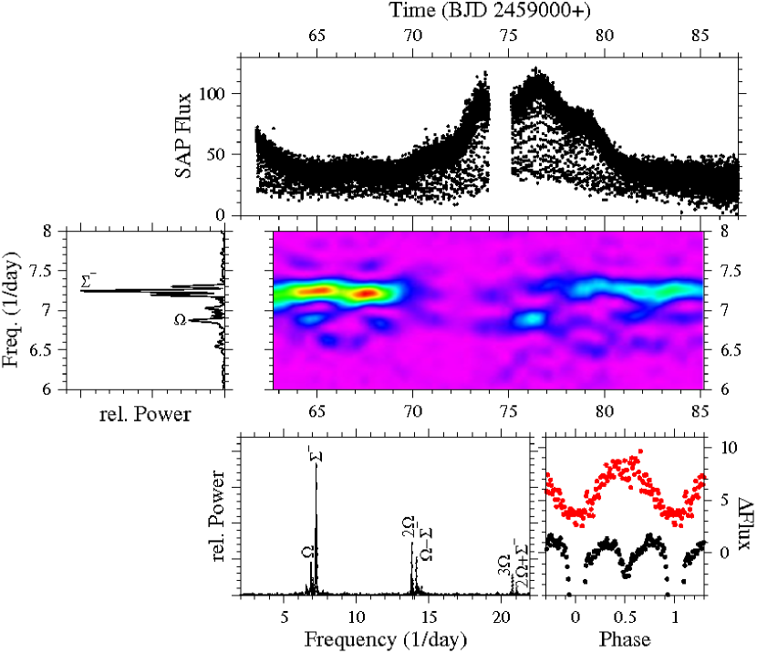
Figure 30: Top: Light curve of ASASSN-14ix. Middle: Power spectrum of the light curve (eclipses masked) in a narrow range around the orbital and superhump frequencies in the conventional (left) and time resolved forms (right). Bottom: Power spectrum in a wider frequency range (left) and the orbital (black) and superhump (red) waveforms (right).

The superhump waveform (lower right frame of Fig. 30; in red) cannot be distinguished from a simple sinusoid. The orbital waveform (in black) contains a well expressed secondary eclipse. Except for the depth of the primary eclipse it does not change significantly between quiescence and outburst.

4 Discussion

In Paper II, I presented a census of superhumps in NLs. The current study already supersedes it, enlarging the number of known SH systems among NLs by almost 50%. Moreover, SHs in other NLs have recently been reported in the literature. These are listed in Table 5. Some basic statistics of the entire sample of the superhump systems is given in Table 6, noting that in some of the newly added systems the presence of SHs still needs confirmation [LZ Mus (nSH); H$\alpha$ 1129 (pSH)], or their nature as either pSH or nSH requires clarification (DK Lac). While the previous census showed that the number of positive and negative superhump systems is approximately balanced, the new detections revealed 2.4 times more negative than positive SH systems. I cannot think of an observational bias to explain the preponderance of negative SH systems among the new detections. On the other hand, the lower than proportional growth rate of NLs showing both, pSHs and nSHs, or even both simultaneously, may be due to insufficient temporal coverage of the additional systems.

Table 5: Additional NLs identified as superhump systems.

Name	orb. period	nSH		pSH		Reference
	(d)	period (d)	$\epsilon$	period (d)	$\epsilon$
V598 Pup	0.162874	0.155	$-0.048$	–	–	1
YZ Ret	0.1324539			0.1384	0.045	1
BG Tri	0.15845(10)			0.1727(14)	0.090	2
Gaia DR3 4684361817175293440	0.15401(53)	0.14750(52)	$-0.042$	–	–	3
Gaia DR3 5931071148325476992	0.14827(46)	0.14248(43)	$-0.039$	–	–	3
HBHA 4204-09	0.14128(22)	0.13657(22)	$-0.033$	–	–	3
SDSS J090113.51+144707.6	0.14631(17)	0.13991(17)	$-0.044$	–	–	3
References: 1 = Schaefer (2022); 2 = Stefanov et al. (2022); 3 = Stefanov & Stevanov (2023)

Table 6: Basic statistics of superhump systems among NLs.

	Number
Total number of superhump systems	74
Positive superhump systems	37
Negative superhump systems	55
Systems with both, pSHs and nSHs	20
Systems with simultaneous pSHs and nSPs	11

The new data points warrant an update on the relationship between the superhump period excess $\epsilon=\left(P_{\rm SH}-P_{\rm orb}\right)/P_{\rm orb}$ and the superhump period $P_{\rm SH}$ (i.e., the Stolz-Schoembs relation, Stolz & Schoembs, 1984) for NLs. This is shown in the left frame of Fig. 31 for positive, and in the right frame for negative superhumps. The black dots represent data listed in table 4 of Paper II, while the red ones are the additional data points from Tables 3 and 5. The small orange dots in the left frame are taken from table 9 of Patterson et al. (2005) to serve as reference. Most of them represent SU UMa type dwarf novae in outburst which follow the Stolz-Schoembs relation much more closely than NLs. Moreover, the gradient of the relation is much steeper for dwarf novae than for NLs. The range of pSH periods measured in EI UMa (Sect. 3.14) and the two distinct nSH values of NS Cnc (Sect. 3.3), respectively, lead to points in the diagrams which are connected by a straight line.

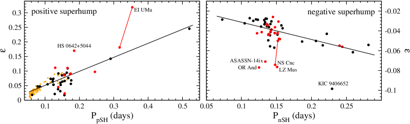
Figure 31: Period excess $\epsilon$ of superhumps as a function of the superhump period $P_{\rm SH}$ (Stolz-Schoembs relation). Left: Stolz-Schoembs relation for positive superhumps. Data listed in table 4 of Paper II are shown as black dots, while the red dots represent data from Tables 3 and 5 of this study. The extremes of the range of $\epsilon$ values measured in EI UMa are connected by a red line. The black line is a linear least squares fit to all data, excluding six low credential superhump systems identified in Paper II plus H$\alpha$ 1129, the strongly deviating HS 0642+5044, and the high $\epsilon$ point of EI UMa. For comparison, data taken from table 9 of Patterson et al. (2005) are plotted as smaller orange dots. Right: The same for negative superhumps. The red line connects the two SH period excess values measured in NS Cnc. The least squares fit to the data does not include the individually labelled stars and the low credential system RW Tri (Paper II).

Updated numerical expressions for the Stolz-Schombs relation were calculated as a least squares linear fit to the data, excluding the systems identified as low credential superhumpers in Paper II, as well as the pSH data point for H$\alpha$ 1129 which requires confirmation, the high $\epsilon$ point of EI UMa, the low $\epsilon$ point of NS Cnc, and the other individually identified stars in the figure. Expressing the relation in the original form as $\epsilon$ versus $P_{\rm SH}$, or alternatively as a function of $P_{\rm orb}$, we have for positive superhumps:

$$\epsilon = 0.003(3)+0.481(20)\times P_{\rm pSH}[{\rm h}]$$ (1)

$$\epsilon = 0.000(4)+0.540(26)\times P_{\rm orb}[{\rm h}]$$ (2)

and for negative superhumps

$$\epsilon = -0.014(9)-0.174(6)\times P_{\rm nSH}[{\rm h}]$$ (3)

$$\epsilon = -0.014(9)-0.165(6)\times P_{\rm orb}[{\rm h}]$$ (4)

It is striking that the negative superhumps in five stars (labelled in Fig. 31; right) have a period excess much below the sequence defined by the other systems. They almost appear to form a separate parallel lower sequence. The ratio between the observed and calculated (Eq. 3) period excess is 2.17 for OR And, 1.92 (ASASSN-14ix), 1.87 (NS Cnc), 1.91 (LZ Mus) and 1.78 (KIC 940652). Similarly, the high $\epsilon$ point of the positive superhump system EI UMa lies 1.870, times above the expected values (while the low point is not far from the overall relation). The corresponding value for HS 0642 is 1.88. Is it a coincidence that all these deviating period excesses are quite close to two times the values predicted by the Stolz-Schoembs relation? Doubling the period excess would occur if the disk precession period increases by a similar factor (the exact factor depends somewhat on the orbital period). This is dificult to envision. Alternatively, the observational manifestation of the superhumps may change such that their period changes by a factor of two. This may happen if the SH light source switches on and off, or becomes visible to the observer, either one or two times during each synodic orbit of the secondary around the eccentric or tilted accretion disk. However, I am not aware of any theoretical work or of simulations which support such a scenario. In this context it may be worthwhile to remind the reader of other unexpected relations between orbital, superhump and beat periods involving small integral numbers within their formal error margins, namely the supraorbital variations of V603 Aql (Bruch & Cook, 2018) and V1974 Cyg (Semeniuk et al., 1994, and Paper II) on twice, and possibly of RZ Gru (Paper I) on four times the calculated beat period between orbit and superhump. In the other extreme, supraorbital periods of half (OR And; Sect. 3.1) or a quarter (DK Lac; Sect. 3.9) of the calculated beat period are seen. Is this just numerology, or do these facts really tell us something about the physics of superhumps?

As is well known, theory predicts an upper limit to the mass ratio of CVs which can develop positive superhumps. The exact value is contested. Numbers between $q=M_{\rm sec}/M_{\rm prim}=0.22$ and 0.39 are quoted in the literature (Whitehurst & King, 1991; Pearson, 2006; Smak, 2020). Since on average the secondary star mass of CVs but not the WD mass increases with the orbital period, the average mass ratio also increases with period. Consequently, long period CVs should not exhibit positive superhumps. Yet, Fig. 31 contains four stars with an orbital period above 0.2 d. Two of these, KIC 9406653 and GZ Gru, have already been discussed in Paper II. The others are CN Vel and EI UMa. KIC 9406653 is a double lined spectroscopic binary with a securely measured mass ratio of $q=0.83$ (Gies et al., 2013). In the other cases no direct measurements of $q$ are available. But the semi-periodic mass-period relation of Knigge et al. (2011) permits to estimate the secondary star mass or to provide a lower limit. For CN Vel, $M_{\rm sec}$ is estimated to be 0.58 $M_{\odot}$. The orbital period of the remaining two systems lies above the upper limit of the list provided by Knigge et al. (2011) which ends at a period of 0.2468 d, corresponding to $M_{\sec}=0.7\,M_{\odot}$. I take this as a lower limit to the secondary star mass of EI UMa and RZ Gru. Assuming the primary star mass to be equal to the Chandrasekhar mass, lower limits of $q>0.39$ for CN Vel and $q>0.48$ for EI UMa and RZ Gru are derived. Thus, while superhumps in CN Vel are just barely compatible with theory, this is not true for the other three long period systems exhibiting positive superhumps, aggravating the problem outlined in Paper II.

In addition to superhumps, the power spectra of several of the stars of this study as well as in Papers I and II contain enhanced power within a more or less broad frequency range indicative of QPOs with periods on time scales of the order of an hour. Table 7 lists those systems together with the approximate range of periods. In addition to hourly time scale QPOs, HS 0642 also shows QPOs with quasi-periods of the order of a day, as does MV Lyr. QPOs in this period range would be difficult to detect in terrestrial observations but they show up in the long TESS (or Kepler) data trains. I am not aware that this phenomenon has been discussed in the literature. Since it is also not the topic of this study, I will refrain here from looking deeper into this issue. But it may well deserve some specific consideration in a dedicated publication.

Table 7: NLs exhibiting long period QPOs.

Name	Period range (h)	Reference
UU Aqr	2.15 …32.40	Paper II
TT Ari	0.25 …30.30	Paper I
BZ Cam	1.70 …33.00	Paper II
LS Cam	0.80 …30.85	This work
V592 Cas	0.15 …30.35	Paper II
V751 Cyg	0.35 …30.40	Paper II
BB Dor	0.25 …30.80	Paper II
RZ Gru	0.35 …31.20	Paper I
V533 Her	0.30 …30.70	Paper I
BH Lyn	3.40 …33.80	Paper II
MV Lyr	15.00 …23	Paper I
CP Pup	1.45 …31.65	Paper I
LN UMa	2.20 …32.70	This work
CN Vel	1.85 …32.50	This work
HS 0642	1.70 …32.40	This work
HS 0642	12.00 …36	This work

5 Summary

The analysis of the TESS light curves of all stars classified as novalike variables or old nova in the Ritter & Kolb catalogue (excluding AM Her type stars), and the TESS data of which have not been the subject of previous studies, revealed 19 systems to exhibit previously undetected superhumps. The scope of this study is exploratory, limited to the detection and the characterization of the basic properties of the superhumps of the new SH systems (i.e., their periods, their persistance or coming and going, their waveforms), including also the SH properties of four previously known or recently detected superhump systems. In many cases, a deeper investigation of the superhumps, their behaviour and their consequences for the structure of the individual binaries is warranted, but must await more specific studies than the present compilation can provide.

As a by-product the TESS data permitted to correct or to improve the orbital periods of more than half of the investigated systems. Additionally, further interesting features observed in the light curves are briefly mentioned. Together with similar properties seen in other stars of the entire Ritter & Kolb sample they will be the topic of future studies.

The new detections listed here, together with other recent discoveries of superhumps in NLs reported in the literature, all of them also based on TESS data, elevate the known number of SH systems among non dwarf novae CVs by more than 50%, emphasizing the enormous potential of long, (almost) uninterrupted data trains to reveal even low amplitude periodic variations on time scales comparable to typical nightly terrestrial light curves in the presence of often much stronger irregular variability auch as flickering, or in noisy light curves of faint stars. They also show that superhumps in NLs are more common than previously known.

Data availability

All data used in the present study are publically available at the Barbara A. Mikulski Archive for Space Telescopes (MAST:
https://mast.stsci.edu/portal/Mashub/clients/MAST/
Portal.html), the AAVSO web site (https://www.aavso.org) and the ASAS-SN web site (https://asas-sn.osu.edu).

References

- Aungwerojwit et al. (2005) Aungwerojwit A., Gänsicke B.T., Rodríguez-Gil P., et al., 2005, A&A, 443, 995
- Barlow et al. (2022) Barlow B.N., Corcoran K.A., Parker I.M., et al., 2022, ApJ, 928, 20
- Bernardini et al. (2012) Bernardini F., de Martino D., Falanga M., et al., 2012, A&A, 542, A22
- Bond (1979) Bond H.E., 1979, White Dwarfs and Variable Degenerate Stars, ed. H.M. van Horn, V. Weidemann, & M.P. Savedoff, IAU Coll. 53, p. 495
- Borucki et al. (2010) Borucki W.H., Koch D., Basrik G., et al., 2010, Science, 327, 977
- Bruch (2021) Bruch A., 2021, MNRAS, 503, 953
- Bruch (2022) Bruch A., 2022, MNRAS, 514, 4718
- Bruch (2023) Bruch A., 2023, MNRAS, 519, 352
- Bruch & Cook (2018) Bruch A., & Cook L.M., 2018, New Astr., 63, 1
- Deeming (1975) Deeming T.J., 1975, Ap&SS, 39, 137
- Dobrzycka et al. (1998) Dobrzycka D, Dobrzycki A., Engels D., & Hagen H,-J., 1998, AJ, 115, 1634
- Gänsicke et al. (2002) Gänsicke B.T., Hagen H.-J., Kube J., et al., 2002, The Physics of Cataclysmic Variables and Related Objects, eds. B.T. Gänsicke, K. Beuermann, & K. Reinsch, ASP Comf. Ser., 161, p. 623
- Gaia Collaboration (2020) Gaia Collaboration, 2022, A&A, 649, A1
- Gies et al. (2013) Gies D.R., Guo Z., Howell, S.B., 2013, ApJ, 775, 64
- Gülseçen & Esenoglu (2014) Gülseçen H., & Esenoglu H., 2014, New Astr., 144, 81
- Hambsch (2014a) Hambsch F.-J., 2014a, http://ooruri.kusastro.kyoto-u.ac.jp/mailarchive/vsnet-alert/18036
- Hambsch (2014b) Hambsch F.-J., 2014b, http://ooruri.kusastro.kyoto-u.ac.jp/mailarchive/vsnet-alert/18077
- Hameury (2020) Hameury J.-M., 2020, AdSpR, 66, 1004
- Hameury et al. (2022) Hameury J.-M., Lasota, J.-P., & Shaw A.W., 2022, A&A, 665, A7
- Hillwig et al. (1998) Hillwig T.C., Robertson J.W., & Honeycutt R.K., 1998, AJ, 115, 2044
- Honeycutt (2001) Honeycutt R.K., 2001, PASP, 113, 473
- Honeycutt & Kafka (2004) Honeycutt R.K., & Kafka S., 2004, AJ, 128, 1279
- Kato et al. (2001) Kato T., Uemura M., Ishioka R., & Kinnunen T., 2001, PASJ, 53, 1185
- Katysheva & Shugarov (2008) Katysheva N.A., & Shugarov S.Yu. 2008, ASP Conf. Ser., 372, 15th European Workshop on White Dwarfs, eds. R. Napivotzki & M.R. Burleigh, 523
- Kniazev et al. (2008) Kniazev A., Revnivtsev M., Sazonov S., Burenin A., & Tekola A., 2008, ATel, 1488
- Knigge et al. (2011) Knigge C., Baraffe I., & Patterson J., 2011, ApJS, 194, 28
- Kozhevnikov (2010) Kozhevnikov V.P., 2010, Astr. Lett., 36, 554
- Li et al. (2017) Li K, Hu S.-M., Zhou J.-L., et al., 2017, PASJ, 69, 28
- Liller (1980) Liller M.H., 1980, IBVS, 1743
- Littlefield et al. (2022) Littlefield C., Lasota J.-P., Hameury J.-M., et al., 2022, ApJL, 924, 8
- Lomb (1977) Lomb N.T., 1976, Ap&SS, 39, 447
- Mickaelian et al. (2002) Mickaelian A.M., Balayan S.K., Ilovaisky S.A., et al., 2002, A&A, 381, 894
- Papadaki et al. (2009) Papadaki C., Boffin H.M.J., Stanishev V., et al., 2009, J. Astr. Data, 15,1
- Patterson et al. (2002) Patterson J., Fenton W.H., Thorstensen J.R., et al., 2002, PASP, 114, 1364
- Patterson et al. (2005) Patterson J., Kemp J., Harvey D.A., et al., 2005, PASP, 117, 1204
- Pearson (2006) Pearson K.J., 2006, MNRAS, 371, 235
- Peters & Thorstensen (2006) Peters C.S., & Thorstensen J.R., 2006, PASP, 118, 687
- Piirola et al. (2008) Piirola V., Vornanen T., Berdyugin A., & Coyne G.V., 2008, ApJ, 684, 553
- Pretorius & Knigge (2008) Pretorius M.L., & Knigge C., 2008, MNRAS, 385, 1471
- Rawat et al. (2022) Rawat N., Pandey J.C., Joshi A., & Yadawa U., 2022, MNRAS, 512, 6054
- Retter et al. (1996) Retter A., Leibowitz E.M., & Naylor T., 1999, MNRAS, 308, 140
- Retter et al. (1998) Retter A., Liller W., & Garradd G., 1998, IAU Circ., 7124
- Ricker et al. (2014) Ricker G.R., Winn J.N., Vanderspek R., et al., 2014, J. Astr. Tel. Instr. & Systems, 1, 014003
- Ringwald (1993) Ringwald F.A., 1993, The Cataclysmic Variables from the Palomar-Green Survey, PhD thesis, Dartmouth College
- Ritter & Kolb (2003) Ritter H., & Kolb U., 2003, A&A, 404, 301
- Rodríguez-Gil et al. (2007a) Rodríguez-Gil P., Gänsicke B.T., Hagen H.-J., et al., 2007a, MNRAS, 377, 1747
- Rodríguez-Gil et al. (2009) Rodríguez-Gil P., Martínez-Pais I.G., & de la Cruz Rodríguez I.G., 2009, MNRAS, 395, 973
- Rodríguez-Gil et al. (2007b) Rodríguez-Gil P., Schmidtobreick L., & Gänsicke B.T., 2007b, MNRAS, 374, 1359
- Rodríguez-Gil & Torres (2005) Rodríguez-Gil P., & Torres M.A.P., 2005, A&A, 431, 289
- Savitzky & Golay (1964) Savitzky A., & Golay M.J.E., 1964, Analytical Chemistry, 36, 1627
- Sazonov (2008) Sazonov S., Revnivtsev M., Burenin R., et al., 2008, A&A, 487, 509
- Scargle (1982) Scargle J.D., 1982, ApJ, 263, 853
- Scaringi et al. (2022a) Scaringi S., Groot P.J., Knigge C., et al., 2022a, Nature, 604, 447
- Scaringi et al. (2022b) Scaringi S., Groot P.J., Knigge C., et al., 2022b, MNRAS, 514, L11
- Schaefer (2022) Schaefer B.E., 2022, MNRAS, 517, 3640
- Schmidtobreick et al. (2005) Schmidtobreick L., Tappert C., Galli L., & Whiting A., 2005, IBVS, 5627
- Schwarzenberg-Czerny (1991) Schwarzenberg-Czerny A., 1991, MNRAS, 253, 198
- Semeniuk et al. (1994) Semeniuk I., Pych W., Olech A., & Ruszkowski M., 1994 Acta Astr., 44, 277
- Shafter & Ulrich (1982) Shafter A.W., & Ulrich R.K., 1982, Bull. AAS, 14, 880
- Shears et al. (2016) Shears J., Gänsicke B.T., Rodríguez-Gil P., et al., 2016, J. Brit. Astron. Assoc., 126, 42
- Sing et al. (2004) Sing D.K., Howell S.B., Szkody P., & Cordova F.A., 2004, PASP, 116, 1056
- Sion & Guinan (1982) Sion E.M., & Guinan E.G., 1982, Advances in Ultraviolet Astronomy. Four Years of IUE Research, ed. Y. Kondo, J.M. Mead, & R.D. Chapman, NASA CP-2238, p. 460
- Smak (2020) Smak, J. 2020, Acta Astron., 70, 313
- Stefanov & Stevanov (2023) Stefanov S.Y., Latev G., Boeva S., & Moyseev M., 2022, MNRAS, 516, 2775
- Stefanov et al. (2022) Stefanov S.Y., Stefanov A.K., 2023, MNRAS, 520, 3187
- Stolz & Schoembs (1984) Stolz V., Schoembs R., 1984, A&A, 132, 187
- Szkody et al. (2004) Szkody P., Henden A., Agüeros M., et al., 2006, AJ, 131, 973
- Tappert et al. (2013) Tappert C., Schmidtobreick L., Vogt N., & Ederoclite A., 2013, MNRAS, 436, 2412
- Thorstensen (1986) Thorstensen J.R., 1986, AJ, 91, 940
- Thorstensen et al. (2017) Thorstensen J.R., Ringwald A.F., Taylor C.J., et al., 2017, RNAAS, 1, 29
- Thorstensen et al. (2015) Thorstensen J.R., Taylor C.J., & Peters C.S., 2015, AJ, 149, 128
- Warner (1995) Warner B., 1995, Cataclysmic Variable Stars, Cambridge University Press, Cambridge
- Warner (2002) Warner B., & Woudt P.A., 2002, PASP, 114, 1222
- Wenzel (1987) Wenzel W., 1987, IBVS, 3086
- Whitehurst & King (1991) Whitehurst R., King A., 1991, MNRAS, 249, 25
- Wolfe et al. (2013) Wolfe A., Sion E.M., & Bond H.E., 2013, AJ, 145, 168
- Worpel et al. (2020) Worpel H., Schwope A.D., Traulsen I., Mukai K., & Ok S., 2020, A&A, 639, A17