Quasioptimal alternating projections and their use in low-rank approximation of matrices and tensors

Abstract

We study the convergence of specific inexact alternating projections for two non-convex sets in a Euclidean space. The $\sigma$-quasioptimal metric projection ($\sigma\geq 1$) of a point $x$ onto a set $A$ consists of points in $A$ the distance to which is at most $\sigma$ times larger than the minimal distance $\mathrm{dist}(x,A)$. We prove that quasioptimal alternating projections, when one or both projections are quasioptimal, converge locally and linearly for super-regular sets with transversal intersection. The theory is motivated by the successful application of alternating projections to low-rank matrix and tensor approximation. We focus on two problems—nonnegative low-rank approximation and low-rank approximation in the maximum norm—and develop fast alternating-projection algorithms for matrices and tensor trains based on cross approximation and acceleration techniques. The numerical experiments confirm that the proposed methods are efficient and suggest that they can be used to regularise various low-rank computational routines.

Keywords: alternating projections, quasioptimality, super-regular sets, matrices and tensors, low-rank approximation, nonnegativity, maximum norm

MSC2020: 15A23, 15A69, 49M20, 65F55, 65K10, 90C30

1 Introduction

1.1 Alternating projections

A recurring problem in mathematics is to find a point in a subset $A$ of a Euclidean space $H$. Consider a simple and illustrative example: solve a system of linear equations. When the matrix of the system is square and invertible, the solution set is a singleton. For an underdetermined system with a full-rank matrix, the solutions form an affine subspace, and we typically choose the (unique) solution of the smallest norm.

The latter is a particular case of a so-called metric projection of a point $x\in H$ onto a set:

$$\Pi_{A}(x)=\big{\{}a\in A\leavevmode\nobreak\ :\leavevmode\nobreak\ |x-a|=\inf\nolimits_{\hat{a}\in A}|x-\hat{a}|\big{\}}.$$ (1)

Indeed, the least-norm solution to a system of linear equations corresponds to the metric projection of the zero vector onto the affine subspace of all solutions. Moreover, this solution can be expressed in closed form via the QR decomposition of the matrix.

For more complex sets, it is no longer evident how to represent the metric projection. Suppose we want to find a point in the intersection of two ‘simple’ sets. Von Neumann proved [107, Theorem 13.7] that if $A$ and $B$ are linear subspaces then the sequence of alternating projections

$$b_{n+1}\in\Pi_{B}(a_{n}),\quad a_{n+1}\in\Pi_{A}(b_{n+1}),\quad n\geq 0,$$

started with $a_{0}\in\Pi_{A}(x)$ converges to $\Pi_{A\cap B}(x)$ for every $x\in H$. Later, it was shown that the global convergence of the sequence to $A\cap B$ holds for closed convex sets [13, 11] and that there is local convergence to $A\cap B$ for a class of closed non-convex sets [66].

This basic framework finds numerous practical applications in systems of linear inequalities [2, 75], overdetermined systems of linear equations [100], design of frames [103], compressed sensing [52], phase retrieval [6] and finance [54]; find more in [33].

1.2 Low-rank approximation with constraints

Our interest is in low-rank approximation of matrices and higher-order tensors with constraints [112, 15, 43, 45]. The best low-rank approximation of a matrix is given by its truncated singular value decomposition (SVD), and we can impose the additional constraints with the method of alternating projections [16]. For tensors, there are no general ways to represent even the best rank-one approximation [23, 111], and the direct minimisation of the Euclidean distance has a complicated optimisation landscape.

It is still possible to use the alternating projections to compute constrained low-rank approximations of tensors in subspace-based formats. The set of order-$d$ tensors with low Tucker ranks [61] is the intersection of $d$ sets of low-rank matrices corresponding to the $d$ unfoldings. Therefore, the projections can be alternated between the $d$ low-rank sets and the constraint set. This approach was taken in [59] to compute low-rank nonnegative approximations, but it has a major drawback: at no time during the iterations do we actually encounter a low-rank tensor, it is reached only in the limit. This is in contrast to the matrix case, where we work with a sequence of low-rank matrices that converges to the set of constraints and that we can halt once the constraints are almost satisfied.

While it is infeasible to compute the metric projection of an order-$d$ tensor onto the set of tensors with low Tucker ranks, there are SVD-based methods to construct good approximations that are at most $\sqrt{d}$ times worse than the best approximation [22]. In our previous work [101], we used this SVD-based procedure in place of the metric projection to compute low-rank nonnegative approximations of tensors in the alternating-projections fashion. Similar to the matrix case, this approach produces a sequence of low-rank tensors, and the numerical experiments showed convergence to the nonnegative orthant.

1.3 Inexact metric projections

The above example of low-rank tensor approximation highlights the need to generalise the notion of metric projections in order to admit points that might not attain the minimal distance but are within a constant factor from it.

This generalisation is also inevitable once we begin to consider the practical side of computations: every projection we compute numerically is inherently inexact. There are three main sources of inexactness: the floating-point arithmetic, the termination of iterative algorithms, and the algorithms that are not designed to be exact.

In low-rank tensor approximation, the three aspects act in unison. At the bottom level, all basic operations of linear algebra are subject to round-off errors in the floating-point arithmetic [53]. They are then used as building blocks in the numerical algorithms for the SVD, which are iterative and run until the tolerable error is reached [24]. Finally, algorithms akin to [22] use the SVD to compute quasioptimal low-rank approximations.

1.4 Contributions: Brief version

For $\sigma\geq 1$, we define the $\sigma$-quasioptimal metric projection of a point $x\in H$ onto $A$ as

$$\Pi_{A}(x;\sigma)=\{a\in A\leavevmode\nobreak\ :\leavevmode\nobreak\ |x-a|\leq\sigma\cdot\inf\nolimits_{\hat{a}\in A}|x-\hat{a}|\}.$$ (2)

The algorithm from [22] then computes an element of the $\sqrt{d}$-quasioptimal metric projection onto the set of low-rank order-$d$ tensors in the Tucker format (assuming that the SVD is exact), and the definition coincides with the optimal metric projection $\Pi_{A}(x)$ when $\sigma=1$.

We propose the method of quasioptimal alternating projections for two sets $A$ and $B$, quasioptimality constants $\sigma_{A}\geq 1$ and $\sigma_{B}\geq 1$, and the initial condition $a_{0}\in A$:

$$b_{n+1}\in\Pi_{B}(a_{n};\sigma_{B}),\quad a_{n+1}\in\Pi_{A}(b_{n+1};\sigma_{A}),\quad n\geq 0.$$ (3)

Following the ideas of Lewis, Luke and Malick [66], we prove local and linear convergence of the sequence to $A\cap B$ when $\sigma_{A}\geq 1$ with $\sigma_{B}=1$ (Theorem 6.3 and Corollary 6.4) and when $\sigma_{A}>1$ with $\sigma_{B}>1$ (Theorem 6.6). In both cases, we estimate the rate of convergence and the admissible values of $\sigma_{A}$ and $\sigma_{B}$. Our theorems also show that the sequence (3) converges to the quasioptimal metric projections of $a_{0}$ onto $B$ and $A\cap B$; see also Theorem 6.7. This is an improvement over [66, Theorem 5.2].

Consider the coordinate axes in the plane (Fig. 1). The Pythagorean theorem ensures that

$$\frac{|a_{1}|}{|a_{0}|}\leq\sqrt{\sigma_{A}^{2}-1}\cdot\sqrt{\sigma_{B}^{2}-1}$$

for every $b_{1}\in\Pi_{B}(a_{0};\sigma_{B})$ and $a_{1}\in\Pi_{A}(b_{1};\sigma_{A})$. Hence, the iterations converge if the right-hand side is below one. Theorem 6.6 captures this behaviour and extends it to non-convex sets with a non-orthogonal intersection. Note that the method might still converge even if the right-hand side is greater than one: everything depends on the particular instances of $b_{n+1}\in\Pi_{B}(a_{n};\sigma_{B})$ and $a_{n+1}\in\Pi_{A}(b_{n+1};\sigma_{A})$ that are computed during the iterations.

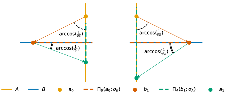
Figure 1: Quasioptimal alternating projections for two perpendicular lines in the plane converge when $\sqrt{\sigma_{A}^{2}-1}\cdot\sqrt{\sigma_{B}^{2}-1}<1$ and can diverge otherwise.

In numerical experiments, we compute constrained low-rank approximations with the quasioptimal alternating projections. First, we use them to impose nonnegativity on the approximations and show how a single iteration helps to regularise Riemannian matrix completion. Second, we develop a method to obtain low-rank approximations with small entrywise errors; we employ it to approximate orthogonal matrices and reconstruct tensors with quantised entries.

1.5 Outline

Our article could be of interest to two different communities; to reach out to both, we deliberately choose to make the presentation detailed and include the necessary background material on non-smooth optimisation and low-rank approximations.

The first, theoretical, part of the paper addresses the convergence of quasioptimal alternating projections (3), extending the analysis of [66] to quasioptimal metric projections (2). The second, numerical, part continues the investigation of [59, 101] on using alternating projections to compute nonnegative low-rank matrix and tensor approximations (which motivated our theory), and introduces a new application of alternating projections to low-rank approximation in entrywise norms.

In Section 2, we collect some preliminary results that are useful in the convergence analysis of alternating projections. We then revisit the main contributions of the paper in more details in Section 3 and compare them with the existing literature in Section 4. The properties of quasioptimal metric projections are studied in Section 5. The following Section 6 is devoted to the method of quasioptimal alternating projections and its local convergence for non-convex sets. Two applications of the method to low-rank matrix and tensor approximation are considered in Section 7. Some auxiliary results, proof details, and a summary of fast low-rank approximation methods can be found in the appendix.

2 Preliminaries and notation

Throughout the text, $H$ is a Euclidean space with inner product $\langle\cdot,\cdot\rangle$ and norm $|\cdot|$. The open unit ball at the origin and the open ball of radius $r>0$ centred at $x\in H$ are written as ${{\mathbb{B}}}=\{x\in H\leavevmode\nobreak\ :\leavevmode\nobreak\ |x|<1\}$ and ${{\mathbb{B}}}_{r}(x)=x+r{{\mathbb{B}}}$. We say that a set $\mathcal{V}\subseteq H$ is a neighbourhood of $x\in H$ if $\mathcal{V}$ is open and contains $x$. For a set $A\subseteq H$, let $\overline{A}$ denote its closure, $\mathrm{int}A$ its interior and $\mathrm{bdr}A$ its boundary. A non-empty set $A$ is called (i) locally closed at $\hat{a}\in A$ if there exists a neighbourhood $\mathcal{V}\subseteq H$ of $\hat{a}$ such that $A\cap\mathcal{V}$ is closed in $\mathcal{V}$; (ii) convex if for every $a_{1},a_{2}\in A$ and $\alpha\in(0,1)$ their combination $\alpha a_{1}+(1-\alpha)a_{2}$ is in $A$; (iii) a cone if for every $a\in A$ and $\alpha\geq 0$ their product $\alpha a$ is in $A$.

2.1 Metric projections

For a non-empty set $A\subseteq H$ and a point $x\in H$, we define the distance from $x$ to $A$:

$$\mathrm{dist}(x,A)=\inf\nolimits_{a\in A}|x-a|.$$

With this notation, we can rewrite the definition of the optimal metric projection (1):

$$\Pi_{A}(x)=\{a\in A\leavevmode\nobreak\ :\leavevmode\nobreak\ |x-a|=\mathrm{dist}(x,A)\}.$$

For $x\in A$, the optimal metric projection is obviously a singleton $\Pi_{A}(x)=\{x\}$. In general, however, there can be points $x\in H$ such that $\Pi_{A}(x)$ is empty. The following lemma ties the existence of optimal metric projections with the local topological properties of the set.

Lemma 2.1.

Let $A\subseteq H$ be non-empty and $\hat{a}\in A$.

1. Let $\mathcal{V}\subseteq H$ be a neighbourhood of $\hat{a}$ such that every $x\in\mathcal{V}$ has a non-empty optimal metric projection $\Pi_{A}(x)$. Then $A\cap\mathcal{V}$ is closed in $\mathcal{V}$.

2. Let $A\cap{{\mathbb{B}}}_{r}(\hat{a})$ be closed in ${{\mathbb{B}}}_{r}(\hat{a})$. Then for each $x\in{{\mathbb{B}}}_{r/2}(\hat{a})$ the optimal metric projection $\Pi_{A}(x)$ is non-empty and $|\pi-\hat{a}|\leq 2|x-\hat{a}|<r$ for every $\pi\in\Pi_{A}(x)$.

Proof.

This is a folklore result; we prove it in Appendix B for completeness. ∎

2.2 Normal cones

The concept of an ‘outward’ normal to a set is one of the central notions of variational analysis, which is used to formulate optimality criteria for constrained optimisation problems. From the perspective of alternating projections, we can learn a lot about the relative positions of two sets by comparing their specific ‘outward’ normal directions.

Let $A\subseteq H$ be non-empty and $\hat{a}\in A$. We say that $v\in H$ is a proximal normal to $A$ at $\hat{a}$ if there exists $\tau>0$ such that $\hat{a}\in\Pi_{A}(\hat{a}+\tau v)$. Let $N^{\mathrm{prox}}_{A}(\hat{a})$ denote the collection of all proximal normals to $A$ at $\hat{a}$:

$$N^{\mathrm{prox}}_{A}(\hat{a})=\{v\in H\leavevmode\nobreak\ :\leavevmode\nobreak\ \hat{a}\in\Pi_{A}(\hat{a}+\tau v)\text{ for some }\tau>0\}.$$

The set $N^{\mathrm{prox}}_{A}(\hat{a})$ is a convex cone, known as the proximal normal cone to $A$ at $\hat{a}$. If $x\in H$ has a non-empty optimal metric projection $\Pi_{A}(x)$, then $x-\pi\in N^{\mathrm{prox}}_{A}(\pi)$ for each $\pi\in\Pi_{A}(x)$.

Assume, in addition, that $A$ is locally closed at $\hat{a}$. Then $v\in H$ is a limiting normal to $A$ at $\hat{a}$ if there exists a sequence of points $(a_{n})\subset A$ and a corresponding sequence of proximal normals $(v_{n})\subset H$ with $v_{n}\in N^{\mathrm{prox}}_{A}(a_{n})$ such that $a_{n}\to\hat{a}$ and $v_{n}\to v$ as $n\to\infty$. The set $N^{\mathrm{lim}}_{A}(\hat{a})$ of all limiting normals to $A$ at $\hat{a}$ is a closed cone and is called the limiting normal cone to $A$ at $\hat{a}$.

Clearly, $N^{\mathrm{prox}}_{A}(\hat{a})\subseteq N^{\mathrm{lim}}_{A}(\hat{a})$, and the inclusion can be strict (see Fig. 2 and note that $N^{\mathrm{prox}}_{A}(\hat{a})=\{0\}$). It can also be shown that we can replace the proximal normals with limiting normals in the definition of the limiting normal cone:

$$N^{\mathrm{lim}}_{A}(\hat{a})=\{v\in H\leavevmode\nobreak\ :\leavevmode\nobreak\ \text{there are }A\ni a_{n}\to\hat{a}\text{ and }N^{\mathrm{lim}}_{A}(a_{n})\ni v_{n}\to v\text{ as }n\to\infty\}.$$ (4)

Another useful property of the limiting normal cone is how it distinguishes between interior and boundary points of the set: $N^{\mathrm{lim}}_{A}(\hat{a})=\{0\}$ if and only if $\hat{a}\in\mathrm{int}A$. Find a more in-depth discussion of proximal and limiting normal cones in [73, 89].

2.3 Super-regular sets

When we think of normal cones, it is customary to imagine them pointing in the ‘opposite’ direction from the set; indeed, this is what happens for smooth manifolds and convex sets. In general, this picture can be misleading as a simple example shows.

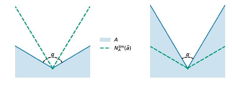
Figure 2: Limiting normal cones can point in the ‘opposite’ direction from the set.

Consider a closed concave set $A\subset\mathbb{R}^{2}$ with an angle of size $\alpha$ and let $\hat{a}$ be its vertex (see Fig. 2). When $\alpha>\frac{\pi}{2}$, the limiting normal cone $N^{\mathrm{lim}}_{A}(\hat{a})$ does point ‘away’ from $A$, but it still forms acute angles with some of the inward-looking directions. For smaller angles $\alpha\leq\frac{\pi}{2}$, the limiting normals themselves point ‘into’ $A$.

A class of sets that do not suffer from such shortcomings was introduced in [66]. Let $A\subseteq H$ be non-empty and locally closed at $\hat{a}\in A$. The set $A$ is called super-regular at $\hat{a}$ if for every $\varepsilon>0$ there exists $\delta>0$ such that $A\cap{{\mathbb{B}}}_{\delta}(\hat{a})$ is closed in ${{\mathbb{B}}}_{\delta}(\hat{a})$ and

$$\langle v,a^{\prime}-a\rangle\leq\varepsilon|v|\cdot|a^{\prime}-a|\quad\text{for all}\quad a,a^{\prime}\in A\cap{{\mathbb{B}}}_{\delta}(\hat{a})\quad\text{and}\quad v\in N^{\mathrm{lim}}_{A}(a).$$ (5)

Essentially, a set is super-regular at a point if, in its sufficiently small neighbourhood, each limiting normal forms an ‘almost’ obtuse angle with every direction that points into the set. The super-regularity property is shared, among others, by smooth manifolds and convex sets.

In the presence of super-regularity, the behaviour of the optimal metric projections improves locally. In general, the triangle inequality guarantees only that $|\pi-a|\leq 2|x-a|$ for $\pi\in\Pi_{A}(x)$. When the set is super-regular, the optimal metric projections are nearly non-expansive.

Lemma 2.2.

Let $A\subseteq H$ be non-empty and super-regular at $\hat{a}\in A$. Then for every $\varepsilon>0$ there exists $\delta>0$ such that for every $x\in{{\mathbb{B}}}_{\delta/2}(\hat{a})$ and each $\pi\in\Pi_{A}(x)$ it holds that

$$|\pi-a|\leq(1+\varepsilon)\cdot|x-a|\quad\text{for every}\quad a\in A\cap{{\mathbb{B}}}_{\delta}(\hat{a}).$$

Proof.

See [51, Theorem 2.14]. ∎

2.4 Transversal intersection of sets

Whether we can find a common point of two sets with the help of alternating projections, depends on how the sets are oriented relative to each other. Consider a two-dimensional example in Fig. 3. The two sets are the piecewise linear curve $A$ and the horizontal axis $B$, and they intersect at the origin. No matter the starting point and the order of the projections, the method of alternating projections either gets stuck in a loop or converges in one step. The latter takes place for the starting points on the vertical axis: all of them when we begin with $B$, and those in the lower halfspace when we begin with $A$. Therefore, the alternating projections fail to produce the common point of $A$ and $B$ for almost every starting point.

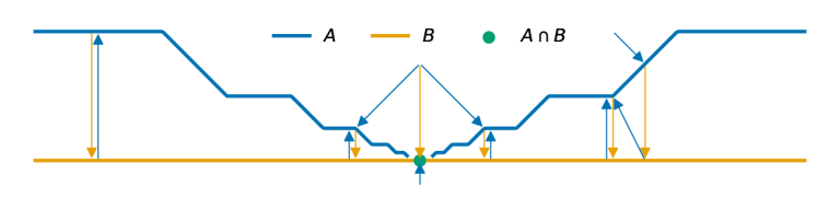
Figure 3: For certain pairs of sets $A$ and $B$, the alternating projections do not converge to $A\cap B$ for almost every starting point.

The following definition aims to rule out such pathological cases. Consider a pair of non-empty sets $A,B\subseteq H$ with a common point $\overline{x}\in A\cap B$, where both sets are locally closed. We say that $A$ and $B$ intersect transversally at $\overline{x}$ if

$$-N^{\mathrm{lim}}_{A}(\overline{x})\cap N^{\mathrm{lim}}_{B}(\overline{x})=\{0\}.$$

While we follow the terminology of [31], this property has other names in the literature, such as strong regularity [51] and linearly regular intersection [66]. See also [62].

The ‘quality’ of the intersection of two sets at a point can also be quantified:

$$\cos(A,B,\overline{x})=\max\big{\{}\langle u,v\rangle\leavevmode\nobreak\ :\leavevmode\nobreak\ u\in-N^{\mathrm{lim}}_{A}(\overline{x})\cap\overline{{{\mathbb{B}}}},\leavevmode\nobreak\ v\in N^{\mathrm{lim}}_{B}(\overline{x})\cap\overline{{{\mathbb{B}}}}\big{\}}.$$

This value lies in the interval $[0,1]$ and generalises the cosine of the angle between two linear subspaces. The following lemmas show the relationship between $\cos(A,B,\overline{x})$ and transversality; find their proofs in [66, 85].

Lemma 2.3.

Let two non-empty sets $A,B\subseteq H$ have a common point $\overline{x}\in A\cap B$, where both sets are locally closed. They intersect transversally at $\overline{x}$ if and only if $\cos(A,B,\overline{x})<1$.

Lemma 2.4.

Let two non-empty sets $A,B\subseteq H$ have a common point $\overline{x}\in A\cap B$, where both sets are locally closed. Assume that $\cos(A,B,\overline{x})<c$ for some $c\in(0,1]$. Then there is a neighbourhood $\mathcal{V}\subseteq H$ of $\overline{x}$ such that for every $a\in A\cap\mathcal{V}$ and $b\in B\cap\mathcal{V}$ the following holds:

$$\langle u,v\rangle<c\quad\text{for all}\quad u\in-N^{\mathrm{lim}}_{A}(a)\cap\overline{{{\mathbb{B}}}}\quad\text{and}\quad v\in N^{\mathrm{lim}}_{B}(b)\cap\overline{{{\mathbb{B}}}}.$$

3 Contributions: Detailed version

Recall the definition (2) of the $\sigma$-quasioptimal metric projection:

$$\Pi_{A}(x;\sigma)=\{a\in A\leavevmode\nobreak\ :\leavevmode\nobreak\ |x-a|\leq\sigma\cdot\mathrm{dist}(x,A)\}.$$

It serves to describe a wide range of inexact projections that appear in applications; primarily, we are motivated by low-rank approximations of higher-order tensors. From the theoretical perspective, it is important to understand when the quasioptimal metric projections are non-empty. Clearly, $\Pi_{A}(x;\sigma)$ contain the optimal metric projection $\Pi_{A}(x)$, and so we can refer to Lemma 2.1 to establish the local existence of quasioptimal metric projections. In Lemma 5.1, we prove a stronger global result: $\Pi_{A}(x;\sigma)$ are non-empty almost everywhere in $H$ for $\sigma>1$.

Our convergence theory for the method of quasioptimal alternating projections (3) is inspired by [66]. Namely, we prove that the iterations converge locally and linearly to some $\hat{x}\in A\cap B$ when the quasioptimality constants are not too large and there is a common point $\overline{x}\in A\cap B$ such that

1. at least one of the sets is super-regular at $\overline{x}$,

2. the sets intersect transversally at $\overline{x}$.

When one of the projections is optimal, $\sigma_{B}=1$, Theorem 6.3 and Corollary 6.4 provide an upper bound for the values of $\sigma_{A}$ that guarantee convergence for every instance of the sequence of alternating projections. This upper bound is determined by $\cos(A,B,\overline{x})^{-1}$, hence the projection onto $A$ can be very inexact if the sets are almost orthogonal. This is particularly promising for the applications to low-rank approximation of order-$d$ tensors since the corresponding quasioptimality constants $\sigma_{A}$ scale like $\sqrt{d}$.

If $\sigma_{A}>1$ and $\sigma_{B}>1$, we prove convergence in Theorem 6.6 provided that both $A$ and $B$ are super-regular, $\sigma_{A}$ and $\sigma_{B}$ are individually bounded by $\cos(A,B,\overline{x})^{-1}$ and

$$\Big{(}c+\sqrt{1-c^{2}}\sqrt{\sigma_{A}^{2}-1}\Big{)}\cdot\Big{(}c+\sqrt{1-c^{2}}\sqrt{\sigma_{B}^{2}-1}\Big{)}<1,\quad c=\cos(A,B,\overline{x}).$$

Our proof of Theorem 6.6 relies on what appears to be a hitherto unknown property of super-regular sets; we call it the Pythagorean property. The Pythagorean theorem together with the trigonometric identities completely describes right-angled triangles. If $x$ is a vertex opposite the right angle, we can recognise its adjacent leg as the unique element of $x-\Pi_{A}(x)$ and the hypotenuse as an element of $x-\Pi_{A}(x;\sigma)$ for some $\sigma>1$, where $A$ is the line through the second leg. In Section 5.2 and Appendix A, we argue that the following basic principles of plane geometry generalise to super-regular sets as inequalities:

• the cosine of the angle between a ‘leg’ and the ‘hypotenuse’ is determined by the ratio of their lengths (Lemma 5.4 and Corollary 5.5),

• the squared length of a ‘leg’ is determined by the difference of the squared lengths of the ‘hypotenuse’ and the second ‘leg’ (Corollary 5.7).

With $\sigma_{A}=1$, Theorem 6.3 and Corollary 6.4 take us back to the realm of exact alternating projections; they refine [66, Theorem 5.2], where the limit $\hat{x}\in A\cap B$ is shown to satisfy

$$|\hat{x}-a_{0}|\leq\frac{1+\cos(A,B,\overline{x})}{1-\cos(A,B,\overline{x})}\cdot|a_{0}-\overline{x}|.$$

We prove a tighter estimate by replacing $|a_{0}-\overline{x}|$ with $|a_{0}-b_{1}|$, which is indeed smaller:

$$|a_{0}-b_{1}|=\mathrm{dist}(a_{0},B)\leq\mathrm{dist}(a_{0},A\cap B)\leq|a_{0}-\overline{x}|.$$

The consequence of the new upper bound is that

$$|\hat{x}-a_{0}|\leq\frac{1+\cos(A,B,\overline{x})}{1-\cos(A,B,\overline{x})}\cdot\mathrm{dist}(a_{0},B)\leq\frac{1+\cos(A,B,\overline{x})}{1-\cos(A,B,\overline{x})}\cdot\mathrm{dist}(a_{0},A\cap B),$$

so the limit of alternating projections started with $a_{0}\in A$ lies in the quasioptimal metric projections of $a_{0}$ onto $B$ and $A\cap B$. This observation holds for quasioptimal alternating projections as well and allows us to estimate the distance from $\hat{x}$ to the optimal metric projections of $a_{0}$ onto $B$ and $A\cap B$ in Theorem 6.7 and Corollary 6.8.

As we already made clear, our interest in the theory behind quasioptimal alternating projections stems from their successful applications to constrained low-rank approximation of matrices and tensors. Naturally, we showcase some of them and focus on two particular numerical examples (their theoretical analysis within the framework of quasioptimal alternating projections will be the subject of future work).

First is low-rank approximation of nonnegative matrices and tensors. In our previous articles [70, 101] we tackled the problem numerically with quasioptimal alternating projections and observed linear convergence. In Section 7.4, we develop faster alternating-projection algorithms based on cross approximation (see Section 7.3 and Appendix C) and acceleration techniques:

• it costs $\mathcal{O}(mr^{2}+nr^{2})$ operations to project an $m\times n$ matrix of rank $r$ onto the nonnegative orthant and follow up with cross approximation without multiplying the low-rank factors;

• reflections and shifts can improve the rate of convergence for low-rank nonnegative approximation at the expense of a mild increase of the approximation error;

• a single iteration of cross-approximation-based alternating projections leads to noticeable regularisation effects in low-rank recovery problems such as matrix completion without changing the asymptotic complexity of the non-regularised methods.

Second is low-rank approximation in the maximum norm

$$\|X\|_{\mathrm{\max}}=\max_{i_{1},\ldots,i_{d}}|X(i_{1},\ldots,i_{d})|.$$ (6)

The truncated SVD yields the best low-rank approximation to a matrix in any unitarily invariant norm (e.g. spectral $\|\cdot\|_{\mathrm{2}}$ and Frobenius $\|\cdot\|_{\mathrm{F}}$), and the induced error depends on the decay of the singular values. The maximum norm is not unitarily invariant, hence neither the achievable approximation error nor the best low-rank approximation can be deduced from the SVD. Nevertheless, the results of [104] show that an $n\times n$ matrix $X$ can be approximated with maximum-norm error $\varepsilon\|X\|_{\mathrm{2}}$ with a matrix of rank $\mathcal{O}(\log(n)/\varepsilon^{2})$ even when the singular values do not decay at all. In Section 7.5, we propose to alternate the projections between the set of fixed-rank matrices and the maximum-norm ball to compute such approximations; this approach allows us to

• approximate random orthogonal and identity matrices in the low-rank format and compare the observed approximation errors with the theoretical estimate of [104],

• reconstruct low-rank matrices and tensors with quantised entries.

4 Related work

Inexact alternating projections have been studied before. In [66, Theorem 6.1], the metric projection $b_{n+1}\in\Pi_{B}(a_{n})$ was replaced with a point $b_{n+1}\in B$ such that

1. it satisfies a monotonicity condition $|b_{n+1}-a_{n}|\leq|a_{n}-b_{n-1}|$, and

2. the step $a_{n}-b_{n+1}$ is almost a limiting normal to $B$ at $b_{n+1}$:

   $$\mathrm{dist}\Bigg{(}\frac{a_{n}-b_{n+1}}{|a_{n}-b_{n+1}|},N^{\mathrm{lim}}_{B}(b_{n+1})\Bigg{)}\leq\gamma,\quad\gamma\in[0,1).$$ (7)

Note that there can be points $b_{n+1}$ with $a_{n}-b_{n+1}\in N^{\mathrm{lim}}_{B}(b_{n+1})$ but $b_{n+1}\not\in\Pi_{B}(a_{n})$. Consider a closed annulus $B$ in the plane. Every $x\not\in B$ has at least two points $b\in B$ that satisfy $x-b\in N^{\mathrm{lim}}_{B}(b)$: one on the inner circle and one on the outer circle. This is when the monotonicity condition becomes restrictive and narrows down the candidates. A similar approach was taken in [63, Theorem 34] where both metric projections were made inexact in this sense.

When $B$ is not super-regular, as is the case in [66, Theorem 6.1], this particular form of inexactness makes it possible to overcome the irregular behaviour of the limiting normal cone to $B$ in the proof of convergence. We, on the contrary, work only with quasioptimal metric projections onto super-regular sets in Theorem 6.3 and Theorem 6.6. This allows us to invoke the Pythagorean property (Corollary 5.5): an optimal metric projection $\pi\in\Pi_{B}(a_{n})$ and a quasioptimal metric projection $\pi_{\sigma_{B}}\in\Pi_{B}(a_{n};\sigma_{B})$ satisfy

$$\bigg{\langle}\frac{a_{n}-\pi}{|a_{n}-\pi|},\frac{a_{n}-\pi_{\sigma_{B}}}{|a_{n}-\pi_{\sigma_{B}}|}\bigg{\rangle}\gtrsim\frac{1}{\sigma_{B}}.$$

Thus, instead of assuming that $a_{n}-\pi_{\sigma_{B}}$ is close to the limiting normal cone at $\pi_{\sigma_{B}}$, we base our reasoning on the observation that it is well-aligned with the proximal normal cone at $\pi$.

The algorithms that compute inexact projections as in [66, Theorem 6.1] and [63, Theorem 34], or at least the analysis of their performance, should be aware of the first-order information about the set. The use of quasioptimal metric projections allows us to avoid involving such information in the statements of our theorems: an algorithm that computes quasioptimal metric projections only needs to meet a zeroth-order condition as long as the corresponding set is super-regular. In addition, an explicit monotonicity-like condition is not required: it is satisfied automatically when the two quasioptimality constants are jointly not too large.

It should be possible to show that the normal-cone condition (7) holds with some value of $\gamma$ for quasioptimal metric projections onto sufficiently regular sets. For example, $\sigma$-quasioptimal metric projections onto a line satisfy it with $\gamma=\sqrt{1-1/\sigma^{2}}$. Similar behaviour can be expected from smooth manifolds, but we do not know whether the same can be said about general sets that are super-regular at a point.

A combination of quasioptimality and the normal-cone condition (7) was considered in [63, Theorem 31]. Neither of the two sets is required to be super-regular, and the authors also use a weaker assumption of intrinsic transversality [30]. Similar to [66, Theorem 6.1], the absence of super-regularity makes the normal-cone condition necessary for the proof.

Another point of view is to treat an inexact projection as a sum of an optimal metric projection and a (small) error. Two examples are studied in [32, Theorems 1, 3]. In the first one, the metric projection onto $A$ is approximated with a map $f:H\to H$ such that

$$\lim_{x\to A}\frac{\mathrm{dist}(f(x),\Pi_{A}(x))}{\mathrm{dist}(x,A)}=0.$$

Interestingly, $f(x)$ need not lie in $A$, but if it does then $f(x)$ is a quasioptimal metric projection for every $x$ that is sufficiently close to $A$. The inverse is false: in general, quasioptimal metric projections do not belong to this class of inexact projections. In the second example, the authors of [32] allow $f$ to depend on the previous iteration and assume that it satisfies

$$\mathrm{dist}\Big{(}f(b_{n+1},a_{n}),\Pi_{A}(b_{n+1})\Big{)}\leq\varepsilon\cdot|b_{n+1}-a_{n}|,\quad b_{n+1}\in\Pi_{B}(a_{n}).$$

A necessary condition for convergence in [32, Theorems 3] is $\varepsilon<1$. At the same time, Corollary 5.7 says that the following holds for the quasioptimal metric projection $\pi_{\sigma_{A}}\in\Pi_{A}(b_{n+1};\sigma_{A})$:

$$\mathrm{dist}(\pi_{\sigma_{A}},\Pi_{A}(b_{n+1}))\lesssim\sqrt{\sigma_{A}^{2}-1}\cdot|b_{n+1}-a_{n}|.$$

So the result of [32] is only applicable for $\sigma_{A}\lesssim\sqrt{2}$, while Theorem 6.3 can guarantee convergence with arbitrarily large $\sigma_{A}$ as long as $A$ and $B$ are ‘sufficiently orthogonal’.

5 Quasioptimal metric projections

Several simple, yet useful, properties follow directly from the definition (2):

• the quasioptimal metric projections are nested:

  $$\Pi_{A}(x;\sigma)\subseteq\Pi_{A}(x;\sigma^{\prime})\quad\text{when}\quad\sigma<\sigma^{\prime};$$

• they cannot be too spread out when $x$ is close to $A$:

  $$|\pi-\pi^{\prime}|\leq(\sigma+\sigma^{\prime})\cdot\mathrm{dist}(x,A)\quad\text{for every}\quad\pi\in\Pi_{A}(x;\sigma)\quad\text{and}\quad\pi^{\prime}\in\Pi_{A}(x;\sigma^{\prime});$$

• and they remain near points of reference:

  $$|\pi-\hat{a}|\leq(\sigma+1)\cdot|x-\hat{a}|\quad\text{for every}\quad\pi\in\Pi_{A}(x;\sigma)\quad\text{and}\quad\hat{a}\in A.$$

5.1 Existence

When is $\Pi_{A}(x;\sigma)$ non-empty? Lemma 2.1 states that every $x\in H$ has a non-empty optimal metric projection $\Pi_{A}(x)$ if and only if $A$ is closed. When $A$ is an open set, $\Pi_{A}(x)$ is non-empty only for $x\in A$, in which case the projection is unique and trivial $\Pi_{A}(x)=\{x\}$. In the more general case when $A$ contains only a part of its boundary, the set of points without any optimal projections onto $A$ has positive measure (see the example of an open interval in Fig. 4). The $\sigma$-quasioptimal metric projections are almost immune to this problem.

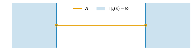
Figure 4: When $A$ is not closed, the set $\{x\in H\leavevmode\nobreak\ :\leavevmode\nobreak\ \Pi_{A}(x)=\emptyset\}$ has positive measure. For $\sigma$-quasioptimal metric projections with $\sigma>1$, this is a subset of $\mathrm{bdr}A$.

Lemma 5.1.

Let $A\subseteq H$ be non-empty and $\sigma>1$. Then for every $x\in H$ the $\sigma$-quasioptimal metric projection $\Pi_{A}(x;\sigma)$ satisfies

1. $\Pi_{A}(x;\sigma)=\{x\}$ when $x\in A$;

2. $\Pi_{A}(x;\sigma)\neq\emptyset$ when $x\in A\cup(H\setminus\overline{A})$;

3. $\Pi_{A}(x;\sigma)=\emptyset$ when $x\in\overline{A}\setminus A$.

Proof.

$\bm{1.}$ For $x\in A$, we have $\mathrm{dist}(x,A)=0$, and $|x-a|=0$ leads to $a=x$.

$\bm{2.}$ When $x\in H\setminus\overline{A}$, the distance is positive $\mathrm{dist}(x,A)>0$, and there exists a minimising sequence $(a_{n})\subset A$ such that $|x-a_{n}|\to\mathrm{dist}(x,A)$ from above. That is, for every $\varepsilon>0$ we can pick $N$ large enough so that $0\leq|x-a_{n}|-\mathrm{dist}(x,A)<\varepsilon$ for all $n\geq N$. If we choose $\varepsilon=(\sigma-1)\cdot\mathrm{dist}(x,A)>0$ then the tail of the sequence $(a_{n})$ belongs to $\Pi_{A}(x;\sigma)$.

$\bm{3.}$ Lastly, $\mathrm{dist}(x,A)=0$ for $x\in\overline{A}\setminus A$. For every $a\in\Pi_{A}(x;\sigma)$ this implies that $|x-a|=0$ and $x=a$, which contradicts the assumption that $x\not\in A$. ∎

Corollary 5.2.

Let $A\subseteq H$ be non-empty and $\sigma>1$.

1. Let $\mathcal{V}\subseteq H$ be a neighbourhood of $\hat{a}\in A$. The $\sigma$-quasioptimal metric projection $\Pi_{A}(x;\sigma)$ is non-empty for each $x\in\mathcal{V}$ if and only if $A\cap\mathcal{V}$ is closed in $\mathcal{V}$.

2. The $\sigma$-quasioptimal metric projection $\Pi_{A}(x;\sigma)$ is non-empty for every $x\in H$ if and only if $A$ is closed.

Proof.

Let $x\in\mathcal{V}$ be a limit point of $A\cap\mathcal{V}$, so that $\mathrm{dist}(x,A)=0$. If $\Pi_{A}(x;\sigma)\neq\emptyset$, there exists a point $a\in A$ such that $|x-a|\leq\sigma\cdot\mathrm{dist}(x,A)=0$ and thus $x=a\in A\cap\mathcal{V}$. In the other direction, if $A\cap\mathcal{V}$ is closed in $\mathcal{V}$ then every limit point of $A\cap\mathcal{V}$ in $\mathcal{V}$ belongs to $A$. Therefore, each $x\in\mathcal{V}$ either lies in $A$ or has $\mathrm{dist}(x,A)>0$, in which case we can repeat the argument from the proof of Lemma 5.1. For the second part, choose $\mathcal{V}=H$. ∎

Remark 5.3.

2. Lemma 5.1 and Corollary 5.2 hold in general Hilbert spaces.

3. When $\sigma=1$, the second part of Corollary 5.2 remains true in the Euclidean setting, but cannot be extended to the infinite-dimensional case. Indeed, there are closed sets in Hilbert spaces such that certain points have empty optimal metric projections onto them (see [5, Example 3.13]).

4. If $A\cap\mathcal{V}$ is closed in $\mathcal{V}$, the first part of Corollary 5.2 states that the $\sigma$-quasioptimal metric projection exists for every $x\in\mathcal{V}$ when $\sigma>1$. For optimal metric projections, this can be guaranteed only in a smaller neighbourhood (see Lemma 2.1).

5.2 Pythagorean property of super-regular sets

Until now, our discussion of quasioptimal metric projections was based only on the metric properties of the ambient space. At the same time, the Euclidean structure of $H$ makes it possible to compare the directions of optimal and quasioptimal metric projections.

Consider a hyperplance $A$, a point $x\not\in A$, its orthogonal projection $\pi\in A$ and a quasioptimal metric projection $\pi_{\sigma}\in\Pi_{A}(x;\sigma)$. A basic trigonometric argument gives that $\pi-x$ and $\pi_{\sigma}-x$ form an acute angle that is upper bounded by $\arccos(\frac{1}{\sigma})$. Thus, the quasioptimal metric projections onto a hyperplance enjoy a geometric property that we call Pythagorean: they are aligned with the direction of the optimal metric projection. See Fig. 5 for a two-dimensional example.

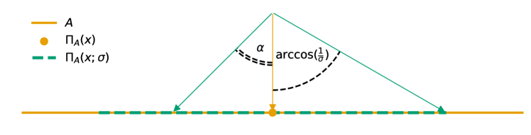
Figure 5: Every $\sigma$-quasioptimal projection onto a hyperplane satisfies the Pythagorean property: the angle $\alpha$ it forms with the orthogonal projection is bounded by $\arccos(\frac{1}{\sigma})$.

In Lemma 5.4 and Corollary 5.5, we show that the Pythagorean property persists as we substitute the hyperplane for a super-regular set. This intuitive result allows us to prove that the alternating projections with two quasioptimal projections converge (Theorem 6.6). In Appendix A, we derive analogues of Lemma 5.4 for prox-regular and convex sets.

Lemma 5.4.

Let $A\subseteq H$ be non-empty and super-regular at $\hat{a}\in A$. Then for every $\varepsilon>0$ there exists $\delta>0$ such that for every $x\in{{\mathbb{B}}}_{\delta/2}(\hat{a})\setminus A$ it holds that

$$\bigg{\langle}\frac{x-\pi}{|x-\pi|},\frac{x-a}{|x-a|}\bigg{\rangle}\geq\frac{|x-\pi|}{|x-a|}-\varepsilon(1+\varepsilon)$$

for each $\pi\in\Pi_{A}(x)$ and $a\in A\cap{{\mathbb{B}}}_{\delta}(\hat{a})$.

Proof.

Fix $\varepsilon>0$. Since $A$ is super-regular at $\hat{a}$, we can choose $\delta>0$ such that $A\cap{{\mathbb{B}}}_{\delta}(\hat{a})$ is closed in ${{\mathbb{B}}}_{\delta}(\hat{a})$ and property (5) holds:

$$\langle v,a^{\prime}-a\rangle\leq\varepsilon|v|\cdot|a^{\prime}-a|\quad\text{for all}\quad a,a^{\prime}\in A\cap{{\mathbb{B}}}_{\delta}(\hat{a})\quad\text{and}\quad v\in N^{\mathrm{lim}}_{A}(a).$$

For each $x\in{{\mathbb{B}}}_{\delta/2}(\hat{a})$, Lemma 2.1 states that the optimal metric projection $\Pi_{A}(x)$ is non-empty and every $\pi\in\Pi_{A}(x)$ lies in $A\cap{{\mathbb{B}}}_{\delta}(\hat{a})$.

Pick $\pi\in\Pi_{A}(x)$, $a\in A\cap{{\mathbb{B}}}_{\delta}(\hat{a})$, and recall that $x-\pi\in N^{\mathrm{lim}}_{A}(\pi)$. By property (5),

$$\varepsilon|x-\pi|\cdot|a-\pi|\geq\langle x-\pi,a-\pi\rangle=|x-\pi|^{2}-\langle x-\pi,x-a\rangle.$$

Lemma 2.2 gives $|\pi-a|\leq(1+\varepsilon)|x-a|$, and we conclude that

$$\langle x-\pi,x-a\rangle\geq|x-\pi|\big{(}|x-\pi|-\varepsilon|a-\pi|\big{)}\geq|x-\pi|\big{(}|x-\pi|-\varepsilon(1+\varepsilon)|x-a|\big{)}.\qed$$

Corollary 5.5.

Let $A\subseteq H$ be non-empty and super-regular at $\hat{a}\in A$. Then for every $\varepsilon>0$ there exists $\delta>0$ such that for every $x\in{{\mathbb{B}}}_{\delta/2}(\hat{a})\setminus A$ it holds that

$$\bigg{\langle}\frac{x-\pi}{|x-\pi|},\frac{x-\pi_{\sigma}}{|x-\pi_{\sigma}|}\bigg{\rangle}\geq\frac{1}{\sigma}-\varepsilon(1+\varepsilon)$$

for each $\pi\in\Pi_{A}(x)$ and $\pi_{\sigma}\in\Pi_{A}(x;\sigma)\cap{{\mathbb{B}}}_{\delta}(\hat{a})$.

Remark 5.6.

The Pythagorean property can be violated when the set is not super-regular (see Fig. 6). Fix a positive constant $d>0$ and consider a closed piecewise linear curve $A\subset\mathbb{R}^{2}$ with vertices $a_{n}$ defined for every $n\in\mathbb{Z}$ as $a_{0}=(0,0)$ and

$$a_{n+1}=a_{n}+2^{-n}d\cdot\begin{cases}(0,-1),&n\pmod{4}\equiv 0,\\ (1,0),&n\pmod{4}\equiv 1,\\ (0,1),&n\pmod{4}\equiv 2,\\ (-1,0),&n\pmod{4}\equiv 3.\end{cases}$$

Simple series summation gives $a_{n}\to\hat{a}=\frac{2}{5}(d,-2d)$ as $n\to\infty$. For every $k\in\mathbb{Z}$,

$$a_{4k}=\frac{2}{5}\left[1-2^{-4k}\right](d,-2d),\quad a_{4k-1}=a_{4k}+2^{-4k}(2d,0).$$

Therefore, every linear segment $[a_{4k},a_{4k-1}]$ is horizontal, and the vertical line through $\hat{a}$ intersects each of them. Consider a sequence of points $(x_{k})$ defined by

$$x_{k}=\frac{2}{5}\left(d,-2\left[1-\frac{17}{32}\cdot 2^{-4k}\right]d\right),\quad k\in\mathbb{Z}.$$

Each $x_{k}$ has the same first coordinate as $\hat{a}$ and is equidistant from the horizontal segments $[a_{4k},a_{4k-1}]$ and $[a_{4k+4},a_{4k+3}]$ with $\mathrm{dist}(x_{k},A)=\frac{3}{8}\cdot 2^{-4k}d$. The optimal metric projection of $x_{k}$ onto $A$ consists of two points $\Pi_{A}(x_{k})=\{\pi_{k,1},\pi_{k,2}\}$, where

$$\pi_{k,1}=\frac{2}{5}\left(d,-2\left[1-2^{-4k}\right]d\right),\quad\pi_{k,2}=\frac{2}{5}\left(d,-2\left[1-\frac{1}{16}\cdot 2^{-4k}\right]d\right),$$

which are oriented in opposite directions

$$\bigg{\langle}\frac{x_{k}-\pi_{k,1}}{|x_{k}-\pi_{k,1}|},\frac{x_{k}-\pi_{k,2}}{|x_{k}-\pi_{k,2}|}\bigg{\rangle}=-1.$$

Thus, since $x_{k}\to\hat{a}$ as $k\to\infty$, every neighbourhood of $\hat{a}$ contains a point, whose optimal metric projections onto $A$ violate the Pythagorean property.

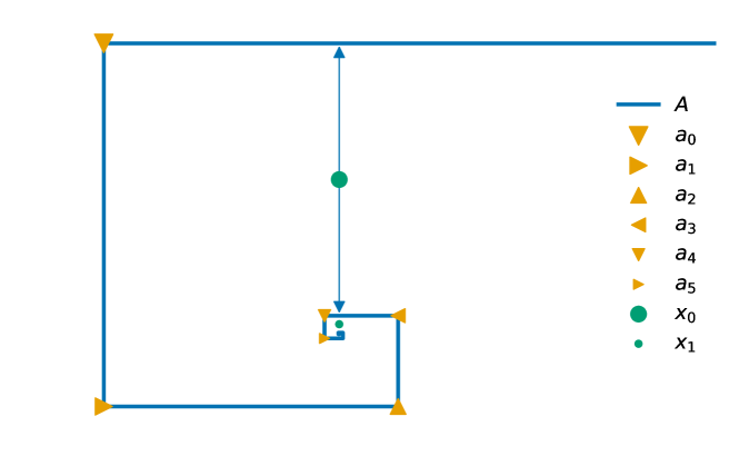
Figure 6: The Pythagorean property can be violated when $A$ is not super-regular.

The Pythagorean property also gives us better control over the location of $\Pi_{A}(x;\sigma)$ relative to $\Pi_{A}(x)$. Recall a simple bound $|\pi_{\sigma}-\pi|\leq(\sigma+1)\cdot\mathrm{dist}(x,A)$ that holds for every $\pi_{\sigma}\in\Pi_{A}(x;\sigma)$ and $\pi\in\Pi_{A}(x)$. This estimate turns out to be rather pessimistic for super-regular sets, especially when $\sigma$ is close to 1.

Corollary 5.7.

Let $A\subseteq H$ be non-empty and super-regular at $\hat{a}\in A$. Then for every $\varepsilon>0$ there exists $\delta>0$ such that for every $x\in{{\mathbb{B}}}_{\delta/2}(\hat{a})$ and every $\sigma\geq 1$ it holds that

$$|\pi_{\sigma}-\pi|\leq\left(\varepsilon+\sqrt{\sigma^{2}-1+\varepsilon^{2}}\right)\cdot\mathrm{dist}(x,A)$$

for each $\pi\in\Pi_{A}(x)$ and $\pi_{\sigma}\in\Pi_{A}(x;\sigma)\cap{{\mathbb{B}}}_{\delta}(\hat{a})$.

Proof.

From the proof of Lemma 5.4, we get

$$\langle x-\pi,x-\pi_{\sigma}\rangle\geq|x-\pi|\big{(}|x-\pi|-\varepsilon|\pi_{\sigma}-\pi|\big{)}.$$

We put this estimate into the following expression of the squared norm

$$|\pi_{\sigma}-\pi|^{2} =|\pi-x|^{2}+|\pi_{\sigma}-x|^{2}-2\langle x-\pi,x-\pi_{\sigma}\rangle$$

$$\leq(\sigma^{2}-1)|\pi-x|^{2}+2\varepsilon|\pi-x||\pi_{\sigma}-\pi|.$$

It remains to solve the inequality for $|\pi_{\sigma}-\pi|$ and note that $|\pi-x|=\mathrm{dist}(x,A)$. ∎

6 Convergence of quasioptimal alternating projections

6.1 Technical convergence lemma

We begin to study the convergence of quasioptimal alternating projections (3). The techniques we use are inspired by [66]. Broadly speaking, we will approach the proof of convergence by showing that the steps taken by the method ($|b_{n+1}-a_{n}|$ and $|a_{n+1}-b_{n+1}|$) shrink with iterations.

We will consider three separate scenarios, which differ in the values taken by the quasioptimality constants $\sigma_{A}$ and $\sigma_{B}$ and the properties that we ask from the sets $A$ and $B$. These nuances lead to different estimates on the step sizes. The proofs of convergence, however, follow the same pattern, which we summarise in Lemma 6.1.

Lemma 6.1.

Let $A,B\subseteq H$ be non-empty and assume that there is an open set $\mathcal{V}\subseteq H$ such that $A\cap\mathcal{V}$ and $B\cap\mathcal{V}$ are closed in $\mathcal{V}$. Let $\mathcal{U}\subset\mathcal{V}$ be closed and $\kappa_{A},\kappa_{B}>0$. Suppose that, for $n\geq 1$, sequences $(a_{n})\subset A\cap\mathcal{U}$ and $(b_{n})\subset B\cap\mathcal{U}$ satisfy

$$|a_{n}-b_{n}|\leq\kappa_{A}|b_{n}-a_{n-1}|,\quad|b_{n+1}-a_{n}|\leq\kappa_{B}|a_{n}-b_{n}|.$$

If $\kappa_{A}\cdot\kappa_{B}<1$ then $(a_{n})$ and $(b_{n})$ converge to a common limit $\hat{x}\in A\cap B\cap\mathcal{U}$ and, for $n\geq 0$,

$$|\hat{x}-a_{n}|\leq\tfrac{1+\kappa_{A}}{1-\kappa_{A}\kappa_{B}}(\kappa_{A}\kappa_{B})^{n}\cdot|b_{1}-a_{0}|,\quad|\hat{x}-b_{n+1}|\leq\tfrac{(1+\kappa_{B})\kappa_{A}}{1-\kappa_{A}\kappa_{B}}(\kappa_{A}\kappa_{B})^{n}\cdot|b_{1}-a_{0}|.$$

Proof.

By induction, we get that for all $n\geq 0$ the sequences $(a_{n})$ and $(b_{n})$ satisfy

$$|b_{n+1}-a_{n}|\leq(\kappa_{A}\kappa_{B})^{n}\cdot|b_{1}-a_{0}|,\quad|a_{n+1}-b_{n+1}|\leq\kappa_{A}(\kappa_{A}\kappa_{B})^{n}\cdot|b_{1}-a_{0}|.$$

Next, we show that the sequence $(a_{0},b_{1},a_{1},b_{2},a_{2},\ldots)$ is Cauchy. To this end, fix an arbitrary $n>0$; then for every $k>n$ we have

$$\max\{|a_{k}-a_{n}|,|b_{k}-a_{n}|\} \leq|b_{n+1}-a_{n}|+|a_{n+1}-b_{n+1}|+|b_{n+2}-a_{n+1}|+\ldots$$

$$\leq|b_{1}-a_{0}|\cdot\left[(\kappa_{A}\kappa_{B})^{n}+\kappa_{A}(\kappa_{A}\kappa_{B})^{n}+(\kappa_{A}\kappa_{B})^{n+1}+\ldots\right]$$

$$=\tfrac{1+\kappa_{A}}{1-\kappa_{A}\kappa_{B}}(\kappa_{A}\kappa_{B})^{n}\cdot|b_{1}-a_{0}|,$$

and for every $k\geq n$ it holds that

$$\max\{|a_{k}-b_{n}|,|b_{k}-b_{n}|\} \leq|a_{n}-b_{n}|+|b_{n+1}-a_{n}|+|a_{n+1}-b_{n+1}|+\ldots$$

$$\leq|b_{1}-a_{0}|\cdot\left[\kappa_{A}(\kappa_{A}\kappa_{B})^{n-1}+(\kappa_{A}\kappa_{B})^{n}+\kappa_{A}(\kappa_{A}\kappa_{B})^{n}+\ldots\right]$$

$$=\tfrac{(1+\kappa_{B})\kappa_{A}}{1-\kappa_{A}\kappa_{B}}(\kappa_{A}\kappa_{B})^{n-1}\cdot|b_{1}-a_{0}|.$$

Therefore, the sequence is indeed Cauchy and has a limit $\hat{x}$, which satisfies

$$|\hat{x}-a_{n}|\leq\tfrac{1+\kappa_{A}}{1-\kappa_{A}\kappa_{B}}(\kappa_{A}\kappa_{B})^{n}\cdot|b_{1}-a_{0}|,\quad|\hat{x}-b_{n+1}|\leq\tfrac{(1+\kappa_{B})\kappa_{A}}{1-\kappa_{A}\kappa_{B}}(\kappa_{A}\kappa_{B})^{n}\cdot|b_{1}-a_{0}|.$$

Moreover, $\hat{x}$ is a limit point of both $A\cap\mathcal{U}$ and $B\cap\mathcal{U}$, which are closed in $\mathcal{V}$. So $\hat{x}\in A\cap B\cap\mathcal{U}$. ∎

6.2 One projection is quasioptimal

In this section we assume that the projection onto $B$ is optimal. The projection onto $A$ is allowed to be quasioptimal, and we specify that $A$ is super-regular. It is only natural to couple the quasioptimality of the projection with the super-regularity of the set, given the appealing properties that they possess when considered together (see Lemma 5.4 and Corollary 5.7).

The following lemma adapts a sub-result of [66, Theorem 5.2] to the case of quasioptimal projections. It will allow us to estimate the step $|a_{n+1}-b_{n+1}|$ in terms of its predecessor $|b_{n+1}-a_{n}|$ in the proof of the convergence Theorem 6.3. In Corollary 6.4, we obtain a faster convergence rate when $B$ is super-regular too. We illustrate the settings of Lemma 6.2 in Fig 7.

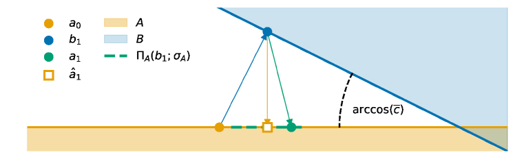
Figure 7: The illustration of the settings of Lemma 6.2.

Lemma 6.2.

Let non-empty sets $A,B\subseteq H$ have a common point $\overline{x}\in A\cap B$, where

• $A$ and $B$ are locally closed and intersect transversally with $\cos(A,B,\overline{x})=\overline{c}<1$, and

• $A$ is super-regular.

Pick $\varepsilon>0$ and $c\in(\overline{c},1)$. There exists $\delta>0$ such that for every $\sigma_{A}\geq 1$, each triplet of points $a_{0}\in A\cap{{\mathbb{B}}}_{\delta}(\overline{x})$, $b_{1}\in\Pi_{B}(a_{0})\cap{{\mathbb{B}}}_{\delta}(\overline{x})$ with $\Pi_{A}(b_{1})\cap{{\mathbb{B}}}_{\delta}(\overline{x})\neq\emptyset$, and $a_{1}\in\Pi_{A}(b_{1};\sigma_{A})$ satisfies

$$|a_{1}-b_{1}|\leq\sigma_{A}(c+2\varepsilon)\cdot|b_{1}-a_{0}|.$$

If $a_{0}\in A$ is such that $|a_{0}-\overline{x}|<\tfrac{\delta}{4}$ then $b_{1}$ and $a_{1}$ are well-defined, and the estimate holds for every $b_{1}\in\Pi_{B}(a_{0})$.

Proof.

Fix $\varepsilon$ and $c$. First, we set $\delta=\min\{\delta_{1}(\varepsilon),\delta_{2},\delta_{3}(c)\}$, where $\delta_{1}(\varepsilon)$ comes from the definition of super-regularity for $A$; $\delta_{2}$ ensures that $B\cap{{\mathbb{B}}}_{\delta_{2}}(\overline{x})$ is closed in ${{\mathbb{B}}}_{\delta_{2}}(\overline{x})$; and $\delta_{3}(c)$ ensures that the assertion of Lemma 2.4 holds in ${{\mathbb{B}}}_{\delta_{3}(c)}(\overline{x})$.

Consider $\hat{a}_{1}\in\Pi_{A}(b_{1})\cap{{\mathbb{B}}}_{\delta}(\overline{x})$. Then $|a_{1}-b_{1}|\leq\sigma_{A}\cdot|\hat{a}_{1}-b_{1}|$ and it remains to estimate $|\hat{a}_{1}-b_{1}|$ in terms of $|b_{1}-a_{0}|$. If either of them is zero, the proof is complete. Otherwise, we expand the squared norm

$$|\hat{a}_{1}-b_{1}|^{2}=\langle b_{1}-\hat{a}_{1},a_{0}-\hat{a}_{1}\rangle+\langle\hat{a}_{1}-b_{1},a_{0}-b_{1}\rangle.$$

Recall that $A$ is super-regular at $\overline{x}$. Since $a_{0},\hat{a}_{1}\in A\cap{{\mathbb{B}}}_{\delta}(\overline{x})$ and $b_{1}-\hat{a}_{1}\in N^{\mathrm{lim}}_{A}(\hat{a}_{1})$, we have

$$\langle b_{1}-\hat{a}_{1},a_{0}-\hat{a}_{1}\rangle\leq\varepsilon|b_{1}-\hat{a}_{1}|\cdot|a_{0}-\hat{a}_{1}|\leq 2\varepsilon|b_{1}-\hat{a}_{1}|\cdot|a_{0}-b_{1}|.$$

In addition, $a_{0}-b_{1}\in N^{\mathrm{lim}}_{B}(b_{1})$ and $b_{1}\in B\cap{{\mathbb{B}}}_{\delta}(\overline{x})$. Thanks to transversality and Lemma 2.4,

$$\langle\hat{a}_{1}-b_{1},a_{0}-b_{1}\rangle\leq c|\hat{a}_{1}-b_{1}|\cdot|a_{0}-b_{1}|.$$

Adding the two estimates, we get $|\hat{a}_{1}-b_{1}|\leq(c+2\varepsilon)\cdot|a_{0}-b_{1}|$.

Finally, we show that the points $b_{1}$ and $a_{1}$ are well-defined when $a_{0}\in A\cap{{\mathbb{B}}}_{\delta/4}(\overline{x})$. By Lemma 2.1, the optimal metric projection $\Pi_{B}(a_{0})$ is non-empty and $|b_{1}-\overline{x}|\leq 2|a_{0}-\overline{x}|<\delta/2$. We can use Lemma 2.1 again to show that $\emptyset\neq\Pi_{A}(b_{1})\subseteq\Pi_{A}(b_{1};\sigma_{A})$ and $\Pi_{A}(b_{1})\subseteq{{\mathbb{B}}}_{\delta}(\overline{x})$. ∎

Theorem 6.3.

Let non-empty sets $A,B\subseteq H$ have a common point $\overline{x}\in A\cap B$, where

• $A$ and $B$ are locally closed and intersect transversally with $\cos(A,B,\overline{x})=\overline{c}<1$, and

• $A$ is super-regular.

For every $c\in(\overline{c},1)$ there exists $\delta>0$ such that for every $\sigma_{A}\geq 1$ satisfying $\kappa=\sigma_{A}\cdot c<1$ and every $a_{0}\in A$ satisfying $|a_{0}-\overline{x}|<\frac{1-\kappa}{8}\delta$, the quasioptimal alternating projections (3) with $\sigma_{B}=1$ converge to $\hat{x}\in A\cap B$ such that $|\hat{x}-\overline{x}|<\tfrac{3}{8}\delta$ and, for $n\geq 0$,

$$|\hat{x}-a_{n}|\leq\tfrac{1+\kappa}{1-\kappa}\kappa^{n}\cdot\mathrm{dist}(a_{0},B),\quad|\hat{x}-b_{n+1}|\leq\tfrac{2\kappa}{1-\kappa}\kappa^{n}\cdot\mathrm{dist}(a_{0},B).$$

Proof.

Fix $c$ and choose $\delta$ as follows: pick some $c^{\prime}\in(\overline{c},c)$, set $\varepsilon=\frac{1}{2}(c^{\prime}-c)$ and use the value of $\delta$ from Lemma 6.2 that corresponds to $c^{\prime}$ and $\varepsilon$. This gives $\sigma_{A}(c^{\prime}+2\varepsilon)=\kappa<1$.

Let us assume for a moment that the sequences $(a_{n})$ and $(b_{n})$ are well-defined and that $|a_{n}-\overline{x}|<\delta/4$ for all $n\geq 0$. Then Lemma 6.2 and the definition of $\Pi_{B}(a_{n})$ guarantee that

$$|a_{n}-b_{n}|\leq\kappa|b_{n}-a_{n-1}|,\quad|b_{n+1}-a_{n}|\leq|a_{n}-b_{n}|,\quad n\geq 1.$$

In addition, for every $n\geq 1$ we have

$$|b_{n}-\overline{x}|\leq|b_{n}-a_{n-1}|+|a_{n-1}-\overline{x}|<|b_{1}-a_{0}|+|a_{n-1}-\overline{x}|<\tfrac{3-\kappa}{8}\delta=\tilde{\delta}.$$

This means that we can apply the convergence Lemma 6.1: setting $\mathcal{V}={{\mathbb{B}}}_{\delta}(\overline{x})$, $\mathcal{U}=\overline{{{\mathbb{B}}}_{\tilde{\delta}}(\overline{x})}$, $\kappa_{A}=\kappa$ and $\kappa_{B}=1$, we get the convergence to a point $\hat{x}\in A\cap B\cap\mathcal{U}$ at a rate

$$|\hat{x}-a_{n}|\leq\tfrac{1+\kappa}{1-\kappa}\kappa^{n}\cdot|b_{1}-a_{0}|,\quad|\hat{x}-b_{n+1}|\leq\tfrac{2\kappa}{1-\kappa}\kappa^{n}\cdot|b_{1}-a_{0}|,\quad n\geq 0.$$

It remains to note that $|b_{1}-a_{0}|=\mathrm{dist}(a_{0},B)$.

Now we prove that our assumptions are satisfied. Let $n=0$ and $d_{0}=|a_{0}-\overline{x}|<\frac{1-\kappa}{8}\delta$. As $d_{0}<\delta/4$, Lemma 6.2 states that $b_{1}$ and $a_{1}$ exist and $|a_{1}-b_{1}|\leq\kappa|b_{1}-a_{0}|$. Moreover,

$$|a_{1}-\overline{x}| \leq|a_{1}-b_{1}|+|b_{1}-a_{0}|+|a_{0}-\overline{x}|$$

$$\leq(2+\kappa)d_{0}=\tfrac{d_{0}}{1-\kappa}\left[2-\kappa(1+\kappa)\right]<\delta/4.$$

Suppose that the sequences are well-defined up until $b_{n}$ and $a_{n}$, and that

$$|a_{n}-\overline{x}|\leq\tfrac{d_{0}}{1-\kappa}\left[2-\kappa^{n}(1+\kappa)\right].$$

Then $|a_{n}-\overline{x}|<\delta/4$, and we can use Lemma 6.2 again to show that $b_{n+1}$ and $a_{n+1}$ exist and satisfy $|a_{n+1}-b_{n+1}|\leq\kappa|b_{n+1}-a_{n}|$. This leads to

$$|a_{n+1}-\overline{x}| \leq|a_{n+1}-b_{n+1}|+|b_{n+1}-a_{n}|+|a_{n}-\overline{x}|$$

$$\leq(1+\kappa)\kappa^{n}d_{0}+\tfrac{d_{0}}{1-\kappa}\left[2-\kappa^{n}(1+\kappa)\right]$$

$$=\tfrac{d_{0}}{1-\kappa}\left[2-\kappa^{n+1}(1+\kappa)\right]<\delta/4.$$

It follows that $(a_{n})$ and $(b_{n})$ are well-defined and $(a_{n})\subset{{\mathbb{B}}}_{\delta/4}(\overline{x})$, which finishes the proof. ∎

Corollary 6.4.

Let non-empty sets $A,B\subseteq H$ have a common point $\overline{x}\in A\cap B$, where

• $A$ and $B$ are locally closed and intersect transversally with $\cos(A,B,\overline{x})=\overline{c}<1$, and

• $A$ and $B$ are super-regular.

For every $c\in(\overline{c},1)$ there exists $\delta>0$ such that for every $\sigma_{A}\geq 1$ satisfying $c\kappa<1$ with $\kappa=\sigma_{A}\cdot c$ and every $a_{0}\in A$ satisfying $|a_{0}-\overline{x}|<\frac{1-c\kappa}{4[2+\kappa(1-c)]}\delta$, the quasioptimal alternating projections (3) with $\sigma_{B}=1$ converge to $\hat{x}\in A\cap B$ such that $|\hat{x}-\overline{x}|<\tfrac{3}{8}\delta$ and, for $n\geq 0$,

$$|\hat{x}-a_{n}|\leq\tfrac{1+\kappa}{1-c\kappa}(c\kappa)^{n}\cdot\mathrm{dist}(a_{0},B),\quad|\hat{x}-b_{n+1}|\leq\tfrac{(1+c)\kappa}{1-c\kappa}(c\kappa)^{n}\cdot\mathrm{dist}(a_{0},B).$$

Proof.

The proof mimics that of Theorem 6.3, so we only highlight the differences. We need to make sure that the results of Lemma 6.2 can be applied to both $A$ and $B$. Therefore, we choose $c^{\prime}$ and $\varepsilon$ as in Theorem 6.3 and set $\delta=\min\{\delta_{A},\delta_{B}\}$, where $\delta_{A}$ and $\delta_{B}$ come from Lemma 6.2 for $A$ and $B$, respectively. It follows that

$$|a_{n}-b_{n}|\leq\kappa|b_{n}-a_{n-1}|,\quad|b_{n+1}-a_{n}|\leq c|a_{n}-b_{n}|,\quad n\geq 1,$$

provided that the sequences are well-defined and $(a_{n})\subset{{\mathbb{B}}}_{\delta/4}(\overline{x})$. This can be shown by a modified induction argument, where we prove that

$$|a_{n}-\overline{x}|\leq\tfrac{|a_{0}-\overline{x}|}{1-c\kappa}\left[2+\kappa(1-c)-(c\kappa)^{n}(1+\kappa)\right]<\delta/4.\qed$$

6.3 Both projections are quasioptimal

Now, we even out the assumptions related to $A$ and $B$. We suppose that both sets are super-regular and consider quasioptimal metric projections with $\sigma_{A}>1$ and $\sigma_{B}>1$. In Lemma 6.5 we estimate the length of the steps taken by the method of quasioptimal alternating projections (see Fig. 8). This result relies on the Pythagorean property for $B$ (unlike the previous Lemma 6.2) and leads to our second convergence Theorem 6.6.

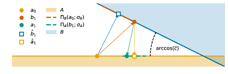
Figure 8: The illustration of the settings of Lemma 6.5.

Lemma 6.5.

Let non-empty sets $A,B\subseteq H$ have a common point $\overline{x}\in A\cap B$, where

• $A$ and $B$ are locally closed and intersect transversally with $\cos(A,B,\overline{x})=\overline{c}<1$, and

• $A$ and $B$ are super-regular.

Pick $\varepsilon>0$ and $c\in(\overline{c},1)$. There exists $\delta>0$ such that for every $\sigma_{A}\geq 1$ and $\sigma_{B}\geq 1$, each triplet of points $a_{0}\in A\cap{{\mathbb{B}}}_{\delta}(\overline{x})$ with $\Pi_{B}(a_{0})\cap{{\mathbb{B}}}_{\delta}(\overline{x})\neq\emptyset$, $b_{1}\in\Pi_{B}(a_{0};\sigma_{B})\cap{{\mathbb{B}}}_{\delta}(\overline{x})$ with $\Pi_{A}(b_{1})\cap{{\mathbb{B}}}_{\delta}(\overline{x})\neq\emptyset$, and $a_{1}\in\Pi_{A}(b_{1};\sigma_{A})$ satisfies

$$|a_{1}-b_{1}|\leq\sigma_{A}f(\varepsilon,c,\sigma_{B})\cdot|b_{1}-a_{0}|,$$

where

$$f(\varepsilon,c,\sigma_{B})=2\varepsilon+c\left(\tfrac{1}{\sigma_{B}}-\varepsilon(1+\varepsilon)\right)+\sqrt{1-c^{2}}\sqrt{1-\left(\tfrac{1}{\sigma_{B}}-\varepsilon(1+\varepsilon)\right)^{2}}.$$

If $a_{0}\in A$ is such that $|a_{0}-\overline{x}|<\tfrac{\delta}{2(\sigma_{B}+1)}$ then $b_{1}$ and $a_{1}$ are well-defined, and the estimate holds for every $b_{1}\in\Pi_{B}(a_{0})$.

Proof.

For fixed $\varepsilon$ and $c$, we select $\delta$ just as in Corollary 6.4 to ensure that super-regular properties of $A$ and $B$ together with Lemma 2.4 hold in ${{\mathbb{B}}}_{\delta}(\overline{x})$. We then follow the proof of Lemma 6.2 with some modifications. If $a_{1}=b_{1}$ or $b_{1}=a_{0}$ then the proof is complete. Otherwise, take an optimal metric projection $\hat{a}_{1}\in\Pi_{A}(b_{1})\cap{{\mathbb{B}}}_{\delta}(\overline{x})$, get the inequality $|a_{1}-b_{1}|\leq\sigma_{A}\cdot|\hat{a}_{1}-b_{1}|$ and expand the squared norm

$$|\hat{a}_{1}-b_{1}|^{2}=\langle b_{1}-\hat{a}_{1},a_{0}-\hat{a}_{1}\rangle+\langle\hat{a}_{1}-b_{1},a_{0}-b_{1}\rangle.$$

The first term is bounded like in Lemma 6.2 based on the super-regularity of $A$:

$$\langle b_{1}-\hat{a}_{1},a_{0}-\hat{a}_{1}\rangle\leq 2\varepsilon|b_{1}-\hat{a}_{1}|\cdot|a_{0}-b_{1}|.$$

In the second term, however, we can no longer guarantee that $a_{0}-b_{1}\in N^{\mathrm{lim}}_{B}(b_{1})$ since $b_{1}$ is a quasioptimal projection. Let $\hat{b}_{1}\in\Pi_{B}(a_{0})\cap{{\mathbb{B}}}_{\delta}(\overline{x})$; then by Lemma 2.4,

$$\langle\hat{a}_{1}-b_{1},a_{0}-\hat{b}_{1}\rangle\leq c|\hat{a}_{1}-b_{1}|\cdot|a_{0}-\hat{b}_{1}|,$$

since $\hat{a}_{1}\neq\hat{b}_{1}$ and $a_{0}\neq\hat{b}_{1}$. By virtue of Lemma 5.4, we have

$$\langle a_{0}-b_{1},a_{0}-\hat{b}_{1}\rangle\geq\left(\tfrac{1}{\sigma_{B}}-\varepsilon(1+\varepsilon)\right)|a_{0}-b_{1}||a_{0}-\hat{b}_{1}|.$$

Consider three angles: $\alpha$ between $\hat{a}_{1}-b_{1}$ and $a_{0}-\hat{b}_{1}$, $\beta$ between $a_{0}-b_{1}$ and $a_{0}-\hat{b}_{1}$, and $\gamma$ between $\hat{a}_{1}-b_{1}$ and $a_{0}-b_{1}$. The triangle inequality on the sphere gives $\gamma\geq\alpha-\beta$, so that

$$\cos(\gamma)\leq\cos(\alpha-\beta)\leq\cos\left(\arccos(c)-\arccos\left(\tfrac{1}{\sigma_{B}}-\varepsilon(1+\varepsilon)\right)\right)$$

and

$$\langle\hat{a}_{1}-b_{1},a_{0}-b_{1}\rangle\leq(f(c,\varepsilon,\sigma_{B})-2\varepsilon)\cdot|b_{1}-\hat{a}_{1}||a_{0}-b_{1}|.$$

Let us show that the points $b_{1}$ and $a_{1}$ are well-defined when $|a_{0}-\overline{x}|<\tfrac{\delta}{2(\sigma_{B}+1)}$. By Lemma 2.1, $\Pi_{B}(a_{0};\sigma_{B})\neq\emptyset$ for all $\sigma_{B}\geq 1$ and $|b_{1}-\overline{x}|<\delta/2$ for every $b_{1}\in\Pi_{B}(a_{0};\sigma_{B})$. Then Lemma 2.1 gives that $\Pi_{A}(b_{1};\sigma_{A})\neq\emptyset$ for all $\sigma_{A}\geq 1$ and $\Pi_{A}(b_{1})\subseteq{{\mathbb{B}}}_{\delta}(\overline{x})$. ∎

Theorem 6.6.

Let non-empty sets $A,B\subseteq H$ have a common point $\overline{x}\in A\cap B$, where

• $A$ and $B$ are locally closed and intersect transversally with $\cos(A,B,\overline{x})=\overline{c}<1$, and

• $A$ and $B$ are super-regular.

For every $c\in(\overline{c},1)$ and every $\sigma_{A},\sigma_{B}\in(1,\frac{1}{c})$ define $\kappa_{A}$ and $\kappa_{B}$ as

$$\kappa_{A}=\frac{\sigma_{A}}{\sigma_{B}}\left[c+\sqrt{1-c^{2}}\sqrt{\sigma_{B}^{2}-1}\right],\quad\kappa_{B}=\frac{\sigma_{B}}{\sigma_{A}}\left[c+\sqrt{1-c^{2}}\sqrt{\sigma_{A}^{2}-1}\right].$$

If $\kappa_{A}\cdot\kappa_{B}<1$ then there exists $\delta>0$ such that for every $a_{0}\in A$ satisfying

$$|a_{0}-\overline{x}|<\tfrac{1-\kappa_{A}\kappa_{B}}{2(\sigma_{B}+1)[\sigma_{B}+1+\kappa_{A}(\sigma_{B}-\kappa_{B})]}\delta,$$

the quasioptimal alternating projections (3) converge to $\hat{x}\in A\cap B$ such that $|\hat{x}-\overline{x}|<\tfrac{3}{8}\delta$ and, for $n\geq 0$,

$$|\hat{x}-a_{n}|\leq\tfrac{\sigma_{B}(1+\kappa_{A})}{1-\kappa_{A}\kappa_{B}}(\kappa_{A}\kappa_{B})^{n}\cdot\mathrm{dist}(a_{0},B),\quad|\hat{x}-b_{n+1}|\leq\tfrac{\sigma_{B}(1+\kappa_{B})\kappa_{A}}{1-\kappa_{A}\kappa_{B}}(\kappa_{A}\kappa_{B})^{n}\cdot\mathrm{dist}(a_{0},B).$$

Proof.

Similar to Theorem 6.3, we want to choose $c^{\prime}\in(\overline{c},c)$, pick some $\varepsilon>0$ and infer the corresponding value of $\delta$. Since the scaling factor in Lemma 6.5 is more complicated than in Lemma 6.2, the implicit function theorem is required. We only outline the argument here, and the details can be found in Appendix B.

The function $f$ from Lemma 6.5 satisfies $f(0,c,\sigma_{A})=\frac{\kappa_{B}}{\sigma_{B}}$ and $f(0,c,\sigma_{B})=\frac{\kappa_{A}}{\sigma_{A}}$. Provided that $c^{\prime}$ is sufficiently close to $c$, the implicit function theorem guarantees that we can find $\varepsilon_{A}$ and $\varepsilon_{B}$ such that $f(\varepsilon_{B},c^{\prime},\sigma_{A})=\frac{\kappa_{B}}{\sigma_{B}}$ and $f(\varepsilon_{A},c^{\prime},\sigma_{B})=\frac{\kappa_{A}}{\sigma_{A}}$. In addition, $\varepsilon_{A}$ and $\varepsilon_{B}$ are positive when $\sigma_{A}<1/c$ and $\sigma_{B}<1/c$, which is assumed.

We can then take $\varepsilon_{A}$ and choose $\delta_{A}>0$ based on Lemma 6.5. On reversing the roles of $A$ and $B$ in Lemma 6.5, we also get $\delta_{B}>0$ that corresponds to $\varepsilon_{B}$. Finally, we set $\delta=\min\{\delta_{A},\delta_{B}\}$. The rest is similar to the proof of Theorem 6.3. Thanks to Lemma 6.5, the steps satisfy

$$|a_{n}-b_{n}|\leq\kappa_{A}|b_{n}-a_{n-1}|,\quad|b_{n+1}-a_{n}|\leq\kappa_{B}|a_{n}-b_{n}|,\quad n\geq 1,$$

when $|a_{n}-\overline{x}|<\tfrac{\delta}{2(\sigma_{B}+1)}$. This, in turn, follows from an inductive proof of

$$|a_{n}-\overline{x}|\leq\tfrac{|a_{0}-\overline{x}|}{1-\kappa_{A}\kappa_{B}}\left[1+\sigma_{B}+\kappa_{A}(\sigma_{B}-\kappa_{B})-\sigma_{B}(\kappa_{A}\kappa_{B})^{n}(1+\kappa_{A})\right].$$

We should also note that $|b_{1}-a_{0}|\leq\sigma_{B}\cdot\mathrm{dist}(a_{0},B)$. ∎

6.4 Alternating projections act as a quasioptimal metric projection

Let us consider the general implications of the theory we have developed by focusing on the similarities of Theorem 6.3, Corollary 6.4 and Theorem 6.6, rather than on their distinctions. In essence, we have shown that when (i) two sets $A$ and $B$ are super-regular at some $\overline{x}\in A\cap B$, (ii) we can compute sufficiently accurate metric projections, and (iii) the starting point $a_{0}\in A$ is sufficiently close to $\overline{x}$, the alternating projections converge to a point $\hat{x}\in A\cap B$, which is also close to $\overline{x}$, at a rate

$$|\hat{x}-a_{n}|\leq\sigma_{AB}q^{n}\cdot\mathrm{dist}(a_{0},B)$$

for some $\sigma_{AB}\geq 1$ and $q\in(0,1)$. For instance, $|\hat{x}-a_{0}|\leq\sigma_{AB}\cdot\mathrm{dist}(a_{0},B)$. A trivial bound $\mathrm{dist}(a_{0},B)\leq\mathrm{dist}(a_{0},A\cap B)$ leads us to an observation that the method of alternating projections acts as a quasioptimal metric projection of $a_{0}$ onto $B$ and $A\cap B$:

$$\hat{x}\in\Pi_{B}(a_{0};\sigma_{AB})\cap\Pi_{A\cap B}(a_{0};\sigma_{AB}).$$

Since both $A$ and $B$ are locally closed at $\overline{x}$, so is their intersection $A\cap B$. Then, by Lemma 2.1, there is a neighbourhood $\mathcal{V}$ of $\overline{x}$ such that every $x\in\mathcal{V}$ has $\Pi_{A\cap B}(x)\neq\emptyset$. Even though it might be impossible to compute an optimal metric projection, our convergence theorems guarantee that there is a smaller neighbourhood $\mathcal{U}\subseteq\mathcal{V}$ such that we can construct a quasioptimal metric projection for every $x\in\mathcal{U}$. It suffices to apply the method of quasioptimal alternating projections to $a_{0}\in\Pi_{A}(x;\sigma_{A})$ to obtain $\hat{x}\in A\cap B$ such that

$$|\hat{x}-x| \leq|\hat{x}-a_{0}|+|a_{0}-x|\leq\sigma_{AB}\cdot\mathrm{dist}(a_{0},B)+|a_{0}-x|$$

$$\leq\sigma_{AB}\cdot\mathrm{dist}(a_{0},\Pi_{B}(x))+|a_{0}-x|$$

$$\leq\sigma_{AB}(|a_{0}-x|+\mathrm{dist}(x,B))+|a_{0}-x|$$

$$\leq\sigma_{AB}\cdot\mathrm{dist}(x,B)+\sigma_{A}(\sigma_{AB}+1)\cdot\mathrm{dist}(x,A).$$

Then $\hat{x}\in\Pi_{A\cap B}(x;\sigma_{AB}+\sigma_{A}(\sigma_{AB}+1))$, or $\hat{x}\in\Pi_{B}(a_{0};\sigma_{AB})\cap\Pi_{A\cap B}(x;\sigma_{AB})$ if $x\in A$.

When $B$ is super-regular, it becomes possible to measure the distance between the limit $\hat{x}$ of the sequence of quasioptimal alternating projections and the optimal metric projection $\Pi_{B}(a_{0})$ of the initial condition.

Theorem 6.7.

Let non-empty sets $A,B\subseteq H$ have a common point $\overline{x}\in A\cap B$, where

• $A$ and $B$ are locally closed and intersect transversally with $\cos(A,B,\overline{x})=\overline{c}<1$, and

• $A$ and $B$ are super-regular.

For every $c\in(\overline{c},1)$ and $\sigma_{A},\sigma_{B}\geq 1$, define $\kappa_{A}$ and $\kappa_{B}$ as

$$\kappa_{A}=\sigma_{A}\cdot c,\quad\kappa_{B}=c$$

when $\sigma_{A}\geq 1$ and $\sigma_{B}=1$, or as

$$\kappa_{A}=\frac{\sigma_{A}}{\sigma_{B}}\left[c+\sqrt{1-c^{2}}\sqrt{\sigma_{B}^{2}-1}\right],\quad\kappa_{B}=\frac{\sigma_{B}}{\sigma_{A}}\left[c+\sqrt{1-c^{2}}\sqrt{\sigma_{A}^{2}-1}\right]$$

when $\sigma_{A},\sigma_{B}\in(1,\tfrac{1}{c})$. Assume that $\kappa_{A}\cdot\kappa_{B}<1$ and let $\sigma_{AB}>\frac{1+\kappa_{A}}{1-\kappa_{A}\kappa_{B}}\sigma_{B}$. Then for every $a_{0}\in A$ that is sufficiently close to $\overline{x}$, the quasioptimal alternating projections (3) converge to $\hat{x}\in A\cap B$ such that

$$\mathrm{dist}(\hat{x},\Pi_{B}(a_{0}))\leq\sqrt{\sigma_{AB}^{2}-1}\cdot\mathrm{dist}(a_{0},B).$$

Proof.

Depending on the values of $\sigma_{A}$ and $\sigma_{B}$, we can use Corollary 6.4 or Theorem 6.6 to show that there exists $\delta>0$ such that the alternating projections started from $a_{0}\in A$ with $|a_{0}-\overline{x}|\lesssim\delta$ converge to $\hat{x}\in A\cap B$, which satisfies

$$|\hat{x}-a_{0}|\leq\tfrac{1+\kappa_{A}}{1-\kappa_{A}\kappa_{B}}\sigma_{B}\cdot\mathrm{dist}(a_{0},B)\quad\text{and}\quad|\hat{x}-\overline{x}|<\tfrac{3}{8}\delta.$$

Next, consider a strictly increasing function

$$g:\varepsilon\mapsto\varepsilon+\sqrt{\left(\tfrac{1+\kappa_{A}}{1-\kappa_{A}\kappa_{B}}\sigma_{B}\right)^{2}-1+\varepsilon^{2}}.$$

Since $\sqrt{\sigma^{2}_{AB}-1}>g(0)$, there is a unique $\tilde{\varepsilon}>0$ such that $g(\tilde{\varepsilon})=\sqrt{\sigma^{2}_{AB}-1}$. As $B$ is super-regular at $\overline{x}$, we can choose $\tilde{\delta}>0$ that corresponds to $\tilde{\varepsilon}$ based on Corollary 5.7. Then

$$\mathrm{dist}(\hat{x},\Pi_{B}(a_{0}))\leq\sqrt{\sigma_{AB}^{2}-1}\cdot\mathrm{dist}(a_{0},B)$$

provided that $a_{0}\in{{\mathbb{B}}}_{\tilde{\delta}/2}(\overline{x})$ and $\hat{x}\in{{\mathbb{B}}}_{\tilde{\delta}}(\overline{x})$. This can be achieved by reducing $\delta$. ∎

The same argument can be used to estimate the distance to $\Pi_{A\cap B}(a_{0})$ if the intersection $A\cap B$ itself is super-regular at $\overline{x}$. The situation is common when the sets are convex, smooth manifolds [67], or prox-regular [1]. Similar estimates were proved in [3] for the alternating projections on manifolds.

Corollary 6.8.

In the settings of Theorem 6.7, assume that $A\cap B$ is also super-regular at $\overline{x}$. Then the quasioptimal alternating projections (3) converge to $\hat{x}\in A\cap B$ such that

$$\mathrm{dist}(\hat{x},\Pi_{A\cap B}(a_{0}))\leq\sqrt{\sigma_{AB}^{2}-1}\cdot\mathrm{dist}(a_{0},A\cap B).$$

With $\sigma_{B}=1$, our Corollary 6.8 states that

$$\mathrm{dist}(\hat{x},\Pi_{A\cap B}(a_{0}))\lesssim\frac{\sqrt{2c\sigma_{A}}\sqrt{2+c\sigma_{A}}}{1-c^{2}\sigma_{A}}\cdot\mathrm{dist}(a_{0},A\cap B).$$

When $c\sigma_{A}\ll 1$, the quasioptimal alternating projections give a good approximation of the optimal metric projection onto $A\cap B$ in the sense that

$$\mathrm{dist}(\hat{x},\Pi_{A\cap B}(a_{0}))\lesssim 2\sqrt{c\sigma_{A}}\cdot\mathrm{dist}(a_{0},A\cap B).$$

7 Low-rank matrix and tensor approximation with constraints

Quasioptimal alternating projections arise in the context of low-rank approximations of matrices and tensors. We focus on two problems in Section 7.4 and Section 7.5: imposing nonnegativity onto a low-rank approximation and computing low-rank approximations of a matrix that are good in the maximum norm (6). We treat these problems numerically and postpone the theoretical analysis of their convergence within the framework of quasioptimal alternating projections to future work.

All of the numerical experiments were carried out with the help of a Fortran library MARIA (MAtrix and tensoR Interpolation and Approximation), where we implemented algorithms of low-rank approximation and Riemannian optimisation. Before diving into the results of the experiments, we begin with an introduction to low-rank approximations (see also Appendix C).

7.1 Low-rank decompositions

For a matrix $X\in\mathbb{R}^{m\times n}$, its rank is the number of linearly independent columns (or, equivalently, rows). If $\mathrm{rank}(X)=r$, the matrix can be represented as a product of two factors:

$$X=UV^{T},\quad U\in\mathbb{R}^{m\times r},\quad V\in\mathbb{R}^{n\times r}.$$

When such decomposition is known, it takes $(m+n)r$ real numbers to store $X$ instead of the original $mn$. Similarly, the cost of the matrix-vector product $Xy$ with $y\in\mathbb{R}^{n}$ changes from $\mathcal{O}(mn)$ arithmetic operations to $\mathcal{O}(mr+nr)$. Clearly, the gains are significant when the rank $r$ is low compared to the matrix sizes $m$ and $n$.

The effect is more profound for higher-order tensors: it is often impossible even to store all $n_{1}\times\dots\times n_{d}$ entries of a tensor. There are several widely used tensor decompositions; we focus on the tensor-train (TT) format, also known as matrix product states [81, 80, 92]:

$$\bm{X}(i_{1},\ldots,i_{d})=\sum_{\alpha_{1}=1}^{r_{1}}\dots\sum_{\alpha_{d-1}=1}^{r_{d-1}}U_{1}(i_{1},\alpha_{1})\bm{U}_{2}(\alpha_{1},i_{2},\alpha_{2})\ldots U_{d}(\alpha_{d-1},i_{d}).$$

The matrices $U_{1}\in\mathbb{R}^{n_{1}\times r_{1}}$, $U_{d}\in\mathbb{R}^{r_{d-1}\times n_{d}}$ and the third-order tensors $\bm{U}_{k}\in\mathbb{R}^{r_{k-1}\times n_{k}\times r_{k}}$ for $2\leq k\leq d-1$ are known as TT cores, and the numbers $\bm{r}=(r_{1},\ldots,r_{d-1})$ are called the TT ranks of the decomposition. When a TT decomposition of $\bm{X}$ with small TT ranks is known, the storage requirements shrink from $\mathcal{O}(n^{d})$ down to $\mathcal{O}(dnr^{2})$, which makes it possible to work with extremely large tensors. The smallest possible TT ranks among the decompositions of $\bm{X}$ are called the TT ranks of the tensor and are denoted by $\mathrm{rank_{TT}}(\bm{X})$. In fact, the $k$th TT rank of $\bm{X}$ is equal to the rank of its $k$th unfolding matrix of size $n_{1}\ldots n_{k}\times n_{k+1}\ldots n_{d}$.

7.2 Matrices and tensors of fixed rank

The matrices we get to encounter in applications are often full-rank, but they can be approximated with low-rank matrices. Consider the Frobenius inner product in $\mathbb{R}^{m\times n}$,

$$\langle X,Y\rangle_{\mathrm{F}}=\sum_{i=1}^{m}\sum_{j=1}^{n}X(i,j)Y(i,j),$$

and the set of rank-$r$ matrices

$$\mathcal{M}_{r}=\{X\in\mathbb{R}^{m\times n}\leavevmode\nobreak\ :\leavevmode\nobreak\ \mathrm{rank}(X)=r\}.$$

The problem of minimising the approximation error $\|X-X_{r}\|_{\mathrm{F}}$ over $X_{r}\in\mathcal{M}_{r}$ is equivalent to computing the optimal metric projection $\Pi_{\mathcal{M}_{r}}(X)$.

The set $\mathcal{M}_{r}$ is a smooth submanifold of $\mathbb{R}^{m\times n}$ [65, Example 8.14]. This result follows from a useful interpolation identity: if $\mathrm{rank}(X)=r$ then there exist $r$ row-indices $I$ and $r$ column-indices $J$ such that

$$X=X(:,J)\cdot X(I,J)^{-1}\cdot X(I,:).$$ (8)

Being a smooth submanifold, $\mathcal{M}_{r}$ is locally closed at its every point, so $\Pi_{\mathcal{M}_{r}}(X)$ is non-empty for every matrix $X$ that is sufficiently close to $\mathcal{M}_{r}$ (recall Lemma 2.1). As a side note, the set of matrices whose rank is smaller than or equal to $r$ is a closed algebraic variety, which is prox-regular at rank-$r$ matrices [68].

Matrix analysis gives a complete description of the optimal metric projections: $\Pi_{\mathcal{M}_{r}}(X)$ is non-empty if and only if $\mathrm{rank}(X)\geq r$, and every $X_{r}\in\Pi_{\mathcal{M}_{r}}(X)$ can be obtained as a truncated SVD of $X$ [102]. For practical purposes, it is important that the SVD can be numerically computed in $\mathcal{O}(mn\cdot\min\{m,n\})$ operations [29].

A similar story holds for tensors with fixed TT ranks:

$$\mathcal{M}_{\bm{r}}=\{\bm{X}\in\mathbb{R}^{n_{1}\times\dots\times n_{d}}\leavevmode\nobreak\ :\leavevmode\nobreak\ \mathrm{rank_{TT}}(\bm{X})=\bm{r}\}.$$

The set is a smooth submanifold [55], and so the problem of finding the best approximation of $\bm{X}$ in the TT format is well-posed for all $\bm{X}$ sufficiently close to $\mathcal{M}_{\bm{r}}$. However, when $d>2$, we cannot compute the optimal metric projection $\Pi_{\mathcal{M}_{\bm{r}}}(\bm{X})$. This issue naturally leads us to quasioptimal metric projections.

7.3 Quasioptimal low-rank approximation

It is possible to extend the idea of truncating the SVD from matrices to tensors, albeit with slightly weaker outcomes. The ttsvd algorithm approximates a tensor $\bm{X}$ of order $d$ in the TT format by recursively truncating the SVDs of the unfoldings [80]. Even though the resulting tensor $\bm{X}_{\bm{r}}$ with $\mathrm{rank_{TT}}(\bm{X}_{\bm{r}})=\bm{r}$ is not guaranteed to be the best approximation, it belongs to $\Pi_{\mathcal{M}_{\bm{r}}}(\bm{X};\sqrt{d-1})$. The computational complexity of ttsvd is $\mathcal{O}(n^{d+1})$ operations.

Quasioptimal low-rank projections cannot be avoided in the higher-order setting, but they also appear in the context of matrices when we try to come up with faster algorithms. The downside of the truncated SVD approach (svd) is that it computes all singular values and singular vectors of a matrix, while we actually require only a part of them.

To reduce the complexity, we can try to approximate only the dominant singular subspaces or use a conceptually different method, unrelated to the SVD. We shall focus on three algorithms for fast low-rank matrix approximation:

• the randomised SVD (rsvd, [48]) approximates the $(r+p)$-dimensional dominant column space of an $m\times n$ matrix (for a small $p>0$) before projecting onto it and computing the truncated SVD of the $(r+p)\times n$ matrix; this requires $\mathcal{O}(mnr)$ operations, which is the same amount of work needed to form a rank-$r$ matrix from its factors;

• the cross approximation based on the maximum-volume principle (vol, [39]) extends the interpolation identity (8) to the approximately low-rank case by choosing the submatrix $X(I,J)$ with the locally largest modulus of the determinant; the index sets $I$ and $J$ are selected based on $\mathcal{O}(mr+nr)$ adaptively sampled entries of the matrix [41] with the total complexity of $\mathcal{O}((m+n)(r\cdot\mathrm{elem}(X)+r^{2}))$ operations, where $\mathrm{elem}(X)$ is the cost of computing a single element of $X$;

• the cross approximation based on the maximum-projective-volume principle (pvol, [84, 82]) generalises (8) even further and allows $I$ and $J$ to contain more indices than the desired rank (typically two-three times as many); it has the same asymptotic complexity as vol, but is able to construct better low-rank approximations at the expense of the larger hidden constant.

The detailed discussion of their quasioptimality properties can be found in Appendix C.

7.4 Low-rank nonnegative approximation

Matrices and tensors with nonnegative entries arise in applications related to images, video, recommender systems, probability, kinetic equations. Preserving nonnegativity in the low-rank approximation serves two main purposes: it keeps the object physically meaningful and helps to avoid potential numerical instabilities in the future processing.

The most popular technique is nonnegative matrix/tensor factorisation [17, 36], which consists in searching for a low-rank approximation with nonnegative factors. Such decompositions exhibit distinctive interpretative properties [34, 37], which make them particularly useful in data analysis. However, the nonnegative rank can be significantly larger than the usual rank [9, 56, 94], which consequently leads to slower postprocessing. In the field of scientific computing, low-rank approximations are meant to make algorithms faster, so it is desirable to keep the rank as low as possible.

7.4.1 Matrix approximation

An alternative point of view was suggested in [106]: instead of enforcing nonnegativity on the factors, we can try to find an optimal metric projection of the given matrix onto the intersection $\mathcal{M}_{r}\cap\mathbb{R}_{+}^{m\times n}$. Some properties of the projection were investigated in [44], where we can also find a numerical comparison of several algorithms, among which the method of alternating projections (under the name lift-and-project). The alternating projections were later rediscovered as a way to find low-rank nonnegative approximations of matrices in [96].

Previous alternating-projection algorithms

As we have already discussed, the truncated SVD of a matrix produces an element of its optimal metric projection onto $\mathcal{M}_{r}$. To project onto $\mathbb{R}_{+}^{m\times n}$, we simply need to set every negative entry of a matrix to zero. This means that (idealistically exact) SVD-based alternating projections

$$Z_{k+1}=\Pi_{\mathbb{R}_{+}^{m\times n}}(Y_{k}),\quad Y_{k+1}\in\Pi_{\mathcal{M}_{r}}(Z_{k+1}),\quad k\geq 0,$$

converge to $\mathcal{M}_{r}\cap\mathbb{R}_{+}^{m\times n}$ locally around points of transversal intersection [67, 66, 3]. We should note that such points do exist (e.g. rank-$r$ matrices with positive entries, since the limiting normal cone to $\mathbb{R}_{+}^{m\times n}$ is empty there), but we are not aware of concise ways to describe them in the entirety.

The computational complexities of the two projections are not balanced: svd requires $\mathcal{O}(mn\cdot\min\{m,n\})$ operations and the nonnegative projection of a factorised rank-$r$ matrix takes $\mathcal{O}(mnr)$. So to significantly reduce the overall cost of one iteration, we should focus on the low-rank projection. In [95], it was proposed to project the nonnegative matrix onto the tangent space to $\mathcal{M}_{r}$ before projecting onto $\mathcal{M}_{r}$ itself. Such inexact alternating projections, which are similar in flavour to the subject of [32], have the complexity of $\mathcal{O}(mnr)$ operations per iteration. We took a different approach in [70] and used rsvd to reduce the cost to $\mathcal{O}(mnr)$ operations, but with a potentially smaller constant than in [95].

New alternating-projection algorithms

We suggest a way to reduce the complexity of the two successive projections below the cost of the nonnegative projection. The vol and pvol methods operate by adaptively sampling $\mathcal{O}(mr+nr)$ elements of a matrix, which means that we need not spend $\mathcal{O}(mnr)$ operations to explicitly multiply the factors of the rank-$r$ matrix for the nonnegative projection. Instead, we can proceed directly to the low-rank projection step, compute each of the required elements with $\mathcal{O}(r)$ operations and make them nonnegative on the fly. This gives the total asymptotic complexity of $\mathcal{O}(mr^{2}+nr^{2})$ operations per iteration.

The hidden constant in the complexity estimate depends on the number of times the index sets $I$ and $J$ need to be updated. We can expect to reduce the number of these updates if we use the previously computed $I$ and $J$ as the starting index sets for the next step—we shall call this the warm-start version of vol and pvol as opposed to the cold-start version, where we always generate new random $I$ and $J$.

Let us also note that the same ideas are applicable to other entrywise constraints.

Example: Solution to a two-component coagulation equation

We test the performance of the proposed algorithms on an example from [70]. The following nonnegative function

$$\nu(v_{1},v_{2},t)=\frac{e^{-v_{1}-v_{2}}}{(1+t/2)^{2}}\cdot I_{0}\left(2\sqrt{\frac{v_{1}v_{2}t}{t+2}}\right),$$ (9)

where $I_{0}$ is the modified Bessel function of order zero, is the solution to a certain initial-value problem for a Smoluchowski coagulation equation. Fixing the time variable and discretising the function on an equidistant spatial grid, we get a matrix that is known to be approximately low-rank [71]. Let $X$ be the $1024\times 1024$ matrix that we get at $t=6$ on an equidistant tensor grid with a step of $0.1$ over $[0,\infty)\times[0,\infty)$.

We present $X$ and its singular values in Fig. 9. We also look at the best rank-$r$ approximations $X_{r}\in\Pi_{\mathcal{M}_{r}}(X)$ of $X$ for varying $r$ and plot the absolute value of the smallest negative entry of each $X_{r}$. For $r=0$, the approximation is clearly nonnegative. The best rank-$1$ approximation is also nonnegative by the Perron–Frobenius theorem. But for every $r>1$ the corresponding matrix $X_{r}$ contains negative entries, and they decay at the same rate as the singular values.

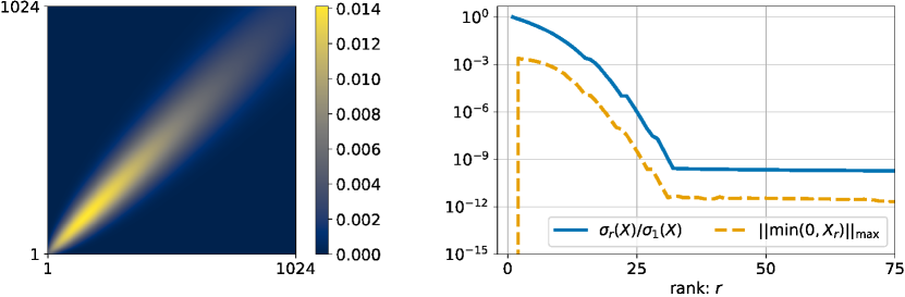
Figure 9: Properties of the discretised solution (9) to a two-component Smoluchowski equation: (left) the solution itself; (right) its normalised singular values and the modulus of the smallest negative entry of its best rank-$r$ approximation for varying $r$.

Alternating projections with different low-rank projections

Let us try to refine the best rank-$10$ approximation of $X$ to make it nonnegative. We compare 6 alternating-projection algorithms that use svd, rsvd with $p=2$, warm-started $\textsc{vol}_{w}$, cold-started $\textsc{vol}_{c}$, warm-started $\textsc{pvol}_{w}$ with $|I|=|J|=30$ and cold-started $\textsc{pvol}_{c}$ with $|I|=|J|=30$. For brevity, we will use the ap prefix to name the corresponding alternating-projection algorithms.

We care about two performance metrics. First, the rate at which the low-rank iterates $Y_{k}$ approach the nonnegative orthant. Second, the approximation error $\|X-Y_{k}\|_{\mathrm{F}}$ and how it compares with the initial error $\|X-Y_{0}\|_{\mathrm{F}}=\mathrm{dist}(X,\mathcal{M}_{10})$. We ran 10 random experiments with different random seeds for every type of the low-rank projection (except for svd) and performed 1000 iterations of the alternating projections. In Fig. 10, we show how the Frobenius norm of the negative elements $\|\min(0,Y_{k})\|_{\mathrm{F}}$ changes in the course of iterations by plotting its median together with the $25\%$ and $10\%$ percentiles. The median approximation errors after 10 and 1000 iterations are collected in Tab. 1.

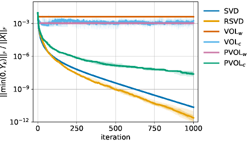
Figure 10: Convergence of the low-rank iterates $Y_{k}$ to $\mathbb{R}_{+}^{m\times n}$ for the alternating projections with inexact low-rank projections: the median, the $25\%$ and the $10\%$ percentiles.

Table 1: Median approximation errors of the low-rank iterates $Y_{k}$ after $10$ and $1000$ steps of alternating projections with inexact low-rank projections.

Error growth	svd	rsvd	$\textsc{vol}_{w}$	$\textsc{vol}_{c}$	$\textsc{pvol}_{w}$	$\textsc{pvol}_{c}$
$\tfrac{\|X-Y_{10}\|_{F}}{\|X-Y_{0}\|_{F}}$	$1.125$	$1.221$	$1.097$	$1.150$	$1.137$	$1.134$
$\tfrac{\|X-Y_{1000}\|_{F}}{\|X-Y_{0}\|_{F}}$	$1.132$	$1.226$	$1.097$	$4.834$	$1.139$	$1.144$

The linear convergence of ap-svd and ap-rsvd has already been observed in [70]. The warm-started $\textsc{ap-vol}_{w}$ and $\textsc{ap-pvol}_{w}$, however, fail to converge: it takes 1 iteration for the former and about 40 for the latter to reach the plateau. The explanation for such behaviour lies in the cross-approximation approach itself. While vol does not satisfy the interpolation property (8) per se when applied to a matrix of higher rank, it still interpolates the selected rows and columns. This means that $\textsc{ap-vol}_{w}$ at iteration $k>1$ deals with the rows $Y_{k}(I,:)$ and columns $Y_{k}(:,J)$ that are unaffected by the nonnegative projection and with the submatrix $Y_{k}(I,J)$ that has locally largest volume by construction. It follows that $Y_{k+1}=Y_{k}$, because vol does not know what happens outside of its index sets. The pvol algorithm with $|I|>r$ and $|J|>r$ loses the interpolation property whatsoever, but it is still likely that the index sets $I$ and $J$ will cease to change after a couple of iterations of $\textsc{ap-pvol}_{w}$ since the projective volume will be largely determined by the positive entries of the submatrix (provided that the negative entries are sufficiently small in the absolute value); with fixed $I$ and $J$, the alternating projections will only affect $Y_{k}(I,:)$ and $Y_{k}(:,J)$, making them nonnegative and staying ignorant to all the other entries of the matrix.

The main issue of $\textsc{ap-vol}_{w}$ and $\textsc{ap-pvol}_{w}$ is that only the local information drives the low-rank projection step. With cold-started alternating projections, we attempt to inject some global information into cross approximation. As Fig. 10 demonstrates, the freshly generated index sets are not sufficient to make $\textsc{ap-vol}_{c}$ converge to a nonnegative matrix: they only lead to irregular behaviour and growth of the approximation error (see Tab. 1). At the same time, $\textsc{ap-pvol}_{c}$ begins to converge, even if slower than ap-svd and ap-rsvd.

The approximation errors achieved with the convergent methods (ap-svd, ap-rsvd and $\textsc{ap-pvol}_{c}$) are only about $20\%$ larger than the error of the initial (best) approximation. Another observation from Tab. 1 is that most of the growth happens during the first 10 iterations.

Accelerated alternating projections

Thousand iterations were not enough for ap-svd and ap-rsvd to produce a nonnegative low-rank matrix. We can try to improve their convergence rates by modifying the alternating-projection framework itself. Since the nonnegative orthant $\mathbb{R}_{+}^{m\times n}$ is an obtuse convex cone, we can use the reflection-projection method [7]:

$$Z_{k+1}=2\cdot\Pi_{\mathbb{R}_{+}^{m\times n}}(Y_{k})-Y_{k},\quad Y_{k+1}\in\Pi_{\mathcal{M}_{r}}(Z_{k+1}),\quad k\geq 0.$$

Given that the nonnegative projection can be written entrywise as $\max(0,Y_{k})$, the reflection is nothing but the entrywise absolute value $|Y_{k}|$. The motivation behind this change is that the reflection pushes the current iterate towards the interior of $\mathbb{R}_{+}^{m\times n}$.

Another possibility is to replace the nonnegative projection with a scalar shift, which can be chosen based on how far $Y_{k}$ is from being nonnegative. We propose the shift-projection method with a parameter $\beta\geq 0$:

$$\alpha_{k}=\beta\cdot\|\min(0,Y_{k})\|_{\mathrm{max}},\quad Z_{k+1}=Y_{k}+\alpha_{k},\quad Y_{k+1}\in\Pi_{\mathcal{M}_{r}}(Z_{k+1}),\quad k\geq 0.$$

The additive shift is similar to the projection when it acts on the smallest negative entry and is similar to the reflection when it acts on the negative entries that are of the same order as the smallest one. However, unlike what happens with the projection and reflection, the positive entries change as well. In addition, the scalar shift increases the rank of $Y_{k}$ at most by one, so SVD-based projections can be applied to $Z_{k+1}$ efficiently.

Computing $\alpha_{k}$ is easy when we allow ourselves to explicitly form $Y_{k}$ by multiplying the low-rank factors—this is exactly what we try to avoid with vol and pvol, though. We can come up with a surrogate for $\|\min(0,Y_{k})\|_{\mathrm{max}}$ by applying rank-$1$ vol to $\mathrm{arccot}(Y_{k})$: the entry of largest absolute value in the transformed matrix corresponds to the smallest negative entry of the original matrix. To achieve better coverage, we start with a random initial position each time we calculate $\alpha_{k}$.

We test the modified schemes in the same settings as before. There are 18 algorithms to compare, which use 6 different low-rank projections and 3 versions of alternating projections: the original alternating projections, the reflection-projections and the shift-projections with $\beta=1/2$. We present the results in Fig. 11 and Tab. 2 with ap, rp and $\textsc{sp}(1/2)$.

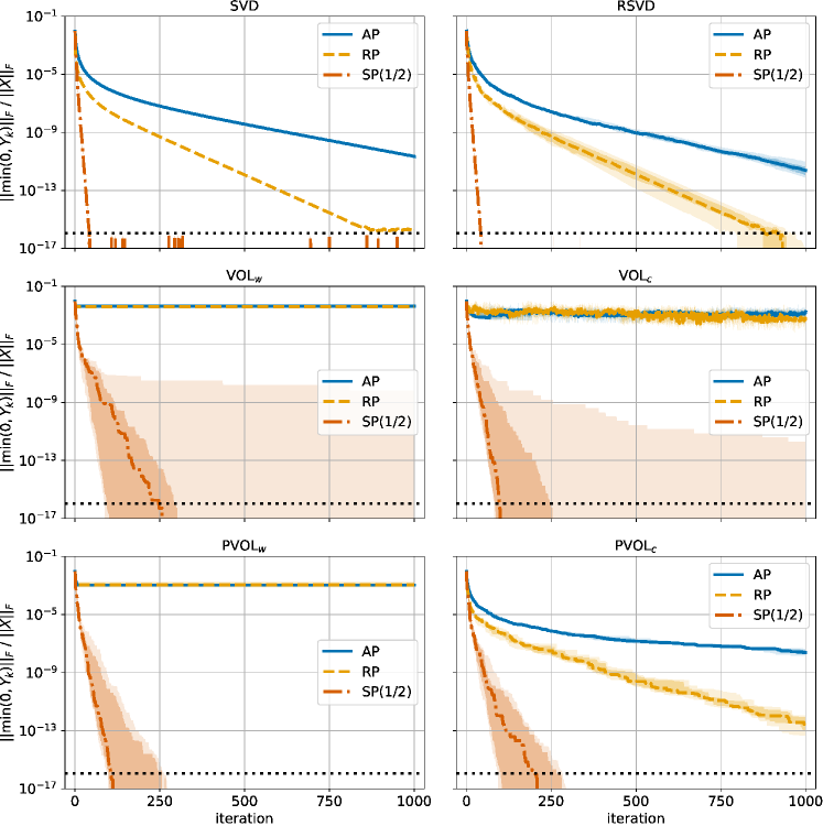
Figure 11: Convergence of the low-rank iterates $Y_{k}$ to the nonnegative orthant for the modified alternating-projection schemes with inexact low-rank projections: the median, the $25\%$ and the $10\%$ percentiles.

Table 2: Median approximation errors of the low-rank iterates $Y_{k}$ after $10/1000$ steps of modified alternating-projection schemes with inexact low-rank projections.

Modification	svd	rsvd	$\textsc{vol}_{w}$	$\textsc{vol}_{c}$	$\textsc{pvol}_{w}$	$\textsc{pvol}_{c}$
ap	$1.13/1.13$	$1.22/1.23$	$1.10/1.10$	$1.15/4.83$	$1.14/1.14$	$1.13/1.14$
rp	$1.19/1.19$	$1.48/1.48$	$1.33/1.33$	$2.35/9.41$	$1.24/1.24$	$1.23/1.23$
$\textsc{sp}(1/2)$	$5.78/5.78$	$5.78/5.78$	$5.55/5.76$	$5.62/5.79$	$5.60/5.79$	$5.65/5.79$

The first observation to make is that rp-svd, rp-rsvd and $\textsc{rp-pvol}_{c}$ converge faster than their original counterparts and produce slightly higher approximation errors. Next, $\textsc{sp}(1/2)$ converges after a finite number of steps for all 6 low-rank projections with the resulting approximation error about $5.5$ times larger than the initial error. The shift-projections appear to be ‘aggressive’ enough with injecting the global information to make the warm-started $\textsc{sp}(1/2)$-$\textsc{vol}_{w}$ and $\textsc{sp}(1/2)$-$\textsc{pvol}_{w}$ converge. The performance of the $\textsc{pvol}_{w}$ version is more consistent, though: unlike $\textsc{sp}(1/2)$-$\textsc{vol}_{w}$, it converged in each random experiment. We note again that the first few iterations are responsible for the growth of the approximation errors.

In Appendix D, we present results for one more alternating-projection scheme, which is known to converge in a finite number of steps for convex sets [88].

7.4.2 Tensor-train approximation

Next, we evaluate the performance of the accelerated versions of alternating projections by computing low-rank nonnegative TT approximations with ttsvd as the quasioptimal low-rank projection. Linear convergence of the classical alternating projections for this problem was numerically established in [101], where we also considered tensors in the Tucker format and randomised low-rank projections. A different approach was proposed in [59]: instead of computing quasioptimal projections onto the actual sets of interest that consist of tensors, the authors used the exact projections onto Cartesian products of sets that consist of matrices. Low-rank nonnegative TT approximations were also studied in [93].

We present an experiment that illustrates what happens to the negative elements during the iterations of alternating projections. Let $f\in\mathbb{R}_{+}^{1024}$ be a dicretised mixture of one-dimensional Gaussian probability densities in Fig. 12. We can consider $f$ as a tenth-order $2\times 2\times\ldots\times 2$ tensor and approximate it in the TT format—this gives the so-called quantised TT (QTT) approximation of the original vector. We compressed $f$ using ttsvd with relative accuracy $10^{-2}$ to get a QTT approximation of rank $\bm{r}=(2,2,2,3,3,4,5,4,2)$ and the actual relative approximation error of $6.97\cdot 10^{-3}$.

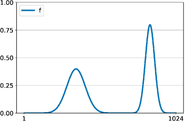
Figure 12: Mixture of one-dimensional Gaussian probability densities.

The QTT approximation produced by ttsvd contains negative entries, and Fig. 13 demonstrates that they appear as intervals rather than separate points. In Fig. 13, we compare the initial QTT approximation with the results of running 10 iterations of ap-ttsvd, rp-ttsvd and $\textsc{sp}(1/2)$-ttsvd. We see that even few iterations allow the methods to significantly reduce the number of negative elements in the tensor until only a handful of individual points is left. If we iterate further, the remaining entries decay at a linear rate, and the first 50 iterations are responsible for the most rapid decrease of their Frobenius norm (see Fig. 14). The approximation errors obtained with ap-ttsvd, rp-ttsvd and $\textsc{sp}(1/2)$-ttsvd increase

• $1.08$, $1.09$, $2.68$ times after 10 iterations and

• $1.09$, $1.09$, $2.68$ times after 1000 iterations, respectively.

Examples with another alternating-projection scheme, which converges in one iteration, can be found in Appendix D.

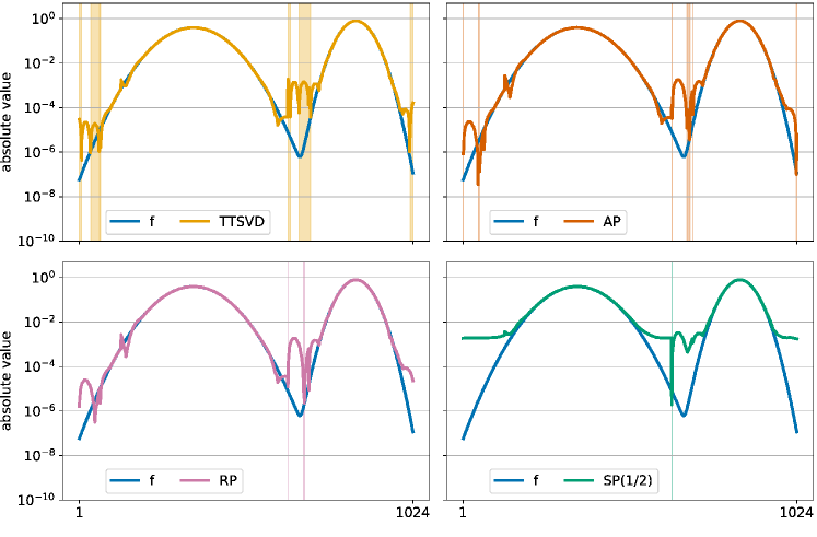
Figure 13: Mixture of one-dimensional Gaussian probability densities and the absolute value of its QTT approximations in log-scale with highlighted negative entries: the ttsvd approximation and its refinements after 10 iterations of ap-ttsvd, rp-ttsvd and $\textsc{sp}(1/2)$-ttsvd.

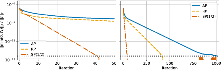
Figure 14: Convergence of the QTT approximations to the nonnegative orthant for the modified alternating-projection schemes based on ttsvd.

7.4.3 Regularised matrix completion

Out previous experiments demonstrate that the first iterations of alternating projections play a significant role in computing low-rank nonnegative approximations: most of the negative elements disappear during this stage, and the approximation error almost stabilises. This motivates us to incorporate a small number of iterations of alternating projections into various computational low-rank routines as a way to regularise their solutions towards nonnegativity.

Consider matrix completion as a model problem. Let $X_{*}\in\mathcal{M}_{r}$ be a low-rank matrix and $\Omega\subseteq\{1,\ldots,m\}\times\{1,\ldots,n\}$ be a set of index pairs. Assuming that we know only those entries of $X_{*}$ that reside in positions from $\Omega$, we aim to recover the whole matrix. One of the possible ways to approach the problem is via Riemannian optimisation [105].

Define $\Pi_{\Omega}(X)$ as the metric projection onto the set of sparse matrices supported on $\Omega$:

$$\Pi_{\Omega}(X)=\begin{cases}X(i,j),&(i,j)\in\Omega,\\ 0,&(i,j)\not\in\Omega.\end{cases}$$

Then we can attempt to recover $X_{*}$ by minimising the Frobenius norm on the sampling set:

$$\|\Pi_{\Omega}(X)-\Pi_{\Omega}(X_{*})\|_{\mathrm{F}}^{2}\to\min\quad\text{s.t.}\quad X\in\mathcal{M}_{r}.$$

This optimisation problem is posed on the smooth manifold $\mathcal{M}_{r}$, so we can use methods of Riemannian optimisation such as the Riemannian gradient descent:

$$X_{k+1}=\Pi_{\mathcal{M}_{r}}(X_{k}-\tau_{k}\Psi_{k}),\quad\Psi_{k}=\Pi_{T_{X_{k}}\mathcal{M}_{r}}\Big{(}\Pi_{\Omega}(X_{k})-\Pi_{\Omega}(X_{*})\Big{)}.$$

Compared with the usual gradient descent, the Riemannian version is different in two aspects: the Euclidean gradient $\Pi_{\Omega}(X_{k})-\Pi_{\Omega}(X_{*})$ is projected onto the tangent space $T_{X_{k}}\mathcal{M}_{r}$, and the resulting matrix after the gradient step is projected onto the manifold $\mathcal{M}_{r}$. We select the step size $\tau_{k}=\|\Psi_{k}\|_{\mathrm{F}}^{2}/\|\Pi_{\Omega}(\Psi_{k})\|_{\mathrm{F}}^{2}$ via the exact line search in the tangent space. The geometric nature of the algorithm makes it possible to make a gradient step without forming full matrices at the cost of $\mathcal{O}(\max(m,n)r^{2}+|\Omega|r)$ operations per iteration [105].

A crucial question is how many entries $|\Omega|$ we need to be able to recover $X_{*}$. The manifold $\mathcal{M}_{r}$ is of dimension $r(m+n-r)$, so at least this many samples are required, but in general we need $|\Omega|=\gamma\cdot r(m+n-r)$ with some $\gamma>1$. If we know some additional information about the matrix, we can try to use it to our advantage and reconstruct $X_{*}$ from a smaller sample.

Assume that $X_{*}$ is nonnegative. We propose to use a small number of warm-started $\textsc{ap-vol}_{w}$ iterations after each gradient step as regularisation. Crucially, the asymptotic complexity of the regularised Riemannian gradient descent remains the same. To test the idea, we fix $m=n=1000$, $r=5$ and generate 20 random nonnegative matrices $X_{*}$ as products of $n\times r$ low-rank factors with independent identically distributed entries from the uniform distribution on $(0,1/\sqrt{n})$. Next, for each value of the oversampling parameter $\gamma$ and each test matrix, we

• generate a set of index pairs $\Omega$ of size $\gamma\cdot r(m+n-r)$ uniformly at random with replacement,

• generate a rank-$r$ initial condition $X_{0}$ as a product of two $n\times r$ matrices with orthonormal columns that are selected uniformly at random with respect to the Haar measure,

• run 1000 iterations of the Riemannian gradient descent without regularisation,

• run 1000 iterations of the Riemannian gradient descent regularised with one iteration of $\textsc{ap-vol}_{w}$ after each gradient step.

For each value of $\gamma$, we calculate how many of the 20 problem instances converge to a matrix $X_{1000}$ such that $\|X_{1000}-X_{*}\|_{\mathrm{F}}<10^{-6}\cdot\|X_{*}\|_{\mathrm{F}}$ and plot the corresponding frequency of ‘success’. The results in Fig. 15 demonstrate that one iteration of $\textsc{ap-vol}_{w}$ makes it possible to recover low-rank nonnegative matrices from far fewer entries than the original Riemannian gradient descent without regularisation.

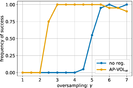
Figure 15: Riemannian matrix completion with alternating-projections regularisation can recover nonnegative matrices from fewer entries.

The impressive performance of $\textsc{ap-vol}_{w}$ for matrix completion suggests that fast alternating-projections algorithms can be used as regularisers for other problems in scientific computing. The most obvious possible extension is tensor completion in the TT format: the Riemannian optimisation approaches [98, 12] can be combined with alternating projections based on TT cross-approximation techniques [79, 27].

Regularisation based on alternating projections can also be applied to more general low-rank matrix and tensor recovery problems, where the goal is to reconstruct a low-rank object from some measurements. A particularly interesting example is non-parametric estimation of probability densities in low-rank tensor formats [90]. Among the used approaches that are used to ensure nonnegativity are some ad-hoc corrections [26] and the squared low-rank TT approximations [78, 20]—our idea can serve as an alternative.

Low-rank solvers for PDEs is another area where nonnegative regularisation can be used. The solutions to the chemical master equation [60], the Fokker–Planck equation [28] and the Smoluchowski equations [71] are naturally nonnegative, and the low-rank tensor solvers should preserve this property to keep the numerical solutions physically meaningful. In addition, the appearance of negative entries can lead to instabilities of the numerical time-stepping scheme and to potential blow-ups. It would be interesting to apply the method of alternating projections as a regulariser in these settings. In [69], the solution to a Smoluchowski coagulation equation is sought in the TT format with nonnegative cores. This, however, can lead to higher TT ranks and computational overhead.

7.5 Low-rank approximation in the maximum norm

How well can a matrix be approximated with a matrix of low rank? The usual answer is: look at the singular values. Their decay determines the smallest error of low-rank approximation in the spectral norm, the Frobenius norm and other unitarily invariant norms. Udell and Townsend addressed this question for the maximum norm (6), which is not unitarily invariant [104]. They proved that every $X\in\mathbb{R}^{n\times n}$ can be approximated with absolute error $\varepsilon\|X\|_{\mathrm{2}}$ in the maximum norm by a matrix of rank at most

$$r=\big{\lceil}72\log(1+2n)/\varepsilon^{2}\big{\rceil}.$$ (10)

When $\varepsilon$ is fixed, it is possible to compute a rank-one matrix $Y$ such that $\|X-Y\|_{\mathrm{\max}}\leq\varepsilon$, or decide that it does not exist, in a finite number of operations, but the problem is NP-hard in general [38]. Morozov et al. studied the problem of minimising the approximation error $\|X-Y\|_{\mathrm{\max}}$ over rank-one matrices [74]: they developed a method of alternating minimisation of the low-rank factors and analysed its convergence to the global minimum.

Less is understood when $r>1$. The individual steps of an alternating-minimisation method were studied in [108], but it is not proved that the iterations converge to the global minimum $\inf_{Y\in\mathcal{M}_{r}}\|X-Y\|_{\mathrm{\max}}$ for any non-trivial initial conditions. In a series of numerical experiments on random matrices with singular values in $(1,2)$, the authors of [108] studied a special case of approximation with $r=\sqrt{n}$ and observed that the numerically achieved error is bounded by

$$\inf_{Y\in\mathcal{M}_{r}}\|X-Y\|_{\mathrm{\max}}\leq\frac{\log^{0.6}(n)}{\sqrt{n}}.$$ (11)

This bound is asymptotically better than (10) by a factor of $n^{1/4}$.

We propose to numerically estimate $\min_{Y\in\mathcal{M}_{r}}\|X-Y\|_{\mathrm{\max}}$ with the method of alternating projections. For the given matrix $X\in\mathbb{R}^{m\times n}$ and rank $r<\mathrm{rank}(X)$, we choose an initial approximation $Y_{0}\in\mathcal{M}_{r}$ and set $\varepsilon_{+}=\|X-Y_{0}\|_{\mathrm{\max}}$ and $\varepsilon_{-}=0$. Now, we can perform a variant of binary search on the interval $(\varepsilon_{-},\varepsilon_{+}]$. We pick the middle of the interval $\varepsilon=\frac{1}{2}(\varepsilon_{-}+\varepsilon_{+})$ and run the method of (quasioptimal) alternating projections for the low-rank manifold $\mathcal{M}_{r}$ and the closed maximum-norm ball $B_{\varepsilon}(X)=\{Z\in\mathbb{R}^{m\times n}\leavevmode\nobreak\ :\leavevmode\nobreak\ \|X-Z\|_{\mathrm{\max}}\leq\varepsilon\}$. The projection onto $B_{\varepsilon}(X)$ can be computed as

$$\Pi_{B_{\varepsilon}(X)}(Y)=X+\Pi_{B_{\varepsilon}(0)}(Y-X)$$

and amounts to clipping the large entries of $Y-X$. We stop the iterations when the two consecutive errors become close

$$\|X-Y_{k}\|_{\mathrm{\max}}<(1+\delta)\cdot\|X-Y_{k-1}\|_{\mathrm{\max}},$$

increase $\varepsilon_{-}$ by a small amount such as $(\varepsilon_{+}-\varepsilon_{-})/50$ if the achieved approximation error $\|X-Y_{k}\|_{\mathrm{\max}}$ is not sufficiently close to $\varepsilon$, i.e.

$$\|X-Y_{k}\|_{\mathrm{\max}}>\varepsilon_{-}+\tfrac{2}{3}(\varepsilon_{+}-\varepsilon_{-})>\varepsilon_{-}+\tfrac{1}{2}(\varepsilon_{+}-\varepsilon_{-})=\varepsilon,$$

and update $\varepsilon_{+}$ with $\min\{\varepsilon_{+},\|X-Y_{k}\|_{\mathrm{\max}}\}$. We then repeat the process for the new interval $(\varepsilon_{-},\varepsilon_{+}]$ until it becomes small enough, at which point we conclude that

$$\inf_{Y\in\mathcal{M}_{r}}\|X-Y\|_{\mathrm{\max}}\leq\varepsilon_{+}.$$

This idea can be used as an alternative to the heuristic algorithm from [38] for the decision problem: we need to set the initial $\varepsilon_{+}$ to the desired value. We can also adapt the algorithm to other entrywise $\ell_{p}$ norms by projecting onto appropriate balls [97, 14, 64].

7.5.1 Orthogonal matrices

We test this alternating-projection method on two types of orthogonal matrices: the random orthogonal matrices and the identity matrix. First, we fix $n=1600$ and vary the rank. The initial conditions $Y_{0}$ are chosen as a product of two $n\times r$ random matrices with orthonormal columns in the random case and as a product of two $n\times r$ random Gaussian matrices with variance $1/r$ for the identity matrix. Note that we cannot initialise the iterations for the identity matrix with its best rank-$r$ approximation, because this leads to a loop. For the random orthogonal matrices, we perform 10 random experiments for every set of parameters and plot the median, the 25% and the 10% percentiles. For the identity matrices, we perform 5 random experiments and plot the minimum achieved error.

The results in Fig. 16 suggest that the approximation error decays as $1/\sqrt{r}$ for random orthogonal matrices and as $1/r$ for the identity matrices. In addition, we can compare our results with the numerical estimate (11): it gives $8.29\cdot 10^{-2}$ for $n=1600$ and $r=40$, while we have $5.72\cdot 10^{-2}$ for random orthogonal matrices and $3.11\cdot 10^{-1}$ for the identity matrices.

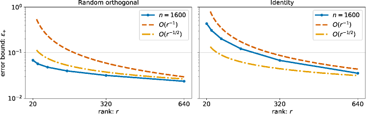
Figure 16: Errors of rank-$r$ approximation in the maximum norm achieved with ap-svd for $1600\times 1600$ matrices.

In the second series of experiments, we fix the rank $r=40$ and consider matrices of different sizes. In Fig. 17 we show the dependence of the maximum-norm approximation error achieved with ap-rsvd on the matrix size $n$. We observe that the error decays as $\log(n)/\sqrt{n}$ for random orthogonal matrices: larger matrices can be approximated with lower absolute maximum-norm error. Meanwhile, the approximation errors for the identity matrices grow as $\log^{2}(n)$.

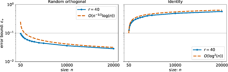
Figure 17: Errors of rank-$40$ approximation in the maximum norm achieved with ap-rsvd for $n\times n$ matrices.

The two classes of orthogonal matrices demonstrate qualitatively different behaviour in terms of the achievable approximation errors in the maximum norm. Both of them have spectral norms equal to one for every $n$; their maximum norms, however, are truly distinct. For the identity matrices, the maximum norm is also always equal to one. The maximum norm of a large $n\times n$ random orthogonal matrix $X$, upscaled by $\sqrt{n/\log(n)}$, converges in probability to 2 as $n\to\infty$ [58]. Consequently, the smallest low-rank approximation errors in the maximum norm converge to zero since $\inf_{Y\in\mathcal{M}_{r}}\|X-Y\|_{\mathrm{\max}}\leq\|X\|_{\mathrm{\max}}$ holds for every rank.

More numerical experiments are required to let us better understand how the above ultimate upper bound and the estimate (10) from [104] are related.

7.5.2 Quantised entries

The maximum norm is also useful in approximating matrices and tensors, whose entries are stored in the fixed-point format. These types of data appear in communication-intensive and resource-constrained applications such as wireless systems [57], distributed optimisation [76] and deep learning [35].

Every tensor with quantised entries can be seen as a rounded representation of a real-valued tensor, and our goal is to find one that is low-rank. Low-rank approximation of integer-valued matrices was considered in [38], where a block-coordinate descent method was used to approximate $n\times n$ matrices that are formed as products of standard Gaussian random low-rank factors of size $n\times r$ and then rounded entrywise to the nearest integer. When $n=200$ and the truncated SVD is chosen as the initial approximation, their method works in more than $90\%$ of random instances for $r\in\{1,20\}$, but never succeeds for $r\in\{2,5,10\}$.

We repeat the same experiments using the method of alternating projections, setting the initial value of $\varepsilon_{max}$ to $0.5$. The statistics, collected over 20 random instances of the problem, are collected in Tab. 3. Our approach succeeds every time for $r\in\{5,10,20\}$ and achieves lower approximation errors for $r=20$ than in [38].

Next, we consider the higher-order case of $100\times 100\times 100$ tensors that are formed as TT decompositions of rank $\bm{r}=(r,r)$ with standard Gaussian random TT cores and rounded entrywise to the nearest integer. We apply ap-ttsvd to 20 random tensors, initialised each time with a ttsvd-approximation of rank $\bm{r}$ (see Tab. 3). The alternating projections succeed for $r\in\{10,20\}$, but fail for $r=5$. Similar to [38], we observe that the higher the rank, the ‘easier’ the problem is to solve and the lower the achievable errors are.

It would also be interesting to test the method of alternating projections in situations where even less information is known: only signs [21] or phases [42].

Table 3: Approximation errors in the maximum norm for low-rank approximation of integer-valued matrices and tensors, achieved with alternating projections.

	Matrix			Tensor
Rank	Minimum	Mean	Maximum	Minimum	Mean	Maximum
5	$0.491$	$0.494$	$0.498$	$0.5007$	$0.5011$	$0.5017$
10	$0.468$	$0.473$	$0.482$	$0.4979$	$0.4988$	$0.4998$
20	$0.433$	$0.438$	$0.444$	$0.4851$	$0.4859$	$0.4876$

8 Conclusion and open problems

The main goal of our paper was to shed more light on why the simple and versatile method of alternating projections works so well in practice, where the numerically computed metric projections are never exact. With low-rank approximation of matrices and higher-order tensors in mind as the model problem, we developed a convergence theory that explains how the benign local geometry at the intersection of two sets can compensate for the wildly inexact nature of certain approximate projections. Our theory can, in turn, pave the way for the use of alternating projections in a wider range of applications. This point is neatly illustrated with the non-trivial numerical results that we obtained for regularised matrix completion and low-rank approximation in the maximum norm.

The theory is nowhere near complete though. An important question is whether the quasioptimal metric projection and the collection of points satisfying the normal-cone condition (7) of [66] impose equivalent constraints; this is true for hyperplanes, but how regular does the set need to be for this equivalence to hold? Among the directions of future research are to (i) study the convergence of quasioptimal alternating projections with less restrictive regularity constraints as in [8, 77] and (ii) incorporate quasioptimal metric projections into other optimisation methods such as the Douglas–Rachford algorithm [85, 51, 52, 4]. It still remains to apply the developed theory to analyse the convergence of quasioptimal alternating projections for low-rank nonnegative tensor approximation.

Alternating projections look very promising for constrained low-rank matrix and tensor approximation, especially when accelerated with shifts and cross-approximation. It would be of interest to employ this framework to regularise tensor-based numerical methods for PDEs and density estimation.

Appendix A Pythagorean property of prox-regular and convex sets

In this appendix we aim to improve the lower bound in Lemma 5.4 by considering sets that are more regular than super-regular. Namely, we will focus on prox-regularity and convexity.

A non-empty set $A\subseteq H$ is called prox-regular at $\hat{a}\in A$ if there exist $t>0$ and $\delta>0$ such that $A\cap{{\mathbb{B}}}_{\delta}(\hat{a})$ is closed in ${{\mathbb{B}}}_{\delta}(\hat{a})$ and

$$\langle v,a^{\prime}-a\rangle\leq\tfrac{t}{2}|a^{\prime}-a|^{2}\quad\text{for all}\quad a,a^{\prime}\in A\cap{{\mathbb{B}}}_{\delta}(\hat{a})\quad\text{and}\quad v\in N^{\mathrm{lim}}_{A}(a)\cap{{\mathbb{B}}}_{\delta}(0).$$

What we take as the definition of prox-regularity is proved in [87, Proposition 1.2] to be equivalent to the original definition proposed in [86]: that every point sufficiently close to $\hat{a}$ has a unique optimal metric projection. The class of prox-regular sets is large and includes smooth manifolds and convex sets. In addition, every prox-regular set is super-regular. This is easy to derive from another equivalent characterisation.

Lemma A.1.

Let $A\subseteq H$ be non-empty with $\hat{a}\in A$ and let $\delta>0$ be such that $A\cap{{\mathbb{B}}}_{\delta}(\hat{a})$ is closed in ${{\mathbb{B}}}_{\delta}(\hat{a})$. For $t>0$, the following properties are equivalent:

1. $\langle v,a^{\prime}-a\rangle\leq\frac{t}{2}|a^{\prime}-a|^{2}$ for all $a,a^{\prime}\in A\cap{{\mathbb{B}}}_{\delta}(\hat{a})$ and $v\in N^{\mathrm{lim}}_{A}(a)\cap{{\mathbb{B}}}_{\delta}(0)$;

2. $\langle v,a^{\prime}-a\rangle\leq\frac{t}{2\delta}|v|\cdot|a^{\prime}-a|^{2}$ for all $a,a^{\prime}\in A\cap{{\mathbb{B}}}_{\delta}(\hat{a})$ and $v\in N^{\mathrm{lim}}_{A}(a)$.

Proof.

The second property trivially implies the first one. By continuity, the first property holds for all $v\in N^{\mathrm{lim}}_{A}(a)$ with $|v|=\delta$ as well. Pick $v\in N^{\mathrm{lim}}_{A}(a)$. If $v=0$ then we are done; otherwise, scale it as $w=\tfrac{\delta}{|v|}v$ and plug into the first property to recover the second one. ∎

We also prove an analogue of Lemma 2.2 about the non-expansiveness of the projection [87, Proposition 3.1].

Lemma A.2.

Let $A\subseteq H$ be non-empty and prox-regular at $\hat{a}\in A$. Then there exist $t>0$ and $\delta>0$ such that for each $s\in(0,\min\{2,t\})$ and each $x\in{{\mathbb{B}}}_{s\delta/2t}(\hat{a})$ it holds that $\Pi_{A}(x)=\{\pi\}$ and

$$|\pi-a|\leq\tfrac{2}{2-s}|x-a|\quad\text{for every}\quad a\in A\cap{{\mathbb{B}}}_{s\delta/2t}(\hat{a}).$$

Proof.

First, we show that the optimal metric projection is unique. Let $\pi_{1},\pi_{2}\in\Pi_{A}(x)$, which exist by Lemma 2.1, assume they are distinct and consider

$$|\pi_{1}-x|^{2}=|\pi_{1}-\pi_{2}|^{2}+|\pi_{2}-x|^{2}-2\langle x-\pi_{2},\pi_{1}-\pi_{2}\rangle.$$

Choose $t$ and $\delta$ from the definition of prox-regularity. Since $|\pi_{1}-x|=|\pi_{2}-x|$, we get

$$|\pi_{1}-\pi_{2}|^{2}=2\langle x-\pi_{2},\pi_{1}-\pi_{2}\rangle\leq\tfrac{t}{\delta}|x-\pi_{2}|\cdot|\pi_{1}-\pi_{2}|^{2}<\tfrac{s}{2}|\pi_{1}-\pi_{2}|^{2}.$$

But $s\leq 2$, so we have a contradiction, and $\pi_{1}=\pi_{2}=\pi$.

Next, take $a\in A\cap{{\mathbb{B}}}_{s\delta/2t}(\hat{a})$ and expand the squared norm

$$|\pi-a|^{2}=\langle x-\pi,a-\pi\rangle+\langle\pi-a,x-a\rangle\leq\tfrac{t}{2\delta}|x-\pi|\cdot|\pi-a|^{2}+|x-a|\cdot|\pi-a|.$$

If $\pi=a$, we are done; else, divide and use $|x-\pi|\leq|x-a|$ to obtain

$$|x-a|\geq\left(1-\tfrac{t}{2\delta}|x-a|\right)|\pi-a|\geq\left(1-\tfrac{t}{2\delta}\tfrac{s\delta}{t}\right)|\pi-a|\geq\left(1-\tfrac{s}{2}\right)|\pi-a|.\qed$$

Lemma A.3.

Let $A\subseteq H$ be non-empty and prox-regular at $\hat{a}\in A$. Then there exist $t>0$ and $\delta>0$ such that for each $x\in{{\mathbb{B}}}_{s\delta/2t}(\hat{a})\setminus A$ with $s\in(0,\min\{2,t\})$ it holds that

$$\bigg{\langle}\frac{x-\pi}{|x-\pi|},\frac{x-a}{|x-a|}\bigg{\rangle}\geq\frac{|x-\pi|}{|x-a|}-\frac{2s}{(2-s)^{2}}$$

for $\Pi_{A}(x)=\{\pi\}$ and every $a\in A\cap{{\mathbb{B}}}_{s\delta/2t}(\hat{a})$.

Proof.

Repeat the proof of Lemma 5.4 and use Lemma A.2 instead of Lemma 2.2. ∎

Adding more regularity, we can obtain even tighter estimates. A non-empty set $A\subseteq H$ is called locally convex at $\hat{a}\in A$ if there exists a neighbourhood $\mathcal{V}$ of $\hat{a}$ such that $A\cap\mathcal{V}$ is convex. It is known [73, Proposition 1.5] that in this case

$$N^{\mathrm{lim}}_{A}(\hat{a})=\{v\in H\leavevmode\nobreak\ :\leavevmode\nobreak\ \langle v,a^{\prime}-\hat{a}\rangle\leq 0\quad\text{for all}\quad a^{\prime}\in A\cap\mathcal{V}\}.$$

Lemma A.4.

Let $A\subseteq H$ be non-empty, locally convex and locally closed at $\hat{a}\in A$. Then there exists $\delta>0$ such that for each $x\in{{\mathbb{B}}}_{\delta/2}(\hat{a})\setminus A$ it holds that

$$\bigg{\langle}\frac{x-\pi}{|x-\pi|},\frac{x-a}{|x-a|}\bigg{\rangle}\geq\frac{|x-\pi|}{|x-a|}$$

for $\Pi_{A}(x)=\{\pi\}$ and every $a\in A\cap{{\mathbb{B}}}_{\delta}(\hat{a})$.

Proof.

Pick $\delta>0$ such that $A\cap{{\mathbb{B}}}_{\delta}(\hat{a})$ is convex and closed in ${{\mathbb{B}}}_{\delta}(\hat{a})$. Then use the above characterisation of the limiting normal cone and note that $\Pi_{A}(x)=\Pi_{A\cap{{\mathbb{B}}}_{\delta}(\hat{a})}(x)$ for $x\in{{\mathbb{B}}}_{\delta/2}(\hat{a})$. Since $A\cap{{\mathbb{B}}}_{\delta}(\hat{a})$ is convex, there can be at most one optimal metric projection onto it. ∎

Appendix B Proof details

Proof of Lemma 2.1.

$\bm{1.}$ Let $x\in\mathcal{V}$ be a limit point of $A\cap\mathcal{V}$. Then $\mathrm{dist}(x,A)=0$ and there exists a sequence $(x_{n})\subset A\cap\mathcal{V}$ that converges to $x$. By assumption, there is a point $a\in A$ such that $\mathrm{dist}(x,a)=\mathrm{dist}(x,A)=0$. It follows that $x=a\in A$, but $x$ itself lies in $\mathcal{V}$ so $A\cap\mathcal{V}$ is closed in $\mathcal{V}$.

$\bm{2.}$ Pick an $x\in{{\mathbb{B}}}_{r/2}(\hat{a})$ and note that $\mathrm{dist}(x,A)\leq|x-\hat{a}|<r/2$. By definition of $\mathrm{dist}(x,A)$, there is a minimising sequence $(a_{n})\subset A$ such that $|x-a_{n}|\to\mathrm{dist}(x,A)$ as $n\to\infty$. Then

$$\limsup_{n\to\infty}|\hat{a}-a_{n}|\leq|x-\hat{a}|+\lim_{n\to\infty}|x-a_{n}|<\tfrac{r}{2}+\mathrm{dist}(x,A)<r.$$

By the Bolzano–Weierstrass theorem, there is a convergent subsequence $(a_{n_{k}})\subset{{\mathbb{B}}}_{r}(\hat{a})$. Since $A\cap{{\mathbb{B}}}_{r}(\hat{a})$ is closed in ${{\mathbb{B}}}_{r}(\hat{a})$, we have $\lim_{k\to\infty}a_{n_{k}}=a\in A\cap{{\mathbb{B}}}_{r}(\hat{a})$. By continuity of the norm,

$$|x-a|=\lim_{k\to\infty}|x-a_{n_{k}}|=\mathrm{dist}(x,A)$$

and $a\in\Pi_{A}(x)$. Finally, for every projection $\pi\in\Pi_{A}(x)$, we have

$$|\pi-\hat{a}|\leq|x-\pi|+|x-\hat{a}|\leq 2|x-\hat{a}|<r.\qed$$

Proof of Theorem 6.6: Implicit function theorem.

Consider a function

$$f(\varepsilon,\alpha,\beta)=2\varepsilon+\alpha\left(\tfrac{1}{\beta}-\varepsilon(1+\varepsilon)\right)+\sqrt{1-\alpha^{2}}\sqrt{1-\left(\tfrac{1}{\beta}-\varepsilon(1+\varepsilon)\right)^{2}}$$

and its partial derivatives

$$\frac{\partial f}{\partial\varepsilon}=2-\alpha(1+2\varepsilon)+\sqrt{1-\alpha^{2}}\frac{(1+2\varepsilon)\left(\tfrac{1}{\beta}-\varepsilon(1+\varepsilon)\right)}{\sqrt{1-\left(\tfrac{1}{\beta}-\varepsilon(1+\varepsilon)\right)^{2}}},$$

$$\frac{\partial f}{\partial\alpha}=\left(\tfrac{1}{\beta}-\varepsilon(1+\varepsilon)\right)-\frac{\alpha}{\sqrt{1-\alpha^{2}}}\sqrt{1-\left(\tfrac{1}{\beta}-\varepsilon(1+\varepsilon)\right)^{2}}.$$

Let $\hat{\alpha}\in(0,1)$, $\hat{\beta}>1$, and put $\varepsilon=0$. Then

$$\frac{\partial f}{\partial\varepsilon}(0,\hat{\alpha},\hat{\beta})=2-\hat{\alpha}+\frac{\sqrt{1-\hat{\alpha}^{2}}}{\sqrt{\hat{\beta}^{2}-1}}>0,\quad\frac{\partial f}{\partial\alpha}(0,\hat{\alpha},\hat{\beta})=\frac{1}{\hat{\beta}}\left(1-\frac{\hat{\alpha}}{\sqrt{1-\hat{\alpha}^{2}}}\sqrt{\hat{\beta}^{2}-1}\right).$$

We can apply the implicit function theorem to show that there is a $C^{\infty}$ function $\varepsilon(\alpha)$, defined in the neighbourhood of $\hat{\alpha}$, such that $f(\varepsilon(\alpha),\alpha,\hat{\beta})=f(0,\hat{\alpha},\hat{\beta})$ and

$$\varepsilon(\hat{\alpha})=0,\quad\frac{d\varepsilon}{d\alpha}(\hat{\alpha})=-\frac{\frac{\partial f}{\partial\alpha}(0,\hat{\alpha},\hat{\beta})}{\frac{\partial f}{\partial\varepsilon}(0,\hat{\alpha},\hat{\beta})}.$$

In addition, since $\alpha\mapsto\tfrac{\alpha}{\sqrt{1-\alpha^{2}}}$ is strictly increasing, the derivative $\tfrac{\partial f}{\partial\alpha}(0,\hat{\alpha},\hat{\beta})$ is positive if and only if $\hat{\alpha}\hat{\beta}<1$. Thus, $\varepsilon(\alpha)$ is strictly decreasing if and only if $\hat{\alpha}\hat{\beta}<1$. ∎

Appendix C Quasioptimal low-rank approximation: Details

C.1 Randomised SVD

The standard (and optimal in every unitarily invariant norm) way of computing a rank-$r$ approximation of a matrix is via the truncated SVD, which requires $\mathcal{O}(mn\cdot\min\{m,n\})$ operations. More efficient low-rank approximation algorithms of complexity $\mathcal{O}(\mathrm{nnz}(X)\cdot r)$ can be achieved with randomisation, where $\mathrm{nnz}(X)$ is the number of non-zero entries of $X$. One of the classics is the randomised range finder [48, Algorithm 4.1]: fix an oversampling parameter $p\geq 2$, generate an $n\times(r+p)$ random Gaussian matrix $\Omega$ and compute the QR decomposition of the product $QR=X\Omega$. It is then proved that [48, Theorem 10.5]

$$\mathbb{E}\|X-QQ^{*}X\|_{\mathrm{F}}\leq\sqrt{1+\frac{r}{p-1}}\cdot\mathrm{dist}(X,\mathcal{M}_{r}).$$

For $p=r+1$ the estimate turns into $\mathbb{E}\|X-QQ^{*}X\|_{\mathrm{F}}\leq\sqrt{2}\cdot\mathrm{dist}(X,\mathcal{M}_{r})$. Note, however, that the matrix $QQ^{*}X$ is of rank $r+p$ rather than $r$. To get a rank-$r$ approximation, we can compute the truncated SVD of $Q^{*}X$. The error of this randomised SVD was analysed in [46, Theorem 5.7] for a modification of the randomised range finder that uses $q$ steps of power iterations: that is the QR decomposition is computed for $(XX^{*})^{q}X\Omega$. We present an expected approximation error that is less tight than the one in [46], but more suitable for our needs:

$$\mathbb{E}\|X-Q\cdot\Pi_{\mathcal{M}_{r}}(Q^{*}X)\|_{\mathrm{F}}\leq\sqrt{1+144e^{2}(n-r)\frac{r(r+p)}{(p+1)^{2}}\left(\frac{\sigma_{r+1}}{\sigma_{r}}\right)^{4q}}\cdot\mathrm{dist}(X,\mathcal{M}_{r}).$$

Here, $\sigma_{r+1}\leq\sigma_{r}$ are the singular values of $X$. For $p=r-1$ the estimate simplifies to

$$\mathbb{E}\|X-Q\cdot\Pi_{\mathcal{M}_{r}}(Q^{*}X)\|_{\mathrm{F}}\leq\sqrt{1+288e^{2}(n-r)\left(\frac{\sigma_{r+1}}{\sigma_{r}}\right)^{4q}}\cdot\mathrm{dist}(X,\mathcal{M}_{r}).$$

Depending on the spectral gap and the number of power iterations, the randomised SVD can be expected to compute arbitrarily good quasioptimal projections onto $\mathcal{M}_{r}$. Note that the complexity of the algorithm grows linearly with $q$.

C.2 CUR and cross approximations

An alternative way to construct low-rank approximations is to use the columns and rows of the matrix itself. Recall the property of rank-$r$ matrices (8) that they can be represented with the help of $r$ rows and $r$ columns. The same idea can be used to compute a rank-$r$ approximation.

Choose $k_{c}\geq r$ columns $C=X(:,J)$, $k_{r}\geq r$ rows $R=X(I,:)$, and a generator matrix $U\in\mathbb{R}^{k_{c}\times k_{r}}$. The following is called a CUR approximation:

$$X\approx C\cdot U\cdot R$$

When the columns and rows are fixed, the optimal choice of the generator is [99]

$$\mathrm{argmin}_{U}\|X-CUR\|_{\mathrm{F}}=C^{\dagger}XR^{\dagger},$$

where $\dagger$ stands for the Moore–Penrose pseudoinverse. If $\mathrm{rank}(C^{\dagger}XR^{\dagger})=\mathrm{rank}(X)$, we recover the identity (8), since $C^{\dagger}XR^{\dagger}=X(I,J)^{-1}$ (see [49, Theorem A]); otherwise, the two generators are different. The CUR approximation with a non-optimal generator $X(I,J)^{\dagger}$ is known as the cross approximation:

$$X\approx C\cdot X(I,J)^{\dagger}\cdot R.$$

The approximation error achieved by the CUR and cross approximations depends on the choice of the index sets $I$ and $J$. It is shown in [25, Theorem 1.3] that every matrix $X$ with $\mathrm{rank}(X)\geq r$ contains $r$ columns $C=X(:,J)$ such that

$$\|X-CC^{\dagger}X\|_{\mathrm{F}}\leq\sqrt{1+r}\cdot\mathrm{dist}(X,\mathcal{M}_{r}).$$

Similarly, there are $r$ rows $R=X(I,:)$ that achieve

$$\|X-XR^{\dagger}R\|_{\mathrm{F}}\leq\sqrt{1+r}\cdot\mathrm{dist}(X,\mathcal{M}_{r}).$$

This proves the existence of a $\sqrt{2+2r}$-quasioptimal CUR approximation:

$$\|X-CC^{\dagger}XR^{\dagger}R\|_{\mathrm{F}}^{2}=\|X-CC^{\dagger}X\|_{\mathrm{F}}^{2}+\|CC^{\dagger}X-CC^{\dagger}XR^{\dagger}R\|_{\mathrm{F}}^{2}\leq 2(1+r)\cdot\mathrm{dist}(X,\mathcal{M}_{r})^{2}.$$

An analogous statement holds for the cross approximation [109]: there are index sets $I$ and $J$ of cardinality $r$ such that

$$\|X-C\cdot X(I,J)^{-1}\cdot R\|_{\mathrm{F}}\leq(1+r)\cdot\mathrm{dist}(X,\mathcal{M}_{r}).$$ (12)

In both cases, the corresponding rows and columns can be computed in polynomial time [19], though the complexities of $\mathcal{O}(mnr\cdot\min\{m,n\})$ and $\mathcal{O}(mnr\cdot\min\{m^{2},n^{2}\})$ operations, respectively, are higher than for the truncated SVD.

Better approximation can be achieved when we oversample the rows and columns. It is possible to construct a rank-$r$ CUR approximation based on $k_{c}=k_{r}=k>4r$ rows and columns that satisfies [10, Theorem 7.1]

$$\|X-CUR\|_{\mathrm{F}}\leq\sqrt{1+80\frac{r}{k-4r}}\cdot\mathrm{dist}(X,\mathcal{M}_{r}).$$

Therefore, we can reduce the approximation errors by taking larger $k$. The deterministic algorithm proposed in [10] has the complexity $\mathcal{O}(mnk\cdot\min\{m^{2},n^{2}\})$, which is similar to the cost of the cross approximation algorithm from [19]. It is also shown in [10, Theorem 8.1] that this quasioptimality estimate captures the correct relationship between the error and the oversampling: if $\|X-CUR\|_{\mathrm{F}}\leq\sqrt{1+\varepsilon}\cdot\mathrm{dist}(X,\mathcal{M}_{r})$ then $k_{r}$ and $k_{c}$ must scale as $r/\varepsilon$.

C.3 Maximum-volume principle

Back in Section 7.3 we motivated the need to work with quasioptimal low-rank matrix projections by saying that they can be faster than the truncated SVD. While the randomised SVD does indeed have a smaller computational complexity, the CUR- and cross-approximation algorithms that we have mentioned so far are slower than the optimal projection via the SVD.

The sampling strategy is the bottleneck. To decide which columns and rows to pick, each of them is assigned a specific score. And even though only the $\mathcal{O}(r)$ top scorers are chosen, the scores themselves are typically computed based on the left and right singular vectors. Hence, the SVD is required (at least if you want to prove strong quasioptimality estimates).

A different way of choosing the index sets $I$ and $J$ is based on maximising the volume of $X(I,J)$. The idea originates in the interpolation theory and leads to error estimates in the maximum norm [39, Corollary 2.3]: if the $r\times r$ matrix $X(I,J)$ satisfies

$$|\det X(I,J)|\geq\nu\cdot\max_{\hat{I},\hat{J}}|\det X(\hat{I},\hat{J})|$$

for some $\nu\leq 1$ then the error of cross approximation is bounded by

$$\|X-C\cdot X(I,J)^{-1}\cdot R\|_{\mathrm{\max}}\leq\frac{1+r}{\nu}\cdot\sigma_{r+1}(X).$$ (13)

Oversampling leads to better estimates [84, Theorem 7]. If the submatrix $X(I,J)\in\mathbb{R}^{k_{r}\times k_{c}}$ maximises the $r$-projective volume (the product of the $r$ largest singular values) among all the $k_{r}\times k_{c}$ submatrices of $X$ then

$$\|X-C\cdot\Pi_{\mathcal{M}_{r}}(X(I,J))^{\dagger}\cdot R\|_{\mathrm{\max}}\leq t(k_{r},r)t(k_{c},r)\cdot\sigma_{r+1}(X),$$

where

$$t(k,r)=\sqrt{1+\frac{r}{k-r+1}}.$$

Similar bounds hold in the spectral norm too [40, 84, 72].

In brief, cross approximation driven by the maximisation of volume is a powerful tool. Does it produce quasioptimal (in the Frobenius norm) low-rank projections, though? It is known that the bound (12) does not always hold for the submatrices of maximum volume [109]. Nevertheless, for a class of random matrices $X$ it was proved in [110] that the cross approximation based on the submatrix with the largest (generalised) $r$-projective volume delivers, in expectation, a $t(k_{r},r)t(k_{c},r)$-quasioptimal projection of $X$ onto $\mathcal{M}_{r}$.

Another quasioptimality result can be found in [50, Corollary 5.7]. When the row-indices $I$ and column-indices $J$ are selected to maximise the volume of the $k_{r}\times r$ submatrix of the $r$ dominant left singular vectors and of the $k_{c}\times r$ submatrix of the $r$ dominant right singular vectors, respectively, the error of the cross approximation can be estimated as

$$\|X-C\cdot\Pi_{\mathcal{M}_{r}}(X(I,J))^{\dagger}\cdot R\|_{\mathrm{F}}\leq\frac{3}{2}\Big{[}1+t(k_{r},r)+t(k_{c},r)+3t(k_{r},r)t(k_{c},r)\Big{]}\cdot\mathrm{dist}(X,\mathcal{M}_{r}),$$

provided that the spectral gap is large $\sigma_{r}(X)\geq 4t(k_{r},r)t(k_{c},r)\cdot\mathrm{dist}(X,\mathcal{M}_{r})$.

Thus, there is non-negligible support to treat cross approximation based on the maximum-volume principle as a quasioptimal low-rank projection. It remains to compute the corresponding index sets. Unfortunately, the problem is NP-hard [18]. On the bright side,

• the bound (13) from [39] suggests that a submatrix, whose volume is within a factor from the largest, suffices for a good approximation, and

• many of the results, including the estimates in [84] and the proof of quasioptimality for a class of random matrices from [110], hold for a submatrix of locally maximum volume, where ‘locally’ means that it is allowed to change one column and one row.

The maxvol algorithm of [41] and its generalisations to rectangular submatrices [82, 72] leverage both points and find $k_{r}$ rows in an $m\times r$ matrix such that the volume of the corresponding submatrix is within a prescribed factor $\nu$ from the locally maximum volume. The algorithm is iterative: the initialisation step takes $\mathcal{O}(m(k_{r}+r^{2}))$ operations, the cost of a single iteration is $\mathcal{O}(mk_{r})$ operations, and the number of iterations depends on $\nu$ and the initial guess of the rows.

This is the base of fast cross approximation. In the case of a square submatrix, $k_{r}=k_{c}=r$, we can update the row-indices $I$ and column-indices $J$ in an alternating fashion:

$$I\leftarrow\textsc{maxvol}(X(:,J),I),\quad J\leftarrow\textsc{maxvol}(X(I,:)^{T},J).$$ (14)

This procedure has the complexity of

$$\mathcal{O}\Big{(}(m+n)r^{2}\cdot N_{\mathrm{iterations}}+(m+n)r\cdot N_{\mathrm{interchanges}}\Big{)},$$

where $N_{\mathrm{iterations}}$ is the number of times the updates (14) are carried out and $N_{\mathrm{interchanges}}$ is the overall number of row-interchanges performed by maxvol.

The analogue for maximising the $r$-projective volume using $k_{r}\geq r$ rows and $k_{c}\geq r$ columns was proposed in [82]. There are two main differences. First, it is suggested to optimise $I$ and $J$ separately. To this end, two auxiliary index sets $I_{r}$ and $J_{r}$ of cardinality $r$ are needed. For the given $I$ and $J_{r}$, the first update is done as in (14):

$$I\leftarrow\textsc{maxvol}(X(:,J_{r}),I).$$

The second novelty is that the auxiliary indices $J_{r}$ are not updated with maxvol; instead, we use the dominant-r algorithm [82], which is a modification of the strong rank-revealing QR decomposition [47]:

$$J_{r}\leftarrow\textsc{dominant-r}(X(I,:),J_{r}).$$

The asymptotic complexity of dominant-r is identical to maxvol: $\mathcal{O}(n(k_{r}+r^{2}))$ operations for the initialisation, $\mathcal{O}(nk_{r})$ operations per iteration, and the number of interchanges, once again, depends on the quality of the initial guess of $J_{r}$ and on how close we want the volume to be to the locally maximum volume. Applying the same steps to $X^{T}$ in order to update $J$ and $I_{r}$, we get a submatrix of large $r$-projective volume; the complexity is

$$\mathcal{O}\Big{(}(m+n)(k_{r}+k_{c}+r^{2})\cdot N_{\mathrm{iterations}}+(m+n)(k_{r}+k_{c})\cdot N_{\mathrm{interchanges}}\Big{)}.$$

The bounds of the approximation errors tell us that $k_{r}$ and $k_{c}$ of order $r$ are sufficient.

Both cross-approximation algorithms scale linearly with $m$ and $n$. They do not require access to the whole $X$ by operating on submatrices of size $m\times r$ and $r\times n$. This means that we can keep $X$ out of memory and evaluate the submatrices on the fly. If $\mathrm{elem}(X)$ is the cost of computing a single element of $X$, the complexities—with $k_{r}=\mathcal{O}(r)$ and $k_{c}=\mathcal{O}(r)$—become

$$\mathcal{O}\Big{(}(m+n)(r^{2}+r\cdot\mathrm{elem}(X))\cdot N_{\mathrm{iterations}}+(m+n)r\cdot N_{\mathrm{interchanges}}\Big{)}.$$

The fact that only a small portion of adaptively chosen entries of a matrix make it possible to construct a good low-rank approximation is impressive, but it would be even more so for tensors, since it becomes prohibitive to store all $\prod_{k=1}^{d}n_{k}$ elements for large $d$. In [79], the maximum-volume principle is extended to the tensor-train (TT) format. This leads to a fast cross-approximation algorithm that is based on the successive application of maxvol to the unfoldings of the tensor. The complexity of the proposed method is

$$\mathcal{O}\Big{(}dn(r^{3}+r^{2}\cdot\mathrm{elem}(\bm{X}))\cdot N_{\mathrm{iterations}}+dnr^{2}\cdot N_{\mathrm{interchanges}}\Big{)},$$

which scales linearly with the number of dimensions $d$—merely $\mathcal{O}(dnr^{2})$ entries of the tensor are sampled. In addition, the dependence on the rank has increased by one order compared to the matrix case. The explanation is in the TT decomposition itself: $d-2$ of its TT cores are tensors of size $r\times n\times r$, while the remaining two are matrices. The approximation errors of the TT-cross approximation in the maximum norm were studied in [91, 83].

Appendix D Low-rank nonnegative approximation: More tests

One more option to modify the method of alternating projections

$$Z_{k+1}=\Pi_{\mathbb{R}_{+}^{m\times n}}(Y_{k}),\quad Y_{k+1}\in\Pi_{\mathcal{M}_{r}}(Z_{k+1}),\quad k\geq 0,$$

is to compute the projection onto the translate of $\mathbb{R}_{+}^{m\times n}$ so that $Z_{k+1}$ ends up in the interior. We write the method of indentation-projection as

$$\alpha_{k}=\beta\cdot\|\min(0,Y_{k})\|_{\mathrm{max}},\quad Z_{k+1}=\Pi_{\alpha_{k}+\mathbb{R}_{+}^{m\times n}}(Y_{k}),\quad Y_{k+1}\in\Pi_{\mathcal{M}_{r}}(Z_{k+1}),\quad k\geq 0.$$

Basically, $Z_{k+1}=\max(\alpha_{k},Y_{k})$ so that the negative entries of $Y_{k}$ are pushed farther than by the shift-projection method, but the positive entries stay intact. Such iterations are known to converge in a finite number of steps for two convex sets [88].

We repeat the experiments of Section 7.4 about the two-component Smoluchowski equation using indentation-projections with $\beta=3/4$. The results in Fig. 18 and Tab. 4, which are extended versions of Fig. 11 and Tab. 2 from the main text, show that indentation-projections improve the convergence rates for svd, rsvd, and $\textsc{pvol}_{c}$ while increasing the approximation error three times. The warm-started $\textsc{ip}(3/4)$-$\textsc{vol}_{w}$ and $\textsc{ip}(3/4)$-$\textsc{pvol}_{w}$ keep stagnating, and the cold-started $\textsc{ip}(3/4)$-$\textsc{vol}_{c}$ exhibits irregular behaviour.

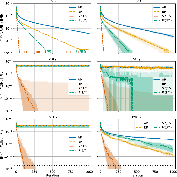
Figure 18: Convergence of the low-rank iterates $Y_{k}$ to the nonnegative orthant for the modified alternating-projection schemes with inexact low-rank projections: the median, the $25\%$ and the $10\%$ percentiles.

Table 4: Median approximation errors of the low-rank iterates $Y_{k}$ after $10/1000$ steps of modified alternating-projection schemes with inexact low-rank projections.

Modification	svd	rsvd	$\textsc{vol}_{w}$	$\textsc{vol}_{c}$	$\textsc{pvol}_{w}$	$\textsc{pvol}_{c}$
ap	$1.13/1.13$	$1.22/1.23$	$1.10/1.10$	$1.15/4.83$	$1.14/1.14$	$1.13/1.14$
rp	$1.19/1.19$	$1.48/1.48$	$1.33/1.33$	$2.35/9.41$	$1.24/1.24$	$1.23/1.23$
$\textsc{sp}(1/2)$	$5.78/5.78$	$5.78/5.78$	$5.55/5.76$	$5.62/5.79$	$5.60/5.79$	$5.65/5.79$
$\textsc{ip}(3/4)$	$3.11/3.11$	$3.21/3.21$	$4.41/4.86$	$6.85/7.08$	$3.11/3.11$	$3.04/3.04$

We also apply indentation-projections to compute a nonnegative QTT approximation of the mixture of Gaussian probability densities from Section 7.4: the method converges in one iteration and the approximation error grows $1.44$ times (see Fig. 19).

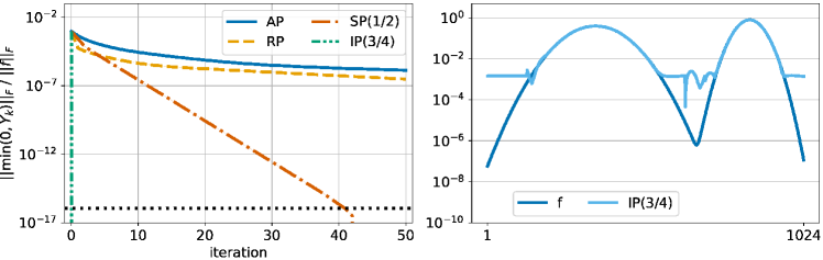
Figure 19: The nonnegative QTT approximation obtained with the method of indentation-projections based on ttsvd.

References

- [1] S. Adly, F. Nacry and L. Thibault “Preservation of prox-regularity of sets with applications to constrained optimization” In SIAM J. Optim. 26.1 SIAM, 2016, pp. 448–473
- [2] S. Agmon “The relaxation method for linear inequalities” In Can. J. Math. 6 Cambridge University Press, 1954, pp. 382–392
- [3] F. Andersson and M. Carlsson “Alternating projections on nontangential manifolds” In Constr. Approx. 38.3 Springer, 2013, pp. 489–525
- [4] F.J. Aragón Artacho, R. Campoy and M.K. Tam “The Douglas–Rachford algorithm for convex and nonconvex feasibility problems” In Math. Methods Oper. Res. 91 Springer, 2020, pp. 201–240
- [5] H.H. Bauschke and P.L. Combettes “Convex Analysis and Monotone Operator Theory in Hilbert Spaces” New York: Springer, 2011
- [6] H.H. Bauschke, P.L. Combettes and D.R. Luke “Phase retrieval, error reduction algorithm, and Fienup variants: a view from convex optimization” In J. Opt. Soc. Am. A 19.7 Optica Publishing Group, 2002, pp. 1334–1345
- [7] H.H. Bauschke and S.G. Kruk “Reflection-projection method for convex feasibility problems with an obtuse cone” In J. Optim. Theory Appl. 120.3 Springer, 2004, pp. 503–531
- [8] H.H. Bauschke, D.R. Luke, H.M. Phan and X. Wang “Restricted normal cones and the method of alternating projections: theory” In Set-Valued Var. Anal. 21.3 Springer, 2013, pp. 431–473
- [9] L.B. Beasley and T.J. Laffey “Real rank versus nonnegative rank” In Linear Algebra Appl. 431.12 Elsevier, 2009, pp. 2330–2335
- [10] C. Boutsidis and D.P. Woodruff “Optimal CUR matrix decompositions” In Proceedings of the 46th annual ACM symposium on Theory of computing, 2014, pp. 353–362
- [11] L.M. Bregman “The method of successive projections for finding a common point of convex sets” In Soviet Math. Dokl. 6, 1965, pp. 688–692
- [12] Stanislav Budzinskiy and Nikolai Zamarashkin “Tensor train completion: Local recovery guarantees via Riemannian optimization” In Numer. Linear Algebra Appl., 2023, pp. e2520
- [13] W. Cheney and A.A. Goldstein “Proximity maps for convex sets” In Proc. Am. Math. Soc. 10.3, 1959, pp. 448–450
- [14] F. Chierichetti et al. “Algorithms for low-rank approximation” In International Conference on Machine Learning, 2017, pp. 806–814
- [15] M. Chu, N. Del Buono, L. Lopez and T. Politi “On the low-rank approximation of data on the unit sphere” In SIAM J. Matrix Anal. Appl. 27.1 SIAM, 2005, pp. 46–60
- [16] M.T. Chu, R.E. Funderlic and R.J. Plemmons “Structured low rank approximation” In Linear Algebra Appl. 366 Elsevier, 2003, pp. 157–172
- [17] A. Cichocki, R. Zdunek, A.H. Phan and S. Amari “Nonnegative matrix and tensor factorizations: Applications to exploratory multi-way data analysis and blind source separation” Chichester: John Wiley & Sons, 2009
- [18] A. Civril and M. Magdon-Ismail “On selecting a maximum volume sub-matrix of a matrix and related problems” In Theor. Comput. Sci. 410.47-49 Elsevier, 2009, pp. 4801–4811
- [19] A. Cortinovis and D. Kressner “Low-rank approximation in the Frobenius norm by column and row subset selection” In SIAM J. Matrix Anal. Appl. 41.4 SIAM, 2020, pp. 1651–1673
- [20] T. Cui and S. Dolgov “Deep composition of Tensor-Trains using squared inverse Rosenblatt transports” In Found. Comput. Math. 22.6 Springer, 2022, pp. 1863–1922
- [21] M.A. Davenport, Y. Plan, E. Van Den Berg and M. Wootters “1-bit matrix completion” In Inf. Inference: J. IMA 3.3 OUP, 2014, pp. 189–223
- [22] L. De Lathauwer, B. De Moor and J. Vandewalle “A multilinear singular value decomposition” In SIAM J. Matrix Anal. Appl. 21.4 SIAM, 2000, pp. 1253–1278
- [23] L. De Lathauwer, B. De Moor and J. Vandewalle “On the best rank-1 and rank-(, , …, ) approximation of higher-order tensors” In SIAM J. Matrix Anal. Appl. 21.4 SIAM, 2000, pp. 1324–1342
- [24] J.W. Demmel “Applied Numerical Linear Algebra” Philadelphia: SIAM, 1997
- [25] A. Deshpande, L. Rademacher, S.S. Vempala and G. Wang “Matrix approximation and projective clustering via volume sampling” In Theory Comput. 2.1 Theory of Computing Exchange, 2006, pp. 225–247
- [26] S. Dolgov, K. Anaya-Izquierdo, C. Fox and R. Scheichl “Approximation and sampling of multivariate probability distributions in the tensor train decomposition” In Stat. Comput. 30 Springer, 2020, pp. 603–625
- [27] S. Dolgov and D. Savostyanov “Parallel cross interpolation for high-precision calculation of high-dimensional integrals” In Comput. Phys. Commun. 246 Elsevier, 2020, pp. 106869
- [28] S.V. Dolgov, B.N. Khoromskij and I.V. Oseledets “Fast solution of parabolic problems in the tensor train/quantized tensor train format with initial application to the Fokker–Planck equation” In SIAM J. Sci. Comput. 34.6 SIAM, 2012, pp. A3016–A3038
- [29] J. Dongarra et al. “The singular value decomposition: Anatomy of optimizing an algorithm for extreme scale” In SIAM Rev. 60.4 SIAM, 2018, pp. 808–865
- [30] D. Drusvyatskiy, A.D. Ioffe and A.S. Lewis “Alternating projections and coupling slope”, 2014 arXiv:1401.7569
- [31] D. Drusvyatskiy, A.D. Ioffe and A.S. Lewis “Transversality and alternating projections for nonconvex sets” In Found. Comput. Math. 15.6 Springer, 2015, pp. 1637–1651
- [32] D. Drusvyatskiy and A.S. Lewis “Local linear convergence for inexact alternating projections on nonconvex sets” In Vietnam J. Math. 47 Springer, 2019, pp. 669–681
- [33] R. Escalante and M. Raydan “Alternating projection methods” Philadelphia: SIAM, 2011
- [34] X. Fu, K. Huang, N.D. Sidiropoulos and W.-K. Ma “Nonnegative matrix factorization for signal and data analytics: Identifiability, algorithms, and applications.” In IEEE Signal Process. Mag. 36.2, 2019, pp. 59–80
- [35] A. Gholami et al. “A survey of quantization methods for efficient neural network inference” In Low-Power Computer Vision, 2022, pp. 291–326
- [36] N. Gillis “Nonnegative matrix factorization” Philadelphia: SIAM, 2020
- [37] N. Gillis and R. Rajkó “Partial identifiability for nonnegative matrix factorization” In SIAM J. Matrix Anal. Appl. 44.1 SIAM, 2023, pp. 27–52
- [38] N. Gillis and Y. Shitov “Low-rank matrix approximation in the infinity norm” In Linear Algebra Appl. 581 Elsevier, 2019, pp. 367–382
- [39] S.A. Goreinov and E.E. Tyrtyshnikov “The maximal-volume concept in approximation by low-rank matrices” In Structured Matrices in Mathematics, Computer Science, and Engineering, I Providence: AMS, 2001, pp. 47–51
- [40] S.A. Goreinov, E.E. Tyrtyshnikov and N.L. Zamarashkin “A theory of pseudoskeleton approximations” In Linear Algebra Appl. 261.1-3 Elsevier, 1997, pp. 1–21
- [41] S.A. Goreinov et al. “How to find a good submatrix” In Matrix Methods: Theory, Algorithms And Applications: Dedicated to the Memory of Gene Golub Singapore: World Scientific, 2010, pp. 247–256
- [42] A.P. Goucha and J. Gouveia “The phase rank of a matrix”, 2021 arXiv:2111.01962
- [43] I. Grubišić and R. Pietersz “Efficient rank reduction of correlation matrices” In Linear Algebra Appl. 422.2-3 Elsevier, 2007, pp. 629–653
- [44] C. Grussler and A. Rantzer “On optimal low-rank approximation of non-negative matrices” In 2015 54th IEEE Conference on Decision and Control (CDC), 2015, pp. 5278–5283
- [45] C. Grussler, A. Rantzer and P. Giselsson “Low-rank optimization with convex constraints” In IEEE Trans. Autom. Control 63.11 IEEE, 2018, pp. 4000–4007
- [46] M. Gu “Subspace iteration randomization and singular value problems” In SIAM J. Sci. Comput. 37.3 SIAM, 2015, pp. A1139–A1173
- [47] M. Gu and S.C. Eisenstat “Efficient algorithms for computing a strong rank-revealing QR factorization” In SIAM J. Sci. Comput. 17.4 SIAM, 1996, pp. 848–869
- [48] N. Halko, P.-G. Martinsson and J.A. Tropp “Finding structure with randomness: Probabilistic algorithms for constructing approximate matrix decompositions” In SIAM Rev. 53.2 SIAM, 2011, pp. 217–288
- [49] K. Hamm and L. Huang “Perspectives on CUR decompositions” In Appl. Comput. Harmon. Anal. 48.3 Elsevier, 2020, pp. 1088–1099
- [50] K. Hamm and L. Huang “Perturbations of CUR decompositions” In SIAM J. Matrix Anal. Appl. 42.1 SIAM, 2021, pp. 351–375
- [51] R. Hesse and D.R. Luke “Nonconvex notions of regularity and convergence of fundamental algorithms for feasibility problems” In SIAM J. Optim. 23.4 SIAM, 2013, pp. 2397–2419
- [52] R. Hesse, D.R. Luke and P. Neumann “Alternating projections and Douglas-Rachford for sparse affine feasibility” In IEEE Trans. Signal Process. 62.18 IEEE, 2014, pp. 4868–4881
- [53] N.J. Higham “Accuracy and Stability of Numerical Algorithms” Philadelphia: SIAM, 2002
- [54] N.J. Higham “Computing the nearest correlation matrix—a problem from finance” In IMA J. Numer. Anal. 22.3 OUP, 2002, pp. 329–343
- [55] S. Holtz, T. Rohwedder and R. Schneider “On manifolds of tensors of fixed TT-rank” In Numer. Math. 120.4 Springer, 2012, pp. 701–731
- [56] P. Hrubeš “On the nonnegative rank of distance matrices” In Inf. Process. Lett. 112.11 Elsevier, 2012, pp. 457–461
- [57] S. Jacobsson et al. “Quantized precoding for massive MU-MIMO” In IEEE Trans. Commun. 65.11 IEEE, 2017, pp. 4670–4684
- [58] T. Jiang “Maxima of entries of Haar distributed matrices” In Probab. Theory Relat. Fields 131 Springer, 2005, pp. 121–144
- [59] T.-X. Jiang, M.K. Ng, J. Pan and G.-J. Song “Nonnegative low rank tensor approximations with multidimensional image applications” In Numer. Math. 153.1 Springer, 2023, pp. 141–170
- [60] V. Kazeev, M. Khammash, M. Nip and C. Schwab “Direct solution of the chemical master equation using quantized tensor trains” In PLoS Comput. Biol. 10.3 Public Library of Science San Francisco, USA, 2014, pp. e1003359
- [61] Tamara G Kolda and Brett W Bader “Tensor decompositions and applications” In SIAM Rev. 51.3 SIAM, 2009, pp. 455–500
- [62] A.Y. Kruger, D.R. Luke and N.H. Thao “Set regularities and feasibility problems” In Math. Program. 168 Springer, 2018, pp. 279–311
- [63] A.Y. Kruger and N.H. Thao “Regularity of collections of sets and convergence of inexact alternating projections”, 2015 arXiv:1501.04191
- [64] A. Kyrillidis “Simple and practical algorithms for -norm low-rank approximation”, 2018 arXiv:2108.12163
- [65] J.M. Lee “Introduction to Smooth Manifolds”, Graduate Texts in Mathematics New York: Springer, 2003
- [66] A. Lewis, D.R. Luke and J. Malick “Local linear convergence of alternating and averaged nonconvex projections” In Found. Comput. Math. 9.4, 2009, pp. 485–513
- [67] A.S. Lewis and J. Malick “Alternating projections on manifolds” In Math. Oper. Res. 33.1 INFORMS, 2008, pp. 216–234
- [68] D.R. Luke “Prox-regularity of rank constraint sets and implications for algorithms” In J. Math. Imaging Vis. 47 Springer, 2013, pp. 231–238
- [69] G. Manzini, E. Skau, D.P. Truong and R. Vangara “Nonnegative tensor-train low-rank approximations of the Smoluchowski coagulation equation” In International Conference on Large-Scale Scientific Computing, 2021, pp. 342–350
- [70] S. Matveev and S. Budzinskiy “Sketching for a low-rank nonnegative matrix approximation: Numerical study” In Russ. J. Numer. Anal. Math. Model. 38.2 De Gruyter, 2023, pp. 99–114
- [71] S.A. Matveev, D.A. Zheltkov, E.E. Tyrtyshnikov and A.P. Smirnov “Tensor train versus Monte Carlo for the multicomponent Smoluchowski coagulation equation” In J. Comput. Phys. 316 Elsevier, 2016, pp. 164–179
- [72] A. Mikhalev and I.V. Oseledets “Rectangular maximum-volume submatrices and their applications” In Linear Algebra Appl. 538 Elsevier, 2018, pp. 187–211
- [73] B.S. Mordukhovich “Variational Analysis and Generalized Differentiation I: Basic Theory” Berlin: Springer, 2006
- [74] Stanislav Morozov, Matvey Smirnov and Nikolai Zamarashkin “On the optimal rank-1 approximation of matrices in the Chebyshev norm” In Linear Algebra Appl. 679 Elsevier, 2023, pp. 4–29
- [75] T.. Motzkin and I.J. Schoenberg “The relaxation method for linear inequalities” In Can. J. Math. 6 Cambridge University Press, 1954, pp. 393–404
- [76] A. Nedic, A. Olshevsky, A. Ozdaglar and J.N. Tsitsiklis “On distributed averaging algorithms and quantization effects” In IEEE Trans. Autom. Control 54.11 IEEE, 2009, pp. 2506–2517
- [77] Dominikus Noll and Aude Rondepierre “On local convergence of the method of alternating projections” In Found. Comput. Math. 16 Springer, 2016, pp. 425–455
- [78] G.S. Novikov, M.E. Panov and I.V. Oseledets “Tensor-train density estimation” In Uncertainty in artificial intelligence, 2021, pp. 1321–1331
- [79] I. Oseledets and E. Tyrtyshnikov “TT-cross approximation for multidimensional arrays” In Linear Algebra Appl. 432.1 Elsevier, 2010, pp. 70–88
- [80] I.V. Oseledets “Tensor-train decomposition” In SIAM J. Sci. Comput. 33.5 SIAM, 2011, pp. 2295–2317
- [81] I.V. Oseledets and E.E. Tyrtyshnikov “Breaking the curse of dimensionality, or how to use SVD in many dimensions” In SIAM J. Sci. Comput. 31.5 SIAM, 2009, pp. 3744–3759
- [82] A. Osinsky “Rectangular maximum volume and projective volume search algorithms”, 2018 arXiv:1809.02334
- [83] A.I. Osinsky “Tensor trains approximation estimates in the Chebyshev norm” In Comput. Math. Math. Phys. 59.2 Springer, 2019, pp. 201–206
- [84] A.I. Osinsky and N.L. Zamarashkin “Pseudo-skeleton approximations with better accuracy estimates” In Linear Algebra Appl. 537 Elsevier, 2018, pp. 221–249
- [85] H.M. Phan “Linear convergence of the Douglas–Rachford method for two closed sets” In Optimization 65.2 Taylor & Francis, 2016, pp. 369–385
- [86] R. Poliquin and R. Rockafellar “Prox-regular functions in variational analysis” In Trans. Am. Math. Soc. 348.5, 1996, pp. 1805–1838
- [87] R. Poliquin, R. Rockafellar and L. Thibault “Local differentiability of distance functions” In Trans. Am. Math. Soc. 352.11, 2000, pp. 5231–5249
- [88] M.A. Rami, U. Helmke and J.B. Moore “A finite steps algorithm for solving convex feasibility problems” In J. Glob. Optim. 38 Springer, 2007, pp. 143–160
- [89] R.T. Rockafellar and R.J.-B. Wets “Variational Analysis” Berlin: Springer, 2009
- [90] P.B. Rohrbach, S. Dolgov, L. Grasedyck and R. Scheichl “Rank bounds for approximating Gaussian densities in the tensor-train format” In SIAM/ASA J. Uncertain. Quantif. 10.3 SIAM, 2022, pp. 1191–1224
- [91] D.V. Savostyanov “Quasioptimality of maximum-volume cross interpolation of tensors” In Linear Algebra Appl. 458 Elsevier, 2014, pp. 217–244
- [92] Ulrich Schollwöck “The density-matrix renormalization group in the age of matrix product states” In Ann. Phys. 326.1 Elsevier, 2011, pp. 96–192
- [93] E.M. Shcherbakova and E.E. Tyrtyshnikov “Fast Nonnegative Tensor Factorizations with Tensor Train Model” In Lobachevskii J. Math. 43.4 Springer, 2022, pp. 882–894
- [94] Y. Shitov “Euclidean distance matrices and separations in communication complexity theory” In Discrete Comput. Geom. 61 Springer, 2019, pp. 653–660
- [95] G. Song, M.K. Ng and T.-X. Jiang “Tangent space based alternating projections for nonnegative low rank matrix approximation” In IEEE Trans. Knowl. Data Eng. IEEE, 2022, pp. 1–18
- [96] G.-J. Song and M.K. Ng “Nonnegative low rank matrix approximation for nonnegative matrices” In Appl. Math. Lett. 105 Elsevier, 2020, pp. 106300
- [97] Z. Song, D.P. Woodruff and P. Zhong “Low rank approximation with entrywise -norm error” In Proceedings of the 49th Annual ACM SIGACT Symposium on Theory of Computing, 2017, pp. 688–701
- [98] M. Steinlechner “Riemannian optimization for high-dimensional tensor completion” In SIAM J. Sci. Comput. 38.5 SIAM, 2016, pp. S461–S484
- [99] G.W. Stewart “Four algorithms for the the efficient computation of truncated pivoted QR approximations to a sparse matrix” In Numer. Math. 83 Springer, 1999, pp. 313–323
- [100] T. Strohmer and R. Vershynin “A randomized Kaczmarz algorithm with exponential convergence” In J. Fourier Anal. Appl. 15.2 Springer, 2009, pp. 262
- [101] A. Sultonov, S. Matveev and S. Budzinskiy “Low-rank nonnegative tensor approximation via alternating projections and sketching” In Comput. Appl. Math. 42.2 Springer, 2023, pp. 68
- [102] L.N. Trefethen and D. Bau “Numerical Linear Algebra” Philadelphia: SIAM, 1997
- [103] J.A. Tropp, I.S. Dhillon, R.W. Heath and T. Strohmer “Designing structured tight frames via an alternating projection method” In IEEE Trans. Inf. Theory 51.1 IEEE, 2005, pp. 188–209
- [104] M. Udell and A. Townsend “Why are big data matrices approximately low rank?” In SIAM J. Math. Data Sci. 1.1 SIAM, 2019, pp. 144–160
- [105] B. Vandereycken “Low-rank matrix completion by Riemannian optimization” In SIAM J. Optim. 23.2 SIAM, 2013, pp. 1214–1236
- [106] B. Vanluyten, J.C. Willems and B. De Moor “Nonnegative matrix factorization without nonnegativity constraints on the factors” In Submitted for publication, 2008
- [107] J. von Neumann “Functional Operators, Volume 2” Princeton: Princeton University Press, 1950
- [108] N.L. Zamarashkin, S.V. Morozov and E.E. Tyrtyshnikov “On the Best Approximation Algorithm by Low-Rank Matrices in Chebyshev’s Norm” In Comput. Math. Math. Phys. 62.5 Springer, 2022, pp. 701–718
- [109] N.L. Zamarashkin and A.I. Osinsky “On the existence of a nearly optimal skeleton approximation of a matrix in the Frobenius norm” In Dokl. Math. 97, 2018, pp. 164–166
- [110] N.L. Zamarashkin and A.I. Osinsky “On the accuracy of cross and column low-rank Maxvol approximations in average” In Comput. Math. Math. Phys. 61.5 Springer, 2021, pp. 786–798
- [111] T. Zhang and G.H. Golub “Rank-one approximation to high order tensors” In SIAM J. Matrix Anal. Appl. 23.2 SIAM, 2001, pp. 534–550
- [112] Z. Zhang and L. Wu “Optimal low-rank approximation to a correlation matrix” In Linear Algebra Appl. 364 Elsevier, 2003, pp. 161–187