Application of Zone Method based Machine Learning and Physics-Informed Neural Networks in Reheating Furnaces

Abstract

Despite the high economic relevance of Foundation Industries, certain components like Reheating furnaces within their manufacturing chain are energy-intensive. Notable energy consumption reduction could be obtained by reducing the overall heating time in furnaces. Computer-integrated Machine Learning (ML) and Artificial Intelligence (AI) powered control systems in furnaces could be enablers in achieving the Net-Zero goals in Foundation Industries for sustainable manufacturing.

In this work, due to the infeasibility of achieving good quality data in scenarios like reheating furnaces, classical Hottel’s zone method based computational model has been used to generate data for ML and Deep Learning (DL) based model training via regression. It should be noted that the zone method provides an elegant way to model the physical phenomenon of Radiative Heat Transfer (RHT), the dominating heat transfer mechanism in high-temperature processes inside heating furnaces. Using this data, an extensive comparison among a wide range of state-of-the-art, representative ML and DL methods has been made against their temperature prediction performances in varying furnace environments. Owing to their holistic balance among inference times and model performance, DL stands out among its counterparts. To further enhance the Out-Of-Distribution (OOD) generalization capability of the trained DL models, we propose a Physics-Informed Neural Network (PINN) by incorporating prior physical knowledge using a set of novel Energy-Balance regularizers. Our setup is a generic framework, is geometry-agnostic of the 3D structure of the underlying furnace, and as such could accommodate any standard ML regression model, to serve as a Digital Twin of the underlying physical processes, for transitioning Foundation Industries towards Industry 4.0.

1 Introduction

Net-Zero goals in the Foundation Industries (FIs): FIs, constitute glass, metals, cement, ceramics, bulk chemicals, paper, steel, etc, and provide crucial materials for a diverse set of industries: automobiles, machinery, construction, household appliances, chemicals, etc. FIs are heavy revenue and employment drivers, for instance, FIs in the United Kingdom (UK) economy are worth £52B [1], employ 0.25 million people, and comprise over 7000 businesses [2].

The rapid acceleration in urbanization and industrialization over the decades has also led to improved building design and construction techniques. Great emphasis has been gradually placed on efficient heat generation, distribution, reduction, and optimized material usage. However, despite their economic significance, as depicted by the above statistics, the FIs leverage energy-intensive methods. This makes FIs major industrial polluters and the largest consumers of natural resources across the globe. For example, in the UK, they produce 28 million tonnes of materials per year, and generate 10% of the entire UK’s $CO_{2}$ emissions [1, 2]. Similarly, in China, the steel industry accounted for 15% of the total energy consumption, and 15.4% of the total $CO_{2}$ emissions [3, 4]. These numbers put a challenge for the FIs in meeting our commitment to reduce net Green-House Gas (GHG) emissions, globally.

Computer-integrated manufacturing for the FIs: Various approaches have been relied upon to achieve the Net-Zero trajectory [5] in FIs: switching of grids to low carbon alternatives via green electricity, sustainable bio-fuel, and hydrogen sources, Carbon Capture and Storage (CCS), material reuse and recycling, etc. However, among all transformation enablers, a more proactive way to address the current challenges would be to tackle the core issue of process efficiency, via digitization, computer-integrated manufacturing, and control systems. Areas of impact by digitization could be reducing plant downtime, material and energy savings, resource efficiency, and industrial symbiosis, to name a few. Various computer-aided studies have already been conducted in notable industrial scenarios. The NSG Group’s Pilkington UK Limited explored a sensor-driven Machine Learning (ML) model for product quality variation prediction (up to 72h), to reduce $CO_{2}$ emission by 30% till 2030 [2]. Similar studies on service-oriented enterprise solutions for the steel industry have also been done recently in China [6].

Temperature prediction in reheating furnaces for energy-efficient FIs: In this work, we tackle a key challenge, in a particular fragment common across the FIs, namely, temperature prediction in reheating furnaces. To give a perspective to the reader on why this is important, considering any process industry, such as the steel industry, one can observe that at the core, lies the process of conversion of materials (e.g., iron) into final products. This is done using a series of unit processes [7]. The production process involves key steps such as dressing, sintering, smelting, casting, rolling, etc. A nice illustration of the different stages and processes in the steel industry can be found in Qin et al. [6]. The equipment in such process industries operates in high-intensity environments (e.g., high temperature), and has bottleneck components such as reheating furnaces, which require complex restart processes post-failure. This causes additional labor costs and energy consumption. Thus, for sustainable manufacturing, it is important to monitor the operating status of the furnaces.

A few studies [8] have shown promise in achieving notable fuel consumption reduction by reducing the overall heating time by even as less as 13 minutes while employing alternate combustion fuels. A key area of improvement for furnace operating status monitoring lies in leveraging efficient computational temperature control mechanisms within them. This is because energy consumption per kilogram of $CO_{2}$ could be reduced by a reduction in overall heating time.

Machine Learning based temperature prediction in reheating furnaces: However, currently, available computational surrogate models based on Computational Fluid Dynamics (CFD) [9, 10], Discrete Element Method (DEM) [11], CFD-DEM hybrids [12], Two Fluid Models (TFM) [13], etc, incur expensive and time-consuming data acquisition, design, optimisation, and high inference times (of the order of tens of seconds). Deep Learning (DL), a subclass of Machine Learning (ML) has the potential to break through the predictive capability bottlenecks of these surrogate models. This is because of the accuracy of DL models, and their inherently faster inference times (often only in the order of milliseconds), thus making them suitable candidates for real-time prediction.

Data quality issues in reheating furnaces: Unfortunately, DL methods are data-hungry. To worsen things further, unlike other industry settings, only a limited number of thermo-couples could be physically deployed within furnaces. This puts us in a scenario where it is infeasible to get even near-optimal, large-scale, good-quality real-world data to train an ML/DL model. This is where the classical Hottel’s zone method [14, 15, 16, 17, 8] comes to our rescue. It provides an elegant way to model the physical phenomenon of Radiative Heat Transfer (RHT), the dominating heat transfer mechanism in high-temperature processes inside heating furnaces. In the past, Yuen and Takara [16] have extensively studied the superiority of the zone method over traditional counterparts to model RHT.

Zone method for training data: Hu et al. [17] has proposed a computational model of the zone method, using only a few initial input entities (e.g., ambient temperatures, set point temperatures, firing rates, throughput). The advantage of this model is that these entities are readily available without dependency on the physical placement of sensors in every relevant location where we want to collect data/ observation. Using only these initial inputs, the model could predict the other entities iteratively, for example, temperatures across different regions of the entire furnace, thus mimicking the case as if we are obtaining the data via sensors.

The FORTRAN source code is available from authors of [17]. In their study, they have shown highly accurate simulations of heat profiles inside a furnace operating in equilibrium (steady-state). The temperatures predicted in regions corresponding to placements of physical thermo-couples are also in high agreement with the actual observations in practice. However, despite their high accuracy, the simulations are slow, and hence the underlying computational model could not be deployed for frequent, real-time prediction directly. Nevertheless, their model could be used as a bedrock to form the training data for ML models offline.

Regression framework for ML model training: Given the initial input entities for a time step, the model in Hu et al. [17] could be used to predict various other output entities (e.g., temperatures), which can serve as, or be used to provide inputs at the next time step. This could be used to iteratively generate data at various time steps. Despite the time-dependent nature, the collected data (across different time steps and furnace operating conditions) do not conform to those required by typical time-series models. However, upon a clear look at the data, we noticed that some of the entities present in the data could be shifted a time step forward, or backward, making way for the creation of an Independent and Identically Distributed (IID) dataset, as typically required by standard ML and DL regression models. In this work, we, therefore, break the time-dependent nature of the data by recasting it into an IID format, so that obtained input-output pairs could be easily used to train any regression-based ML models. Since we only need input-output pairs of entities, this also makes our training framework geometry-agnostic to the 3D structure of a furnace.

Essentially, we cast the data so that given known input values like firing rates, throughputs, etc of a time step, an ML/ DL model could predict/ regress temperatures and other variables as output, which usually serve as inputs for the next time step. Using this particular framework of model training via ML, we compare a range of classical ML and DL techniques and empirically study their performances for the desired regression task. We also propose a novel Physics-Informed Neural Network (PINN) model to better respect the underlying physics of the RHT. Following are the major contributions of our paper:

1. The first innovative contribution of our paper lies in using the model by Hu et al. [17] for offline generation of various entities of the zone method at different time steps, and then breaking the time-dependent nature of the data by casting the same for ML model development in a regression setup. We shall discuss the specifics later.

2. Secondly, we make extensive comparisons among a wide range of state-of-the-art, representative classical ML methods (Decision Trees, Random Forests, Boosting) and a DL-based Multi-Layer Perceptron (MLP) to use this data and predict furnace temperatures in unknown environments via test data points. The chosen baselines have consistently proven their worth and superiority over time, and have served as the industry standard for tabular, IID data, when compared fairly against many newer methods, and thus, became our natural choice as well.

3. We empirically establish the promise of DL-based MLP over most classical baselines, especially when it comes to a holistic balance among inference times and model performance.

4. While simulations could sample data at periodic intervals, they are not necessarily able to capture all corner cases. This additionally poses a risk to the Out-Of-Distribution (OOD) generalization capability of the trained DL models, an aspect where DL is not naturally good at [18]. To tackle this, we propose employing a novel Physics-Informed Neural Network (PINN) model [19] based on the same MLP architecture studied. This is done via incorporating prior physical knowledge based on the zone method, using a set of novel Energy-Balance regularizers.

5. Our proposed ML setup is a generic framework while being geometry-agnostic. Using this, a model (e.g., MLP, PINN, etc) simply needs relevant inputs in the form of firing rates (and prior temperatures), to be able to predict the next set of temperature profiles as output, without worrying about the 3D structure of the underlying furnace during training.

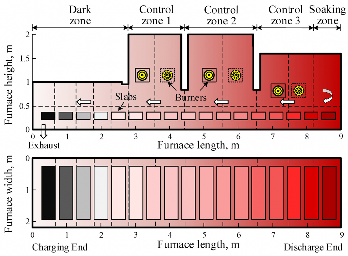
(a)

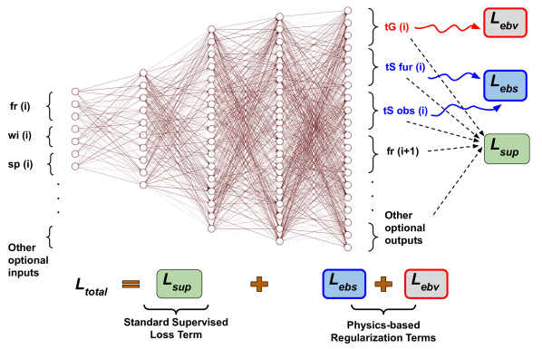
(b)

Figure 1: This figure is best viewed in color. Sub-figure (a) Illustration of a real-world furnace, and its subdivision as different zones. Image courtesy: [8]. A darker shade of red indicates a higher temperature. Under normal conditions, temperature increases towards the discharge end. Sub-figure (b) Illustration of incorporating zone method based regularization to train a Physics-Informed Neural Network (PINN).

1.1 Related works

To the best of our knowledge, our study using the Hottel’s zone method in conjunction with ML, DL, and PINNs, in a regression setup, for the application of temperature prediction in reheating furnaces is a first of its kind and has the potential to open up newer research. However, we now would like to discuss a few works in the literature that are related to (in terms of some theoretical aspects) but are different from our work (for a direct experimental comparison).

Ebrahimi et al. [20] studied zonal modeling of RHT in industrial furnaces. However, their focus was only limited to an approximate exchange area calculation and not temperature prediction in an end-to-end data-driven fashion. As the calculation is very difficult for complex geometries (e.g. by considering radiation interaction between obstacles), they use simplified numerical integration to determine exchange areas. However, our geometry-agnostic approach makes no such simplification and can incorporate an arbitrary enclosure. Our learned neural network directly predicts the temperatures, while their method is focused on exchange area calculation.

Kang [21] proposed a genetic algorithm based method for nonlinear dynamic systems. They attempt to incorporate prior awareness by simplifying the modeling with the assumption that the underlying equations could be approximated with only a fixed set of mathematical operations. These simple operations are directly used as activation functions of neurons. They then make use of an evolutionary approach / genetic algorithm to produce a neural network. Despite their philosophy being similar to modern-day physics-aware neural network based methods, this method is not directly applicable to our use-case of temperature prediction. This is because the underlying physics equations in RHT are based on a different set of operations. We instead let the network learn freely from the data, and ensure generalization and physics awareness by using simple, flexible regularizers.

Yuen [22] focused on using a neural network to calculate absorption coefficients of non-grey/ real gases, but we use several grey gases to represent real gases, i.e., Weighted Sum of the mixed Grey Gases (WSGG) model [8]. Their method is just a different way to calculate the radiation properties of a real gas and is only a subset of RHT as used in our paper, i.e., emissivity (for grey gases). García et al. [23] focused on near-field RHT or close regime, where the assumptions of geometrical optics inherent to classical RHT (that is the case in most industrial applications) are not valid, and can result in heat transfer rates exceeding the blackbody limit of classical RHT. Melot et al. [24] focused on classical RHT problems, but through solving the equation of radiation, which is complex and time-consuming and is avoided in our approach. Tausendschön et al. [25] proposed a neural network based view factor model to compute RHT rates in DEM-based simulations.

2 Proposed Method

In the introduction section, we have discussed the Hottel’s zone method [14, 15, 16] to alleviate the problem of obtaining good quality training data in reheating furnaces for effective temperature prediction via ML. Next, we shall introduce the basics of furnace operation, and then move on to the zone method, followed by a description of how we can utilize the method to generate IID data suitable for training regression-based ML and DL models. For the self-sufficiency of our paper, we will seamlessly integrate the necessary background/s as required. We shall also discuss how one can incorporate physical knowledge of the underlying phenomenon by virtue of our novel regularizers within a neural network to make it physics-informed.

Real-world furnace operation: To illustrate our method and conduct experiments, we shall take as a reference a real-world, walking beam top-fired furnace in Swerim (former Swerea MEFOS), Sweden, which has been studied by Hu et al. [8]. As can be seen in Figure 1(a), the furnace is subdivided into several zones (e.g., dark, control, soaking, etc). It has varying heights for different zones but is of fixed length and width. It has a target heating temperature of 1250 ^∘C and its production capacity is 3 tonne/hr. Reheating furnaces are used to heat intermediate steel products usually known as stock (e.g., blooms, billets, slabs).

Through a series of discrete pushes, the transport of slabs occurs within a furnace. As shown in Figure 1(a), a first slab at an ambient temperature is pushed from the charge end (lower temperature, shown in a lighter shade of red). At each push, all slabs move forward towards the discharge end (higher temperature, shown in a darker shade of red). For a few specific regions in the furnace, the process operator pre-defines a few set point temperatures, which indicate the temperatures to which the slabs must be heated. The slabs once heated to the required set point temperatures, are collected at the discharge end. The movement of the slabs is controlled by the walk-interval (walk rate), depending on the desired throughput.

It should be noted that a furnace usually operates in steady-state equilibrium, and the internal combustion is controlled via firing rates of a few burners located in specific regions. In Figure 1(a), we can see that there are six burners: 2 in each of control zones 1, 2, and 3. In this particular furnace, the pair of burners in a control zone share the same firing rate values. Note that these firing rates are normalized in $[0,1]$.

Entities for temperature prediction: In the above discussion, we have mentioned three important entities: i) set point temperatures, ii) walk interval, and iii) firing rates. With these, and (optionally, per design choice) the initial state of the furnace (indicated by temperatures of various regions in it), as inputs, there would be changes in the mass and energy flow within the furnace, depending on the overall movement of the slabs. This results in a new furnace state, which could be represented by a new, corresponding set of temperatures. Given these discussed inputs, we ideally expect a computational model to predict the next set of corresponding temperatures, which could be matched with the set point temperatures. If the temperature achieved for a region is less compared to the set point, one would like to increase the firing rate for a burner, and in case of a higher temperature achieved, one would prefer to lower the firing rate. The firing rate adjustment is done via a Proportional-Integral-Derivative (PID) controller, while also taking into account the walk interval.

2.1 Proposed data generation methodology for temperature prediction using ML

As shown in Figure 1(a), it is possible to conceptually divide the furnace into 1, 2, and 12 sections across its width, height, and length respectively. This results in a total of 24 volume/gas zones, where gaseous material could reside. These zones can be visualized using the dashed vertical and horizontal lines in the figure.

Additionally, at a time step, there can be 17 slabs inside the furnace, each of which has 6 surfaces, thus, resulting in 102 slab surfaces. With prior knowledge of the 3D structure of our furnace, we computed a total of 76 furnace walls, which could be called furnace surfaces. We can respectively call the 102 slab surfaces as obstacle/ slab surface zones, and the 76 furnace walls as furnace surface zones. Collectively, the obstacle/ slab surface zones and furnace surface zones result in a total of 178 surface zones, which in addition to the volume zones form the basis of utilization of the Hottel’s zone method.

The flow of combustion products within the furnace results in heat release. This causes radiation interchange among all possible pairs of zones: gas to gas, surface to surface, and surface to gas (and vice-versa). The dominating heat transfer mechanism in such processes is Radiative Heat Transfer (RHT), which naturally occurs among the other heat transfer mechanisms: conduction and convection. For each pair of zones, there would be an energy balance, i.e., the amount of energy entering a zone would equal the amount leaving it. To model the RHT, the zone method subdivides an enclosure into a finite number of isothermal volume and surface zones, and applies energy balance to each of them. In our case, for example, we have a total of 202 zones (178 for surfaces and 24 for volumes).

We can model the radiative exchange among any two zones by leveraging underlying governing physical equations, and energy balances. The zone method also employs pre-computed exchange areas (which are general forms of view factors). The main objective is to then compute unknown parameters such as temperatures (of volumes and surfaces), and heat fluxes. This could be done by solving a set of simultaneous equations. We direct the interested reader to [16], for a better perspective of the zone method.

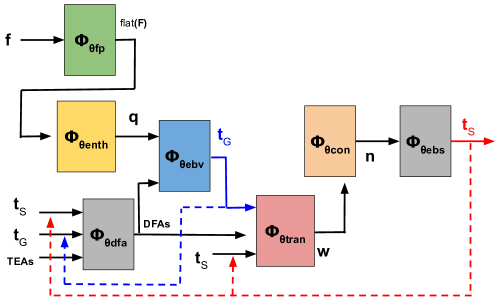
Figure 2: Flow of the proposed zone method based algorithmic approach for ML training data generation. The figure is best viewed in color. Dashed blue/ red backward lines respectively denote that outputs of components ${\boldsymbol{t}}_{G}/{\boldsymbol{t}}_{S}$ (from the previous time-step) are provided as inputs to the current time step.

We shall design the data framework in such a way that it can easily plug in any standard ML (or DL) model for regression. For this, notice that although the various entities within the computational method depend on the geometry of the furnace, we can make a learnable model agnostic of the geometry, if we can train it by simply using data in the form of input-output pairs, and (optional) auxiliary/ intermediate variables (say, for regularization).

One simple way is to collect all relevant values from across zones corresponding to an entity in the form of a vector. For example, we could collect all gas zone temperatures within a vector, and likewise, for other entities such as surface zones, enthalpies, heat fluxes, node temperatures, etc, we could form individual vectors. This gives us the freedom to ignore the 3D structure during training as we can simply deal with vectors and their mappings, say within a neural network, or any other ML technique. Post-inference analysis or fine-grained process control could later be performed via our knowledge of which zone an attribute of the vector maps to.

In Figure 2, we present our proposed algorithmic flow mimicking the Hottel’s zone method [14, 15, 16] based computational model of Hu et al. [17], for data generation aimed at training regression-based ML models. In this, notice how we represent all the relevant entities as vectors. While we shall discuss all relevant terms of the zone method in detail, during the explanation of the modeling part, we now briefly give an overview of the various stages of the zone method. Here, $\Phi$ represents a particular block/ stage, and $\theta$ represents the applicable parameters for the underlying function (abbreviated name shown in the subscript). Following are the stages in the generation method (represented by a block in Figure 2):

1. DFA block ($\Phi_{\theta_{dfa}}$): Notice that for a time step, the inputs ${\boldsymbol{t}}_{S},{\boldsymbol{t}}_{G}$ are obtained from the corresponding values obtained as outputs in the previous time step, shown respectively by dashed red and blue backward arrows. Here, $|S|$ and $|G|$ denote the total number of surface and gas zones, and, ${\boldsymbol{t}}_{S}\in\mathbb{R}^{|S|},{\boldsymbol{t}}_{G}\in\mathbb{R}^{|G|}$ are vectors collecting all the surface zone and gas/volume zone temperatures respectively. Hu et al [17], using an updated Monte-Carlo based Ray-Tracing (MCRT) algorithm [26], provide fixed, pre-computed Total Exchange Areas (TEAs) (forms of view factors [16]) as inputs along with ${\boldsymbol{t}}_{S},{\boldsymbol{t}}_{G}$, for computing the Radiation Exchange factors, or the Directed Flux Area (DFA) terms.

   The TEAs are denoted as: ${\boldsymbol{GS}}\in\mathbb{R}^{|G|\times|S|\times N_{g}}$, ${\boldsymbol{SS}}\in\mathbb{R}^{|S|\times|S|\times N_{g}}$, ${\boldsymbol{GG}}\in\mathbb{R}^{|G|\times|G|\times N_{g}}$, and ${\boldsymbol{SG}}\in\mathbb{R}^{|S|\times|G|\times N_{g}}$ (we can drop the third dimension for the sake of brevity). Here, ${\boldsymbol{GS}}$, ${\boldsymbol{SS}}$, ${\boldsymbol{GG}}$, and ${\boldsymbol{SG}}$ contain the pre-computed gas-surface, surface-surface, gas-gas, and surface-gas exchange areas. $\accentset{\leftharpoonup}{{\boldsymbol{GS}}}\in\mathbb{R}^{|G|\times|S|}$, $\accentset{\leftharpoonup}{{\boldsymbol{SS}}}\in\mathbb{R}^{|S|\times|S|}$, $\accentset{\leftharpoonup}{{\boldsymbol{GG}}}\in\mathbb{R}^{|G|\times|G|}$, and $\accentset{\leftharpoonup}{{\boldsymbol{SG}}}\in\mathbb{R}^{|S|\times|G|}$ are the corresponding DFA terms for ${\boldsymbol{GS}}$, ${\boldsymbol{SS}}$, ${\boldsymbol{GG}}$, and ${\boldsymbol{SG}}$ respectively ($\leftharpoonup$ indicates the direction of flow). Here, $N_{g}$ denotes the number of gases used for representing a real gas medium.

   Initially, we assume that a steady-state has been reached, and hence assign ambient temperature values to ${\boldsymbol{t}}_{S},{\boldsymbol{t}}_{G}$. The parameters $\theta_{dfa}$ represent fixed correlation coefficients (discussed later).

2. Flow pattern ($\Phi_{\theta_{fp}}$) and enthalpy blocks ($\Phi_{\theta_{enth}}$): Given initial firing rates in ${\boldsymbol{f}}\in\mathbb{R}^{|B|}$ ($|B|$ is a function of the number of burners), the block representing the function $\Phi_{\theta_{fp}}$ obtains the flow pattern $flat({\boldsymbol{F}})$, which is further used by the block representing the function $\Phi_{\theta_{enth}}$ to obtain the enthalpy vector ${\boldsymbol{q}}$.

   Note that, the flow of combustion gases within an enclosure causes mass flow into (+ve) and out (-ve) of a zone, for each inter-zone boundary plane. This flow could be pre-computed in a CPU instantly using a polynomial fitted through isothermal CFD simulations that define a range of experimental points, derived with Box–Behnken designs [27]. The flow pattern resulted is by nature a matrix ${\boldsymbol{F}}\in\mathbb{R}^{|G|\times 12}$, but the spatial dependency among the matrix elements can be discarded for simplicity, and we can rather represent an equivalent flattened vector $flat({\boldsymbol{F}})\in\mathbb{R}^{12|G|}$ obtained in row-major fashion. Note that, as already mentioned, we subdivide an enclosure into several cubes/ boxes (zones in our case). Since any cube has 6 surfaces, and for each surface we have two directions of flow (+ve and -ve), this results in 12 flows for each volume zone, and thus, the 12 arises in the dimensionality of ${\boldsymbol{F}}$.

   Also, for each volume zone $i$, we would require an enthalpy transport term $(\dot{Q}_{enth})_{i}$. We introduce an enthalpy vector ${\boldsymbol{q}}\in\mathbb{R}^{|G|}$ to compactly represent these terms.

3. Volume energy balance block ($\Phi_{\theta_{ebv}}$): We introduce a block to compute the volume zone temperatures ${\boldsymbol{t}}_{G}$ using the enthalpy vector ${\boldsymbol{q}}$ and the DFA terms $\accentset{\leftharpoonup}{{\boldsymbol{GG}}}$ and $\accentset{\leftharpoonup}{{\boldsymbol{GS}}}$.

4. Heat transfer block ($\Phi_{\theta_{tran}}$): Together with the volume zone temperatures ${\boldsymbol{t}}_{G}$, the obtained DFAs ($\accentset{\leftharpoonup}{{\boldsymbol{SS}}}$, $\accentset{\leftharpoonup}{{\boldsymbol{SG}}}$), and the previously obtained (or initialized) surface zone temperatures ${\boldsymbol{t}}_{S}$, we obtain the heat transfer/ flux to the surfaces as a variable ${\boldsymbol{w}}$.

5. Conduction analysis block ($\Phi_{\theta_{con}}$): The heat flux on each surface zone serves as a boundary condition for performing a conduction analysis, to compute the transient heat conduction through each surface. The conduction process results in the node temperatures, which we represent as a variable ${\boldsymbol{n}}$.

6. Surface energy balance block ($\Phi_{\theta_{ebs}}$): The computation of heat transfer/ flux and surface zone temperatures are coupled together as the surface energy balance equations. Having computed the heat transfer and performing the conduction analysis, the surface zone temperatures in ${\boldsymbol{t}}_{S}$ can be updated using the node temperatures ${\boldsymbol{n}}$. This is a fixed function.

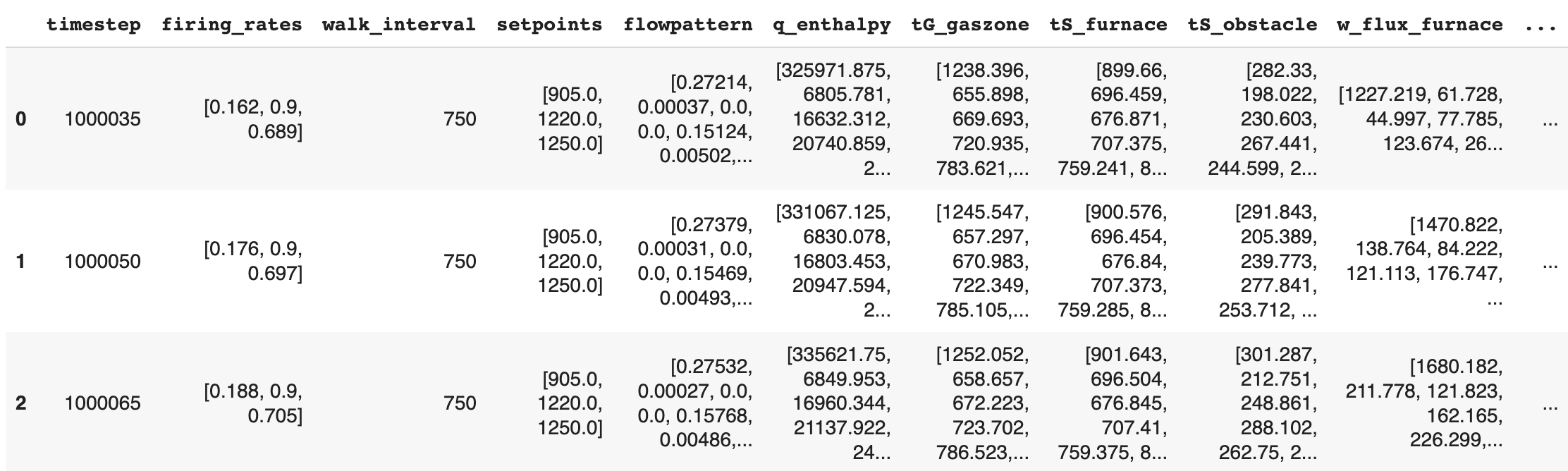
Figure 3: Sample training data instances for each time step within a configuration.

The Algorithm: Algorithm 1 presents the steps involved in the data generation method. We assume that for a steady-state furnace configuration (with fixed set points and walk interval), our data set is in the form: $\mathcal{X}=\{\mathcal{X}_{t}\}_{t=1}^{T}$, where, $\mathcal{X}_{t}=\{{\boldsymbol{f}}^{(t)},{\boldsymbol{F}}^{(t)},{\boldsymbol{q}}^{(t)},{\boldsymbol{t}}_{S}^{(t)},{\boldsymbol{t}}_{G}^{(t)},{\boldsymbol{w}}^{(t)},{\boldsymbol{n}}^{(t)}\}$ is the set of observed variables as described in Figure 2, for a time-step $t$. Note that the computations of flow patterns, enthalpy, and node temperatures can be treated independently from the energy balance equations.

Algorithm 1 Data generation algorithm

1:Initialize a steady-state furnace configuration via set points and walk interval.

2:Initialize $\mathcal{X}=\{\}$, $T>0$ (max no. of steps).

3:Initialize ${\boldsymbol{t}}_{G}^{(0)},{\boldsymbol{t}}_{S}^{(0)}$ with steady-state ambient temperatures, and ${\boldsymbol{f}}^{(0)}$.

4:for t=1 to $T$ do $\triangleright$ t: time-step

5:    ${\boldsymbol{f}}^{(t)}\leftarrow\textrm{update firing rates}({\boldsymbol{f}}^{(t-1)},\textrm{set point temperatures},{\boldsymbol{t}}_{G}^{(t-1)},{\boldsymbol{t}}_{S}^{(t-1)})$

6:    ${\boldsymbol{q}}^{(t)}\leftarrow\Phi_{\theta_{enth}}(\Phi_{\theta_{fp}}({\boldsymbol{f}}^{(t)}))$

7:    $\accentset{\leftharpoonup}{{\boldsymbol{GG}}}^{(t)},\accentset{\leftharpoonup}{{\boldsymbol{GS}}}^{(t)},\accentset{\leftharpoonup}{{\boldsymbol{SG}}}^{(t)},\accentset{\leftharpoonup}{{\boldsymbol{SS}}}^{(t)}\leftarrow\Phi_{\theta_{dfa}}({\boldsymbol{t}}_{G}^{(t-1)},{\boldsymbol{t}}_{S}^{(t-1)},{\boldsymbol{GG}},{\boldsymbol{GS}},{\boldsymbol{SG}},{\boldsymbol{SS}})$

8:    ${\boldsymbol{t}}_{G}^{(t)}\leftarrow\Phi_{\theta_{ebv}}({\boldsymbol{q}}^{(t)},\accentset{\leftharpoonup}{{\boldsymbol{GG}}}^{(t)},\accentset{\leftharpoonup}{{\boldsymbol{GS}}}^{(t)})$

9:    ${\boldsymbol{w}}^{(t)}\leftarrow\Phi_{\theta_{tran}}({\boldsymbol{t}}_{G}^{(t)},{\boldsymbol{t}}_{S}^{(t-1)},\accentset{\leftharpoonup}{{\boldsymbol{SS}}}^{(t)},\accentset{\leftharpoonup}{{\boldsymbol{SG}}}^{(t)})$

10:    ${\boldsymbol{t}}_{S}^{(t)}\leftarrow\Phi_{ebs}(\Phi_{\theta_{con}}({\boldsymbol{w}}^{(t)}))$, ${\boldsymbol{n}}^{(t)}\leftarrow\Phi_{\theta_{con}}({\boldsymbol{w}}^{(t)})$

11:    $\mathcal{X}_{t}\leftarrow\{{\boldsymbol{f}}^{(t)},{\boldsymbol{F}}^{(t)},{\boldsymbol{q}}^{(t)},{\boldsymbol{t}}_{S}^{(t)},{\boldsymbol{t}}_{G}^{(t)},{\boldsymbol{w}}^{(t)},{\boldsymbol{n}}^{(t)}\}$

12:    $\mathcal{X}\leftarrow\mathcal{X}\cup\mathcal{X}_{t}$

13:end for

14:return $\mathcal{X}$

Figure 3 illustrates a few sample time steps (in rows), and the corresponding entities (in columns) generated by using Algorithm 1. The full list of entities that we generate for a time step is: ’timestep’, ’firing_rates’, ’walk_interval’, ’setpoints’, ’flowpattern’, ’q_enthalpy’, ’tG_gaszone’,
’tS_furnace’, ’tS_obstacle’, ’w_flux_furnace’,
’w_flux_obstacle’, ’nodetmp_1d_furnace’,
’nodetmp_2d_obstacle’. The names of the entities are self-explanatory (e.g., ’nodetmp_1d_furnace’ refers to 1D node temperatures for furnace surfaces, ’nodetmp_2d_obstacle’ refers to 2D node temperatures for obstacle surfaces), where G as usual, denotes gas zone and S denotes surface zone, the latter, is further divided into furnace and obstacle. As the temperatures predicted in a time step/ row influence the firing rates for the next time step, there is a time dependency among the rows. However, most standard off-the-shelf ML/ DL models suitable for regression require the data in an Independent and Identically Distributed (IID) format.

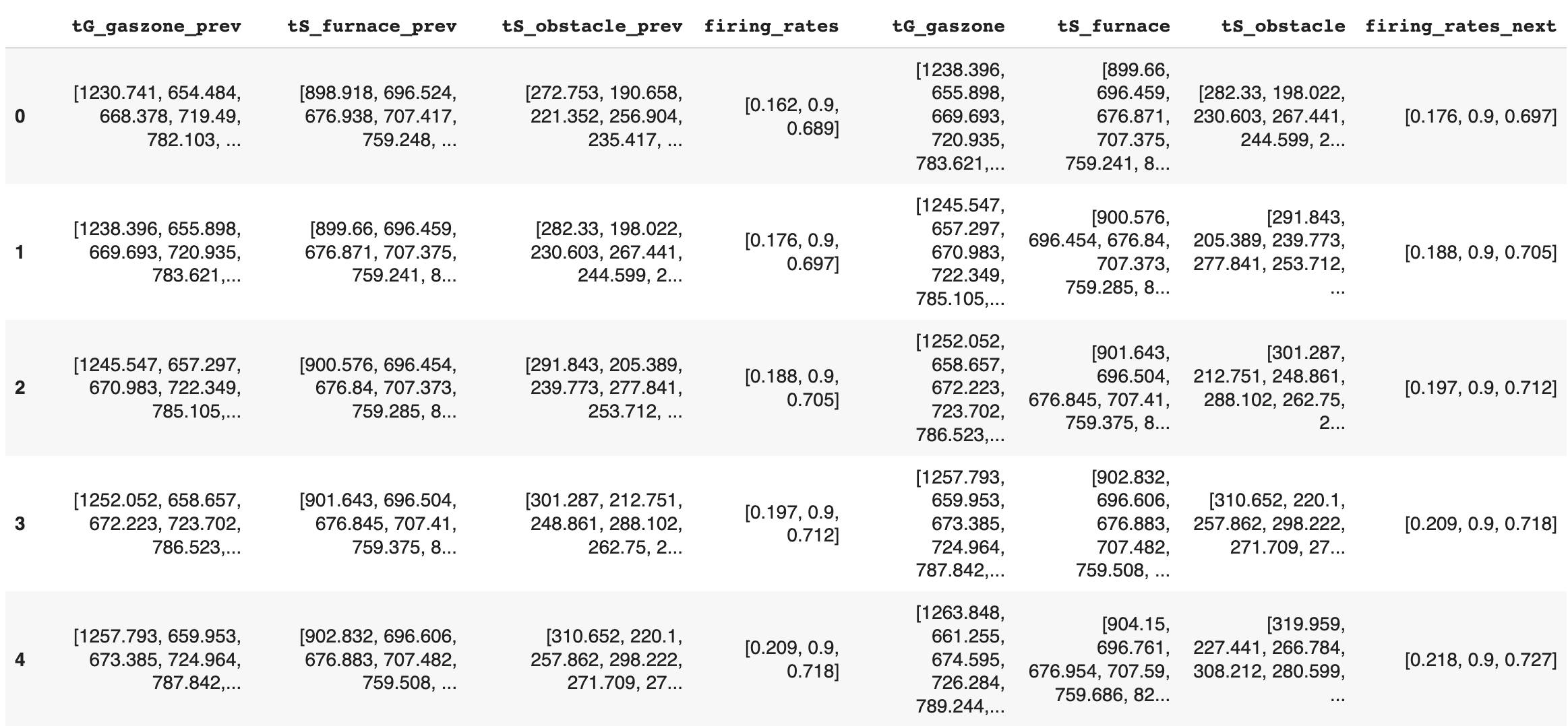
Figure 4: Rearranged training data instances (selected columns).

Assuming that the original time-dependent data is stored in a Pandas DataFrame (using a Python syntax), for each time step we also need the following entities, to obtain IID data: ’firing_rates_next’, ’tG_gaszone_prev’,
’tS_furnace_prev’, and ’tS_obstacle_prev’. This is because, for computing the entities in a time step, we make use of the temperatures in the previous time step. At the same time, for experimental purposes, we also try to directly predict the next firing rate via ML. Thus, using Python syntax, we could perform the following to generate the IID data:
a) df[’firing_rates_next’] = df[’firing_rates’].shift(-1)
followed by df = df.drop(df.tail(1).index).
b) df[’tG_gaszone_prev’]=df[’tG_gaszone’].shift(1),
df[’tS_furnace_prev’] = df[’tS_furnace’].shift(1),
df[’tS_obstacle_prev’] = df[’tS_obstacle’].shift(1)
followed by df = df.drop(df.head(1).index).

The rearranged IID data can be visualized as in Figure 4 (we only showcase relevant entities here, owing to limited space). Essentially, we add a new column ’firing_rates_next’ by shifting the original firing rates column a step back and then dropping the last row. Likewise, we add new columns for prev temperatures by shifting the original temperature columns a step forward and then dropping the first row. Please note that some additional auxiliary variables are used by the computational method of Hu et al. [17], which are mostly constants, and could thus be repeated/ copied for each time step. They are: ’corrcoeff_b’, ’Qconvi’, ’extinctioncoeff_k’, ’gasvolumes_Vi’, ’QfuelQa_sum’,
’surfareas_Ai’, ’emissivity_epsi’,
’convection_flux_qconvi’. We later leverage them in training our PINN, with the help of regularizers.

Now that each row in the table of Figure 4 is IID, we can form any data set containing $N$ IID samples: $\mathcal{X}_{IID}=\{({\boldsymbol{x}}^{(i)},{\boldsymbol{y}}^{(i)})\}_{i=1}^{N}$ to train an off-the-shelf, standard ML/ DL model $f_{\theta}(.)$ with learnable parameters $\theta$, which expects an input instance ${\boldsymbol{x}}^{(i)}$ as vector and predicts an output vector ${\boldsymbol{y}}^{(i)}$, i.e., ${\boldsymbol{y}}^{(i)}=f_{\theta}({\boldsymbol{x}}^{(i)})$. Here, ${\boldsymbol{x}}^{(i)}$ and ${\boldsymbol{y}}^{(i)}$ can be from any of the columns obtained from the rearranged IID table from Figure 4. In our experiments, we study the following two settings for that:

1. Input Setting 1 - Without previous temperatures in the input vector: Here, for time step instance i, we set: ${\boldsymbol{x}}^{(i)}$ = $[fr(i)^{\top},wi(i)^{\top},sp(i)^{\top}]^{\top}$, and
   ${\boldsymbol{y}}^{(i)}$ = $[tG(i)^{\top},tS\textrm{ }fur(i)^{\top},tS\textrm{ }obs(i)^{\top},fr(i+1)^{\top}]^{\top}$.

2. Input Setting 2 - With previous temperatures in the input vector: Here, for time step instance i, we set: ${\boldsymbol{x}}^{(i)}$ = $[fr(i)^{\top},wi(i)^{\top},sp(i)^{\top},tG(i-1)^{\top},tS\textrm{ }fur(i-1)^{\top},tS\textrm{ }obs(i-1)^{\top}]^{\top}$, and
   ${\boldsymbol{y}}^{(i)}$ = $[tG(i)^{\top},tS\textrm{ }fur(i)^{\top},tS\textrm{ }obs(i)^{\top},fr(i+1)^{\top}]^{\top}$.

Here, $fr(i)$, $wi(i)$, $sp(i)$, $tG(i)$, $tS\textrm{ }fur(i)$ and $tS\textrm{ }obs(i)$ are respectively the vectors containing firing rates, walk-interval, set point temperatures, gas zone temperatures, surface zone temperatures for furnace walls, and surface zone temperatures for obstacles for a time step $i$. Also, $tG(i-1)$, $tS\textrm{ }fur(i-1)$, and $tS\textrm{ }obs(i-1)$ are respective vectors containing the corresponding temperatures from the previous time step. Lastly, $fr(i+1)$ is the vector containing the firing rates for the next time step.

In setting 1, merely for an experimental purpose, we avoid the previous temperatures in the inputs to a model. However, we later empirically observe in Tables 7-8 that the performance of any model is better in the setting 2 than the setting 1. This is because setting 2 conforms to the zone method that indeed expects the previous time step temperatures for modeling. Figure 1(b), as used later to illustrate our proposed PINN, shows how the above two input-output settings could be merged generically.

Notice how the above proposed ML training framework via our data generation in the form of simple input-output pairs lets any generic regression model learn freely without requiring 3D geometry-specific knowledge during the training. This makes our proposed framework geometry-agnostic, and hence flexible by nature to accommodate any ML method.

2.2 ML-based temperature prediction

With either of the input settings 1 or 2 as discussed, and a generated dataset of the form $\mathcal{X}_{IID}$=$\{({\boldsymbol{x}}^{(i)},{\boldsymbol{y}}^{(i)})\}_{i=1}^{N}$, we can estimate model parameters $\theta$ using a standard ML/DL technique $f_{\theta}(.)$ by training it to predict ${\boldsymbol{y}}^{(i)}$ given ${\boldsymbol{x}}^{(i)}$, for all $i$. For example, we can train a DL-based Multi-Layer Perceptron (MLP) model as:

$$\theta^{*}\leftarrow\operatorname*{arg\,min}_{\theta}\mathbb{E}_{({\boldsymbol{x}}^{(i)},{\boldsymbol{y}}^{(i)})\in\mathcal{X}_{IID}}[||{\boldsymbol{y}}^{(i)}-f_{\theta}({\boldsymbol{x}}^{(i)})||_{2}^{2}]$$ (1)

Then, we can obtain the required values of temperatures by extracting them from $f_{\theta^{*}}({\boldsymbol{x}}^{(i)})$. We can use a similar procedure to train any standard ML technique, such as Decision Trees, Random Forests, Boosting, etc. We later show the promise of the DL-based MLP, based on a holistic mix of performance and inference efficiency.

2.3 Our proposed physics-informed method

While simulations could sample data at periodic intervals, they are not necessarily able to capture all corner cases. This additionally poses a risk to the Out-Of-Distribution (OOD) generalization capability of the trained DL models, an aspect where DL is not naturally good at [18]. To tackle this, we propose employing a novel Physics-Informed Neural Network (PINN) model [19] based on MLP. This is done via incorporating prior physical knowledge based on the zone method, using a set of our novel proposed Energy-Balance regularizers.

To explain our PINN (see Figure 1(b)), let us use eq(1) and denote: $\mathcal{L}_{sup}=\mathbb{E}_{({\boldsymbol{x}}^{(i)},{\boldsymbol{y}}^{(i)})\in\mathcal{X}_{IID}}[||{\boldsymbol{y}}^{(i)}-f_{\theta}({\boldsymbol{x}}^{(i)})||_{2}^{2}]$ as the standard supervised term. Then, the overall PINN loss is formulated as:

$$\mathcal{L}_{total}=\mathcal{L}_{sup}+\lambda_{ebv}\mathcal{L}_{ebv}+\lambda_{ebs}\mathcal{L}_{ebs}$$ (2)

Here, $\lambda_{ebv},\lambda_{ebs}>0$ are hyper-parameters corresponding to $\mathcal{L}_{ebv}$ and $\mathcal{L}_{ebs}$, such that $\mathcal{L}_{ebv}$=$||\textrm{normalize}({\boldsymbol{v}}_{g})||_{2}^{2}$ is our proposed regularizer term corresponding to the Energy-Balance equations for the Volume zones (EBV) using the zone method. Similarly, $\mathcal{L}_{ebs}$=$||\textrm{normalize}({\boldsymbol{v}}_{s})||_{2}^{2}$ is our proposed regularizer term corresponding to the Energy-Balance equations for the Surface zones (EBS). Normalizing an output vector of a neural network in a regression task is standard practice for ensuring convergence. In our work, we use: $\textrm{normalize}({\boldsymbol{v}})={\boldsymbol{v}}/\textrm{max}({\boldsymbol{v}})$, where $\textrm{max}({\boldsymbol{v}})$ is the maximum value from among all components in ${\boldsymbol{v}}$ (we found it to be better than commonly used sigmoid function based normalization of output). We propose to represent ${\boldsymbol{v}}_{g}$ and ${\boldsymbol{v}}_{s}$ as:

$$\begin{split}&{\boldsymbol{v}}_{g}=({\boldsymbol{g}}_{(g)arr}+{\boldsymbol{s}}_{(g)arr}-4{\boldsymbol{g}}_{leave}+{\boldsymbol{h}}_{g})\in\mathbb{R}^{|G|}\\ &{\boldsymbol{v}}_{s}=({\boldsymbol{s}}_{(s)arr}+{\boldsymbol{g}}_{(s)arr}-{\boldsymbol{s}}_{leave}+{\boldsymbol{h}}_{s})\in\mathbb{R}^{|S|}\end{split}$$ (3)

Intuitively, ${\boldsymbol{v}}_{g}$ and ${\boldsymbol{v}}_{s}$ enforce that the net energy inflow equals the net energy outflow, for respective gas and surface zones, thereby, respecting the Energy-balance equations of the zone method for adhering to the physics of the underlying RHT mechanism.

2.4 Defining the constituting terms in the energy-balance regularizers

Having discussed ${\boldsymbol{v}}_{g}$ and ${\boldsymbol{v}}_{s}$, we now define the terms used to compute them. Let, ${\boldsymbol{g}}_{(g)arr}\in\mathbb{R}^{|G|}$ be a vector whose $i^{th}$ entry represents the amount of radiation arriving at the $i^{th}$ gas zone from all the other gas zones, ${\boldsymbol{s}}_{(g)arr}\in\mathbb{R}^{|G|}$, a vector whose $i^{th}$ entry represents the amount of radiation arriving at the $i^{th}$ gas zone from all the other surface zones, ${\boldsymbol{g}}_{leave}\in\mathbb{R}^{|G|}$, a vector whose $i^{th}$ entry represents the amount of radiation leaving the $i^{th}$ gas zone, and ${\boldsymbol{h}}_{g}\in\mathbb{R}^{|G|}$ a heat term. Also, let $T_{g,j}$ (or $T_{g}$) and $T_{s,j}$ (or $T_{s}$) denote the $j^{th}$ gas and surface zone temperatures respectively. Then, following EBV equations, the $i^{th}$ entries of ${\boldsymbol{g}}_{(g)arr}$, ${\boldsymbol{s}}_{(g)arr}$, ${\boldsymbol{g}}_{leave}$ and ${\boldsymbol{h}}_{g}$ can be computed as:

$${\boldsymbol{g}}_{(g)arr}(i)=\sum_{j}^{|G|}\accentset{\leftharpoonup}{{\boldsymbol{G_{i}G_{j}}}}\sigma T_{g,j}^{4}$$ (4)

$${\boldsymbol{s}}_{(g)arr}(i)=\sum_{j}^{|S|}\accentset{\leftharpoonup}{{\boldsymbol{G_{i}S_{j}}}}\sigma T_{s,j}^{4}$$

$${\boldsymbol{g}}_{leave}(i)=\sum_{n}^{|N_{g}|}a_{g,n}(T_{g,i})k_{g,n}\sigma V_{i}T_{g,i}^{4}$$

$${\boldsymbol{h}}_{g}(i)=-(\dot{Q}_{conv})_{i}+(\dot{Q}_{fuel,net})_{i}+(\dot{Q}_{a})_{i}+{\boldsymbol{q}}_{i}$$

Here, the constants (known apriori) $(\dot{Q}_{conv})_{i}$, $(\dot{Q}_{fuel,net})_{i}$, and $(\dot{Q}_{a})_{i}$ respectively denote the convection heat transfer, heat release due to input fuel, and thermal input from air/ oxygen. An enthalpy vector ${\boldsymbol{q}}\in\mathbb{R}^{|G|}$ is computed using the flow-pattern obtained via polynomial curve fitting during simulation. $\sigma$ is the Stefan-Boltzmann constant, $V_{i}$ is volume of $i^{th}$ gas zone.

Let, ${\boldsymbol{s}}_{(s)arr}\in\mathbb{R}^{|S|}$, be a vector whose $i^{th}$ entry represents the amount of radiation arriving at the $i^{th}$ surface zone from all the other surface zones, ${\boldsymbol{g}}_{(s)arr}\in\mathbb{R}^{|S|}$, a vector whose $i^{th}$ entry represents the amount of radiation arriving at the $i^{th}$ surface zone from all the other gas zones, ${\boldsymbol{s}}_{leave}\in\mathbb{R}^{|S|}$, a vector whose $i^{th}$ entry represents the amount of radiation leaving the $i^{th}$ surface zone, and ${\boldsymbol{h}}_{s}\in\mathbb{R}^{|S|}$ a heat term. Then, following EBS equations, the $i^{th}$ entries of ${\boldsymbol{s}}_{(s)arr}$, ${\boldsymbol{g}}_{(s)arr}$, ${\boldsymbol{s}}_{leave}$ and ${\boldsymbol{h}}_{s}$ can be computed as:

$${\boldsymbol{s}}_{(s)arr}(i)=\sum_{j}^{|S|}\accentset{\leftharpoonup}{{\boldsymbol{S_{i}S_{j}}}}\sigma T_{s,j}^{4}$$ (5)

$${\boldsymbol{g}}_{(s)arr}(i)=\sum_{j}^{|G|}\accentset{\leftharpoonup}{{\boldsymbol{S_{i}G_{j}}}}\sigma T_{g,j}^{4}$$

$${\boldsymbol{s}}_{leave}(i)=A_{i}\epsilon_{i}\sigma T_{s,i}^{4}$$

$${\boldsymbol{h}}_{s}(i)=A_{i}(\dot{q}_{conv})_{i}-\dot{Q}_{s,i}$$

For a surface zone $i$, the constants (known apriori) $A_{i}(\dot{q}_{conv})_{i}$ and $\dot{Q}_{s,i}$ respectively denote the heat flux to the surface by convection and heat transfer from it to the other surfaces. Here, $A_{i}$ is the area, and $\epsilon_{i}$ is the emissivity of the $i^{th}$ surface zone. In eq(4), since the computations are being done for learning the gas zone related terms, the $T_{g}$ terms after being obtained from $f_{\theta}({\boldsymbol{x}})$ (${\boldsymbol{x}}$: input tensor to the PINN) are kept associated with the computational graph for back-propagating, but not the $T_{s}$ terms. The reverse is true in eq(5) where we are learning for the surface zone related terms, i.e., $T_{s}$ terms are kept in the computational graph for back-propagating, but not $T_{g}$ terms.

In addition to the terms explained so far, eq(4) and eq(5) also contain the DFAs and additional terms such as $a_{g,n}(T_{g,i}),k_{g,n}$, which we shall describe next.

2.5 Coefficients and DFA computation

Earlier, we have discussed the notations for the TEA and DFA terms. Now we will discuss the actual computation of the DFAs considering radiating gas medium through a WSGG model [8]. For efficient implementation, we propose a matrix-based reformulation and computations, instead of nested, iterative operations as in the original paper. WSGG is a method used to represent the absorptivity/ emissivity of real combustion products with a mixture of a couple of grey gases plus a clear gas (i.e., the number of grey gases is equal to $N_{g}-1$). Then, the respective gas and surface weighting coefficients $a_{g,n}(T_{g})$ and $a_{s,n}(T_{s})$ are expressed as $N_{g}^{th}$ order polynomials in $T_{g,j}$ and $T_{s,j}$ as follows [8]:

$$a_{g,n}(T_{g,j})=\sum^{N_{g}}_{i=0}b_{i+1,n}T_{g,j}^{i};a_{s,n}(T_{s,j})=\sum^{N_{g}}_{i=0}b_{i+1,n}T_{s,j}^{i}$$ (6)

For each gas indexed by $1\leq n\leq N_{g}$, we have a set of pre-computed correlation coefficients $\{b_{i+1,n}\}_{i=0}^{N_{g}}$, and an absorption/ extinction coefficient $k_{g,n}$. The same coefficients are used for surfaces. Note that in practice, depending on the fuel used (air/oxy), we vary $i$ as $0\leq i\leq L$, where $L\leq N_{g}$. We then propose the following compact matrix forms to collectively represent all DFAs:

$$\accentset{\leftharpoonup}{{\boldsymbol{GS}}}=\sum_{n=1}^{N_{g}}(\overline{GS})_{n}\odot\textrm{broadcast}(\tilde{b}_{n}({\boldsymbol{t}}_{S})^{\top});$$ (7)

$$\accentset{\leftharpoonup}{{\boldsymbol{GG}}}=\sum_{n=1}^{N_{g}}(\overline{GG})_{n}\odot\textrm{broadcast}(\tilde{b}_{n}({\boldsymbol{t}}_{G})^{\top});$$

$$\accentset{\leftharpoonup}{{\boldsymbol{SS}}}=\sum_{n=1}^{N_{g}}(\overline{SS})_{n}\odot\textrm{broadcast}(\tilde{b}_{n}({\boldsymbol{t}}_{S})^{\top});$$

$$\accentset{\leftharpoonup}{{\boldsymbol{SG}}}=\sum_{n=1}^{N_{g}}(\overline{SG})_{n}\odot\textrm{broadcast}(\tilde{b}_{n}({\boldsymbol{t}}_{G})^{\top})$$

Here, ${\boldsymbol{t}}_{S}\in\mathbb{R}^{|S|}$ (${\boldsymbol{t}}_{G}\in\mathbb{R}^{|G|}$) is a vector containing all the surface (gas) zone temperatures, such that its $j^{th}$ entry ${\boldsymbol{t}}_{S}(j)=T_{s,j}$ (${\boldsymbol{t}}_{G}(j)=T_{g,j}$). Taking $\accentset{\leftharpoonup}{{\boldsymbol{GS}}}$ as an example (other three DFAs would follow similarly), $(\overline{GS})_{n}$ is the $n^{th}$ slice of ${\boldsymbol{GS}}$ along the third dimension. Let, ${\boldsymbol{a}}_{n}=\tilde{b}_{n}({\boldsymbol{t}}_{S})$, then $\textrm{broadcast}({\boldsymbol{a}}_{n}^{\top})$ reshapes ${\boldsymbol{a}}_{n}^{\top}$ to the same dimension as $(\overline{GS})_{n}$, i.e., $\mathbb{R}^{|G|\times|S|}$. The $j^{th}$ entry ${\boldsymbol{a}}_{n}(j)$ of ${\boldsymbol{a}}_{n}\in\mathbb{R}^{|S|}$ is computed using the function $\tilde{b}_{n}$ with the correlation coefficients $\{b_{i+1,n}\}_{i=0}^{N_{g}}$ as the parameters, and by following (6).

Table 1: Dataset details. A total of 50 configurations have been used which are categorized as normal or abnormal.

Normal Behaviour Configurations (SP1<SP2<SP3)
Type 1 (Varying SP1 only)	Type 2 (Varying SP2 only)	Type 3 (Varying SP3 only)	Type 4 (Varying WI only)
905_1220_1250_750.csv (Training) 915_1220_1250_750.csv (Val) 925_1220_1250_750.csv 935_1220_1250_750.csv (Training) 945_1220_1250_750.csv (Val) 965_1220_1250_750.csv 975_1220_1250_750.csv (Training) 985_1220_1250_750.csv (Val) 995_1220_1250_750.csv	955_1170_1250_750.csv (Training) 955_1180_1250_750.csv (Val) 955_1190_1250_750.csv 955_1200_1250_750.csv (Training) 955_1210_1250_750.csv (Val) 955_1230_1250_750.csv 955_1240_1250_750.csv (Training)	955_1220_1230_750.csv (Training) 955_1220_1240_750.csv (Val) 955_1220_1250_750.csv 955_1220_1260_750.csv (Training) 955_1220_1270_750.csv (Val) 955_1220_1280_750.csv 955_1220_1290_750.csv (Training) 955_1220_1300_750.csv	955_1220_1250_675.csv (Training) 955_1220_1250_690.csv (Val) 955_1220_1250_705.csv 955_1220_1250_720.csv (Training) 955_1220_1250_735.csv (Val) 955_1220_1250_765.csv 955_1220_1250_780.csv (Training) 955_1220_1250_795.csv (Val) 955_1220_1250_810.csv 955_1220_1250_825.csv (Training)
Abnormal Behaviour Configurations/ Arbitrary SPs
Type 1 (start@955-incr-dec/const)	Type 2 (start@1220-incr-dec)	Type 3 (start@1220-dec-inc)	Type 4 (start@1250-dec-inc)	Type 5 (start@1250-dec-inc)
955_1220_1200_750.csv (Training) 955_1220_1210_750.csv (Val) 955_1220_1220_750.csv 955_1250_1220_750.csv (Training) 955_1250_1220_765.csv (Val) 955_1250_1250_750.csv 955_1260_1250_750.csv (Training) 955_1270_1250_750.csv	1220_1250_955_750.csv (Training) 1220_1250_955_795.csv	1220_955_1250_750.csv (Training) 1220_955_1250_780.csv	1250_955_1220_750.csv (Training) 1250_955_1220_825.csv	1250_1220_955_750.csv (Training) 1250_1220_955_810.csv

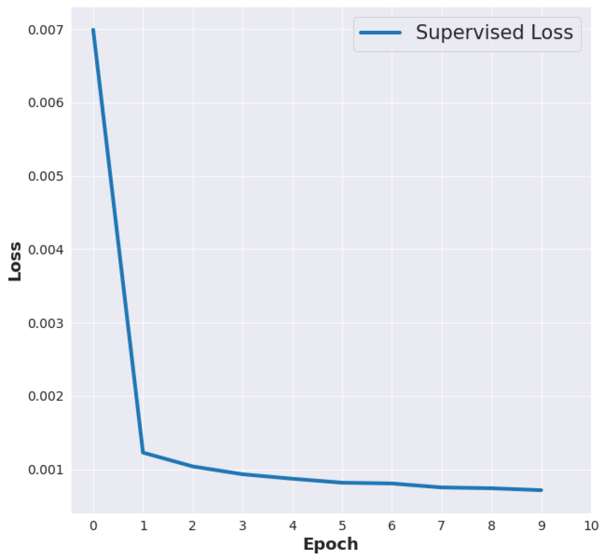
(a)

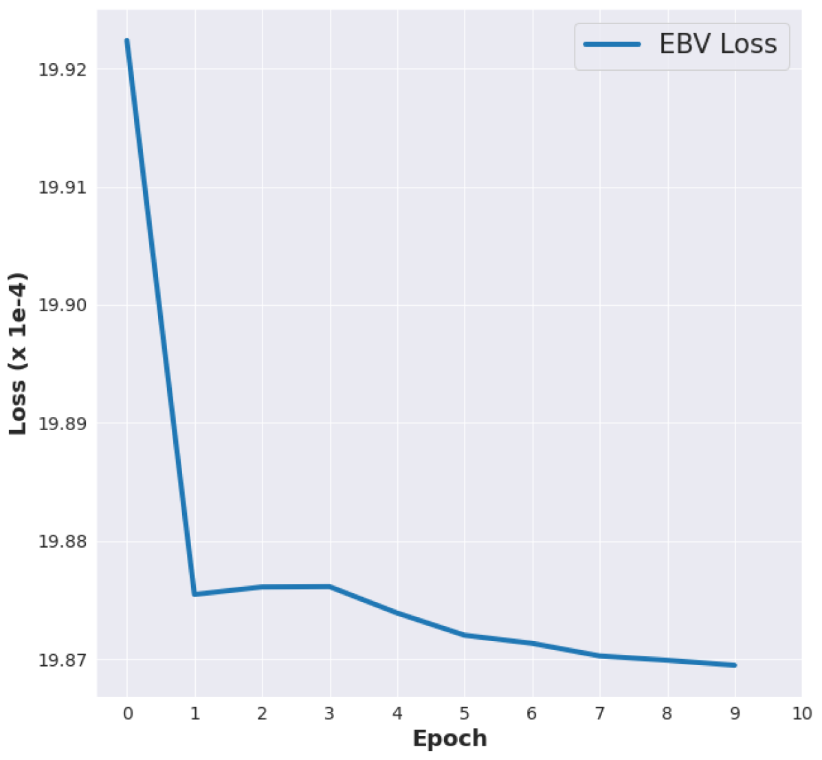
(b)

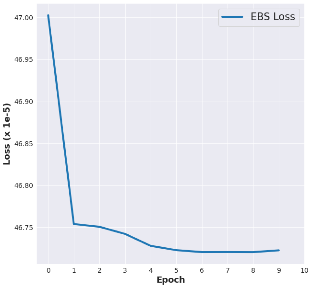
(c)

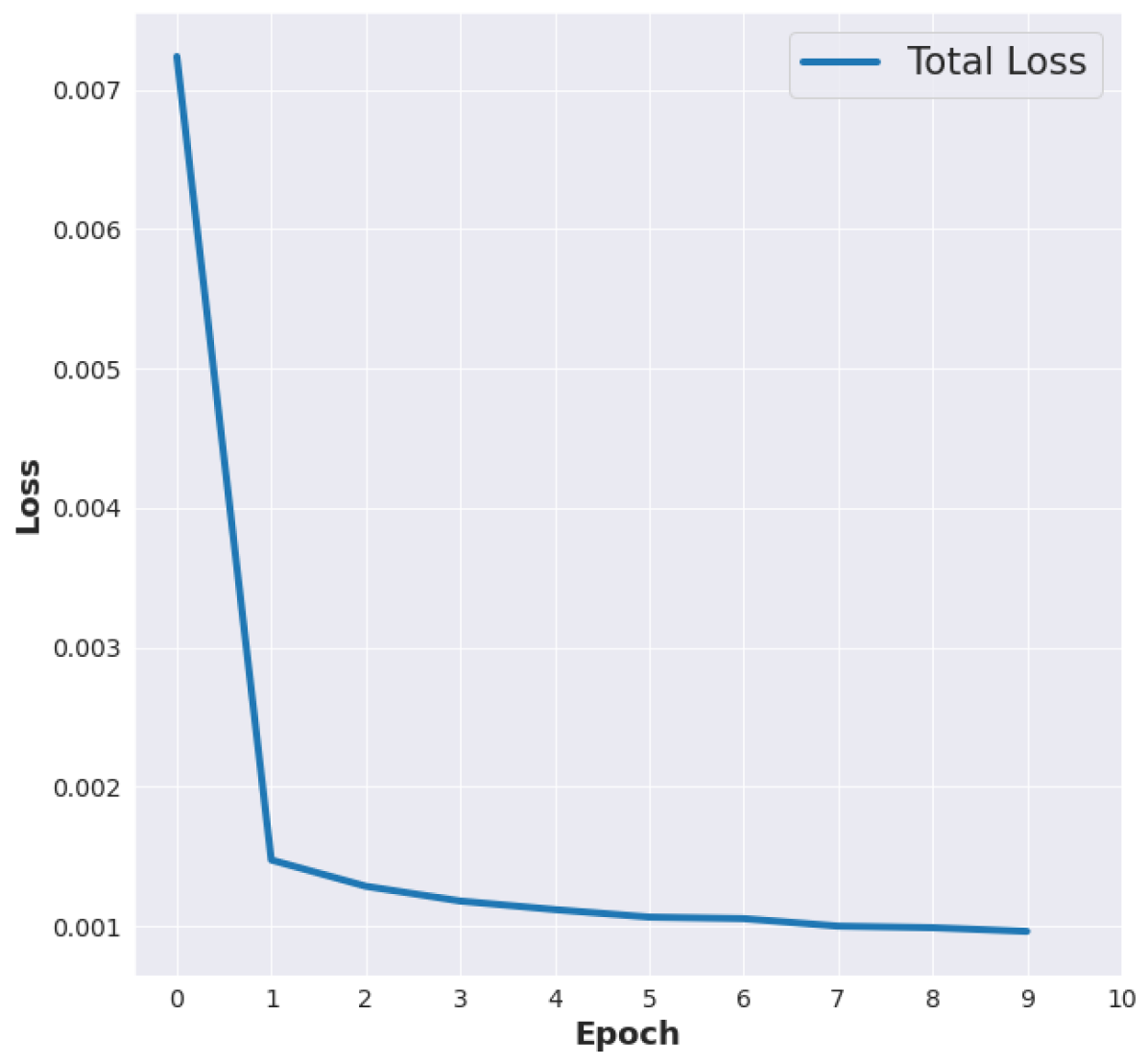
(d)

Figure 5: Convergence behaviour of our method, considering: a) Supervised loss term, b) EBV term, c) EBS term, and d) Total sum of all losses.

3 Experimental Results

3.1 Evaluation protocol

Dataset: Earlier, we have discussed our proposed data generation procedure for training a regression-based ML model with the real-world, walking beam top-fired furnace in Swerim (former Swerea MEFOS), Sweden, shown in Figure 1(a), as an example. A unique steady-state furnace can be configured/ defined by varying the 3 set point temperatures, and the walk interval. We generated data from 50 different configurations (representing a steady-state). Table 1 highlights the details of all the 50 configurations, along with disjoint (to avoid data leakage) train-val-test splits creation.

We represent a configuration as: SP1_SP2_SP3_WI, where SP1, SP2, SP3 and WI respectively denote the set point 1, set point 2, set point 3, and walk interval. Note that we consider configurations with both normal conditions (SP1<SP2<SP3, as naturally occurring in practice), as well as abnormal ones (arbitrary set points). For each configuration, we considered 1500 time steps (at intervals of 15 seconds, to account for the bottleneck conduction analysis step), each of which produces the various physical entities as discussed in Fig 3.

As already discussed, the rearranged IID data can be visualized in Fig 4, and we study both the settings for our experiments: Input Setting 1 - Without previous temperatures in the input vector and Input Setting 2 - With previous temperatures in the input vector. After rearranging the data as IID, we consolidate all the 20 training, 12 validation, and 18 test configurations (with 1500 minus 2 time steps per configuration), resulting in 29960 train, 17976 val, and 26964 test time steps/ IID samples. The 2 time steps are subtracted to account for the shift operations discussed during the IID data creation as mentioned earlier.

Compared methods: Having obtained the IID dataset, and defining the evaluation input settings 1 and 2 for regression, we now study various ML and DL methods to compare their temperature prediction performances via regression. The following methods are compared: i) Decision Tree (DT), ii) Random Forest (RF), iii) Histogram Gradient Boosting (H-GBoost), iv) Multi-Layer Perceptron (MLP), and v) Our proposed Physics-Informed method based on the same architecture as the baseline MLP, but with added EBV and EBS based regularizers (we denote our method as EBV+EBS). The last two methods belong to the category of DL, whereas the remaining are standard classical ML methods, widely chosen for their performance merits, while being representatives of different ML paradigms, for example, ensemble learning and boosting.

All methods are tuned to yield their respective best performance. Experiments were repeated in both GPU and CPU with different seeds, and upon averaging, the trends were observed to be consistent despite the hardware. We use random search for hyper-parameter tuning by taking feedback from validation data and evaluating model performances on test data. As standard recommended practice for ensuring training convergence in regression via neural networks, we need to normalize inputs and outputs to $[0,1]$ (in our case, inputs already are normalized by the computational model).

Performance metrics: For a data set containing $N$ IID samples: $\mathcal{X}_{IID}=\{({\boldsymbol{x}}^{(i)},{\boldsymbol{y}}^{(i)})\}_{i=1}^{N}$, we make use of the following standard regression performance evaluation metrics:

1. Root Mean Squared Error (RMSE), defined as:

   $$RMSE=\sqrt{\frac{\sum_{i=1}^{N}({\boldsymbol{y}}^{(i)}-f_{\theta}({\boldsymbol{x}}^{(i)}))^{2}}{N}}$$ (8)

2. Mean Absolute Error (MAE), defined as:

   $$MAE=\frac{\sum_{i=1}^{N}\left|{\boldsymbol{y}}^{(i)}-f_{\theta}({\boldsymbol{x}}^{(i)})\right|}{N}$$ (9)

3. Coefficient of determination ($R^{2}$), defined as:

   $$R^{2}=1-\frac{\sum_{i=1}^{N}({\boldsymbol{y}}^{(i)}-f_{\theta}({\boldsymbol{x}}^{(i)}))^{2}}{\sum_{i=1}^{N}({\boldsymbol{y}}^{(i)}-\bar{{\boldsymbol{y}}}^{(i)})^{2}}$$ (10)

In the $R^{2}$ computation, $\bar{{\boldsymbol{y}}}^{(i)}$ denotes the average value of the ground truths. We compare model performances for each of the following entities separately: tG, tS fur, and tS obs, respectively denoting the standard terms as described earlier, i.e., gas zone temperatures, furnace surface temperatures, and obstacle surface temperatures. For each of the compared entities, we can compute the performance metrics only by considering their corresponding predictions extracted from ($f_{\theta}({\boldsymbol{x}}^{(i)})$) and ground truth values extracted from (${\boldsymbol{y}}^{(i)}$).

As seen later, in the tables showing the empirical results, we compute the metrics individually for each of the relevant entities as follows: RMSE tG, RMSE tS fur, RMSE tS obs, MAE tG, MAE tS fur, MAE tS obs, $R^{2}$ tG, $R^{2}$ tS fur, $R^{2}$ tS obs, and mMAPE fr. For all tables, the results are on the test split, as is the standard. A lower value of RMSE, MAE, and mMAPE indicates a better performance (indicated by $\downarrow$ in the results tables), while a higher value of $R^{2}$ indicates a better performance (indicated by $\uparrow$ in the results tables). $R^{2}$ ranges between 0 and 1, RMSE and MAE ranges in $[0,\infty]$.

Using the Mean Absolute Percentage Error (MAPE) metric for evaluating the performance of firing rate prediction, as typically used in evaluating forecasting methods, could lead to division by zero as firing rates are close to zero. So, we add $\epsilon>0$ to the denominator of the MAPE computation, and call this a modified MAPE (mMAPE), computed as follows:

$${\footnotesize mMAPE=\frac{1}{N}\sum_{t=1}^{N}\left|\frac{f_{t}-\hat{f}_{t}}{f_{t}+\epsilon}\right|}$$ (11)

Here, $f_{t}$ is the actual firing rate, and $\hat{f}_{t}$ is the predicted value. Table 4 gives an idea of how the $mMAPE$ changes by varying $\epsilon$, taking a naive baseline’s performance on the test split in the IID setting (as discussed later). By setting a very small value of $\epsilon$ we do not change the variables too much, and at the same time, the scores get scaled, to observe larger differences among various methods compared. For all experiments, we set $\epsilon=0.05$. A lower mMAPE indicates a better performance and is evaluated only for the firing rates.

Table 2: Effect of $\epsilon$ on
mMAPE using
Naive Avg.

$\epsilon$	mMAPE
0.05	155.30
0.5	24.94
1	14.44
5	3.56
10	1.85
100	0.19

Table 3: Performance of EBV+EBS (ReLU) variant of our method
against varying hidden layer configurations.

Metric/ Hidden layer configuration	[100]	[50,100]	[50,100, 200]	[50,100, 200,200]	[50,100, 200,200, 205,205]
RMSE tG ($\downarrow$)	11.64	17.25	10.04	10.84	14.27
RMSE tS fur ($\downarrow$)	10.05	15.23	7.95	7.83	12.46
RMSE tS obs ($\downarrow$)	34.82	37.62	31.64	33.57	36.42
mMAPE fr ($\downarrow$)	8.76	9.15	6.84	8.06	7.51

Table 4: Performance of the proposed EBV+EBS
variant using different batch sizes.

Metric	EBV+EBS ReLU bsz=32	EBV+EBS ReLU bsz=64	EBV+EBS ReLU bsz=128
RMSE tG ($\downarrow$)	12.70	10.04	10.73
RMSE tS fur ($\downarrow$)	9.14	7.95	9.69
RMSE tS obs ($\downarrow$)	39.75	31.64	31.79
mMAPE fr ($\downarrow$)	5.24	6.84	8.29

Table 5: Effect of individual regularizer terms in our
method.

Metric	EBV only	EBS only	EBV+EBS
RMSE tG ($\downarrow$)	11.85	11.66	10.04
RMSE tS fur ($\downarrow$)	10.36	11.07	7.95
RMSE tS obs ($\downarrow$)	32.46	32.04	31.64
mMAPE fr ($\downarrow$)	6.42	7.53	6.84

Table 6: Performance of our method using different activation functions in the
underlying network.

Metric	EBV+EBS ReLU	EBV+EBS GeLU	EBV+EBS SiLU	EBV+EBS Hardswish	EBV+EBS Mish
RMSE tG ($\downarrow$)	10.04	13.57	10.07	15.26	10.16
RMSE tS fur ($\downarrow$)	7.95	8.86	8.02	14.02	7.71
RMSE tS obs ($\downarrow$)	31.64	39.65	31.64	36.23	31.63
mMAPE fr ($\downarrow$)	6.84	5.88	6.23	7.03	6.33

Table 7: Comparison of our proposed method against naive baseline and MLP without physics-based regularizer, in an IID evaluation setting.

Without previous temperatures as inputs
	Baseline Methods		Proposed Physics-Informed Method
Performance Metric	Naive Avg	MLP Baseline	EBV+EBS
RMSE tG ($\downarrow$)	58.63	10.27	10.04
RMSE tS fur ($\downarrow$)	53.03	8.94	7.95
RMSE tS obs ($\downarrow$)	68.19	30.94	31.64
MAE tG ($\downarrow$)	39.04	7.31	7.19
MAE tS fur ($\downarrow$)	34.45	5.97	5.58
MAE tS obs ($\downarrow$)	42.27	14.95	15.13
$R^{2}$ tG ($\uparrow$)	-0.031	0.954	0.961
$R^{2}$ tS fur ($\uparrow$)	-0.042	0.948	0.959
$R^{2}$ tS obs ($\uparrow$)	-0.065	0.886	0.885
mMAPE fr ($\downarrow$)	155.30	7.41	6.84
With previous temperatures as inputs
	Baseline Methods		Proposed Physics-Informed Method
Performance Metric	Naive Avg	MLP Baseline	EBV+EBS
RMSE tG ($\downarrow$)	58.63	5.75	4.91
RMSE tS fur ($\downarrow$)	53.03	4.77	4.24
RMSE tS obs ($\downarrow$)	68.19	17.18	17.39
MAE tG ($\downarrow$)	39.04	3.21	3.01
MAE tS fur ($\downarrow$)	34.45	3.09	2.74
MAE tS obs ($\downarrow$)	42.27	4.80	5.81
$R^{2}$ tG ($\uparrow$)	-0.031	0.984	0.989
$R^{2}$ tS fur ($\uparrow$)	-0.042	0.983	0.989
$R^{2}$ tS obs ($\uparrow$)	-0.065	0.966	0.966
mMAPE fr ($\downarrow$)	155.30	7.86	6.87

Table 8: Comparison of our proposed method against classical ML baselines, in an IID evaluation setting.

Without previous temperatures as inputs
	Classical ML Baselines			Proposed Physics-Informed Method
Performance Metric	DT	RF	H-GBoost	EBV+EBS
RMSE tG ($\downarrow$)	12.84	12.24	14.06	10.04
RMSE tS fur ($\downarrow$)	9.42	8.97	10.09	7.95
RMSE tS obs ($\downarrow$)	42.86	42.06	42.73	31.64
MAE tG ($\downarrow$)	8.32	8.02	8.24	7.19
MAE tS fur ($\downarrow$)	6.19	6.01	6.28	5.58
MAE tS obs ($\downarrow$)	17.97	17.72	18.00	15.13
$R^{2}$ tG ($\uparrow$)	0.943	0.948	0.925	0.961
$R^{2}$ tS fur ($\uparrow$)	0.951	0.957	0.934	0.959
$R^{2}$ tS obs ($\uparrow$)	0.788	0.798	0.763	0.885
mMAPE fr ($\downarrow$)	5.50	5.30	2.32	6.84
With previous temperatures as inputs
	Classical ML Baselines			Proposed Physics-Informed Method
Performance Metric	DT	RF	H-GBoost	EBV+EBS
RMSE tG ($\downarrow$)	11.17	6.96	5.00	4.91
RMSE tS fur ($\downarrow$)	10.24	6.15	6.12	4.24
RMSE tS obs ($\downarrow$)	43.05	32.81	23.01	17.39
MAE tG ($\downarrow$)	6.20	4.04	2.31	3.01
MAE tS fur ($\downarrow$)	5.78	3.64	2.70	2.74
MAE tS obs ($\downarrow$)	13.55	9.97	4.01	5.81
$R^{2}$ tG ($\uparrow$)	0.925	0.979	0.989	0.989
$R^{2}$ tS fur ($\uparrow$)	0.915	0.977	0.983	0.989
$R^{2}$ tS obs ($\uparrow$)	0.729	0.890	0.937	0.966
mMAPE fr ($\downarrow$)	6.98	8.09	0.76	6.87

Table 9: Comparison of our proposed method against MLP without physics-based regularizer, in an auto-regressive evaluation setting.

Without previous temperatures as inputs
Metric/ Method	MLP	EBV+EBS	EBV+EBS improvement over MLP (in %)
RMSE tG ($\downarrow$)	28.6	27.3	4.2
RMSE tS fur ($\downarrow$)	10.1	9.6	4.8
RMSE tS obs ($\downarrow$)	42.7	44.0	-3.1
MAE tG ($\downarrow$)	17.1	16.1	5.8
MAE tS fur ($\downarrow$)	7.8	7.3	6.5
MAE tS obs ($\downarrow$)	20.0	20.2	-1.1
mMAPE fr ($\downarrow$)	69.2	63.5	8.2
With previous temperatures as inputs
Metric/ Method	MLP	EBV+EBS	EBV+EBS improvement over MLP (in %)
RMSE tG ($\downarrow$)	74.1	36.8	50.3
RMSE tS fur ($\downarrow$)	74.5	25.8	65.4
RMSE tS obs ($\downarrow$)	83.3	65.3	21.5
MAE tG ($\downarrow$)	48.8	29.3	39.9
MAE tS fur ($\downarrow$)	49.7	20.8	58.2
MAE tS obs ($\downarrow$)	53.6	42.0	21.6
mMAPE fr ($\downarrow$)	96.2	40.6	57.8

3.2 In-depth understanding of our proposed PINN method EBV+EBS

Default setting of our method: We train our PINN model EBV+EBS for 10 epochs using PyTorch, with early stopping to avoid over-fitting. For our method, in an EB equation, certain terms (e.g., enthalpy, flux, temperatures) take large values in the order of hundreds or thousands. Thus, to avoid gradient explosions/ loss divergence during training, we perform the dividing by the max value normalization as in the final neural network output (discussed earlier).

We found a learning rate of 0.001 with Adam optimizer and batch size of 64 to be optimal, along with ReLU non-linearity. We pick the [50,100,200] configuration for hidden layers, i.e., 3 hidden layers, with 50, 100, and 200 neurons respectively. We use $\lambda_{ebv}=\lambda_{ebs}=0.1$. In general, a value lesser than 1 is observed to be better, otherwise, the model focuses less on the primary temperature prediction task. Following are values of other variables: $|G|=24$, $|S|=178$ (76 furnace surface zones and 102 obstacle surface zones), $N_{g}=6$, and Stefan-Boltzmann constant=5.6687e-08. Unless otherwise stated, this is the setting we use to report any results for our method, for example, while comparing with other methods.

Next, to study our PINN in detail, we now vary different aspects of our method (e.g., the impact of individual loss/regularization terms, hidden layer configuration, batch size, and activation functions). At a time, we vary one focused aspect, and fix all other hyper-parameters as per the default setting prescribed above.

Empirical convergence of our method: Firstly, we study the empirical convergence of the default setting of our method. Fig 5 plots the convergence behaviour of each of the loss terms individually (supervised term, EBV term, and EBS term), as well as the total loss. Our method, as shown, enjoys a good convergence both in terms of individual losses, as well as the total loss.

Effect of the hidden layer configuration: In Table 4, we report the performance of our method by varying the hidden layer configurations (e.g., $[100]$ denotes one hidden layer with 100 neurons, $[50,100]$ denotes two hidden layers with 50, and 100 neurons respectively, and so forth). The maximum values for each row (corresponding to a metric) are shown in bold. We found that it suffices to use [50, 100, 200] configuration for a competitive performance.

Effect of batch size: In Table 4, we vary the batch size in our method. We found a batch size of 64 to provide an optimal performance for our experiments.

Effect of individual regularization terms: In Table 6, we study the effect of individual physics-based regularization terms used in our method. We found that using both instances of volume and surface zone based regularizers together leads to better performance as compared to either EBV or EBS in isolation.

Effect of activation functions: In Table 6, we vary the underlying activation functions in our model. While we observed the benefits of using ReLU, SiLU, and Mish over others, there is no clear winner. All three lead to competitive performance. But when it comes to consistent performance across batch sizes, we noticed from our experiments that ReLU is more robust. Thus, we could recommend using the basic ReLU as de facto in our experiments.

3.3 Comparing our proposed PINN with DL-based MLP and the naive baseline

In Table 7 we compare our PINN method (EBV+EBS) against a DL-based MLP neural network that has the same architecture and training setting/ configuration as ours, except the physics-based regularizers. We also compare against the naive baseline, i.e., the one that simply predicts the average value from the training data, corresponding to each output variable.

We report the performance for the two settings as discussed earlier (input settings 1 and 2), i.e., without and with the previous temperatures as inputs to the models. Because of additional supervisory signals about the previous state of a furnace, the case with previous temperatures as inputs leads to lower errors (better performance), for all learning-based techniques (except the naive baseline where performance would remain the same). The DL-based MLP outperforms the naive baseline, indicating that the data-driven training is indeed learning towards a better solution. However, our proposed method by virtue of the physics-based regularizers, which is the only difference against the MLP, outperforms the latter, overall.

3.4 Comparing our proposed PINN with classical ML baselines

In addition to DL, we also compare our method against the classical ML baselines: i) Decision Tree (DT), ii) Random Forest (RF), and iii) Histogram Gradient Boosting (H-GBoost). When it comes to only the classical ML baselines, the performances are as per the expectation. For instance, with previous temperatures as inputs, the performance of DT, RF, and H-GBoost increases. However, being an ensemble learning method, RF performs superior to DT. At the same time, by virtue of boosting, among all the three classical methods, H-GBoost performs the best.

We observe superior performance of our model against the classical baselines as well, as reported in Table 8. In this particular case, DL-based methods (MLP, and our EBV+EBS) perform better than the classical ML ones on average. H-GBoost, though competitive, is very slow for multi-output regression (takes $\sim$ 15 minutes for inferring on 26964 test samples, in contrast to a few milliseconds by neural network methods like MLP and EBV+EBS). This makes it unsuitable for real-world deployment in our particular use case of temperature prediction in reheating furnaces (though it has its merits in other data science applications).

3.5 Auto-regressive evaluation

Having demonstrated various in-depth studies of our proposed PINN method, and its comparison against representative DL and ML baselines by following an IID evaluation setup, we now conduct experiments on another setting, which we refer to as the auto-regressive evaluation setting. This is similar to the real operating condition of an industrial furnace during deployment. Here, we train a model exactly similar to the IID setting (using the train-val splits) but evaluate using a different protocol on the test split. The training has to be the same as IID because the ML/DL models expect the data to be IID. However, during testing, instead of mixing the rows from across all furnace configurations in an IID manner, we evaluate the model performance on each furnace individually, but auto-regressively.

Once we get a model checkpoint using the training data, for evaluating a furnace configuration, we initialize the starting firing rates and let the model infer on the very first time step/ row to predict the temperatures and the next firing rates. These are then used as inputs to the model to make further predictions in the next time step and iterate this over the entire furnace configuration. This is different from the IID setting where a time step/ row would be provided with the actual (correct) inputs obtained during data generation. This makes the auto-regressive setting relatively tougher than the IID setting. For performance metric evaluation, we have the ground truth values and the predictions for each time step, and we can simply compare the average performance across each time step for the data of the furnace configuration in evaluation. The metric evaluation is thus the same as the IID setting.

We use this setting and compare the performance of the two DL-based methods, i.e., our method EBV+EBS, against the baseline MLP (next best method observed from Tables 7-8). In the auto-regressive evaluation setting, we expect that the performance of a model would degrade, compared to the numbers seen in earlier tables. This is verified by the higher error values in Table 9, vs Tables 7-8. For reporting the auto-regressive results in Table 9, we first compute the average performance metric across all rows (evaluated sequentially), for a furnace. Then, the average across all the test furnace configurations is reported in the table.

For input setting 1 (without previous temperatures as inputs), we observed consistently better performance of our method, which is by virtue of the physics-based regularizers. By looking at the columns named EBV+EBS improvement over MLP (in %), we could see that our PINN method obtains up to 8.2% better performance over the baseline MLP (for next firing rates prediction). For obstacle surfaces, the PINN encounters a slight drop of 1% in terms of the MAE. However, for the gas zone and furnace surfaces, the PINN achieves $\sim$6% better MAE than the MLP without physical knowledge.

When we further provide previous temperatures as inputs (i.e., setting 2), cumulative error propagation via an increased number of auto-regressively obtained inputs leads to further performance degradation for both methods. That is why in Table 9, compared to the numbers for the section Without previous temperatures as inputs, the numbers for the section With previous temperatures as inputs would see a further drop. However, interestingly, when previous temperatures are provided as inputs, which is the most challenging setting of all, the performance of the MLP deteriorates significantly. This might be because it merely learns to memorize the training data, without really understanding the underlying physical phenomenon. On the other hand, our method, being aware of the underlying physics, is more generalizable and hence performs significantly better than the MLP baseline (up to 50-65% improvements). The gains achieved by the PINN in this case are consistent for gas zones, furnace surfaces, and obstacle surfaces.

4 Conclusion and future work

In our paper, we studied the problem of effective and efficient temperature prediction in reheating furnaces, with the larger aim of achieving Net-Zero goals in foundation industries. To do this, we suggest relying on computational models. However, due to computational efficiency concerns, existing surrogate models are not suitable for real-world deployment, and as such, we propose using Machine Learning (ML) and Deep Learning (DL) based techniques. Due to the infeasibility of achieving good quality data in the studied scenarios, classical Hottel’s zone method based computational model has been used to generate data for ML and DL-based model training via regression.

Extensive comparison among a wide range of state-of-the-art, representative ML and DL methods (Decision Trees, Random Forests, Boosting, Multi-Layer Perceptron) has been done to use this data and predict furnace temperatures in unknown environments. The promise of DL has been showcased, taking into account a holistic balance between inference times and model performance. To further enhance the Out-Of-Distribution (OOD) generalization capability of the trained DL models, we propose a Physics-Informed Neural Network (PINN) by incorporating prior physical knowledge using a set of novel Energy-Balance regularizers. Our setup being a generic framework, is geometry-agnostic of the 3D structure of the underlying furnace, and as such could accommodate any standard ML regression model.

To the best of our knowledge, our work for the first time proposes a geometry-agnostic ML reformulation of the temperature prediction problem in industrial heating systems such as furnaces, via the zone method. With our proposed data generation, we study both IID and auto-regressive settings of evaluating models. The proposed regularizers clearly demonstrate a better performance over a neural network without physical knowledge, in all settings studied in the paper.

Currently, we have to train all models in an IID setting, due to their inherent nature. A future work could be studied, where we train a physics-aware network based on Recurrent Neural Networks (RNNs) and Back-Propagation through Time (BPT), for directly capturing time dependencies during training. Another avenue of exploration would be to leverage a Reinforcement Learning (RL) or Graph-based physics-aware hybrid for incorporating additional, pluggable PID logic for firing rate updation. Dynamically updating the TEAs could also be a possible direction for exploration.

References

- EPSRC report [2020] EPSRC report, EPSRC report, https://gow.epsrc.ukri.org/NGBOViewGrant.aspx?GrantRef=EP/V026402/1, 2020.
- IOM3 report [2023] IOM3 report, IOM3 report, https://www.iom3.org/resource/transforming-foundations-industries.html, 2023.
- Zhang et al. [2018] Q. Zhang, J. Xu, Y. Wang, A. Hasanbeigi, W. Zhang, H. Lu, M. Arens, Comprehensive assessment of energy conservation and co2 emissions mitigation in china’s iron and steel industry based on dynamic material flows, Applied Energy 209 (2018) 251–265.
- Liang et al. [2020] T. Liang, S. Wang, C. Lu, N. Jiang, W. Long, M. Zhang, R. Zhang, Environmental impact evaluation of an iron and steel plant in china: Normalized data and direct/indirect contribution, Journal of Cleaner Production 264 (2020) 121697.
- Net Zero by 2050 [2021] Net Zero by 2050, Net zero by 2050: A roadmap for the global energy sector, https://www.iea.org/reports/net-zero-by-2050, 2021.
- Qin et al. [2022] W. Qin, Z. Zhuang, Y. Liu, J. Xu, Sustainable service oriented equipment maintenance management of steel enterprises using a two-stage optimization approach, Robotics and Computer-Integrated Manufacturing 75 (2022) 102311.
- Yu et al. [2007] Q.-b. Yu, Z.-w. Lu, J.-j. Cai, Calculating method for influence of material flow on energy consumption in steel manufacturing process, Journal of Iron and Steel Research, International 14 (2007) 46–51.
- Hu et al. [2019] Y. Hu, C. Tan, J. Niska, J. I. Chowdhury, N. Balta-Ozkan, L. Varga, P. A. Roach, C. Wang, Modelling and simulation of steel reheating processes under oxy-fuel combustion conditions–technical and environmental perspectives, Energy 185 (2019) 730–743.
- Wehinger [2019] G. D. Wehinger, Radiation matters in fixed-bed cfd simulations, Chemie Ingenieur Technik 91 (2019) 583–591.
- De Beer et al. [2017] M. De Beer, C. Du Toit, P. Rousseau, A methodology to investigate the contribution of conduction and radiation heat transfer to the effective thermal conductivity of packed graphite pebble beds, including the wall effect, Nuclear Engineering and Design 314 (2017) 67–81.
- Emady et al. [2016] H. N. Emady, K. V. Anderson, W. G. Borghard, F. J. Muzzio, B. J. Glasser, A. Cuitino, Prediction of conductive heating time scales of particles in a rotary drum, Chemical Engineering Science 152 (2016) 45–54.
- Oschmann and Kruggel-Emden [2018] T. Oschmann, H. Kruggel-Emden, A novel method for the calculation of particle heat conduction and resolved 3d wall heat transfer for the cfd/dem approach, Powder Technology 338 (2018) 289–303.
- Marti et al. [2015] J. Marti, A. Haselbacher, A. Steinfeld, A numerical investigation of gas-particle suspensions as heat transfer media for high-temperature concentrated solar power, International Journal of Heat and Mass Transfer 90 (2015) 1056–1070.
- Hottel and Cohen [1958] H. Hottel, E. Cohen, Radiant heat exchange in a gas-filled enclosure: Allowance for nonuniformity of gas temperature, AIChE Journal 4 (1958) 3–14.
- Hottel and Saforim [1967] H. C. Hottel, A. F. Saforim, Radiative transfer, McGraw-Hill, 1967.
- Yuen and Takara [1997] W. W. Yuen, E. E. Takara, The zonal method: A practical solution method for radiative transfer in nonisothermal inhomogeneous media, Annual review of heat transfer 8 (1997).
- Hu et al. [2016] Y. Hu, C. Tan, J. Broughton, P. A. Roach, Development of a first-principles hybrid model for large-scale reheating furnaces, Applied Energy 173 (2016) 555–566.
- Gulrajani and Lopez-Paz [2020] I. Gulrajani, D. Lopez-Paz, In search of lost domain generalization, in: International Conference on Learning Representations, 2020.
- Karniadakis et al. [2021] G. E. Karniadakis, I. G. Kevrekidis, L. Lu, P. Perdikaris, S. Wang, L. Yang, Physics-informed machine learning, Nature Reviews Physics 3 (2021) 422–440.
- Ebrahimi et al. [2013] H. Ebrahimi, A. Zamaniyan, J. S. S. Mohammadzadeh, A. A. Khalili, Zonal modeling of radiative heat transfer in industrial furnaces using simplified model for exchange area calculation, Applied Mathematical Modelling 37 (2013) 8004–8015.
- Li [2005] K. Li, Eng-genes: a new genetic modelling approach for nonlinear dynamic systems, IFAC Proceedings Volumes 38 (2005) 162–167.
- Yuen [2009] W. W. Yuen, Rad-nnet, a neural network based correlation developed for a realistic simulation of the non-gray radiative heat transfer effect in three-dimensional gas-particle mixtures, International Journal of Heat and Mass Transfer 52 (2009) 3159–3168.
- García-Esteban et al. [2021] J. J. García-Esteban, J. Bravo-Abad, J. C. Cuevas, Deep learning for the modeling and inverse design of radiative heat transfer, Physical Review Applied 16 (2021) 064006.
- Melot et al. [2011] M. Melot, J.-Y. Trépanier, R. Camarero, E. Petro, Comparison of two models for radiative heat transfer in high temperature thermal plasmas, Modelling and Simulation in Engineering 2011 (2011).
- Tausendschön and Radl [2021] J. Tausendschön, S. Radl, Deep neural network-based heat radiation modelling between particles and between walls and particles, International Journal of Heat and Mass Transfer 177 (2021) 121557.
- Matthew et al. [2014] A. Matthew, C. Tan, P. Roach, J. Ward, J. Broughton, A. Heeley, Calculation of the radiative heat-exchange areas in a large-scale furnace with the use of the monte carlo method, Journal of Engineering Physics and Thermophysics 87 (2014) 732–742.
- Ferreira et al. [2007] S. C. Ferreira, R. Bruns, H. S. Ferreira, G. D. Matos, J. David, G. Brandão, E. P. da Silva, L. Portugal, P. Dos Reis, A. Souza, et al., Box-behnken design: an alternative for the optimization of analytical methods, Analytica chimica acta 597 (2007) 179–186.