P2M: A Fast Solver for Querying Distance from Point to Mesh Surface
Abstract.
Most of the existing point-to-mesh distance query solvers, such as Proximity Query Package (PQP), Embree and Fast Closest Point Query (FCPW), are based on bounding volume hierarchy (BVH). The hierarchical organizational structure enables one to eliminate the vast majority of triangles that do not help find the closest point. In this paper, we develop a totally different algorithmic paradigm, named P2M, to speed up point-to-mesh distance queries. Our original intention is to precompute a KD tree (KDT) of mesh vertices to approximately encode the geometry of a mesh surface containing vertices, edges and faces. However, it is very likely that the closest primitive to the query point is an edge (resp., a face ), but the KDT reports a mesh vertex instead. We call an interceptor of (resp., ). The main contribution of this paper is to invent a simple yet effective interception inspection rule and an efficient flooding interception inspection algorithm for quickly finding out all the interception pairs. Once the KDT and the interception table are precomputed, the query stage proceeds by first searching the KDT and then looking up the interception table to retrieve the closest geometric primitive. Statistics show that our query algorithm runs many times faster than the state-of-the-art solvers.
1. Introduction
Given a mesh surface, fast query of the closest geometric primitive (vertex, edge, or face) to the user-specified point, as well as the closest point and the minimum distance, is a fundamental operation in a wide range of research fields (Wald et al., 2019; Guezlec, 2001; Abbasifard et al., 2014; Auer and Westermann, 2013) including computer graphics, physical simulation, computational geometry and computer-aided design.
Bounding volume hierarchy (BVH) (Haverkort, 2004) is a commonly used data structure to encode the hierarchical inter-primitive spatial proximity. Once BVH is constructed in the preprocessing stage, it greatly expedites the query by quickly eliminating those triangles that do not help determine the minimum distance.
CGAL (CGAL, 2022) includes an AABB-based point-to-mesh distance query function. A much faster BVH-based implementation (Liu and Wang, 2010; Wang and Chen, 2013) is based on the proximity query package (PQP) (Larsen et al., 1999), which uses oriented bounding boxes (OBBs) as the basic bounding volume type. There are some accelerated versions such as FCPW (Sawhney, 2021) and Embree (Áfra et al., 2016), but they do not really bring down the query cost.
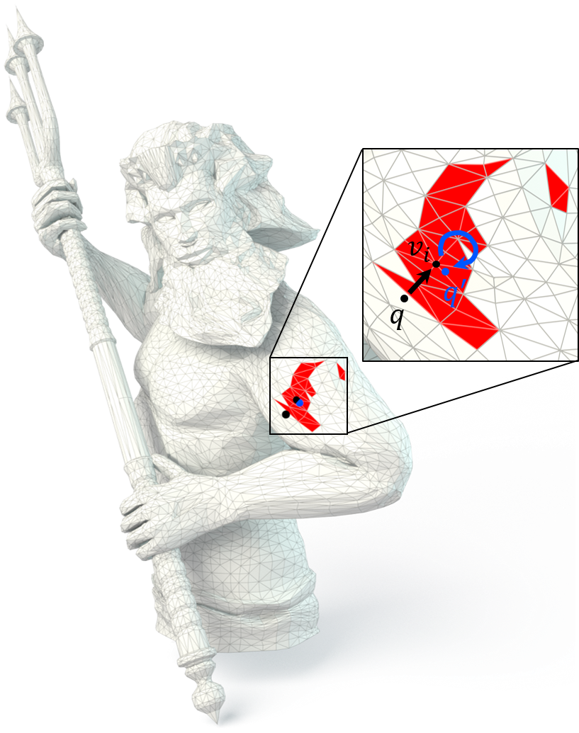
In this paper, we intend to use the KD tree (KDT), built from the vertex set , to help identify the real geometric primitive that defines the minimum distance. When users input a query point whose nearest point is found to be by KDT search, we hope that the vertex is able to keep enough clues to help find the real closest point . Suppose that the mesh edge (resp., face ) is the geometric primitive containing . We say that intercepts (resp., ). The main task of this paper is to precompute the interception table, with which the query stage proceeds by first searching the KDT and then looking up the table to report the real closest point; See Figure 1.
Let be respectively the vertex set, the edge set and the face set of a triangle mesh. Mathematically we take each vertex as a point with no dimension, each edge as an open line segment with no width, and each face as a bounded open region with no thickness. Just as the vertex set can define a Voronoi diagram in 3D, the geometric primitives in can altogether define a generalized Voronoi diagram , following the above definition. Let be ’s cell in , and be ’s cell in . We observe that intercepts (resp., ) if and only if the intersection between and (resp., ) is not empty.
Based on this observation, we give two techniques for fast interception inspection. First, we relax the intersection domain (possibly non-convex) into a convex polytope
and give an effective filtering rule for fast interception inspection. Second, we suggest a flooding procedure of interception inspection to avoid exhausting all the vertex-edge and vertex-face pairs. The couple of techniques, simple yet effective, enables one to precompute the interception table in a short period of time, e.g., about two minutes for a 1500K-face Dragon model. Note that the timing cost for accomplishing the same preprocessing task in a brute-force manner is more than one day! We conduct extensive experiments to compare our algorithm with the BVH-based point-to-mesh distance query solvers. Experimental results show that our query, with the support of the interception table, is many times faster than the SOTA methods.
2. Related Work
Two topics are related to the theme of this paper, including nearest neighbor (NN) search and BVH.
2.1. Nearest neighbor search
Given a set of points in the -dimensional space, NN search algorithms aim to find the one that is nearest to the user-specified input point . The search operation can be done efficiently by organizing the points into a tree such that large portions of the search space can be eliminated in the query stage. Most NN search algorithms include a tree construction stage and a tree-based query stage.
KDT
Suppose that we have -dimensional points , and each point of has a form of . We first find the median point to divide the other points along the first dimension. The following process can be conducted in a divide-and-conquer fashion except that the division of points is done for different dimensions alternatively. The construction is finished when all the points are arranged in the tree. In fact, each non-leaf node defines an axis-aligned hyperplane to split the space of interest into two parts.
In the query stage, the algorithm moves down the tree depending on the relative position of the query point to the splitting hyperplane. Once reaching a leaf node, the algorithm updates the best-so-far distance. Then it needs to unwind the recursion of the tree and update the current best if there is another node that gives a smaller distance. Besides the task of querying the nearest point, the KDT can also be extended in several ways, e.g., searching -nearest neighbors or retrieving points in a given hyperbox or hypersphere.
Other NN search data structures
In fact, there are many other data structures (Li et al., 2019) devised for NN search, for example, R-tree (Guttman, 1984; Beckmann et al., 1990; Kamel and Faloutsos, 1993; Berchtold et al., 1996), ball-tree (Liu et al., 2006), A-tree (Sakurai et al., 2000), BD-tree (White and Jain, 1996), SR-tree (Katayama and Satoh, 1997) and Voronoi diagrams. Although Voronoi diagrams encode the proximity between points more precisely, the construction/search of Voronoi diagram is not easy (Sharifzadeh and Shahabi, 2010; Devroye et al., 2004) especially with the increase of point dimensions. Furthermore, the operation of locating a point in a Voronoi diagram is less efficient than the KDT.
2.2. Bounding volume hierarchy
Like the KDT, a BVH (Haverkort, 2004) is a hierarchical structure to encode a set of geometric primitives. Each leaf node wraps a single geometric primitive while each non-leaf node keeps the enclosing bounding volume of a subset of geometric primitives. The BVH can be built in a top-down, bottom-up, or incremental insertion-based style, ultimately producing a tree with a bounding volume at the top. BVH has been widely used in distance query (Ytterlid and Shellshear, 2015), ray tracing (Meister et al., 2021) and collision detection (Funfzig et al., 2006; Wang and Cao, 2021).
Bounding volume types
In the past research, various types of bounding volumes have been proposed and tested.
The choice of bounding volume is a trade-off between
simplicity and tightness. On one hand, a simple bounding volume enables fast intersection tests and distance computation.
On the other hand, the bounding volume is expected to fit the enclosed geometric primitives as tight as possible. Commonly used bounding volumes include AABB (Beckmann et al., 1990; Larsson and
Akenine-Möller, 2006),
bounding sphere
(Palmer and
Grimsdale, 1995; Hubbard, 1995; Kavan and
Žára, 2005), OBB (Gottschalk
et al., 1996) and K-DOP (Klosowski et al., 1998).
More bounding structures include zonotope (Guibas
et al., 2003), pie slice (Barequet et al., 1996), ellipsoid (Liu
et al., 2007), VADOP (Coming and Staadt, 2007) and convex hull (Ehmann and Lin, 2001).
PQP
Considering that the typical discrete representation of a 3D object is a triangle mesh or a triangle soup, the task of encoding the spatial proximity is to arrange a collection of triangles into a BVH. The PQP (Larsen et al., 1999), as well as the modified version (Liu and Wang, 2010; Wang and Chen, 2013), exploits OBBs to wrap geometric primitives, facilitating fast distance query. Statistics show that PQP filters out the vast majority of triangles that do not help determine the minimum distance.
BVH acceleration techniques
Besides some works that focus on improving the quality of bounding volumes, there are some accelerated versions such as FCPW (Sawhney, 2021) and Embree (Áfra et al., 2016). For example, FCPW applies a wide BVH with vectorized traversal to accelerate its queries to geometric primitives (Sawhney, 2021). While both SIMD (Ruipu et al., 2010) and GPGPU (Tang et al., 2011) have been used to improve the performance, the required computational amount is not really reduced.
3. Insight
In this section, we provide the insight based on the 2D setting, but it is worth noting that the proposed algorithm in this paper is mainly devised for the 3D situation.
(a)(b)(c)(d)
If the given geometric objects consist of finitely many discrete 2D points , there are some tree-type structures (like the KDT) to organize them to facilitate fast query of the nearest point. In fact, the point set determines a 2D Voronoi diagram that partitions the 2D plane into cells. The task of finding the nearest point to the query point with the help of a KDT is equivalent to the task of locating in .
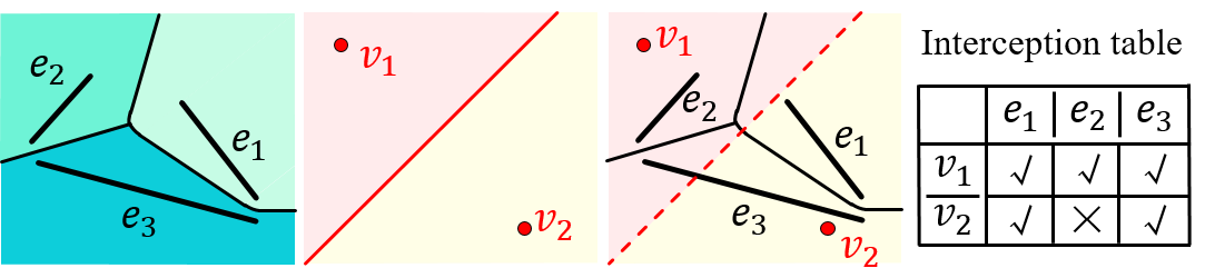
In our scenario, however, the geometric objects may be more complicated. As Figure 2(a) shows, we have three line segments . We need to report which line segment can provide the smallest distance for a query point in the 2D plane. Similarly, also induces a Voronoi diagram where different Voronoi cells are visualized in different colors. The task of querying the closest point to in , in its nature, is to locate the query point in .
The Voronoi diagram w.r.t. non-point geometric primitives has curved bisectors, which are non-trivial to compute. Furthermore, even if the generalized Voronoi diagram has been computed, it is hard for one to quickly locate the query point. This motivates us to convert the point-to-mesh distance query problem to the traditional nearest point search problem where the geometric primitives consist of finitely many points. As Figure 2(b) shows, we sample two points in the 2D plane. The Voronoi diagram is simply a straight-line bisector. Note that is not directly tied to in this example although can be chosen to be a subset of in practice.
The key idea of this paper is to speed up the process of finding the closest geometric primitive in with the help of a KDT of .
Figure 2(c) gives an overlay visualization of and . Suppose that is nearer to than . Then must be in the ’s cell of . Under this circumstance, the closest line segment to may be or or . If is nearer to than , instead, the closest line segment may be or . To summarize, is said to intercept an edge-type primitive if and only if the following search space is non-empty:
| (1) |
We can also say that is an interceptor of if the interception occurs. In this way, we obtain an interception table to keep the interception relationship between and ; See Figure 2(d).
Roughly speaking, the KDT encodes how the mesh vertices are positioned in the 3D space while the interception table encodes the principal-agent relationship between a set of points and a set of more complicated geometric primitives.
(a) (b)
4. Formulation
4.1. Problem statement
Suppose that we have a collection of triangles . Rather than simply take as a triangle soup, we assume that owns only one copy for each vertex. Let and be respectively the vertex set and the edge set. We take the vertex set as the generators to define the Voronoi diagram while taking as the generators simultaneously to define the Voronoi diagram , where each edge/face is taken as an open point set (the endpoints or the boundary excluded); See Figure 3 for illustration. Based on the observation in Section 3, the difference between and induces the interception table, i.e., a vertex intercepts an edge-type primitive if and only if the following search space is non-empty:
| (2) |
Similarly, intercepts a face-type primitive if and only if the intersection is non-empty:
| (3) |
However, and may have a curved boundary surface, making it non-trivial to determine whether the intersection domain is empty, which motivates us to study the structural features of and , and develop a fast interception inspection algorithm.
4.2. Structure of and
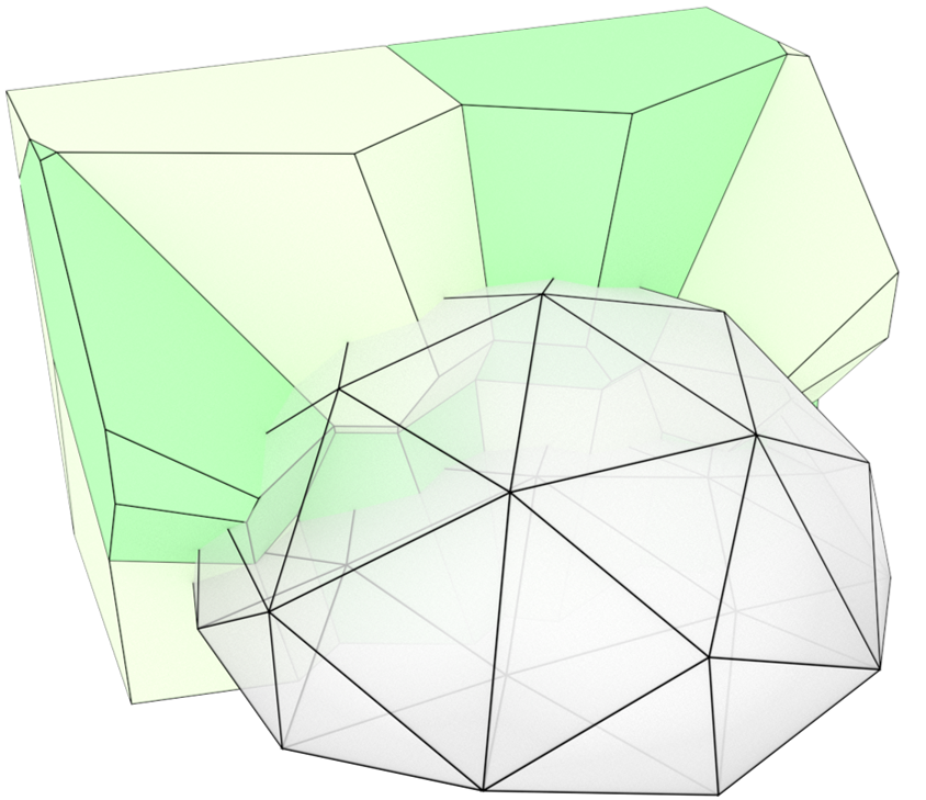
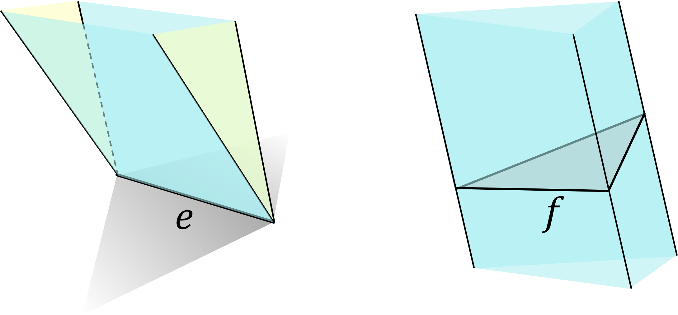
Suppose that we have a triangle face . Then contains all the points that are nearer to than to any other geometric primitive. Recall that does not include its boundary edges. If we project a point onto the plane of , then the projection must be an interior point of , satisfying . Therefore, we use the three bounding edges of to define three vertical planes, and denote the space sandwiched by the three vertical planes by , as Figure 4(b) shows. Obviously, we have
| (4) |
For an edge , can be defined similarly. As Figure 4(a) shows, the edge is adjacent to two faces, each of which defines a half space. Also, there are two half planes rooted at the endpoints of . The intersection domain by the four half spaces defines . Note that if is adjacent to more or less than two faces, can also be well defined.
Likewise, we have
| (5) |
(a)(b)
By combining and , we have the following observation.
Theorem 1.
Suppose that . Then we have
Furthermore, as the cell of encloses the vertex , the intersection between and every incident edge/face cannot be empty, which shows that must intercept the incident edges and faces.
Theorem 2.
Suppose that is a vertex. Then must intercept the edges and the faces incident to .
It’s worth noting that and are convex polyhedral domains, which can be represented by a collection of linear constraints.
4.3. Interception filtering
Suppose that , and we come to discuss in what situation intercepts . Let be the straight line of . If is an endpoint of , then must be an interceptor of .
(a)(b)
As Figure 5(a) shows, the point and the straight line determine a bisector surface that divides the whole space into two parts, where the part containing is convex. We use to denote the convex part containing while using to denote the other part. The following theorem gives a situation that cannot intercept ; See Figure 6 for 2D illustration.
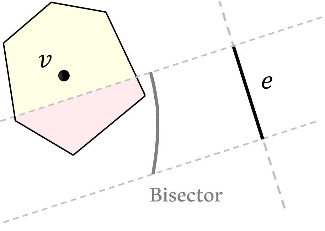
Theorem 3.
If , then cannot intercept .
Proof.
If does not intersect the vertical space of , i.e.,
then we have
due to
Otherwise, any point
must belong to , which implies that is closer to than to .
Under the assumption that intercepts , there is at least one point
such that the projection of onto is located between the two endpoints of (see Eq. (5)). Furthermore, we have and , which contradicts the fact that any point in is closer to than to . ∎
Next, we come to discuss in what situation a vertex intercepts a triangle . We suppose that the plane of is . The point and the plane determine a bisector surface, as is shown in Figure 5(b). It is easy to filter out the following interception case in a similar inference procedure.
Theorem 4.
If , then cannot intercept .
Remark. is a convex polygonal space but may be unbounded. In practical occasions, we can assume that both the vertex set and the query point are in a limited range, e.g.,
| (6) |
where is a sufficiently large constant. We can add 8 virtual points into , yielding :
| (7) |
It can be proved that the nearest point to any query point in the limited range can only be a point in , but not a virtual point. The benefit of augmenting to is that in the Voronoi diagram , the cell of each becomes bounded. Therefore, in what follows, we take , as well as or , as a bounded convex polytope.
4.4. Convexity based filtering rule
Theorem 3 points out a situation of impossible interception, i.e., if , then cannot intercept , where defines a convex and bounded polytope. Suppose that the polytope of has extreme points . Due to the convexity of and , the assertion of is equivalent to
| (8) |
Based on the fact, we propose a convexity based filtering rule as follows.
Theorem 5.
We assume that has extreme points to define the convex volume. If
| (9) |
then cannot intercept , where denotes the distance between the point and the straight line .
Theorem 6.
We assume that has extreme points to define the convex volume. If
| (10) |
then cannot intercept , where denotes the distance between the point and the plane .
Implementation
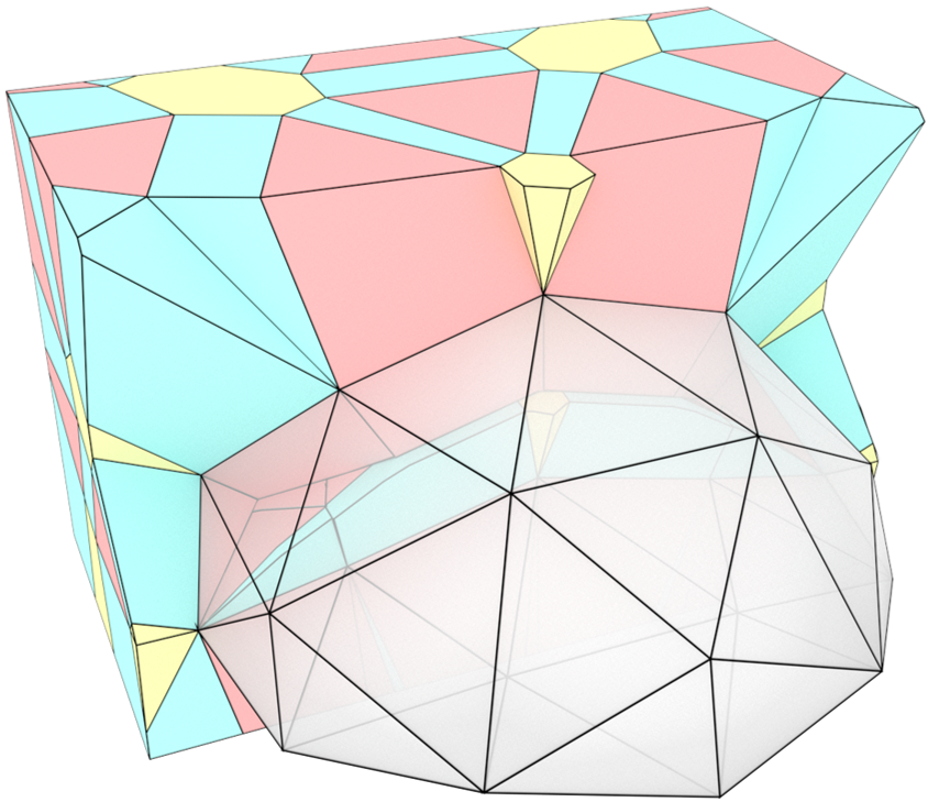
To this end, it is necessary to compute the convex polytope or to facilitate interception inspection. In fact, the operation of generating a convex polytope by plane cutting is available in CGAL (CGAL, 2022) or Geogram (Geogram, 2020), but our scenario is specific since the number of half-planes is quite limited.
Therefore, we implement plane cutting by ourselves for consideration of run-time performance.
(or ) is initialized to be ’s Voronoi cell, i.e., . During the construction of , the convex polytope is repeatedly cut by a sequence of half-planes.
![[Uncaptioned image]](/html/2308.16084/assets/fig/polytope.png)
For each corner of the convex polytope, we keep the coordinates, as well as the three half-planes that define the corner. For each edge of the convex polytope, we keep the identities of the two endpoints. As the inset figure shows, when a new half-plane comes, we remove the vertices and the edges lying on the invisible side of . If intersects a surviving edge at a new point , then defines a new corner point and replaces the invisible endpoint of at the same time.
When all the half-planes are handled, the surviving vertices are reported, facilitating the inspection of interception; See Theorem 5 and Theorem 6. Statistics show that the average time for computing (or ) is about 12 microseconds on the 20K-face Camel model, which is faster than the implementation in CGAL.
4.5. Inspection in a flooding fashion
Suppose that the Voronoi diagram of the vertex set has been precomputed. Rather than exhaustively inspect the interception between each vertex and each edge (or face), we propose to perform inspection in a flooding fashion. Initially, we build an empty interception table . For a mesh edge , we inspect the vertices in from ’s endpoints in a flooding fashion, where the neighboring relationship is defined by . Likewise, for each face , we perform flooding inspection from the three vertices of . All the detected interception pairs are kept in . We summarize the flooding algorithm for inspection of ’s interceptors in Algorithm 1. We give a theorem on verifying the correctness of the flooding inspection scheme without missing any interception.
Theorem 7.
The flooding strategy of Algorithm 1 ensures that all the interception pairs can be found.
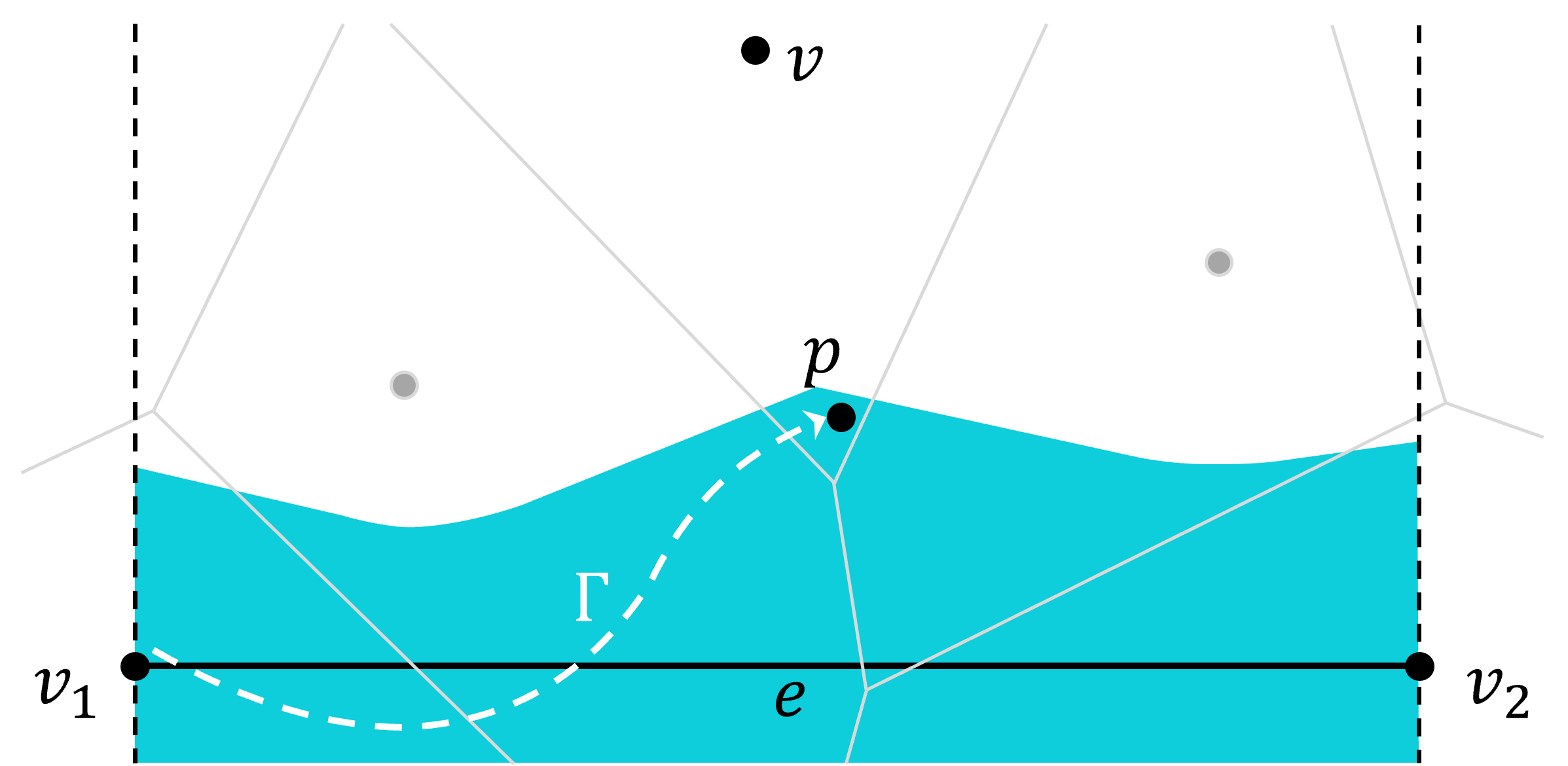
Proof.
Suppose that is an interceptor of . We come to prove that must be found in the flooding process. Our proof is based on the fact that is a connected region, which can be proved by contradiction (we ignore the proof).
As is the interceptor of , there must be at least one point, say, , such that
The connectedness of implies that there is a path between and such that is totally inside . Suppose that crosses a sequence of Voronoi cells in , denoted by . It is easy to verify the following two facts. First, is a natural interceptor of . Second, every Voronoi cell that has intersections with gives an interceptor for . Therefore, we can take as the first interceptor, and then trace the other interceptors along until is found. ∎
4.6. Further optimization in the query phase
In the query stage, we first find the nearest vertex by KDT search, followed by looking up the interception table. A naïve strategy is to enumerate all the primitives in the interception table to identify the one that is closest to the query point . However, the query becomes inefficient when the interception table is very long. Recall that an edge is said to be intercepted by if , regardless of the location of the specific query point .
Based on the discussion in Section 4.3, the assertion can be relaxed to
See Figure 8. We denote by . To this end, whether the edge contributes to the minimum distance can be reduced to check if is located in . However, is generally non-convex, making it difficult to perform the inside-outside test.
Therefore, for each edge (resp., face ) in the interception list of , we suggest enclosing (resp., ) by its bounding box and then organizing the bounding boxes into an R-tree, finally producing one R-tree per interception list.
Besides, when determining whether a primitive, say, (resp., ), can provide the minimum distance, we first check whether (resp., ) or not. Only when the assertion is true, we come to calculate the distance from to the straight line of (resp., the plane of ).
To summarize, after the nearest vertex is found by KDT search, the geometric primitives are further filtered out by R-tree. For the surviving geometric primitives, we conduct an exhaustive comparison to accomplish the point-to-mesh distance query.
5. Evaluation
We conducted experiments on a PC with AMD Ryzen 9 5950X 16-core processor. Our implementation is written in C++. We call TetGen (version 1.6.0) (Si, 2015) to compute the Voronoi diagram w.r.t. the vertex set . We first give the performance statistics of the proposed algorithm. After that, we compare our algorithm with PQP111 The modified PQP version includes a direct interface for point-to-mesh distance queries, and the code is available at https://mewangcl.github.io/Projects/MeshThickeningProj.htm. and FCPW in terms of various indicators.
Note that FCPW supports SIMD parallelism and we set the CPU based SIMD width to 4 in our experiments. There is no parallelism in PQP and our code. For each test model, we randomly sample a million query points within the 10x axis-aligned bounding box.
5.1. Interception list
Length of the interception list for a vertex
Recall that in the interception table, we keep the intercepted geometric primitives, i.e., edges and faces, for each vertex in . As different vertices have different numbers of intercepted primitives, we take the 1500K-face Dragon model as the input, shown in Figure 9, to observe how the length of the interception list of a vertex varies with the position on the surface (the horizontal axis: the length of the interception list; the vertical axis: the number of vertices). It can be seen that for most of the vertices, the length of the interception list of a vertex ranges from 20 to 100. The average length for this example is about 41. However, there is an occurrence that the interception list is very long. In Figure 9, the vertex colored with a red dot keeps 782 intercepted primitives. Once the vertex is retrieved by the KDT, it is time-consuming to exhaust every intercepted primitive in its interception list. That’s why we introduce an R-tree based filtering method (see Section 4.6) to reduce the number of candidate primitives.
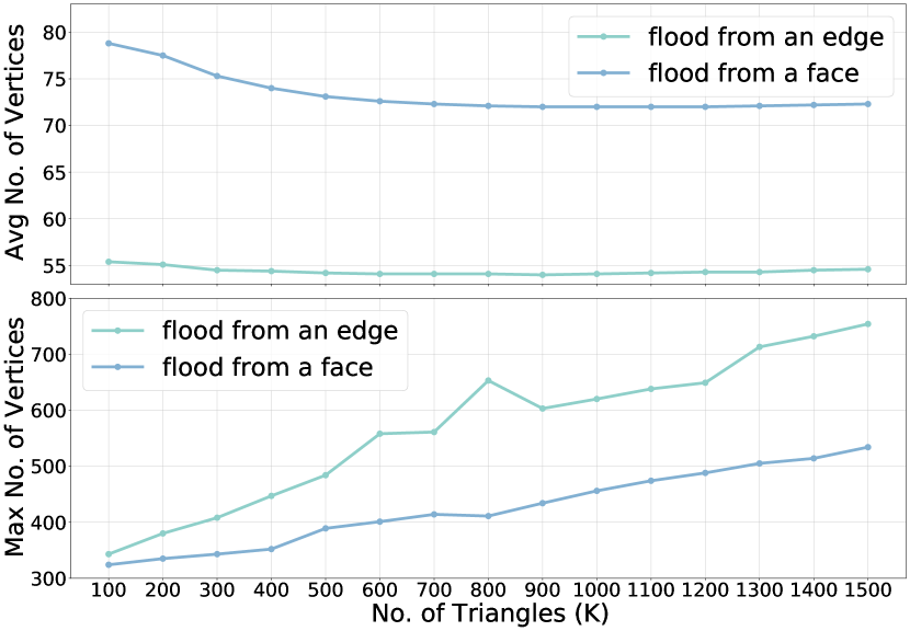
We simplify the Dragon model into 100K, 200K, , 1500K faces respectively and then record the average and maximum number of the intercepted primitives for a vertex. Statistics in Figure 10 show that the average length of interception list remains nearly unchanged with the increase of mesh resolution, but there is a slight rise in the maximum length.
| Intercepted (edges, faces) | Tested (edges, faces) | ||||||||
| Model | Faces | Avg1 | Avg2 | Max | Avg | Max | |||
| Camel | 19510 | 18.0, 26.3 | 15.0, 17.2 | 105, 130 | 5.5, 2.7 | 12, 12 | |||
| Armadillo | 99976 | 19.0, 23.6 | 17.1, 20.7 | 81, 91 | 4.7, 1.9 | 13, 13 | |||
| Sponza | 262196 | 21.4, 26.8 | 34.8, 29.4 | 296, 168 | 0.4, 0.1 | 23, 28 | |||
| Lucy | 525814 | 18.3, 23.7 | 23.1, 22.6 | 346, 232 | 4.3, 1.6 | 14, 9 | |||
| Dragon | 1499852 | 19.2, 21.7 | 16.6, 19.2 | 434, 425 | 5.1, 2.0 | 13, 13 | |||
Number of tested primitives
We must point out that different vertices have different chances of being accessed, depending on the size of the Voronoi cell . Therefore, we take the size of to weigh ’s access chance.
As Table 1 shows, the size-weighted average number (Avg2) is slightly different from the non-weighted average number (Avg1).
Recall that we propose an R-tree based filtering technique to filter out most of the primitives that do not help. It can be seen from the right side of Table 1 that both the average and maximum numbers of tested primitives, for each query, are significantly reduced. To summarize, the filtering technique is helpful in improving the overall performance, especially when there exist long interception lists. A more detailed discussion about the speed-up gain in the query performance by R-tree can be found in Section 5.3.
5.2. Preprocessing cost
Cost breakdown
The overall preprocessing cost
consists of four parts, i.e.,
1) KDT construction,
2) Voronoi diagram generation,
3) flood-based interception inspection
and 4) R-tree construction.
The cost breakdown generalizes to the 5 models ( see Table 2) as well as other tested models in large datasets.
It can be seen that the computation of the interception table takes about 90% of the total preprocessing time.
Despite this, the flooding scheme is still very helpful. If we inspect interception without flooding scheme, which requires to test every vertex-edge pair and every vertex-face pair, this brute-force manner requires more than 24 hours to accomplish the task on the 1500K-face Dragon model. The cost of interception inspection is reduced to 2 minutes with the help of the flooding scheme.
| KDT construction | Voronoi diagram | Interception inspection | R-tree construction | |||||||||
| Model | T() | Prop. | T() | Prop. | T() | Prop. | T() | Prop. | ||||
| Camel | 1.9 | 0.2% | 105.4 | 10.6% | 854.2 | 85.7% | 17.1 | 1.7% | ||||
| Armadillo | 9.4 | 0.2% | 718.8 | 15.0% | 3847.5 | 80.4% | 65.3 | 1.4% | ||||
| Sponza | 24.9 | 0.2% | 1936.2 | 12.3% | 13245.3 | 84.3% | 232.1 | 1.5% | ||||
| Lucy | 53.1 | 0.2% | 4100.0 | 16.6% | 19436.6 | 78.9% | 413.2 | 1.7% | ||||
| Dragon | 154.5 | 0.2% | 12163.0 | 12.6% | 80596.8 | 83.7% | 1093.9 | 1.1% | ||||
In Figure 11, we give the statistics about the preprocessing time on the Dragon model with varying resolutions. Although the worst-case theoretical time complexity of flooding is ( is the number of vertices and is the total number of edges and faces), the empirical time complexity is quasilinear w.r.t. . Furthermore, it can be seen from Figure 12 that the average number of examined vertices during flooding remains almost unchanged while the maximum number has a slight rise.
Comparison with existing libraries
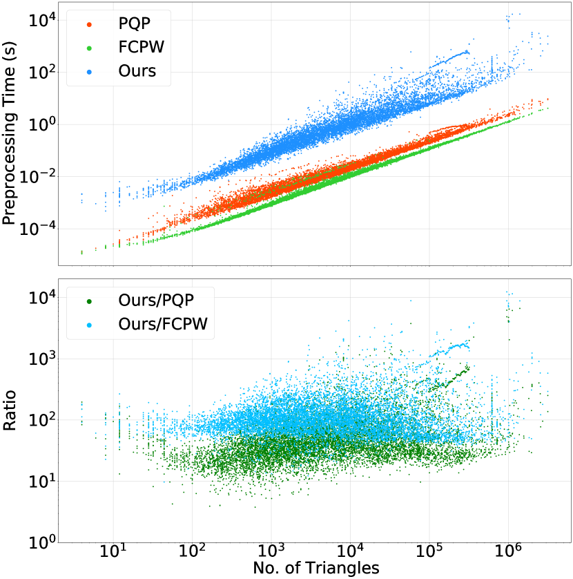
Our algorithm requires a much larger preprocessing cost than PQP and FCPW. For example, PQP and FCPW take about 4.0 seconds and 1.9 seconds respectively to construct the BVH, but our algorithm requires 137.4 seconds for preprocessing the 1500K-face Dragon model. By using the Dragon model as the test, we provide the comparison about the preprocessing cost among PQP, FCPW and ours in Figure 11. We further compare them on the Thingi10K dataset; See the statistics of the preprocessing costs in Figure 20.
5.3. Query performance
Cost breakdown
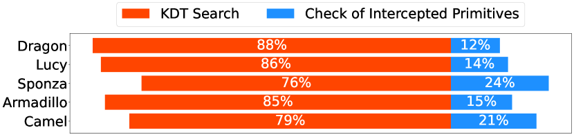
The query stage of our algorithm involves two operations: (1) finding the nearest vertex by KDT search, and (2) identifying the closest geometric primitive by visiting ’s interception list. The average timing costs of the two parts on the 1500K-face Dragon model are respectively 2.83 microseconds and 0.39 microseconds. We further plot the cost breakdown in Figure 13. It can be seen that KDT search takes over half of the total query time, which shows the effectiveness of our R-tree based filtering rule.
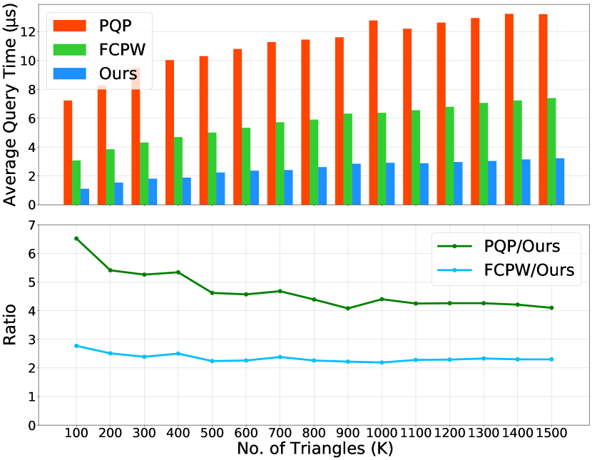
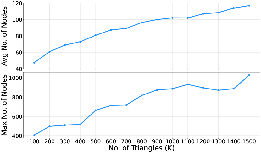
Likewise, we plot the average query cost w.r.t. mesh resolution of the Dragon model in Figure 14. It can be seen that our average query cost climbs gently with the increasing number of faces. In Figure 15, we further provide the average and maximum numbers of examined tree nodes during KDT search.
Comparison with existing libraries
Figure 14 gives a plot for visualizing the comparison about the query cost among PQP, FCPW and ours.
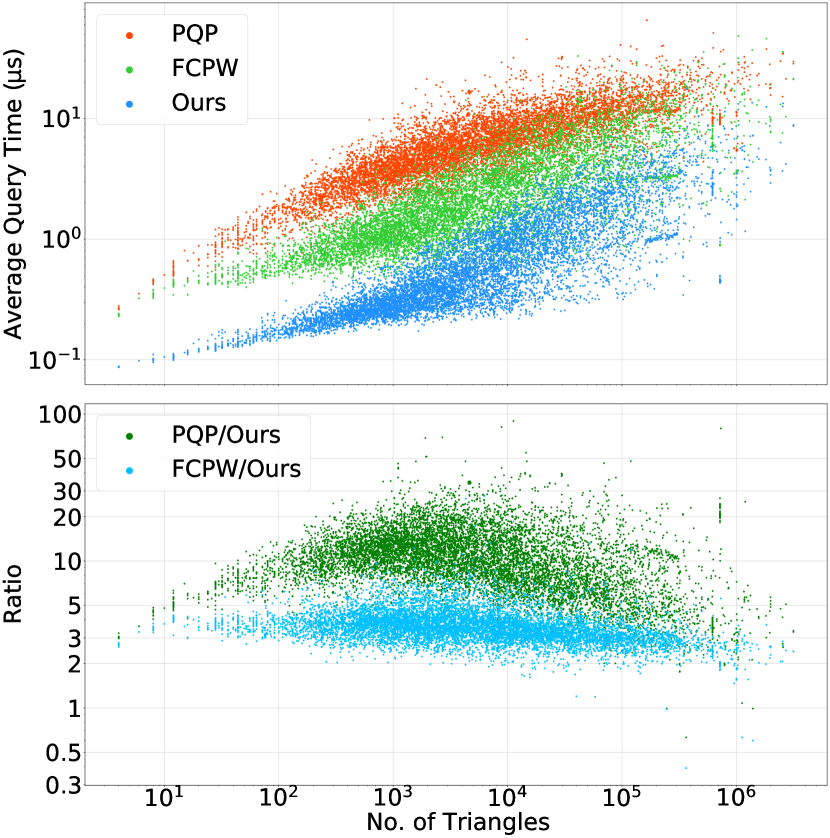
It can be seen that our algorithm runs at least 4 times as fast as PQP and 2 times faster than FCPW even on the model with 1500K faces, which shows that our algorithm has a better query performance, especially on large-sized 3D models. Figure 21 gives more comprehensive statistics about the query performance.
Near and far query points
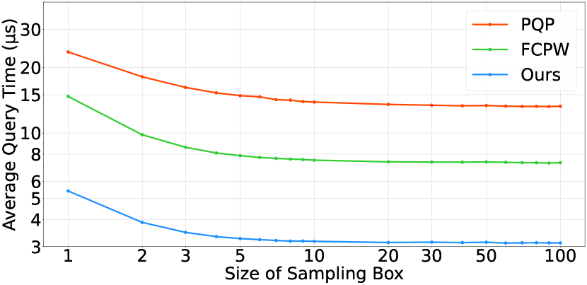
It is necessary to make clear how the query performance depends on the distance between the query point and the surface. In Figure 16, we plot the dependence of PQP’s, FCPW’s and our query performance on the distance, where the horizontal axis indicates the ratio of the maximum side length of sampling box to that of the minimum bounding box. It can be seen that, like PQP and FCPW, our query becomes more time-efficient with the increasing distance between the query point and the surface.
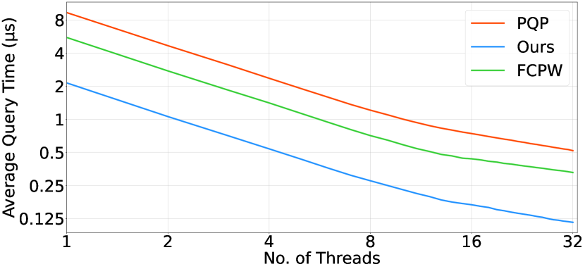
Thread-based parallelism
We perform thread-based parallelism tests, which simply divides independent queries into groups and distribute them to separate threads. As Figure 17 shows, our algorithm runs much faster than PQP and FCPW under the same thread-based parallelism and the parallel performance is close to linear.
Speed-up gain of R-tree
The use of R-tree does help when the interception list is very long. Compared with the brute-force strategy of testing all primitives in the interception list to find the closest point, the R-tree-based method can effectively filter out unnecessary primitives. Table 3 shows some examples. For general models without long interception lists, such as Camel and Armadillo, the filtering effect of R-tree is not significant.
| Tested (edges, faces) | |||||||||||||
| Model | Avg1 | Avg2 | () | () | () | () | |||||||
| Camel | 15.0, 17.2 | 5.5, 2.7 | 7.47 | 3.64 | 1.43 | 1.28 | 1.12 | ||||||
| Armadillo | 17.1, 20.7 | 4.7, 1.9 | 9.64 | 5.43 | 2.45 | 2.19 | 1.11 | ||||||
| Sponza | 34.8, 29.4 | 0.4, 0.1 | 7.69 | 0.79 | 0.57 | 0.41 | 1.36 | ||||||
| Lucy | 23.1, 22.6 | 4.3, 1.6 | 11.84 | 5.43 | 2.44 | 2.13 | 1.14 | ||||||
| Dragon | 16.6, 19.2 | 5.1, 2.0 | 13.83 | 7.56 | 3.54 | 3.34 | 1.06 | ||||||
| #378036 | 383.5, 385.7 | 6.8, 2.6 | 37.27 | 20.04 | 15.77 | 7.60 | 2.07 | ||||||
| #69078 | 356.5, 4981.7 | 5.2, 6.2 | 9.45 | 6.79 | 60.54 | 3.43 | 17.66 | ||||||
| #82324 | 743.6, 817.3 | 1.5, 0.8 | 5.18 | 1.12 | 13.43 | 0.54 | 25.06 | ||||||
| #1472696 | 2646.6 1971.6 | 0.4, 0.1 | 6.94 | 0.51 | 30.51 | 0.47 | 64.97 | ||||||
| #236143 | 2125.6, 1533.5 | 0.2, 0.1 | 5.61 | 0.79 | 37.51 | 0.37 | 100.75 | ||||||
5.4. Memory usage
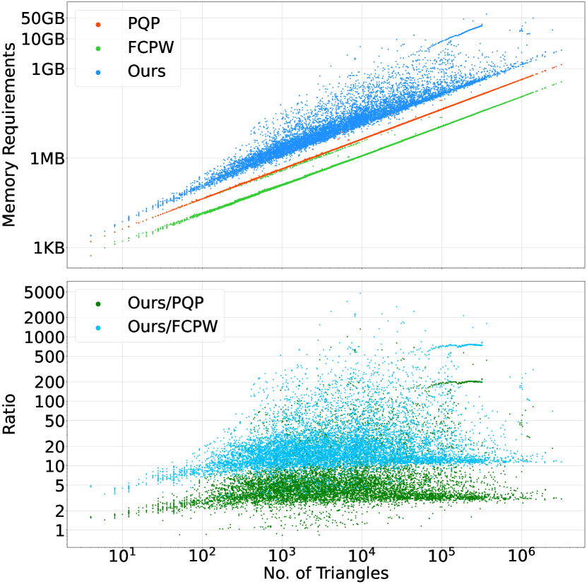
The memory requirements consist of four parts, i.e., 1) KDT structure, 2) geometric information of primitives, 3) interception lists and 4) R-tree structures. For the Dragon model, the four parts of memory usage are respectively 2%, 10%, 67% and 21%. The proportions are similar for a general input model. In contrast, our memory consumption is generally larger than PQP and FCPW. Taking the Dragon model for an example, PQP and FCPW require 0.61 GB and 0.16 GB of memory, respectively, while ours requires 1.78 GB. It is necessary to mention that FCPW uses single-precision variables while PQP and ours use double-precision variables. We give comprehensive statistics of memory consumption in Figure 22 on Thingi10K.
(a) Bad triangulation (b) Good triangulation
—c—c—c—p0.8cm¡—c—p0.8cm¡—c—p0.9cm¡—c—p0.8cm¡—c—
Model Tri Quality Bad-tri percent PQP query (s) FCPW query (s) Our query (s)
low high low high low high low high low high
![[Uncaptioned image]](/html/2308.16084/assets/fig/model_HL_1.png) 0.387 0.755 32.96% 0.13% 13.12 9.41 6.14 3.68 1.61 1.31
0.387 0.755 32.96% 0.13% 13.12 9.41 6.14 3.68 1.61 1.31
![[Uncaptioned image]](/html/2308.16084/assets/fig/model_HL_2.png) 0.344 0.603 44.47% 7.02% 15.20 6.98 4.44 3.52 1.42 1.18
0.344 0.603 44.47% 7.02% 15.20 6.98 4.44 3.52 1.42 1.18
![[Uncaptioned image]](/html/2308.16084/assets/fig/model_HL_3.png) 0.598 0.763 7.52% 0.50% 6.50 6.52 2.16 2.02 0.66 0.65
0.598 0.763 7.52% 0.50% 6.50 6.52 2.16 2.02 0.66 0.65
![[Uncaptioned image]](/html/2308.16084/assets/fig/model_HL_4.png) 0.061 0.704 87.75% 1.28% 7.53 7.21 0.76 0.83 0.31 0.31
0.061 0.704 87.75% 1.28% 7.53 7.21 0.76 0.83 0.31 0.31
![[Uncaptioned image]](/html/2308.16084/assets/fig/model_HL_5.png) 0.286 0.756 59.19% 3.29% 15.98 8.66 3.68 5.22 1.05 1.95
0.286 0.756 59.19% 3.29% 15.98 8.66 3.68 5.22 1.05 1.95
![[Uncaptioned image]](/html/2308.16084/assets/fig/model_HL_6.png) 0.292 0.621 58.39% 3.17% 24.96 15.02 11.24 5.54 2.72 1.66
0.292 0.621 58.39% 3.17% 24.96 15.02 11.24 5.54 2.72 1.66
5.5. Extreme tests
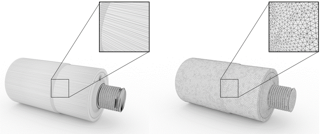
Poor triangulation quality
Generally speaking, irregularly shaped triangle faces would cause difficulties in the node splitting procedure of BVH structure generation and affect the performance of closest point query. It is necessary to observe if poor triangulation slows down the query performance of our algorithm. We select six poorly-triangulated models from the Thingi10K dataset and for each of them, we use the mesh optimization tool (Hoppe et al., 1993) to get a high-quality counterpart with the same number of triangles. The quality of a triangle can be measured by
where are respectively the area, the half-perimeter of triangle and the longest edge length. ranges from 0 to 1, and equals 1 when is a regular triangle. Table 5.4 gives the overall triangle quality as well as the ratio of bad triangles. Here a triangle is considered to “bad” if the minimum angle is less than 10 degrees. Statistics show that our query performance does not have a conspicuous drop when the triangulation quality is diminished. Taking the Water-Bottle model (as shown in Figure 18) for an example, our average query cost is 1.95s on the high-quality model while the query cost becomes 1.05s on the poorly-triangulated model. In contrast, PQP is sensitive to triangle quality, and the query cost increases from 8.66s to 15.98s when the triangulation quality is diminished. It shows that our query algorithm is less sensitive to triangle quality than BVH.
(a) (b) (c)
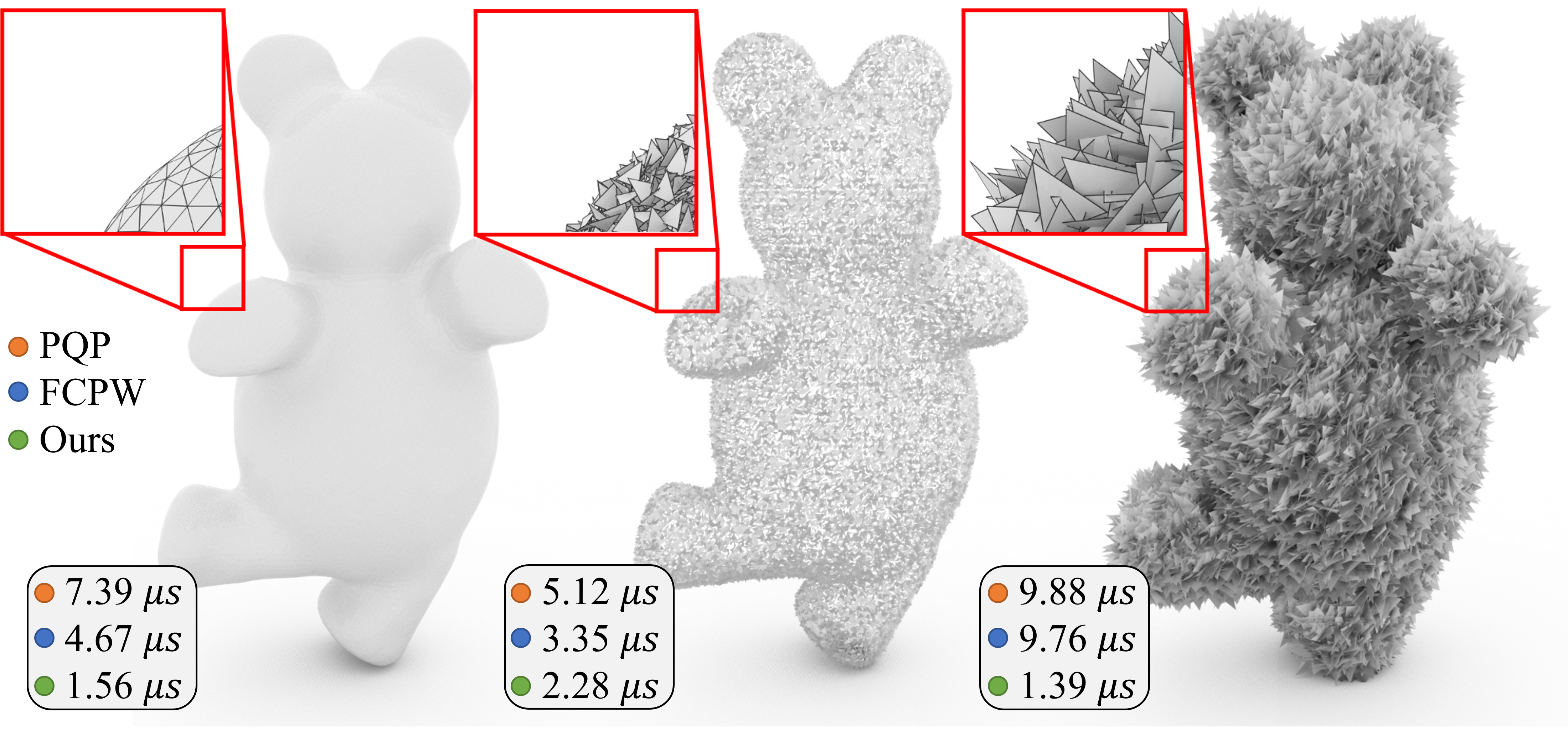
Triangle soup
Figure 19 shows three versions of the 20K-face Bear model, i.e., watertight triangle mesh, gapped triangles and a triangle soup with high penetration. The statistics of query speed are available in Figure 19. For the watertight Bear model, our query algorithm runs about 5 times as fast as PQP, and 3 times as fast as FCPW. Figure 19(b) and Figure 19(c) show that the comparative advantage over them becomes smaller for gapped triangles whereas becomes larger in the presence of high penetration.
Mixed primitives
We make tests on a mixed set of segments and triangles.
By combining the triangular mesh of Armadillo model and the wireframe of Camel model, we synthesize a mixed set of geometric primitives. Experimental results show that our algorithm is 3.8 times as fast as FCPW (PQP does not support this kind of input).
5.6. Tests on Thingi10K
Thingi10K (Zhou and Jacobson, 2016) is a large scale 3D dataset that contains diverse models.
In order to make a comprehensive comparison among PQP, FCPW and our algorithm, we run them on the full Thingi10K dataset to compare the preprocessing cost (see Figure 20), the query cost (see Figure 21) and the memory requirements (see Figure 22). Based on the statistics, we observe that our algorithm achieves a higher query performance at the cost of preprocessing and memory usage. Generally speaking, our algorithm runs 2 to 10 times faster than PQP and FCPW.
6. Conclusion and Limitations
In this paper, we develop a novel algorithmic paradigm, named P2M, to solve the problem of point-to-mesh distance query. P2M needs to precompute a pair of data structures including a KDT of mesh vertices and an interception table that encodes the principal-agent relationship between vertices and edges/faces, such that the query stage proceeds by first searching the KDT and then looking up the interception table to retrieve the closest geometric primitive. We give rigorous proofs about the correctness and propose a set of strategies for speeding up the preprocessing stage and the query stage. We conduct extensive experiments to evaluate our approach. Experimental results show that our algorithm runs many times faster than the SOTAs.
However, in its current state, our algorithm still needs comprehensive improvement. First, the construction of the interception table is still time-consuming. Statistics show that in the time-consuming interception inspection phase, about 85% of visited vertices are checked but found not to be an interceptor during flooding. One potential research direction is to quickly exclude the non-interceptor vertices by some filtering techniques. Second, the interception table becomes very long for a highly symmetrical shape. For example, if the input is a spherical surface, then each vertex intercepts any triangle. Last but not least, PQP supports closest point query, line-surface intersection and collision detection at the same time, but our algorithm only supports closest point query. In the future, we shall further improve the algorithm in terms of the above-mentioned aspects.
7. Acknowledgements
The authors would like to thank the anonymous reviewers for their valuable comments and suggestions. This work is supported by National Key R&D Program of China (2021YFB1715900), National Natural Science Foundation of China (62002190, 62272277, 62072284), and Natural Science Foundation of Shandong Province (ZR2020MF036). Besides, the authors would like to express their gratitude to Professor Charlie C.L. Wang for providing a modified version of PQP that supports point-to-mesh distance queries.
References
- (1)
- Abbasifard et al. (2014) Mohammad Reza Abbasifard, Bijan Ghahremani, and Hassan Naderi. 2014. A survey on nearest neighbor search methods. International Journal of Computer Applications 95, 25 (2014).
- Áfra et al. (2016) Attila T Áfra, Ingo Wald, Carsten Benthin, and Sven Woop. 2016. Embree ray tracing kernels: overview and new features. ACM SIGGRAPH 2016 Talks (2016), 1–2.
- Auer and Westermann (2013) Stefan Auer and Rüdiger Westermann. 2013. A semi-Lagrangian closest point method for deforming surfaces. In Computer Graphics Forum, Vol. 32. Wiley Online Library, 207–214.
- Barequet et al. (1996) Gill Barequet, Bernard Chazelle, Leonidas J Guibas, Joseph SB Mitchell, and Ayellet Tal. 1996. BOXTREE: A hierarchical representation for surfaces in 3D. In Computer Graphics Forum, Vol. 15. Wiley Online Library, 387–396.
- Beckmann et al. (1990) Norbert Beckmann, Hans-Peter Kriegel, Ralf Schneider, and Bernhard Seeger. 1990. The R*-tree: An efficient and robust access method for points and rectangles. In Proceedings of the 1990 ACM SIGMOD international conference on Management of data. 322–331.
- Berchtold et al. (1996) Stefan Berchtold, Daniel A Keim, and Hans-Peter Kriegel. 1996. The X-tree: An index structure for high-dimensional data. In Very Large Data-Bases. 28–39.
- CGAL (2022) CGAL. 2022. The Computational Geometry Algorithms Library. https://www.cgal.org/.
- Coming and Staadt (2007) Daniel S Coming and Oliver G Staadt. 2007. Velocity-aligned discrete oriented polytopes for dynamic collision detection. IEEE Transactions on Visualization and Computer Graphics 14, 1 (2007), 1–12.
- Devroye et al. (2004) Luc Devroye, Christophe Lemaire, and Jean-Michel Moreau. 2004. Expected time analysis for Delaunay point location. Computational Geometry 29, 2 (2004), 61–89. https://doi.org/10.1016/j.comgeo.2004.02.002
- Ehmann and Lin (2001) Stephen A Ehmann and Ming C Lin. 2001. Accurate and fast proximity queries between polyhedra using convex surface decomposition. In Computer Graphics Forum, Vol. 20. Wiley Online Library, 500–511.
- Funfzig et al. (2006) Christoph Funfzig, Torsten Ullrich, and Dieter W Fellner. 2006. Hierarchical spherical distance fields for collision detection. IEEE Computer Graphics and Applications 26, 1 (2006), 64–74.
- Geogram (2020) Geogram. 2020. A programming library of geometric algorithms. http://alice.loria.fr/software/geogram/doc/html/index.html.
- Gottschalk et al. (1996) Stefan Gottschalk, Ming C Lin, and Dinesh Manocha. 1996. OBBTree: A hierarchical structure for rapid interference detection. In Proceedings of the 23rd annual conference on Computer graphics and interactive techniques. 171–180.
- Guezlec (2001) Andre Guezlec. 2001. ” Meshsweeper”: dynamic point-to-polygonal mesh distance and applications. IEEE Transactions on Visualization and Computer Graphics 7, 1 (2001), 47–61.
- Guibas et al. (2003) Leonidas J Guibas, An Thanh Nguyen, and Li Zhang. 2003. Zonotopes as bounding volumes. In SODA, Vol. 3. 803–812.
- Guttman (1984) Antonin Guttman. 1984. R-trees: A dynamic index structure for spatial searching. In Proceedings of the 1984 ACM SIGMOD international conference on Management of data. 47–57.
- Haverkort (2004) Herman J Haverkort. 2004. Introduction to bounding volume hierarchies. Part of the PhD thesis, Utrecht University (2004).
- Hoppe et al. (1993) Hugues Hoppe, Tony DeRose, Tom Duchamp, John McDonald, and Werner Stuetzle. 1993. Mesh optimization. In Proceedings of the 20th annual conference on Computer graphics and interactive techniques. 19–26.
- Hubbard (1995) Philip Martyn Hubbard. 1995. Collision detection for interactive graphics applications. IEEE Transactions on Visualization and Computer Graphics 1, 3 (1995), 218–230.
- Kamel and Faloutsos (1993) Ibrahim Kamel and Christos Faloutsos. 1993. Hilbert R-tree: An improved R-tree using fractals. Technical Report.
- Katayama and Satoh (1997) Norio Katayama and Shin’ichi Satoh. 1997. The SR-tree: An index structure for high-dimensional nearest neighbor queries. ACM Sigmod Record 26, 2 (1997), 369–380.
- Kavan and Žára (2005) Ladislav Kavan and Jiří Žára. 2005. Fast collision detection for skeletally deformable models. In Computer Graphics Forum, Vol. 24. Blackwell Publishing, Inc Oxford, UK and Boston, USA, 363–372.
- Klosowski et al. (1998) James T Klosowski, Martin Held, Joseph SB Mitchell, Henry Sowizral, and Karel Zikan. 1998. Efficient collision detection using bounding volume hierarchies of k-DOPs. IEEE Transactions on Visualization and Computer Graphics 4, 1 (1998), 21–36.
- Larsen et al. (1999) E. Scott Larsen, Stefan Gottschalk, Ming C. Lin, and Dinesh Manocha. 1999. Fast Proximity Queries with Swept Sphere Volumes.
- Larsson and Akenine-Möller (2006) Thomas Larsson and Tomas Akenine-Möller. 2006. A dynamic bounding volume hierarchy for generalized collision detection. Computers & Graphics 30, 3 (2006), 450–459.
- Li et al. (2019) Wen Li, Ying Zhang, Yifang Sun, Wei Wang, Mingjie Li, Wenjie Zhang, and Xuemin Lin. 2019. Approximate nearest neighbor search on high dimensional data—experiments, analyses, and improvement. IEEE Transactions on Knowledge and Data Engineering 32, 8 (2019), 1475–1488.
- Liu and Wang (2010) Shengjun Liu and Charlie CL Wang. 2010. Fast intersection-free offset surface generation from freeform models with triangular meshes. IEEE Transactions on Automation Science and Engineering 8, 2 (2010), 347–360.
- Liu et al. (2007) Shengjun Liu, Charlie CL Wang, Kin-Chuen Hui, Xiaogang Jin, and Hanli Zhao. 2007. Ellipsoid-tree construction for solid objects. In Proceedings of the 2007 ACM symposium on Solid and physical modeling. 303–308.
- Liu et al. (2006) Ting Liu, Andrew W Moore, Alexander Gray, and Claire Cardie. 2006. New Algorithms for Efficient High-Dimensional Nonparametric Classification. Journal of Machine Learning Research 7, 6 (2006).
- Meister et al. (2021) Daniel Meister, Shinji Ogaki, Carsten Benthin, Michael J Doyle, Michael Guthe, and Jiří Bittner. 2021. A Survey on Bounding Volume Hierarchies for Ray Tracing. In Computer Graphics Forum, Vol. 40. Wiley Online Library, 683–712.
- Palmer and Grimsdale (1995) Ian J. Palmer and Richard L. Grimsdale. 1995. Collision detection for animation using sphere-trees. In Computer Graphics Forum, Vol. 14. Wiley Online Library, 105–116.
- Ruipu et al. (2010) Tan Ruipu, Zhao Wei, and Li Jing. 2010. The Study of Parallel Collision Detection Algorithms. In 2010 International Conference on Multimedia Technology. IEEE, 1–4.
- Sakurai et al. (2000) Yasushi Sakurai, Masatoshi Yoshikawa, Shunsuke Uemura, Haruhiko Kojima, et al. 2000. The A-tree: An index structure for high-dimensional spaces using relative approximation. In VLDB, Vol. 2000. Citeseer, 5–16.
- Sawhney (2021) Rohan Sawhney. 2021. FCPW: Fastest Closest Points in the West. https://github.com/rohan-sawhney/fcpw.
- Sharifzadeh and Shahabi (2010) Mehdi Sharifzadeh and Cyrus Shahabi. 2010. VoR-Tree: R-Trees with Voronoi Diagrams for Efficient Processing of Spatial Nearest Neighbor Queries. Proc. VLDB Endow. 3, 1–2 (sep 2010), 1231–1242. https://doi.org/10.14778/1920841.1920994
- Si (2015) Hang Si. 2015. TetGen, a Delaunay-Based Quality Tetrahedral Mesh Generator. ACM Transactions on Mathematical Software (TOMS) 41 (2015), 1 – 36.
- Tang et al. (2011) Min Tang, Dinesh Manocha, Jiang Lin, and Ruofeng Tong. 2011. Collision-streams: Fast GPU-based collision detection for deformable models. In Symposium on interactive 3D graphics and games. 63–70.
- Wald et al. (2019) Ingo Wald, Will Usher, Nathan Morrical, Laura Lediaev, and Valerio Pascucci. 2019. RTX Beyond Ray Tracing: Exploring the Use of Hardware Ray Tracing Cores for Tet-Mesh Point Location.. In High Performance Graphics (Short Papers). 7–13.
- Wang and Chen (2013) Charlie CL Wang and Yong Chen. 2013. Thickening freeform surfaces for solid fabrication. Rapid Prototyping Journal 19, 6 (2013), 395–406.
- Wang and Cao (2021) Monan Wang and Jiaqi Cao. 2021. A review of collision detection for deformable objects. Computer Animation and Virtual Worlds (2021), e1987.
- White and Jain (1996) David A White and Ramesh Jain. 1996. Similarity indexing with the SS-tree. In Proceedings of the Twelfth International Conference on Data Engineering. IEEE, 516–523.
- Ytterlid and Shellshear (2015) Robin Ytterlid and Evan Shellshear. 2015. BVH split strategies for fast distance queries. Journal of Computer Graphics Techniques (JCGT) 4, 1 (2015), 1–25.
- Zhou and Jacobson (2016) Qingnan Zhou and Alec Jacobson. 2016. Thingi10K: A Dataset of 10,000 3D-Printing Models. https://doi.org/10.48550/ARXIV.1605.04797