Giant piezoelectricity driven by Thouless pump in conjugated polymers

Abstract

Piezoelectricity of organic polymers has attracted increasing interest because of several advantages they exhibit over traditional inorganic ceramics. While most organic piezoelectrics rely on the presence of intrinsic local dipoles, a highly nonlocal electronic polarization can be foreseen in conjugated polymers, characterised by delocalized and highly responsive $\pi$-electrons. These 1D systems represent a physical realization of a Thouless pump, a mechanism of adiabatic charge transport of topological nature which results, as shown in this work, in anomalously large dynamical effective charges, inversely proportional to the band gap energy. A structural (ferroelectric) phase transition further contributes to an enhancement of the piezoelectric response reminiscent of that observed in piezoelectric perovskites close to morphotropic phase boundaries. First-principles Density Functional Theory (DFT) calculations performed in two representative conjugated polymers using hybrid functionals, show that state-of-the-art organic piezoelectric are outperformed by piezoelectric conjugated polymers, mostly thanks to strongly anomalous effective charges of carbon, larger than 5$e$ – ordinary values being of the order of 1$e$ – and reaching the giant value of 30$e$ for band gaps of the order of 1 eV.

Introduction

Piezoelectricity is a well known phenomenon characterising those materials which have the property to generate a surface charge, and hence an electric tension, when subject to a stress, or conversely to deform elastically in response to an external electric field. Thanks to the possibility they offer to convert mechanical energy into electrical energy and vice-versa, piezoelectric materials are of great interest in various fields and for many applications, from macro- to microscopic electromechanical devices, to energy harvesting and much more[1, 2]. The most widely used piezoelectric materials are inorganic perovskites, such as lead zirconate titanate (PZT), for their high electromechanical response[3, 4, 5]. However, inorganic materials have very low mechanical flexibility, high fabrication costs and often are toxic because of the lead they contain. These facts motivated an intense research activity aimed at developing and identifying lead-free piezoelectric ceramics[5, 6]. A promising alternative is to exploit piezoelectric properties of organic materials, a route that has been trodden with some success since early 1990s, mostly focusing on the wide class of organic polymers displaying high flexibility, low fabrication costs and bio-compatibility[7, 8, 9, 10]. In this context, the most studied organic piezoelectric is polyvinylidene fluoride (PVDF)[8, 11], a saturated polymer derived from polyethylene and comprising molecular units with net (electrical) dipole moments, thus giving rise to ferroelectricity of conformational origin due to the rotation of chains’ segments from non-polar to polar isomers.

Despite the intense research efforts and the progress made in the field of organic piezoelectrics, to date inorganic ceramics still display much better piezoelectric performance than organic counterparts. The piezoelectric response in PZT and related inorganic materials is strongly enhanced at morphotropic phase boundaries (MPB), marking a composition-driven structural transition between two competing, nearly energetically degenerate phases with distinct symmetries[12, 13, 14]. On general grounds, the properties enhancement close to such phase transition may be traced back to the flattening of free-energy surfaces, easing polarization extension and/or rotation, as extensively discussed and observed mostly in perovskite oxides[15]. Recently, the concept of MPB has been loosely extended to the family of P(VDF-TrFE) copolymers[16, 17]. Here, the introduction of different TrFE monomers in the semicrystalline PVDF structure has been proposed to lead to an enhanced conformational competition reminiscent of the structural competition realized at MPB, further suggesting an optimal chemical composition for maximizing the piezoelectric coefficient. Even though at the optimal ”morphotropic” composition the piezoelectric coefficient roughly doubles the typical values of PVDF, it is still smaller by one order of magnitude compared to characteristic piezoelectric coefficients of inorganic oxide ceramics such as PZT.

Beside saturated polymers as PVDF and P(VDF-TrFE), whose ferroelectric and piezoelectric properties rely on the ordering of built-in molecular dipoles and as such require appropriate poling treatments, a natural alternative choice is represented by conjugated polymers, such as archetypical polyacetylene (PA). Characterised by a delocalised $\pi-$orbital along their backbone, these polymers are widely studied for their peculiar electronic properties[18, 19]. If specific symmetry-lowering effects allowing for piezoelectricity and ferroelectricity are met in a conjugated polymer, one may expect a large polar response of electronic origin due to the redistribution of the responsive $\pi-$electronic density along the polymer’s backbone. Because of the delocalized nature of conjugated $\pi-$state (of Bloch-type in an infinite periodic chain), small changes of atomic positions may lead to a global shift of electrons, revealing the strong nonlocal and ultimately topological character of electronic polarization in these quasi-1D systems[20]. Indeed, conjugated polymers have been theoretically put forward as a potential new class of “electronic ferroelectrics”[21].

In order to explore the potential piezoelectricity of conjugated polymers, we adopt the simple model originally introduced by Rice and Mele to study soliton excitations of linearly conjugated diatomic polymers[22], later become a prototypical model for 1D ferroelectricity[20, 23] and Thouless adiabatic pumping[24]. We find that polar responses, such as Born effective charges and piezoelectric coefficients, can be strongly enhanced close to the dimerization phase transition characterized by a bond-length alternation (BLA) between neighboring atoms along the chain. This transition can be controlled by changes in the chemical composition of the polymers or by tuning the electron-phonon (e-ph) interaction, that is expected to be sensitive to the dielectric environment of individual chains. The strength of the piezoelectric effect is found to be determined partly by the MPB-like enhancement – relying on the second-order nature of the transition –, but mostly by a giant effective charge, ultimately due to the topological nature of Thouless’ adiabatic charge transport in this class of materials. We verified the model-based predictions and theoretical picture by performing Density Functional Theory (DFT) calculations using a range-separated hybrid functional on two prototypical conjugated polymers derived from polyacetylene, confirming strong enhancement of effective charge and consequently of piezoelectric response, that is found to be larger than the one observed in the celebrated organic piezoelectric PVDF for a wide range of parameters.

Results

A model for piezoelectric conjugated polymers

To study the effects of strain on conjugated polymers, we generalise the Rice-Mele model[22] of a 1D linear chain with a unit cell of length $a_{0}$ containing two atoms. The only possible strains for a 1D infinite periodic chain are contraction/dilatation of the unit cell, defined by $a(\epsilon)=a_{0}(1+\epsilon)$, where the adimensional parameter $\epsilon$ quantifies the strain along the direction of the chain. In a nearest neighbours tight-binding approximation, the modulation of the hopping energy between atoms at site $i$ and $i+1$ can be modelled at linear order in atoms’ displacement and strain as $t_{i,i+1}=t(\epsilon)+(-1)^{i+1}\delta t(\epsilon)$, with

$$t(\epsilon) =t_{0}(1-\beta\epsilon),$$ (1)

$$\delta t(\epsilon) =-t_{0}\beta(1+\epsilon)u(\epsilon).$$ (2)

Equation (1) accounts for the effect of strain on the hopping energy $t_{0}$ between equidistant atoms, while Equation (2) describes the variation with respect to $t(\epsilon)$ caused by atoms’ displacement; at the lowest order, we can assume the same adimensional e-ph coupling parameter $\beta>0$ in describing both effects. The term $u(\epsilon)$ is an adimensional fractional coordinate measuring the relative displacement of the two atoms in the unit cell, as defined in the Methods. We indicate with the term $\Delta\geq 0$ the on-site energy difference between neighbours. If $\Delta=0$, the atoms in the unit cell are equivalent and we recover the well-known SSH model[25], used to describe polyacetylene. However, in order to have a non-trivial polar response, it is necessary to break atoms’ equivalence ($\Delta\neq 0$) as, e.g., in substituted polyacetylenes (SPA)[26], a class of conjugated polymers formed by inequivalent monomers which can be obtained substituting (one of) the atoms in the C₂H₂ unit of PA with some element(s) or compound(s). A representation of the model is in the insets of Figure 1a). For simplicity, we consider only longitudinal displacements, parallel to the linear-chain direction. As we are interested in the equilibrium structures at $T=0~{}K$, we define the optimal displacement $\overline{u}$ as the one which minimises the total energy, given a set of material-dependent parameters and a strain. For more information on the model and the derivation of the above quantities, see the Methods and the Supplementary Information.

In the absence of strain ($\epsilon=0$), the properties of the model are well known. In the SSH model ($\Delta=0$) a finite $\overline{u}\neq 0$ is allowed by an infinitely small e-ph interaction, conjuring with a Fermi-surface nesting and Peierls electronic instability to produce a dimerized phase with bond-length alternation and the opening of a gap in the energy spectrum $E_{\mathrm{gap}}=4|\delta t|=4\beta t_{0}\overline{u}$. Breaking the equivalence between atoms ($\Delta\neq 0$) also opens a gap which is expected to counteract the Peierls instability and the related bond dimerization. The lower-symmetry structure can be stabilised only by a finite and strong enough e-ph interaction, resulting in a gap $E_{\mathrm{gap}}=2\sqrt{\Delta^{2}+4\delta t^{2}}=2\sqrt{\Delta^{2}+4(\beta t_{0}\overline{u})^{2}}$. Indeed, as shown in Figure 1a), increasing $\Delta$ at fixed e-ph coupling up to a critical value $\Delta_{\mathrm{c}}$ induces a second order structural phase transition with order parameter $\overline{u}$ between a distorted ($\overline{u}\neq 0$) and a higher-symmetric undimerized ($\overline{u}=0$) phase, both displaying an insulating character with a finite band-gap (see Supplementary Information). In a 2D parametric ($\Delta,\delta t$)-space the origin of the axes corresponds to a metallic system while the rest of the space to an insulator. It is known that if the system undergoes an adiabatic evolution along a loop enclosing the origin of this space, a quantised charge $|e|$ is pumped out. This is a prototypical example of the adiabatic charge transport known as Thouless’ pump[27, 24] realised for example in ultracold fermions[28]. The crucial ingredient is the presence of the metallic point in the domain enclosed by the loop and, in this sense, it is an example of topological phenomenon (see Supplementary Information). Previous studies on low-dimensional systems showed how topology may reflect onto polar responses, resulting, e.g., in electronic polarization in quasi-1D systems[20] or in large effective charges and piezoelectric coefficients directly related to valley Chern numbers in 2D systems[29, 30].

Morphotropic-like enhancement of the piezoelectric response

In order to have a non-trivial piezoelectric response, the chain must not have points of inversion symmetry, a requirement that is met when the equivalence between atoms is broken in a distorted chain, i.e. both $\Delta\neq 0$ and $\overline{u}\neq 0$. In this case, the chain becomes also ferroelectric with a net dipole moment per unit cell $P$[23]. The electromechanical response is quantified by the piezoelectric coefficient $c_{\mathrm{piezo}}$, defined as the variation of $P$ due to an applied homogeneous strain $\epsilon$, namely

$$c_{\mathrm{piezo}}=\left.\frac{\mathrm{d}P(\epsilon,\overline{u}(\epsilon))}{\mathrm{d}\epsilon}\right|_{\epsilon=0}=c_{\mathrm{piezo}}^{\mathrm{c.i.}}+c_{\mathrm{piezo}}^{\mathrm{i.r.}}$$ (3)

where the derivative of $P$ is decomposed in two contributions. The first one is the so-called clamped ions term

$$c_{\mathrm{piezo}}^{\mathrm{c.i.}}=\left.\frac{\partial P(\epsilon,\overline{u}(\epsilon))}{\partial\epsilon}\right|_{\epsilon=0}$$ (4)

which is obtained keeping fixed the relative position of the ions in the unit cell, i.e., for fixed internal fractional coordinate $\overline{u}_{0}=\overline{u}(0)$. It can be shown (see Methods) that $|c_{\mathrm{piezo}}^{\mathrm{c.i.}}|\leq|e|\beta/2\pi$. The second term of Equation (3) takes into account the effect of strain on the internal coordinate $\overline{u}(\epsilon)$ and defines the internal relaxation contribution

$$c_{\mathrm{piezo}}^{\mathrm{i.r.}}=Z^{*}(\overline{u}_{0})\left.\frac{\partial\overline{u}(\epsilon)}{\partial\epsilon}\right|_{\epsilon=0}$$ (5)

where we defined the effective charge $Z^{*}$, namely a measure of how rigidly the electronic charge distribution follows the displacement of the nuclei, as

$$Z^{*}=\frac{\partial P}{\partial u}.$$ (6)

The inclusion of strain in the Rice-Mele model affects explicitly the critical value $\Delta_{\mathrm{c}}(\epsilon)$ of the phase transition. The behaviour of $\overline{u}(\epsilon)$ as $\Delta$ approaches $\Delta_{\mathrm{c}}(\epsilon)$ is shown in Figure 1a), following the expected behaviour $\overline{u}(\epsilon)\propto|\Delta-\Delta_{\mathrm{c}}(\epsilon)|^{1/2}$ of the order parameter of second-order phase transitions (see Supplementary Information). It thus follows that:

$$\left.\frac{\partial\overline{u}(\epsilon)}{\partial\epsilon}\right|_{\epsilon=0}\propto\frac{1}{|\Delta-\Delta_{\mathrm{c}}(0)|^{1/2}}.$$ (7)

Equation (7) implies that the internal relaxation term diverges as we approach the critical point $\Delta_{\mathrm{c}}(\epsilon)$ from the distorted phase, in analogy with the MPB mechanism at play in some ferroelectric oxides. Indeed, as the $\Delta$ parameter of the Rice-Mele model accounts for the composition of the system, it allows to continuously tune a morphotropic-like phase transition from the distorted phase (lower symmetry, ferroelectric) to the undistorted one (higher symmetry, paraelectric). Furthermore, we highlight that, at a fixed $\Delta\neq 0$ suppressing the Peierls electronic instability, the second-order phase transition can be driven by the e-ph coupling, allowing one to define a critical value $\beta_{c}$ separating the undimerized and dimerized phases (see Supplementary Information). Clearly, the order parameter as a function of the variable driving the transition would still follow the expected behaviour $\overline{u}(\epsilon)\propto|\beta-\beta_{c}(\epsilon)|^{1/2}$, implying:

$$\left.\frac{\partial\overline{u}(\epsilon)}{\partial\epsilon}\right|_{\epsilon=0}\propto\frac{1}{|\beta-\beta_{c}(0)|^{1/2}}.$$ (8)

This suggests a viable strategy to tune and optimise the piezoelectric response also by acting on the e-ph interaction, that can be sensitive to dielectric properties of the environment[31, 32], as happens, e.g., in molecular crystals[33]. In analogy with the case of quasi-2D materials, this dependence on the dielectric environment can be foreseen especially for the coupling of electrons with longitudinal phonons, that comprises long-range Coulomb interactions screened mostly by the environment in the long-wavelength limit[34, 35]. It is also worth to mention the predicted enhancement of the e-ph coupling of intervalley phonons — as the one involved in the dimerization transition of polyacetylene — due to electron-electron interaction in low-dimensional materials such as graphene[36, 37] and quasi-2D doped semiconductors[38, 39].

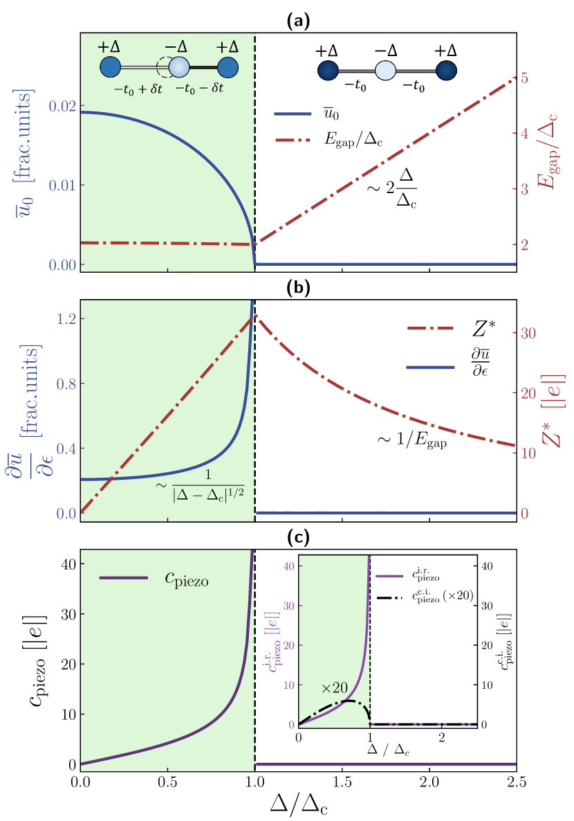
Figure 1: (a) The model presents a structural phase transition of the order parameter $\overline{u}$ with respect to the onsite energy difference $\Delta$ of neighbouring atoms. If $\Delta<\Delta_{\mathrm{c}}$ the total energy $E_{\mathrm{tot}}(u)$ has a double-well profile with two minima at $|\overline{u}|\neq 0$, resulting in a distorted chain. If $\Delta>\Delta_{\mathrm{c}}$ the minimum of $E_{\mathrm{tot}}(u)$ is in $\overline{u}=0$ and the atoms become equidistant. The behaviour of the order parameter is typical of second order phase transitions, being $\overline{u}\propto|\Delta-\Delta_{\mathrm{c}}|^{1/2}$. In the distorted phase, the energy gap $E_{\mathrm{gap}}$ is constant and it holds $E_{\mathrm{gap}}=2\Delta_{\mathrm{c}}$, while in the symmetric phase it is linearly proportional to $\Delta$. (b) The inclusion of strain $\epsilon$ in the model affects the critical value $\Delta_{\mathrm{c}}(\epsilon)$ and, as expected in a second order transition, $\overline{u}\propto|\Delta-\Delta_{\mathrm{c}}|^{-1/2}$. Near the critical point a huge polar response is also present, quantified by the effective charge $Z^{*}$. (c) In the lower-symmetry phase ($\Delta\neq 0$ and $\overline{u}\neq 0$) the piezoelectric coefficient diverges when approaching the critical point. As shown in the inset, the major contribution is due to the internal relaxation term of Equation (5). The topological nature of the enhancement guarantees its stability.

Topological contribution to the enhancement

In principle, the diverging behaviour of the strain-induced variation of $\overline{u}$, Equation (7) or (8), guarantees the existence of piezoelectric polymers with arbitrarily high response when close to a morphotropic-like phase boundary, irrespective of the prefactor, namely the effective charge $Z^{*}$. However, this specific enhancement is a consequence of the second order transition. Numerical evidence in linear acetylenic carbon chains[40] show that quantum anharmonic effects (QAE) may change the order of the structural phase transition, therefore damping the diverging behaviour of $c_{\mathrm{piezo}}^{\mathrm{i.r.}}$. A robust enhancement of the piezoelectric coefficient against QAE would depend, therefore, on the strength of the polar response embodied by $Z^{*}$. Measuring how the electronic charge distribution follows the displacement of the nuclei, effective charge’s behaviour in this system is strictly related to the topological charge transport of the Thouless pump[27]. A simple geometric argument shows that indeed the effective charge $Z^{*}$ diverges as $1/E_{\mathrm{gap}}$ (see Methods and Supplementary Information). Such a remarkable behaviour is a consequence of the topology of the domain of the dipole moment $P$[20]. As $E_{\mathrm{gap}}$ goes to $0$, we get closer to the metallic point, where $P$ is not well defined, and even an infinitesimal atomic displacement causes a huge redistribution of the charge density. We contrast this result with the predicted behaviour of polar responses in 2D gapped graphene, where both piezoelectric coefficient and effective charges were found to be independent on the band-gap amplitude[30].

The evolution of $Z^{*}$ as a function of $\Delta/\Delta_{\mathrm{c}}$ and across the transition is shown in Figure 1b). Even though the metallic divergence of the effective charge is prevented by the transition to the dimerized phase, $Z^{*}$ reaches the giant value of $\sim\!30\,|e|$ at the critical point. Unlike the MPB-related enhancement of the relaxation term, also shown in Figure 1b), the topological behaviour is expected to be much more stable with respect to QAE, guaranteeing the enhancement of the electromechanical response. The total piezoelectric coefficient, comprising both the clamped ion and internal relaxation contributions, is shown in Figure 1c) as a function of the parameter $\Delta/\Delta_{\mathrm{c}}$, while in the inset of Figure 1c) the two contributions are compared to highlight the electronic origin of the enhancement.

Numerical calculations validate predictions

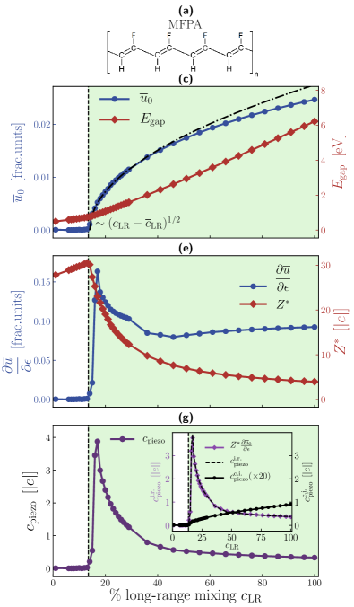
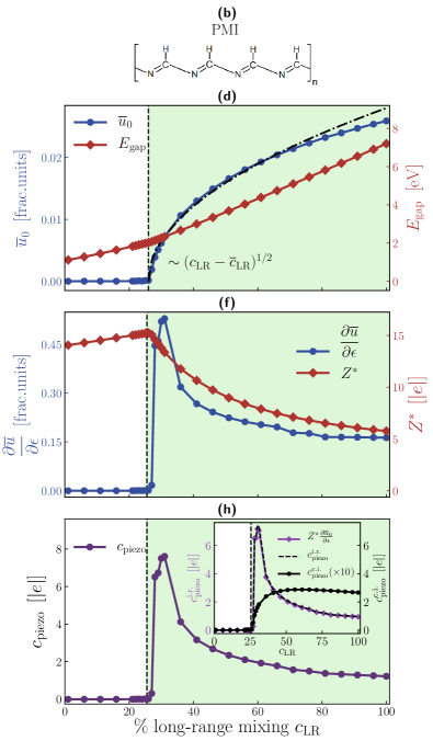
Figure 2: (a) Mono-fluorinated polyacetylene (MFPA). (b) Polymethineimine (PMI). In (c) and (d) for MFPA and PMI, respectively, is shown the behaviour of the internal coordinate $\overline{u}_{0}$ for different values of the long-range mixing parameter $c_{\mathrm{LR}}$ put in the range-separated xc-functional in the DFT calculations. Consistently with the prediction of the model, we observe the behaviour $\overline{u}\simeq|c_{\mathrm{LR}}-\overline{c}_{\mathrm{LR}}|^{1/2}$, with $\overline{c}_{\mathrm{LR}}^{\text{MFPA}}\simeq 14\%$ and $\overline{c}_{\mathrm{LR}}^{\text{PMI}}\simeq 26\%$. In (e) and (f), for MFPA and PMI respectively, the behaviour of the $\partial\overline{u}_{0}/\partial\epsilon$ is reported, along with the values of the effective charge $Z^{*}$. For each polymer, we chose $Z^{*}=Z^{*}_{C,xx}$ (for MFPA the C bound to the F). In agreement with the model, on the one hand we observe a further hint of the morphotropic-like nature of the transition while on the other hand the huge values of $Z^{*}$ stands out, in particular in the region near the critical points. In (g) and (f) is shown how the piezoelectric coefficient is greatly enhanced when reaching the critical points from the less symmetric phase. The comparison between $c_{\mathrm{piezo}}^{\mathrm{c.i.}}$ and $c_{\mathrm{piezo}}^{\mathrm{i.r.}}$, in the insets, highlights the electronic nature of the enhancement. Furthermore, the comparison with the results obtained putting the values of (e) and (f) in Equation (5) shows that the model very well describes the nature of the enhancement.

We performed ab initio calculations in the framework of Density Functional Theory (DFT) to validate our model predictions, choosing two conjugate polymers representative of the broad class of SPA. One is monofluorinated polyacetylene (MFPA) made by the repetition of the unit CH-CF, obtained by substituting one hydrogen atom of the C₂H₂ unit of PA with fluorine. The other is polymethineimine (PMI), obtained substituting a CH pair with a nitrogen atom to obtain the unit N-CH. For simplicity, we considered the all-trans structures shown in Figure 2a) and 2b), whose fundamental physical properties are captured by the Rice-Mele model. Even though controlling the fraction of substituted atoms may in principle induce a morphotropic-like transition, this approach poses many challenges both from the computational and experimental side: to our specific purposes, it wouldn’t allow to study the phase transition and the associated predicted enhancement of piezoelectric effect by varying with continuity an external parameter (as $\Delta$ in the model). As discussed in section Morphotropic-like enhancement of the piezoelectric response, the phase transition may be also tuned by the electron-phonon coupling parameter $\beta$, which in turn has been shown to depend on the dielectric environment[31, 33, 32] or on different fraction of exact exchange[40, 41]. Indeed, the asymptotic long-range Coulomb potential in a dielectric environment should be appropriately screened by the scalar dielectric constant: this requirement is met by imposing that the long-range (LR) mixing parameter $c_{\mathrm{LR}}$ – entering in range-separated hybrid (RSH) exchange-correlation functionals and accounting for the fraction of exact exchange in the long range part – is inversely proportional to the dielectric constant of the environment[42]. The enforcement of the correct asymptotic potential has been recently proved successful in the description of molecular solids within the so-called optimally tuned screened RSH approach[43, 44, 45].

Motivated by these reasons, we performed structural optimization of both MFPA and PMI for different values of the LR mixing parameter $c_{\mathrm{LR}}$. For consistency with the model, we considered the coordinates of the C and N atoms along the principal axis of the chain, which we take as the $x$-axis, to compute the internal coordinate. More details on the effect of $c_{\mathrm{LR}}$ on polymer’s structures are provided in the Supplementary Information. The evolution of $\overline{u}_{0}$ displayed in Figure 2c) and 2d), clearly hints to the presence of a second order phase transition triggered by $c_{\mathrm{LR}}$ for both polymers: the dimerized phase is suppressed by lowering the fraction of mixing, the order parameter showing the expected behaviour as it approaches the second-order phase-transition critical point. This result suggests a direct proportionality between the mixing parameter and the e-ph coupling, consistently with the expected dependence on the inverse dielectric screening in the long wavelength limit of both parameters[42, 46, 47]. In Figure 2e) and 2f) the behaviour of $Z^{*}$ and of $\partial\overline{u}/\partial\epsilon$ calculated from first principles is shown. For MFPA we took $Z^{*}=Z^{*}_{C_{F},xx}$ where $C_{F}$ is the carbon atom bound to the fluorine, while for PMI $Z^{*}=Z^{*}_{C,xx}$. The full tensors of the effective charges of all the atoms are reported in the Supplementary Information. We highlight the qualitative agreement with the prediction of the model, in particular the huge enhancement of the effective charges around the critical point $\overline{c}_{\mathrm{LR}}$, reaching the strongly anomalous values of $\sim\!\!30\,|e|$ and $\sim\!\!15\,|e|$ in correspondence of $\overline{c}_{\mathrm{LR}}$ for MFPA and PMI, respectively. The covalent character of bonds along the chain prevents a precise definition of the nominal reference value for C, that can be however assumed to be of the order of $1|e|$, as the nominal ionic charges for H and F are respectively $+1|e|$ and $-1|e|$. Effective charges of carbon in both considered chains are strongly anomalous for all considered long-range mixing parameters, displaying values between $5|e|$ and $30|e|$ even for band gaps exceeding 6 eV. These anomalous values exceed even those reported in oxide ferroelectrics, where effective charges are typically two or three times larger than nominal reference values[48]. Figure 2g) and 2h) display the behaviour of the piezoelectric coefficients computed ab initio taking into account also the effects of transverse displacements. In the insets, the different contributions $c_{\mathrm{piezo}}^{\mathrm{i.r.}}$ and $c_{\mathrm{piezo}}^{\mathrm{c.i.}}$ are compared, highlighting the electronic origin of the enhancement. Using the the ab initio values of $Z^{*}$ and $\partial\overline{u}/\partial\epsilon$ of Figure 2e) and 2f), we compare the values of $c_{\mathrm{piezo}}^{\mathrm{i.r.}}$ computed without approximations with those obtained using Equation (5) of the model. The agreement between the two approaches is both qualitatively and quantitatively excellent, notwithstanding the simplifying description provided by the Rice-Mele model, that neglects structural details specific of the two considered polymers as well as transverse displacements. We highlight that despite the behaviour $\partial\overline{u}/\partial\epsilon\propto|c_{\mathrm{LR}}-\overline{c}_{\mathrm{LR}}|^{-1/2}$, the main contribution to the piezoelectric coefficient is given by the effective charges. The large values attained in a finite range around the second-order critical point and their ultimately topological origin suggest that the piezoelectric effect is robust against quantum and anharmonic effects that may change the order of the phase transition, as predicted in carbyne[40].

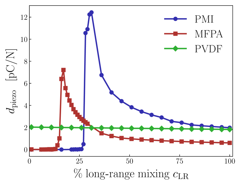
Figure 3: Comparison of the converse piezoelectric coefficients of MFPA and PMI with respect to PVDF, the current best and most widely used organic piezoelectric. In principle, the mechanism of the morphotropic-topological enhancement allows to outperform the state-of-the-art.

Discussion

Finally, we compare the results for the piezoelectric coefficients of MFPA and PMI with those of the best and most widely used piezoelectric PVDF polymer, made by the repetition of the unit CF₂-CH₂. The Rice-Mele model fails to capture its main properties, this polymer being not conjugated. Its piezoelectricity indeed derives from the presence of a net dipole moment transverse to the chain, whereas the electromechanical response predicted in conjugated polymers is longitudinal to the chain and ultimately due to the topological-morphotropic enhancement. To have a consistent comparison with available experimental data for PVDF, we computed ab initio the converse piezoelectric coefficient $d_{\mathrm{piezo}}$, which measures the response with respect to an external stress, rather than a strain, being linearly related to $c_{\mathrm{piezo}}$ through the elastic constants tensor $\mathbb{C}$, namely $c_{\mathrm{piezo}}=d_{\mathrm{piezo}}\mathbb{C}$. As far as 1D systems are concerned, only a single scalar elastic constant is required, and it can be evaluated as the second derivative of the energy with respect to the strain, i.e. $\mathbb{C}=\partial^{2}E/\partial\epsilon^{2}$. The results for the converse piezoelectric coefficients of PVDF are compared with those of MFPA and PMI in Figure 3 and are consistent with the values computed in Ref. [49]. Even though the calculated $d_{\mathrm{piezo}}$ is smaller than reported experimental values, a direct comparison to experiments is hardly drawn because, e.g., of the polymorphic character or low crystallinity of experimental samples, as noticed also in Ref. [49]. We remark that piezoelectric response in PVDF is found to be independent on the fraction of exact exchange, confirming the utterly different nature of the electromechanical response in such non-conjugated polymer. We finally mention that mildly anomalous effective charges have been also reported for PVDF[50], the carbon effective charge however not exceeding 1.5$|e|$, consistently with our results provided in Supplementary Information. On the other hand, both MFPA and PMI display a rather large range of values that are larger than calculated $d_{\mathrm{piezo}}$ of PVDF, with up to a six-fold enhancement for PMI close to the dimerization point. Even though the selected prototypical SPAs may not be the most efficient ones for practical realization and engineering of their functional properties, the comparison with first-principles estimate of one of the best available piezoelectric polymer alongside the general validity of the proposed model and consequent robustness of its electromechanical response put forward the broad class of $\pi$-conjugated polymers as a promising field for organic piezoelectrics with enhanced functionalities. Additionally, its inverse proportionality to the band gap provides a possible material-design principle for driving the quest of organic polymers with enhanced piezoelectric response.

Methods

Details on the model

The Hamiltonian of the chain is the sum of two terms $H_{\mathrm{tot}}=H_{\mathrm{L}}+H_{\mathrm{e}}$. The lattice contribution $H_{\mathrm{L}}$ accounts for the displacement of the atoms with respect to their position in a uniformly spaced chain:

$$H_{\mathrm{L}}=\sum_{i}\frac{p_{i}^{2}}{2m_{i}}+\frac{1}{2}\mathrm{K}\sum_{i}(\delta r_{i+1}-\delta r_{i})^{2}$$ (9)

where $m_{i}$ and $\delta r_{i}$ are mass and displacement of atom $i$, $p_{i}$ its momentum, and $\mathrm{K}$ is a spring constant term. In a nearest neighbours tight-binding approximation, the electronic contribution $H_{\mathrm{e}}$ reads

$$H_{\mathrm{e}}=2\sum_{i}\left[\Delta(-1)^{i}c_{i}^{\dagger}c^{\phantom{\dagger}}_{i}-\left(t_{i,i+1}c_{i}^{\dagger}c^{\phantom{\dagger}}_{i+1}+\mathrm{h.c.}\right)\right],$$ (10)

where the factor $2$ accounts for the spin degeneracy, $c_{i}^{\dagger}$/$c_{i}$ are creation/annihilation operators for electrons, $t_{i,i+1}$ is a hopping energy while $\Delta>0$ accounts for the onsite energy difference between neighbours. The adimensional order parameter $u(\epsilon)$ measures the relative displacement between neighbours and is defined as

$$u(\epsilon)=\frac{\delta r_{i+1}(\epsilon)-\delta r_{i}(\epsilon)}{a(\epsilon)/2}.$$ (11)

The total energy of the system $E_{\mathrm{tot}}(u)$ as a function of the order parameter $u$ has two contributions, namely

$$E_{\mathrm{tot}}(u)=E_{\mathrm{L}}(u)+E_{\mathrm{e}}(u).$$ (12)

The first term $E_{\mathrm{L}}(u)$ accounts for lattice distortion and is quadratic in $u$, whereas the electronic contribution $E_{\mathrm{e}}(u)$ is linear in $u$. For a given set of material-dependent parameter $t_{0}$, $\mathrm{K}$, $\Delta$, $\beta$ and the strain $\epsilon$, we find the optimal displacement $\overline{u}$ – defined as the one which minimises the total energy – as shown in detail in the Supplementary Information.

We computed the dipole moment per unit cell $P$ using the Berry phase approach[51, 52]. In the limit $E_{\mathrm{gap}}\ll t(\epsilon)$ it holds (see Supplementary Information)

$$P(\epsilon,\overline{u}(\epsilon))=-\frac{|e|}{\pi}\theta(\epsilon,\overline{u}(\epsilon))$$ (13)

with $\tan\theta(\epsilon,\overline{u}(\epsilon))=\Delta/2\delta t(\epsilon,\overline{u}(\epsilon))$, where we emphasize that the dependence on the strain enters both directly and through $\overline{u}(\epsilon)$. Using Equation (2) and (13) we have

$$c_{\mathrm{piezo}}^{\mathrm{c.i.}}=-\frac{|e|}{2\pi}\beta\sin 2\theta(0,\overline{u}_{0})$$ (14)

where we notice that $|c_{\mathrm{piezo}}^{\mathrm{c.i.}}|\leq|e|\beta/2\pi$, the maximum achievable value being directly proportional to the e-ph coupling constant $\beta$.

Plugging Equation (2) in Equation (13), we obtain an explicit expression for the effective charge in both the dimerized and undimerized phases:

$$Z^{*}(\overline{u}_{0}) =\frac{|e|}{\pi}4\beta t_{0}\frac{\sin\theta(0,\overline{u}_{0})}{E_{\mathrm{gap}}(0,\overline{u}_{0})}.$$ (15)

where we highlight the presence of the term $E_{\mathrm{gap}}$ at the denominator. The diverging behaviour as $1/E_{\mathrm{gap}}$ can be also derived directly using a simple geometric argument. As highlighted in Equation (13), polarization is proportional to an angle $\theta$ spanning the parametric ($\Delta,\delta t$)-space along a circumference with radius $E_{\mathrm{gap}}$. As $\delta t\propto u$, it follows that in the undimerized phase $E_{\mathrm{gap}}d\theta\propto du$, hence $Z^{*}=\partial P/\partial u\propto\partial\theta/\partial u\propto 1/E_{\mathrm{gap}}$ (more details in the Supplementary Information).

The parameters used to produce the results in Figure 1 were obtained fitting the model with the PBE0[53] total energy profile of carbyne as a function of the relative displacement of the two carbon atoms of its unit cell. In particular, with the value $a_{0}=2.534$ Š obtained through a cell-relaxation procedure, the fit yields $t_{0}=2.239$ eV, $\beta=3.906$ and $\mathrm{K}=127.9$ eV/Ų, whereas for carbyne it holds $\Delta=0$. We highlight that each carbon atom of carbyne contributes with two electrons to the $\pi$-orbital, so it is necessary to put an additional factor of $2$ in front of Equation (10) to account for this degeneracy.

Computational details

All DFT calculations were performed using CRYSTAL simulation code[54, 55]. We used a triple-$\zeta$-polarised gaussian type basis[56] with real space integration tolerances of 10-10-10-15-30 and an energy tolerance of $10^{-10}$ Ha for the total energy convergence. We customised a range-separated LC-$\omega$PBE hybrid exchange-correlation functional[57] varying the value of the long-range (LR) mixing parameter $c_{\mathrm{LR}}$ which enters in the definition of the LR part of the functional, namely

$$E_{\mathrm{xc}}^{\mathrm{LC-}\omega\mathrm{PBE}}=E_{\mathrm{xc}}^{\mathrm{PBE}}+c_{\mathrm{LR}}\left(E_{\mathrm{x}}^{\mathrm{LR,HF}}-E_{\mathrm{x}}^{\mathrm{LR,PBE}}\right).$$ (16)

When $c_{\mathrm{LR}}=0$ the PBE functional is recovered while if $c_{\mathrm{LR}}=1$ we have pure Hartree-Fock (HF) exchange. The long-range terms in round brackets depend on the range-separation parameter $\omega$ that enters in the decomposition of the Coulomb operator $1/r$ as

$$\frac{1}{r}=\frac{1-\mathrm{erf}(\omega r)}{r}+\frac{\mathrm{erf}(\omega r)}{r}$$ (17)

where $\mathrm{erf}(\cdot)$ is the error function; the first and second term in the right-hand side of Eq. 17 account for the short- and long-range part of the Coulomb operator, respectively. All the presented values were obtained with $\omega=0.4$ a${}_{0}^{-1}$. For each $c_{\mathrm{LR}}$, a geometric optimisation was performed and all quantities were computed on the equilibrium configurations (see Supplementary Information). The derivatives $\partial\overline{u}/\partial\epsilon$ of the order parameter with respect to the strain were computed with finite differences, performing a fixed-cell optimisation for each strained configuration with cell length $a(\epsilon)=a_{0}(1\pm\epsilon)$ and $\epsilon=0.01$, while the effective charges were computed with a vibrational frequency calculation[58]. The piezoelectric coefficients $c_{\mathrm{piezo}}$ and $d_{\mathrm{piezo}}$ of Figure 2g), 2h) and 3, as well as the values of $c_{\mathrm{piezo}}^{\mathrm{c.i.}}$ and of $c_{\mathrm{piezo}}^{\mathrm{i.r.}}$, were computed using the Berry-phase approach[59] implemented in the code[60, 61], which accounts also for transverse displacements.

Supplementary Information

Inclusion of strain in the Rice-Mele model

In this section we provide a detailed description of the Rice-Mele model[22] and the proposed extension that enables the description of strain effects. We consider an infinitely long one-dimensional linear chain made by the repetition of a unit cell, of length $a_{0}$, containing two atoms: one of type $A$ and the other of type $B$. We recall that the only possible strains in 1D are contractions or dilatations of the unit cell. Defining the adimensional parameter $\epsilon$, the effect of strain on the unit cell length $a_{0}$ is

$$a(\epsilon)=a_{0}(1+\epsilon).$$ (S1)

Electronic properties of the system are described in a nearest-neighbour tight-binding approximation. We assume one electronic orbital per atom, e.g., the $p$-orbital of carbon atoms, and we adopt the notation $\ket{\alpha,R}$ to indicate that the orbital of atom $\alpha=A,B$ is located at $r_{\alpha}+R$, $R=na$ ($n\in\mathbb{Z}$) being the position of the atom’s cell along the chain. Without loss of generality, we take $r_{A}=-a/4+\delta r_{A}$ and $r_{B}=+a/4+\delta r_{B}$, $\delta r_{\alpha}$ being the displacement of atom $\alpha$. For simplicity, we consider only longitudinal displacements, parallel to the linear-chain direction. The basis set of the orbitals $\{\ket{\alpha,R}\}$ is orthonormal and it holds:

$$\Braket{\alpha,R}{\alpha^{\prime},R^{\prime}}=\delta_{\alpha,\alpha^{\prime}}\delta_{R,R^{\prime}}.$$ (S2)

We define the onsite energy terms of the electronic Hamiltonian $H_{\mathrm{e}}$ as

$$\Braket{A,R}{H_{\mathrm{e}}}{A,R^{\prime}}=-\Braket{B,R}{H_{\mathrm{e}}}{B,R^{\prime}}=-\Delta\delta_{R,R^{\prime}},\;\mathrm{with}\;\;\Delta\geq 0.$$ (S3)

We take into account also the energetic contribution due to the overlap between an atom’s orbital and the orbitals of its left and right nearest neighbours. In general, the overlap energy term between two electronic orbitals is a function of the distance $r$ between the atoms and is referred to as the hopping energy $-t(r)$, $t>0$. For convenience, we indicate with $r_{1}$ the distance between atoms in the same cell and with $r_{2}$ the distance between neighbouring atoms in adjacent cells, namely:

$$r_{1} \equiv(r_{B}+R)-(r_{A}+R)=\frac{a}{2}+\delta r_{B}-\delta r_{A},$$ (S4)

$$r_{2} \equiv(r_{A}+R)-(r_{B}+R-a)=\frac{a}{2}+\delta r_{A}-\delta r_{B}$$ (S5)

and it holds $r_{1}+r_{2}=a$. We can now define the hopping energy between orbitals of atoms in the same cell $-t_{1}\equiv-t(r_{1})$ and the hopping energy between atoms in adjacent cells $-t_{2}\equiv-t(r_{2})$. With the same notation of Equation (S3) we write:

$$\Braket{A,R}{H_{\mathrm{e}}}{B,R^{\prime}}=\Braket{B,R^{\prime}}{H_{\mathrm{e}}}{A,R}^{*}=-t_{1}\delta_{R,R^{\prime}}-t_{2}\delta_{R-a,R^{\prime}}.$$ (S6)

As we are interested in the effects of strain $\epsilon$ and of atoms’ displacement, we define, using Equation (S4) and (S5), an adimensional fractional coordinate $u(\epsilon)$:

$$u(\epsilon)=\frac{r_{1}-r_{2}}{a(\epsilon)}=\frac{\delta r_{B}-\delta r_{A}}{a(\epsilon)/2}.$$ (S7)

This term quantifies deviations from the equally spaced chain, allowing us to express bond lengths with the following compact expression:

$$r_{i}=\frac{a(\epsilon)}{2}\left[1+(-1)^{i+1}u(\epsilon)\right],\;i=1,2.$$ (S8)

With the above definitions, at linear order in atoms’ displacement we have

$$t_{i}=t(r_{i})\simeq t\left(\frac{a(\epsilon)}{2}\right)+\left.\frac{\mathrm{d}t}{\mathrm{d}r}\right|_{\frac{a(\epsilon)}{2}}\cdot\left(r_{i}-\frac{a(\epsilon)}{2}\right),$$ (S9)

which allow us to define the two terms

$$t(\epsilon) =\frac{t_{1}+t_{2}}{2},$$ (S10)

$$\delta t(\epsilon) =\frac{t_{1}-t_{2}}{2}.$$ (S11)

The former term $t(\epsilon)$ quantifies the effect of strain on the hopping energy between equidistant atoms while the latter term $\delta t(\epsilon)$ describes the variation with respect to $t(\epsilon)$ caused by atoms’ relative displacement. In absence of strain ($\epsilon=0$) we recover the quantities defined in the Rice-Mele model, whereas at linear order in $\epsilon$ it holds:

$$t\left(\epsilon\right) =t\left(\frac{a_{0}}{2}(1+\epsilon)\right)\simeq t\left(\frac{a_{0}}{2}\right)+\left.\frac{\mathrm{d}t}{\mathrm{d}r}\right|_{\frac{a_{0}}{2}}\cdot\left.\frac{\mathrm{d}a(\epsilon)}{\mathrm{d}\epsilon}\right|_{\epsilon=0}\cdot\frac{\epsilon}{2}=$$ (S12)

$$=t_{0}(1-\beta\epsilon)$$ (S13)

where $t_{0}\equiv t(a_{0}/2)$ and we defined the adimensional parameter $\beta>0$ as

$$\beta\equiv-\frac{a_{0}}{2t_{0}}\left.\frac{\mathrm{d}t}{\mathrm{d}r}\right|_{\frac{a_{0}}{2}}.$$ (S14)

This term quantifies the variation of the hopping energy due to a variation of the distance between the atoms and as such it acts as an electron-phonon coupling term. Analogously, we obtain

$$\delta t(\epsilon)=-t_{0}\beta^{\prime}(1+\epsilon)u(\epsilon),$$ (S15)

where we define another adimensional e-ph parameter $\beta^{\prime}>0$ as

$$\beta^{\prime}=-\frac{a_{0}}{2t_{0}}\left.\frac{\mathrm{d}t}{\mathrm{d}r}\right|_{\frac{a(\epsilon)}{2}}.$$ (S16)

Even though the two e-ph parameters $\beta^{\prime}$, $\beta$ can differ at finite values of the strain, at the lowest order one can safely assume that they coincide and consider $\beta^{\prime}=\beta$. A schematic representation of the model is shown as an inset in Figure S2.

Structural phase transition

As we are interested in the structural properties at $T=0~{}K$, we study the total energy per unit cell $E_{\mathrm{tot}}(u)=E_{\mathrm{L}}(u)+E_{\mathrm{e}}(u)$, where $E_{\mathrm{L}}(u)$ and $E_{\mathrm{e}}(u)$ are the lattice and electronic contribution, respectively. In particular, we aim to characterise the behaviour of the optimal displacement $\overline{u}$, defined as the one which minimises $E_{\mathrm{tot}}(u)$ given a set of material-dependent parameters $t_{0}$, $\mathrm{K}$, $\Delta$, $\beta$ and a strain $\epsilon$. Lattice dynamics being neglected, we write the lattice contribution, which accounts for the displacement of the atoms with respect to their position in a uniformly spaced chain:

$$E_{\mathrm{L}}(u)=\frac{1}{2}\mathrm{K}\left(\delta r_{A}-\delta r_{B}\right)^{2}+\frac{1}{2}\mathrm{K}\left(\delta r_{B}-\delta r_{A}\right)^{2}=\frac{1}{4}\mathrm{K}a^{2}(\epsilon)u^{2}(\epsilon),$$ (S17)

where we used Equation (S7) and $\mathrm{K}$ is an elastic constant term.

To compute the electronic energy per unit cell $E_{\mathrm{e}}(u)$, we imagine the linear chain as made of $N$ copies of the unit cell and we adopt periodic boundary conditions. This allows us to define a basis $\{\ket{\alpha,k}\}$ in the reciprocal $k$-space:

$$\ket{\alpha,k}\equiv\sum_{R}\frac{\mathrm{e}^{\mathrm{i}\left(r_{\alpha}+R\right)k}}{\sqrt{N}}\ket{\alpha R},$$ (S18)

where $k$ is defined over the first Brillouin zone, namely

$$k=\frac{n}{N}\frac{2\pi}{a},\;\;\;n=0,\pm\frac{1}{2},\pm 1,\dots,\pm\frac{N}{2},$$ (S19)

and it holds

$$\Braket{\alpha^{\prime},k^{\prime}}{\alpha k}=\delta_{\alpha,\alpha^{\prime}}\delta_{k,k^{\prime}}.$$ (S20)

From Equation (S3), (S6) and (S18) we obtain the matrix elements of the electronic Hamiltonian in the reciprocal space:

$$\Braket{A,k}{H_{\mathrm{e}}}{A,k^{\prime}} =-\Delta\delta_{k,k^{\prime}},$$ (S21)

$$\Braket{B,k}{H_{\mathrm{e}}}{B,k^{\prime}} =\Delta\delta_{k,k^{\prime}},$$ (S22)

$$\Braket{A,k}{H_{\mathrm{e}}}{B,k^{\prime}} =-t_{1}\mathrm{e}^{\mathrm{i}\frac{a}{2}k}\mathrm{e}^{\mathrm{i}k\left(\delta r_{B}-\delta r_{A}\right)}\delta_{k,k^{\prime}}-t_{2}\mathrm{e}^{-\mathrm{i}\frac{a}{2}k}\mathrm{e}^{\mathrm{i}k\left(\delta r_{B}-\delta r_{A}\right)}\delta_{k,k^{\prime}}\equiv-T\delta_{k,k^{\prime}},$$ (S23)

$$\Braket{B,k}{H_{\mathrm{e}}}{A,k^{\prime}} =\Braket{A,k^{\prime}}{H_{\mathrm{e}}}{B,k}^{*}=-T^{*}\delta_{k,k^{\prime}}.$$ (S24)

The above results allow to write in the reciprocal space basis a $2\times 2$ electronic Hamiltonian matrix $H_{\mathrm{e},k}$ for each $k$-point:

$$H_{\mathrm{e},k}=\begin{pmatrix}-\Delta&-T\\ -T^{*}&\Delta\end{pmatrix}.$$ (S25)

Diagonalising the matrix of Equation (S25) we find the two eigenvalues

$$\varepsilon_{k}^{\pm}=\pm\sqrt{\Delta^{2}+|T|^{2}}$$ (S26)

with the respective eigenvectors, namely the Bloch wave-functions

$$\ket{\psi_{k}^{\pm}}=\begin{pmatrix}\frac{\pm\left(\varepsilon_{k}^{\pm}-\Delta\right)}{\sqrt{\left(\varepsilon_{k}^{\pm}-\Delta\right)^{2}+|T|^{2}}}\\ \frac{-T^{*}}{\sqrt{\left(\varepsilon_{k}^{\pm}-\Delta\right)^{2}+|T|^{2}}}\end{pmatrix},$$ (S27)

and using Equation (S10), (S11) and S23 we have that

$$|T|^{2}=4t^{2}\cos^{2}k\frac{a}{2}+4\delta t^{2}\sin^{2}k\frac{a}{2}.$$ (S28)

For each $k$-point, Equation (S26) allows to distinguish between a lower and a higher energy level. As shown in Figure S1, the chain present two energy bands. To describe the $\pi-$orbitals of conjugated orbitals, we assume that only the lower energy band is filled with electrons and will hereafter refer to it as the occupied band, in contrast with the unoccupied higher energy band. From Equation (S26) we obtain the value of the energy gap $E_{\mathrm{gap}}$ between the occupied and unoccupied band:

$$E_{\mathrm{gap}}=\sqrt{(4\delta t)^{2}+(2\Delta)^{2}}.$$ (S29)

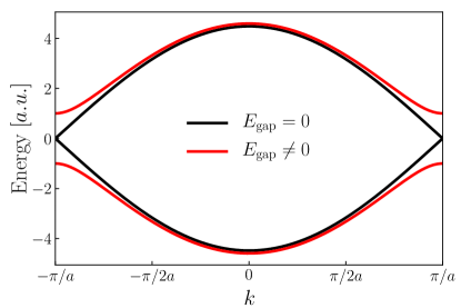
Figure S1: Electronic bands structure of the model. If $E_{\mathrm{gap}}=0$, the bands have linear dispersion at the edges of the Brillouin zone, reminding the behaviour of graphene. To describe the properties of conjugated polymers, we assume that only the lower energy bands are occupied with electrons.

We consider the contribution of all the occupied states to the electronic energy per unit cell and in particular it holds

$$E_{\mathrm{e}}=\frac{2}{N}\sum_{k}\varepsilon_{k}^{-}=-\frac{2}{N}\sum_{k}\sqrt{\Delta^{2}+4t^{2}\cos^{2}\frac{ka}{2}+4\delta t^{2}\sin^{2}\frac{ka}{2}}$$ (S30)

where the factor of $2$ accounts for the spin degeneracy. In the limit of an infinite linear chain, namely for $N\to+\infty$, the eigenvalues and the eigenvectors’ coefficients become continuous functions of $k$ and the sum becomes an integral over the first Brillouin zone:

$$E_{\mathrm{e}}=-2a\int_{-\pi/a}^{\pi/a}\frac{\mathrm{d}k}{2\pi}\sqrt{\Delta^{2}+4t^{2}\cos^{2}\frac{ka}{2}+4\delta t^{2}\sin^{2}\frac{ka}{2}}.$$ (S31)

Finally, using Equation (S15), (S17) and (S31), we write the total energy per unit cell as a function of the fractional coordinate $u$:

$$E_{\mathrm{tot}}(u)=\frac{1}{4}\mathrm{K}u^{2}a(\epsilon)^{2}-2a\int_{-\pi/a}^{\pi/a}\frac{\mathrm{d}k}{2\pi}\sqrt{\Delta^{2}+4t^{2}(\epsilon)\cos^{2}\frac{ka}{2}+4\beta^{2}t_{0}^{2}(1+\epsilon)^{2}u^{2}\sin^{2}\frac{ka}{2}}.$$ (S32)

We can now study the structural properties of the system, encompassed in the optimal displacement $\overline{u}$, defined as the one which minimises $E_{\mathrm{tot}}(u)=E_{\mathrm{L}}(u)+E_{\mathrm{e}}(u)$ given a set of material-dependent parameters $t_{0}$, $\mathrm{K}$, $\Delta$, $\beta$ and a strain $\epsilon$. With the substitution $z=ka/2$ and exploiting the parity of the integrand in Equation (S32), the first derivative of the total energy with respect to $u$ reads:

$$\frac{\mathrm{d}E_{\mathrm{tot}}}{\mathrm{d}u}=\frac{1}{2}\mathrm{K}a^{2}(\epsilon)u-\frac{1}{\pi}\int_{-\pi/2}^{0}\mathrm{d}z\frac{16\beta^{2}t_{0}^{2}(1+\epsilon)^{2}u\sin^{2}z}{\sqrt{\Delta^{2}+4t^{2}(\epsilon)\cos^{2}z+4\beta^{2}t_{0}^{2}(1+\epsilon)^{2}u^{2}\sin^{2}z}}.$$ (S33)

One of the stationary point of Equation (S33) is in $u=0$, whereas the others are the solutions of the following equation in $u$:

$$\mathrm{K}a^{2}(\epsilon)\pi=\int_{-\pi/2}^{0}\mathrm{d}z\frac{32\beta^{2}t_{0}^{2}(1+\epsilon)^{2}\sin^{2}z}{\sqrt{\Delta^{2}+4t^{2}(\epsilon)\cos^{2}z+4\beta^{2}t_{0}^{2}(1+\epsilon)^{2}u^{2}\sin^{2}z}}.$$ (S34)

To solve this integral, we expand the functions $\sin z$ and $\cos z$ at the lower edge of the Brillouin zone, namely in $k=-\pi/a$, in a similar fashion to the conic approximation in graphene. By doing so, we arrive at

$$\Delta^{2}+4\beta^{2}t_{0}^{2}(1+\epsilon)^{2}u^{2}=\frac{t_{0}^{2}(1-\beta\epsilon)^{2}\pi^{2}}{\sinh^{2}\frac{\mathrm{K}a_{0}^{2}\pi(1-\beta\epsilon)}{8\beta^{2}t_{0}}}.$$ (S35)

Supposing that $\Delta$ is the parameter which guides the transition, we define

$$\Delta_{\mathrm{c}}=\frac{t_{0}(1-\beta\epsilon)\pi}{\sinh\left(\frac{\mathrm{Ka_{0}^{2}\pi(1-\beta\epsilon)}}{16\beta^{2}t_{0}}\right)}.$$ (S36)

As we are interested in the real solutions only, the above equations tells that if $\Delta\leq\Delta_{\mathrm{c}}$, the solution of Equation (S35) provides two symmetric stationary points for $E_{\mathrm{tot}}(u)$. Indicating with $\overline{u}$ the value which minimises $E_{\mathrm{tot}}(u)$, it is straightforward to verify, e.g. computing the second order derivative of $E_{\mathrm{tot}}(u)$, that

$$\begin{cases}\overline{u}\propto|\Delta-\Delta_{\mathrm{c}}|^{1/2},&\;\mathrm{if}\;\Delta\leq\Delta_{\mathrm{c}}\\ \overline{u}=0,&\;\mathrm{if}\;\Delta>\Delta_{\mathrm{c}}.\end{cases}$$ (S37)

Moreover, it is also immediate to verify that the second order derivative of $E_{\mathrm{tot}}(u)$ computed at $u(\Delta_{\mathrm{c}})=0$ is a saddle point. These results show that the chain undergoes a second order phase transition in $\Delta$ with $\overline{u}$ as order parameter: when $\Delta>\Delta_{\mathrm{c}}$, the atoms are equidistant ($\overline{u}=0$), while for $\Delta\leq\Delta_{\mathrm{c}}$ the chain displays a bond length alternation that breaks the inversion symmetry of the cell. Figure S2 displays two representative energy profiles, one for each phase, obtained from Equation (S32): the two minima of a double-well energy landscape in the distorted phase collapse into a single minimum when $\Delta\geq\Delta_{\mathrm{c}}$, i.e., when the local maximum at $u=0$ turns into a global minimum, signature of the second order transition. It is interesting to notice that the left-hand side of Equation (S35) is equal to $E^{2}_{\mathrm{gap}}/4$, implying that in the distorted phase, as $\Delta$ varies, $\overline{u}(\Delta)$ varies in a way that keeps the energy gap constant. Stated in other words, the knowledge of the energy gap gives also information on the phase diagram of the system and vice versa. However, the parameter $\Delta$ is not the only handle available to drive the transition, that may be tuned by other model parameters at fixed $\Delta$. For instance, it is reasonable that a sufficiently large e-ph coupling may induced bond dimerization in the gapped chain at finite $\Delta$. The optimal $\bar{u}\neq 0$ as a function of $\beta$ is given in closed form in Equation (S35). As the e-ph coupling constant enters in the hyperbolic function, an explicit expression for $\bar{u}$ can be derived by assuming $\mathrm{K}a_{0}^{2}\pi(1-\beta\epsilon)\ll 8\beta^{2}t_{0}$, which allows to retain only the lowest order term of the Taylor expansion of $\sinh(x)$. With this hypothesis, and defining the term

$$\beta_{\mathrm{c}}^{2}=\frac{\mathrm{K}a_{0}^{2}}{8t_{0}^{2}}\Delta,$$ (S38)

in analogy with the previous case, we obtain

$$\begin{cases}\overline{u}\propto|\beta-\beta_{\mathrm{c}}|^{1/2},&\;\mathrm{if}\;\beta<\beta_{\mathrm{c}}\\ \overline{u}=0,&\;\mathrm{if}\;\beta\geq\beta_{\mathrm{c}}.\end{cases}$$ (S39)

This result shows that another way to control the structure of the chain in the Rice-Mele model, namely given a finite $\Delta\neq 0$, is through the electron-phonon coupling term $\beta$.

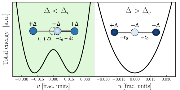
Figure S2: Behaviour of the total energy per unit cell $E_{\mathrm{tot}}$ with respect to the fractional coordinate $u$. If $\Delta\leq\Delta_{\mathrm{c}}$, there are two symmetric minima $\overline{u}\neq 0$ and the equilibrium structure present a bond length alternation. If $\Delta>\Delta_{\mathrm{c}}$, there is only one minimum in $\overline{u}=0$ and the atoms are equidistant.

Electronic polarization and Thouless pump

In this section, we derive the expression of the dipole moment per unit cell $P$ as obtained within the modern theory of polarization[51]. In this framework, the wave function of the occupied states is required to be continuous at the edges of the Brillouin zone. To satisfy the requirement, we multiply the wave function for the occupied states of Equation (S27) by a phase factor and define

$$\ket{\psi_{k}^{\mathrm{occ}}}\equiv\mathrm{e}^{-\mathrm{i}r_{A}k}\ket{\psi_{k}^{-}}$$ (S40)

with $r_{A}=-a/4+\delta r_{A}$. The dipole moment per unit cell $P$ is defined in term of the Berry phase[62] $\varphi$ as

$$P=\frac{-2|e|}{2\pi}\varphi$$ (S41)

where $e$ is the electron’s charge, the factor $2$ at the numerator accounts for the spin degeneracy and the Berry phase $\varphi$ is defined as

$$\varphi=\mathrm{i}\int_{-\pi/a}^{\pi/a}\mathrm{d}k\Braket{\widetilde{\psi}_{k}^{\mathrm{occ}}}{\frac{\mathrm{d}\widetilde{\psi}_{k}^{\mathrm{occ}}}{\mathrm{d}k}}.$$ (S42)

We indicated with $\ket{\widetilde{\psi}_{k}^{\mathrm{occ}}}$ the periodic part of the wave function $\ket{\psi_{k}^{\mathrm{occ}}}$ and from Equation (S18), (S27) and (S40) it holds

$$\ket{\widetilde{\psi}_{k}^{\mathrm{occ}}}=\mathrm{e}^{-\mathrm{i}r_{A}k}\sum_{R}\sum_{\alpha}c_{\alpha,k}\ket{\alpha R},$$ (S43)

where

$$c_{A,k} =\frac{\Delta-\varepsilon_{k}^{-}}{\sqrt{\left(\Delta-\varepsilon_{k}^{-}\right)^{2}+|T|^{2}}},$$ (S44)

$$c_{B,k} =\frac{-T^{*}}{\sqrt{\left(\Delta-\varepsilon_{k}^{-}\right)^{2}+|T|^{2}}}.$$ (S45)

As the scalar product in Equation (S42) is taken over a single unit cell, without loss of generality we consider only the contribution for $R=0$ in Equation (S43) and obtain

$$\varphi=\frac{2\pi}{a}r_{A}+\int_{\pi/a}^{\pi/a}\mathrm{d}k\frac{\left(\delta r_{B}-\delta r_{A}\right)|T|^{2}+2t\delta ta}{(\Delta-\varepsilon_{k}^{-})^{2}+|T|^{2}}.$$ (S46)

From the gap Equation (S29), we notice that the insulating/metallic character of the system can be visualised in a 2D parametric $(\Delta,\delta t)-$space, where the origin of the axes correspond to a metallic system with $E_{\mathrm{gap}}=0$, while every other point correspond to an insulating system with $E_{\mathrm{gap}}\neq 0$. In this space, we define a parameter $\theta$ that allows to identify each point with the polar coordinates $(E_{\mathrm{gap}},\theta)$, with the change of coordinates defined by

$$2\Delta =E_{\mathrm{gap}}\sin\theta$$ (S47)

$$4\delta t =E_{\mathrm{gap}}\cos\theta.$$ (S48)

Applying this change of coordinates in Equation (S46), in the limit $E_{\mathrm{gap}}\ll t_{0}$ it can be demonstrated that it holds

$$P=-\frac{|e|}{\pi}\theta.$$ (S49)

This property can be appreciated in Figure S3, where we compare, for different values of $E_{\mathrm{gap}}/t_{0}$, the behaviour with respect to $\theta$ of the dipole moment $P$, obtained computing Equation (S41) numerically without further approximations. As $\theta$ varies, so do the terms $\Delta$ and $\delta t$. In particular, a full rotation of $2\pi$ implies that the system has returned in its initial state, while the dipole moment $P$ has acquired a quantum of $-2|e|$. This properties is more general: if the system undergoes an adiabatic evolution along any loop enclosing the origin of the 2D space, a quantised charge is always pumped out. This phenomenon is known as adiabatic charge transport or Thouless’ pump[27] and the key ingredient is the presence of the metallic point in the domain enclosed by the loop: in this sense, it is an example of topological phenomenon. This peculiar topology-related property has consequences also in the behaviour of the effective charges of the system. Defined as the variation of polarization due to an atomic displacement, the effective charges are a measure of how rigidly the electronic charge distribution follows the displacement of the nuclei. In the model it holds

$$Z^{*}=\frac{\partial P}{\partial u}.$$ (S50)

With the definitions given above one can compute analytically the expression for $Z^{*}$, however it is possible to appreciate the main feature of its behaviour thanks to a geometric argument in the ($\Delta,\delta t$)-space. The effect of a small displacement on a system with a finite $\Delta\neq 0$ is to span an angle $\mathrm{d}\theta$ in the space, starting from $\theta=\pi/2$. Considering that $\delta t\propto u$ and that, with a suitable choice of the axis, the points on a circumference in this space correspond to systems with the same $E_{\mathrm{gap}}$, we have that $\mathrm{d}\theta\propto u/E_{\mathrm{gap}}$. From Equation (S49), it holds $\mathrm{d}P\propto\mathrm{d}\theta$, hence we obtain

$$Z^{*}\propto\frac{1}{E_{\mathrm{gap}}},$$ (S51)

implying that as we get closer to origin of the axis ($E_{\mathrm{gap}}$ goes to $0$), even an infinitesimal atomic displacement causes a huge redistribution of the charge density.

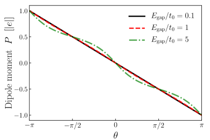
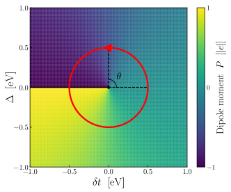
Figure S3: On the left panel, behaviour of the dipole moment per unit cell $P$ with respect to $\theta$ for different values of $E_{\mathrm{gap}}/t_{0}$. As expected, in the small-gap limit ($E_{\mathrm{gap}}\lesssim t_{0}$) we observe the linear behaviour $P\propto-\theta$ predicted in Equation (S49). On the right panel are reported the values of $P$ for each point of the 2D parametric $(\Delta,\delta t)-$space. An adiabatic evolution along a loop containing the origin of the axes (which correspond to a metallic system) pumps out a quantised charge of $-2|e|$.

Numerical calculations

Structural information

For each value of the long-range mixing parameter $c_{\mathrm{LR}}$, a geometric optimisation was performed in order to obtain the equilibrium structures. The unit cell length $a_{0}$ has a very weak dependence on $c_{\mathrm{LR}}$ for all the polymers studied, as shown in Figure S4. Signatures of the second order phase transition in MFPA and PMI are provided by the behaviour of the bond lengths and bond angles, reported in Figure S5. Conversely, the structure of PVDF is not affected by changes in the $c_{\mathrm{LR}}$ parameter, as highlighted in Figure S6.

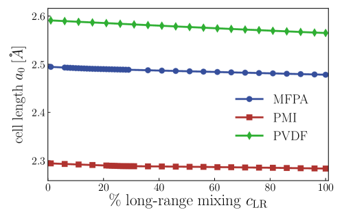
Figure S4: Values of the cell length $a_{0}$ obtained through a cell relaxation for different values of the long-range mixing parameter $c_{\mathrm{LR}}$.

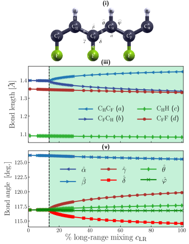
Figure S5: View of the undimerized structure of (i) mono-fluorinated polyacetylene (MFPA) and (ii) polymethineimine (PMI). In (iii) and (iv) for MFPA and PMI, respectively, we report the values of the bond length between the atoms of the unit cell, calculated with different long-range mixing parameter $c_{\mathrm{LR}}$, whereas in (v) and (vi) we report the values of the bond angles for MFPA and PMI, respectively. For MFPA, we use $\mathrm{C_{H}}$ and $\mathrm{C_{F}}$ to label carbon atoms bonded to hydrogen and fluorine, respectively. Bond angles are labeled as follows: $\hat{\alpha}$ and $\hat{\beta}$ denote the $\widehat{\mathrm{C_{F}C_{H}C_{F}}}$ ($\widehat{\mathrm{CNC}}$) and $\widehat{\mathrm{C_{H}C_{F}C_{H}}}$ ($\widehat{\mathrm{NCN}}$) bond angles, while $\hat{\gamma}$ and $\hat{\delta}$ label the $\widehat{\mathrm{C_{H}C_{F}F}}$ ($\widehat{\mathrm{NCH}}$) and $\widehat{\mathrm{FC_{F}C_{H}}}$ ($\widehat{\mathrm{HCN}}$) bond angles. For MFPA only, we also denote by $\hat{\theta}$ and $\hat{\phi}$ the $\widehat{\mathrm{C_{F}C_{H}H}}$ and $\widehat{\mathrm{HC_{H}C_{F}}}$ bond angles. As expected, the phase transition is signalled by the bond-length alternation as well as in the bifurcation of $\hat{\gamma}$ and $\hat{\delta}$ bond angles.

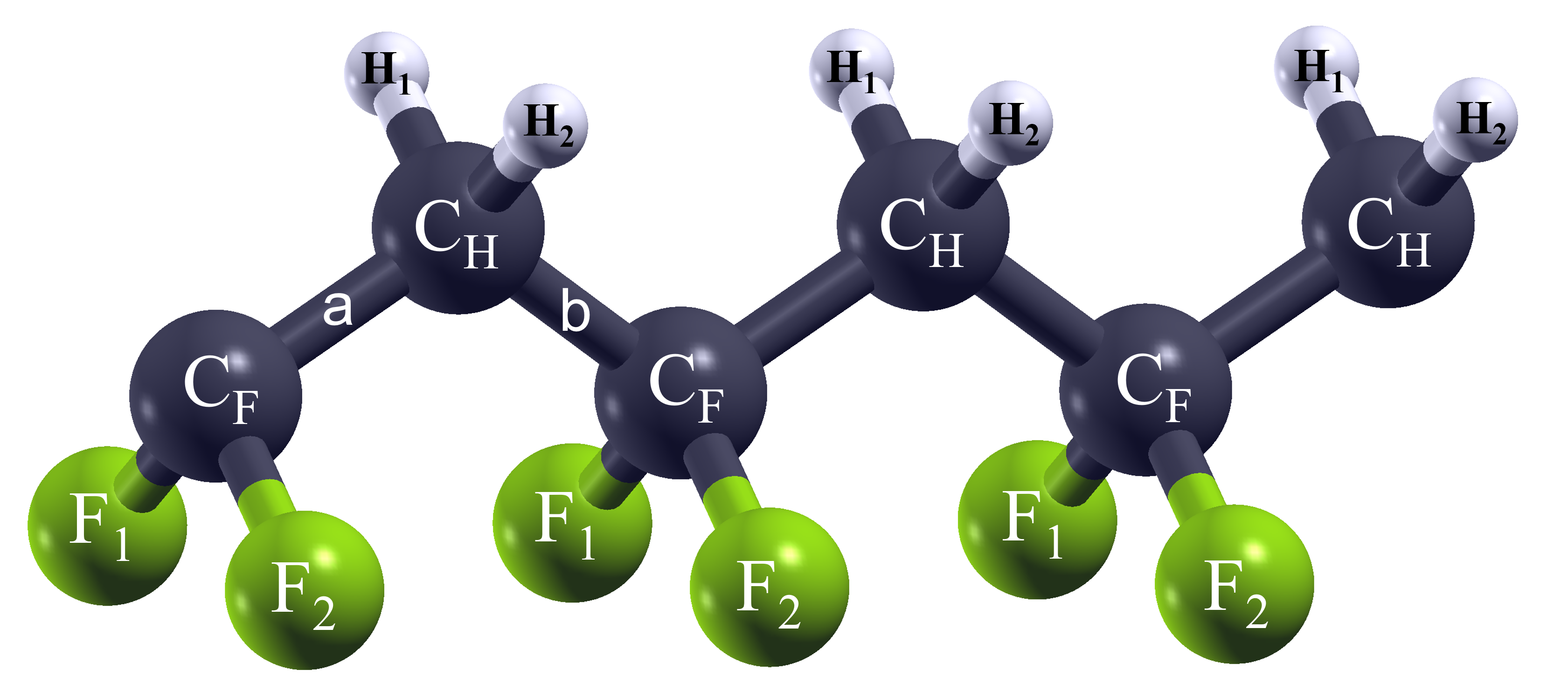
Figure S6: On the left, view of the structure of polyvinylidene fluoride (PVDF). On the right, behaviour of the bond lengths for different values of $c_{\mathrm{LR}}$. As expected, the structure of PVDF depends very weakly on the long-range mixing parameter, this polymer being not conjugated.

Born effective charges of MFPA

Table S1: For three representative values of the long-range mixing parameter $c_{\mathrm{LR}}$ (including the critical value where the chain dimerization occurs), the components of the effective charge tensors for each atom of the unit cell of MFPA are reported. The $Z^{*}_{xx}$ component of the carbon atoms reaches strikingly high values, hint of the anomalous polar response of the $\pi$-orbitals along the backbone chain. The sum rule $Z^{*}_{\mathrm{C_{F}}}+Z^{*}_{\mathrm{C_{H}}}+Z^{*}_{\mathrm{F}}+Z^{*}_{\mathrm{H}}=0$ is also respected.

$\mathbf{c_{\mathrm{\textbf{LR}}}\boldsymbol{=}1\boldsymbol{\%}}$
$Z^{*}_{\mathrm{C_{F}}}$
	$x$	$y$	$z$
$x$	27.830	-0.007	0.000
$y$	-0.013	0.976	0.000
$z$	0.000	0.000	0.168
$Z^{*}_{\mathrm{C_{H}}}$
	$x$	$y$	$z$
$x$	-25.533	-0.001	0.000
$y$	0.013	-0.104	0.000
$z$	0.000	0.000	-0.197
$Z^{*}_{\mathrm{F}}$
	$x$	$y$	$z$
$x$	-2.143	0.010	0.000
$y$	0.001	-0.865	0.000
$z$	0.000	0.000	-0.104
$Z^{*}_{\mathrm{H}}$
	$x$	$y$	$z$
$x$	-0.154	-0.002	0.000
$y$	0.000	-0.007	0.000
$z$	0.000	0.000	0.132

$\boldsymbol{c_{\mathrm{\textbf{LR}}}=13\%\,(\simeq\overline{c}_{\mathrm{\textbf{LR}}})}$
$Z^{*}_{\mathrm{C_{F}}}$
	$x$	$y$	$z$
$x$	30.497	-0.015	0.000
$y$	-0.029	0.991	0.000
$z$	0.000	0.000	0.185
$Z^{*}_{\mathrm{C_{H}}}$
	$x$	$y$	$z$
$x$	-28.090	-0.006	0.000
$y$	0.028	-0.113	0.000
$z$	0.000	0.000	-0.214
$Z^{*}_{\mathrm{F}}$
	$x$	$y$	$z$
$x$	-2.240	0.028	0.000
$y$	0.001	-0.876	0.000
$z$	0.000	0.000	-0.106
$Z^{*}_{\mathrm{H}}$
	$x$	$y$	$z$
$x$	-0.167	-0.008	0.000
$y$	0.000	-0.002	0.000
$z$	0.000	0.000	0.135

$\mathbf{c_{\mathrm{\textbf{LR}}}\boldsymbol{=}100\boldsymbol{\%}}$
$Z^{*}_{\mathrm{C_{F}}}$
	$x$	$y$	$z$
$x$	3.969	-0.901	0.000
$y$	-0.334	1.100	0.000
$z$	0.000	0.000	0.217
$Z^{*}_{\mathrm{C_{H}}}$
	$x$	$y$	$z$
$x$	-3.426	0.145	0.000
$y$	0.316	-0.154	0.000
$z$	0.000	0.000	-0.241
$Z^{*}_{\mathrm{F}}$
	$x$	$y$	$z$
$x$	-0.576	0.088	0.000
$y$	0.021	-0.961	0.000
$z$	0.000	0.000	-0.118
$Z^{*}_{\mathrm{H}}$
	$x$	$y$	$z$
$x$	0.031	-0.124	0.000
$y$	-0.003	0.015	0.000
$z$	0.000	0.000	0.143

Born effective charges of PMI

Table S2: For three representative values of the long-range mixing parameter $c_{\mathrm{LR}}$ (including the critical value where the chain dimerization occurs), the components of the effective charge tensors for each atom of the unit cell of PMI are reported. The $Z^{*}_{xx}$ component of the backbone atoms reaches strikingly high values, hint of the anomalous polar response of the $\pi$-orbitals along the backbone chain. The sum rule $Z^{*}_{\mathrm{C}}+Z^{*}_{\mathrm{N}}+Z^{*}_{\mathrm{H}}=0$ is also respected.

$\mathbf{c_{\mathrm{\textbf{LR}}}\boldsymbol{=}1\boldsymbol{\%}}$
$Z^{*}_{\mathrm{C}}$
	$x$	$y$	$z$
$x$	14.063	0.000	0.000
$y$	-0.005	0.643	0.000
$z$	0.000	0.000	0.168
$Z^{*}_{\mathrm{N}}$
	$x$	$y$	$z$
$x$	-14.059	0.000	0.000
$y$	0.005	-0.427	0.000
$z$	0.000	0.000	-0.273
$Z^{*}_{\mathrm{H}}$
	$x$	$y$	$z$
$x$	-0.004	0.000	0.000
$y$	0.000	-0.216	0.000
$z$	0.000	0.000	0.105

$\boldsymbol{c_{\mathrm{\textbf{LR}}}=25\%\,(\simeq\overline{c}_{\mathrm{\textbf{LR}}})}$
$Z^{*}_{\mathrm{C}}$
	$x$	$y$	$z$
$x$	15.204	0.004	0.000
$y$	-0.012	0.655	0.000
$z$	0.000	0.000	0.186
$Z^{*}_{\mathrm{N}}$
	$x$	$y$	$z$
$x$	-15.217	-0.001	0.000
$y$	0.012	-0.448	0.000
$z$	0.000	0.000	-0.292
$Z^{*}_{\mathrm{H}}$
	$x$	$y$	$z$
$x$	0.013	-0.003	0.000
$y$	0.000	-0.206	0.000
$z$	0.000	0.000	0.106

$\mathbf{c_{\mathrm{\textbf{LR}}}\boldsymbol{=}100\boldsymbol{\%}}$
$Z^{*}_{\mathrm{C}}$
	$x$	$y$	$z$
$x$	5.762	0.166	0.000
$y$	-0.268	0.638	0.000
$z$	0.000	0.000	0.203
$Z^{*}_{\mathrm{N}}$
	$x$	$y$	$z$
$x$	-5.699	0.022	0.000
$y$	0.267	-0.476	0.000
$z$	0.000	0.000	-0.318
$Z^{*}_{\mathrm{H}}$
	$x$	$y$	$z$
$x$	-0.063	-0.188	0.000
$y$	0.001	-0.162	0.000
$z$	0.000	0.000	0.115

Born effective charges of PVDF

Table S3: Components of the effective charge tensors of the atoms of the unit cell of PVDF. For each component, values reported are obtained as average of those computed with different values of $c_{\mathrm{LR}}$, the highest standard deviation being of the order of $10^{-2}$. The very weak dependence of the effective charges of PVDF on $c_{\mathrm{LR}}$ is a direct consequence of the fact that the structure of PVDF does not depend on $c_{\mathrm{LR}}$, as observed in Figure S6. Our results for the Born effective charges of PVDF are overall consistent with previously reported values calculated within the generalized-gradient approximation[50]. The sum rule $Z^{*}_{\mathrm{C_{F}}}+Z^{*}_{\mathrm{C_{H}}}+Z^{*}_{\mathrm{F_{1}}}+Z^{*}_{\mathrm{F_{2}}}+Z^{*}_{\mathrm{H_{1}}}+Z^{*}_{\mathrm{H_{2}}}=0$ is also respected.

$Z^{*}_{\mathrm{C_{H}}}$
	$x$	$y$	$z$
$x$	-0.603	0.000	0.000
$y$	0.000	0.012	0.000
$z$	-0.001	0.001	-0.092
$Z^{*}_{\mathrm{C_{F}}}$
	$x$	$y$	$z$
$x$	1.333	0.000	0.000
$y$	0.000	1.165	0.000
$z$	0.001	0.000	0.955

$Z^{*}_{\mathrm{H_{1}}}$
	$x$	$y$	$z$
$x$	0.069	0.000	0.000
$y$	0.000	0.002	-0.048
$z$	0.000	-0.060	0.034
$Z^{*}_{\mathrm{F_{1}}}$
	$x$	$y$	$z$
$x$	-0.434	0.000	0.000
$y$	-0.002	-0.590	-0.292
$z$	0.000	-0.248	-0.467

$Z^{*}_{\mathrm{H_{2}}}$
	$x$	$y$	$z$
$x$	0.069	0.000	0.000
$y$	0.000	0.003	0.048
$z$	0.000	0.060	0.035
$Z^{*}_{\mathrm{F_{2}}}$
	$x$	$y$	$z$
$x$	-0.434	0.000	0.000
$y$	0.002	-0.592	0.292
$z$	0.000	0.246	-0.465

References

- [1] S Tadigadapa and K Mateti. Piezoelectric mems sensors: state-of-the-art and perspectives. Measurement Science and technology, 20:092001, 2009.
- [2] Joe Briscoe and Steve Dunn. Piezoelectric nanogenerators–a review of nanostructured piezoelectric energy harvesters. Nano Energy, 14:15–29, 2015.
- [3] Don Berlincourt. Piezoelectric crystals and ceramics. In Ultrasonic transducer materials, pages 63–124. Springer, 1971.
- [4] Hans Jaffe. Piezoelectric ceramics. Journal of the American Ceramic Society, 41:494–498, 1958.
- [5] J. Rödel, W. Jo, K. T. P. Seifert, E.-M. Anton, T. Granzow, and D. Damjanovic. Perspective on the development of lead-free piezoceramics. Journal of the American Ceramic Society, 92:1153–1177, 2009.
- [6] Y. Saito, H. Takao, T. Tani, and et al. Lead-free piezoceramics. Nature, 432:84–87, 2009.
- [7] N Setter, D Damjanovic, L Eng, G Fox, Spartak Gevorgian, S Hong, A Kingon, H Kohlstedt, NY Park, GB Stephenson, et al. Ferroelectric thin films: Review of materials, properties, and applications. Journal of applied physics, 100:051606, 2006.
- [8] Andrew J Lovinger. Ferroelectric polymers. Science, 220:1115–1121, 1983.
- [9] Khaled S Ramadan, Dan Sameoto, and Sthephane Evoy. A review of piezoelectric polymers as functional materials for electromechanical transducers. Smart Materials and Structures, 23:033001, 2014.
- [10] Thangavel Vijayakanth, David J. Liptrot, Ehud Gazit, Ramamoorthy Boomishankar, and Chris R. Bowen. Recent advances in organic and organic–inorganic hybrid materials for piezoelectric mechanical energy harvesting. Advanced Functional Materials, 32:2109492, 2022.
- [11] P. Saxena and P. Shukla. A comprehensive review on fundamental properties and applications of poly(vinylidene fluoride) (PVDF). Adv Compos Hybrid Mater, 4:8–26, 2020.
- [12] H. Fu and R. Cohen. Polarization rotation mechanism for ultrahigh electromechanical response in single-crystal piezoelectrics. Nature, 403:281, 2000.
- [13] Z. Kutnjak, J. Petzelt, and R. Blinc. The giant electromechanical response in ferroelectric relaxors as a critical phenomenon. Nature, 441:956, 2006.
- [14] Muhtar Ahart, Maddury Somayazulu, RE Cohen, P Ganesh, Przemyslaw Dera, Ho-kwang Mao, Russell J Hemley, Yang Ren, Peter Liermann, and Zhigang Wu. Origin of morphotropic phase boundaries in ferroelectrics. Nature, 451:545–548, 2008.
- [15] Dragan Damjanovic. A morphotropic phase boundary system based on polarization rotation and polarization extension. Applied Physics Letters, 97:062906, 2010.
- [16] Y. Liu, H. Aziguli, B. Zhang, W. Xu, W. Lu, J. Bernholc, and Wang Q. Ferroelectric polymers exhibiting behaviour reminiscent of a morphotropic phase boundary. Nature, 562:96, 2018.
- [17] Jiseul Park, Yeong-won Lim, Sam Yeon Cho, Myunghwan Byun, Kwi-Il Park, Han Eol Lee, Sang Don Bu, Ki-Tae Lee, Qing Wang, and Chang Kyu Jeong. Ferroelectric polymer nanofibers reminiscent of morphotropic phase boundary behavior for improved piezoelectric energy harvesting. Small, 18:2104472, 2022.
- [18] William Barford. Electronic and optical properties of conjugated polymers. Oxford University Press, 2013.
- [19] Hugo Bronstein, Christian B Nielsen, Bob C Schroeder, and Iain McCulloch. The role of chemical design in the performance of organic semiconductors. Nature Reviews Chemistry, pages 1–12, 2020.
- [20] Shigeki Onoda, Shuichi Murakami, and Naoto Nagaosa. Topological nature of polarization and charge pumping in ferroelectrics. Physical review letters, 93:167602, 2004.
- [21] N. Kirova and S. Brazovskii. Electronic ferroelectricity in carbon based materials. Synthetic Metals, 216:11–22, 2016.
- [22] M.J. Rice and E.J. Mele. Elementary excitations of a linearly conjugated diatomic polymer. Physical Review Letters, 49:1455, 1982.
- [23] Kunihiko Yamauchi and Paolo Barone. Electronic ferroelectricity induced by charge and orbital orderings. Journal of Physics: Condensed Matter, 26:103201, 2014.
- [24] Di Xiao, Ming-Che Chang, and Qian Niu. Berry phase effects on electronic properties. Reviews of modern physics, 82:1959, 2010.
- [25] W. P. Su, J.R. Schrieffer, and A. J. Heeger. Solitons in polyacetylene. Physical review letters, 42:1698, 1979.
- [26] Toshio Masuda. Substituted polyacetylenes. Journal of Polymer Science Part A: Polymer Chemistry, 45:165–180, 2007.
- [27] DJ Thouless. Quantization of particle transport. Physical Review B, 27:6083, 1983.
- [28] Shuta Nakajima, Takafumi Tomita, Shintaro Taie, Tomohiro Ichinose, Hideki Ozawa, Lei Wang, Matthias Troyer, and Yoshiro Takahashi. Topological thouless pumping of ultracold fermions. Nature Physics, 12:296–300, 2016.
- [29] H. Rostami, F. Guinea, M. Polini, and R. Roldán. Piezoelectricity and valley chern number in inhomogeneous hexagonal 2d crystals. npj 2D Mater. Appl., 2:15, 2018.
- [30] Oliviero Bistoni, Paolo Barone, Emmanuele Cappelluti, Lara Benfatto, and Francesco Mauri. Giant effective charges and piezoelectricity in gapped graphene. 2D Materials, 6:045015, 2019.
- [31] B. A. Glavin and S. S. Kubakaddi. Influence of dielectric environment on screening of electron-phonon interaction in quantum well structures. Phys. Rev. B, 74:033312, Jul 2006.
- [32] Maarten L. Van de Put, Gautam Gaddemane, Sanjay Gopalan, and Massimo V. Fischetti. Effects of the dielectric environment on electronic transport in monolayer mos2: Screening and remote phonon scattering. In 2020 International Conference on Simulation of Semiconductor Processes and Devices (SISPAD), pages 281–284, 2020.
- [33] Michele Casula, Matteo Calandra, and Francesco Mauri. Local and nonlocal electron-phonon couplings in k3 picene and the effect of metallic screening. Phys. Rev. B, 86:075445, Aug 2012.
- [34] Thibault Sohier, Matteo Calandra, and Francesco Mauri. Two-dimensional fröhlich interaction in transition-metal dichalcogenide monolayers: Theoretical modeling and first-principles calculations. Phys. Rev. B, 94:085415, Aug 2016.
- [35] Francesco Macheda, Thibault Sohier, Paolo Barone, and Francesco Mauri. Electron-phonon interaction and phonon frequencies in two-dimensional doped semiconductors. Phys. Rev. B, 107:094308, Mar 2023.
- [36] D. M. Basko and I. L. Aleiner. Interplay of coulomb and electron-phonon interactions in graphene. Phys. Rev. B, 77:041409, Jan 2008.
- [37] Tommaso Venanzi, Lorenzo Graziotto, Francesco Macheda, Simone Sotgiu, Taoufiq Ouaj, Elena Stellino, Claudia Fasolato, Paolo Postorino, Vaidotas Mišeikis, Marvin Metzelaars, Paul Kögerler, Bernd Beschoten, Camilla Coletti, Stefano Roddaro, Matteo Calandra, Michele Ortolani, Christoph Stampfer, Francesco Mauri, and Leonetta Baldassarre. Probing enhanced electron-phonon coupling in graphene by infrared resonance raman spectroscopy. Phys. Rev. Lett., 130:256901, Jun 2023.
- [38] Matteo Calandra, Paolo Zoccante, and Francesco Mauri. Universal increase in the superconducting critical temperature of two-dimensional semiconductors at low doping by the electron-electron interaction. Phys. Rev. Lett., 114:077001, Feb 2015.
- [39] Betül Pamuk, Jacopo Baima, Roberto Dovesi, Matteo Calandra, and Francesco Mauri. Spin susceptibility and electron-phonon coupling of two-dimensional materials by range-separated hybrid density functionals: Case study of . Phys. Rev. B, 94:035101, Jul 2016.
- [40] Davide Romanin, Lorenzo Monacelli, Raffaello Bianco, Ion Errea, Francesco Mauri, and Matteo Calandra. Dominant role of quantum anharmonicity in the stability and optical properties of infinite linear acetylenic carbon chains. The Journal of Physical Chemistry Letters, 12:10339–10345, 2021.
- [41] Jonathan Laflamme Janssen, Michel Côté, Steven G. Louie, and Marvin L. Cohen. Electron-phonon coupling in using hybrid functionals. Phys. Rev. B, 81:073106, Feb 2010.
- [42] Leeor Kronik and Stephan Kümmel. Dielectric screening meets optimally tuned density functionals. Advanced Materials, 30:1706560, 2018.
- [43] Sivan Refaely-Abramson, Sahar Sharifzadeh, Manish Jain, Roi Baer, Jeffrey B. Neaton, and Leeor Kronik. Gap renormalization of molecular crystals from density-functional theory. Phys. Rev. B, 88:081204, Aug 2013.
- [44] Daniel Lüftner, Sivan Refaely-Abramson, Michael Pachler, Roland Resel, Michael G. Ramsey, Leeor Kronik, and Peter Puschnig. Experimental and theoretical electronic structure of quinacridone. Phys. Rev. B, 90:075204, Aug 2014.
- [45] Arun K. Manna, Sivan Refaely-Abramson, Anthony M. Reilly, Alexandre Tkatchenko, Jeffrey B. Neaton, and Leeor Kronik. Quantitative prediction of optical absorption in molecular solids from an optimally tuned screened range-separated hybrid functional. Journal of Chemical Theory and Computation, 14:2919–2929, 2018.
- [46] P. Vogl. Microscopic theory of electron-phonon interaction in insulators or semiconductors. Phys. Rev. B, 13:694–704, Jan 1976.
- [47] Francesco Macheda, Paolo Barone, and Francesco Mauri. Electron-phonon interaction and longitudinal-transverse phonon splitting in doped semiconductors. Physical Review Letters, 129:185902, 2022.
- [48] Ph. Ghosez, J.-P. Michenaud, and X. Gonze. Dynamical atomic charges: The case of compounds. Phys. Rev. B, 58:6224–6240, Sep 1998.
- [49] Serge M Nakhmanson, M Buongiorno Nardelli, and Jerry Bernholc. Ab initio studies of polarization and piezoelectricity in vinylidene fluoride and bn-based polymers. Physical review letters, 92:115504, 2004.
- [50] Nicholas J. Ramer and Kimberly A. Stiso. Structure and born effective charge determination for planar-zigzag -poly(vinylidene fluoride) using density-functional theory. Polymer, 46:10431–10436, 2005.
- [51] RD King-Smith and David Vanderbilt. Theory of polarization of crystalline solids. Physical Review B, 47:1651, 1993.
- [52] Raffaele Resta. Manifestations of berry’s phase in molecules and condensed matter. Journal of Physics: Condensed Matter, 12:R107, 2000.
- [53] John P Perdew, Matthias Ernzerhof, and Kieron Burke. Rationale for mixing exact exchange with density functional approximations. The Journal of chemical physics, 105:9982–9985, 1996.
- [54] Roberto Dovesi, Roberto Orlando, Alessandro Erba, Claudio M Zicovich-Wilson, Bartolomeo Civalleri, Silvia Casassa, Lorenzo Maschio, Matteo Ferrabone, Marco De La Pierre, Philippe d’Arco, et al. Crystal14: A program for the ab initio investigation of crystalline solids, 2014.
- [55] Roberto Dovesi, Alessandro Erba, Roberto Orlando, Claudio M Zicovich-Wilson, Bartolomeo Civalleri, Lorenzo Maschio, Michel Rérat, Silvia Casassa, Jacopo Baima, Simone Salustro, et al. Quantum-mechanical condensed matter simulations with crystal. Wiley Interdisciplinary Reviews: Computational Molecular Science, 8:e1360, 2018.
- [56] Daniel Vilela Oliveira, Joachim Laun, Michael F Peintinger, and Thomas Bredow. Bsse-correction scheme for consistent gaussian basis sets of double-and triple-zeta valence with polarization quality for solid-state calculations. Journal of Computational Chemistry, 40:2364–2376, 2019.
- [57] Elon Weintraub, Thomas M Henderson, and Gustavo E Scuseria. Long-range-corrected hybrids based on a new model exchange hole. Journal of Chemical Theory and Computation, 5:754–762, 2009.
- [58] Fabien Pascale, Claudio Marcelo Zicovich-Wilson, F López Gejo, Bartolomeo Civalleri, Roberto Orlando, and Roberto Dovesi. The calculation of the vibrational frequencies of crystalline compounds and its implementation in the crystal code. Journal of computational chemistry, 25:888–897, 2004.
- [59] David Vanderbilt. Berry-phase theory of proper piezoelectric response. Journal of Physics and Chemistry of Solids, 61:147–151, 2000.
- [60] A Erba, Kh E El-Kelany, M Ferrero, Isabelle Baraille, and Michel Rérat. Piezoelectricity of srtio 3: An ab initio description. Physical Review B, 88:035102, 2013.
- [61] Alessandro Erba. The internal-strain tensor of crystals for nuclear-relaxed elastic and piezoelectric constants: on the full exploitation of its symmetry features. Physical Chemistry Chemical Physics, 18:13984–13992, 2016.
- [62] Michael Victor Berry. Quantal phase factors accompanying adiabatic changes. Proceedings of the Royal Society of London. A. Mathematical and Physical Sciences, 392:45–57, 1984.