State-space models are widely used in many applications. In the domain of count data, one such example is the model proposed by Harvey and Fernandes, (1989). Unlike many of its parameter-driven alternatives, this model is observation-driven, leading to closed-form expressions for the predictive density. In this paper, we demonstrate the need to extend the model of Harvey and Fernandes, (1989) by showing that their model is not variance stationary. Our extension can accommodate for a wide range of variance processes that are either increasing, decreasing, or stationary, while keeping the tractability of the original model. Simulation and numerical studies are included to illustrate the performance of our method.

A Classification of Observation-Driven State-Space Count Models for Panel Data

Keywords: dependence, posterior ratemaking, dynamic random effects, conjugate-prior, local-level models, state-space model, experience rating.

JEL Classification: C32; C53

MSC:62M10.

1 Introduction

Time series of counts data are widely used in many areas such as insurance, finance, marketing, economics, etc. According to Cox, (1981), there are two major types of time series models, called observation-driven and parameter-driven, respectively. In the count time series framework, the most popular observation-driven time series models are thinning based models, such as INAR($p$) and INGARCH models; see, e.g., Lu, (2021); Davis et al., (2021) for a review. These models are not state-space based, whereas the best known state-space models include, for instance, Zeger, (1988); Henderson and Shimakura, (2003); Frühwirth-Schnatter and Wagner, (2006); Cui and Lund, (2009); Davis and Wu, (2009); Jung et al., (2011); Jia et al., (2023), to name a few.

Compared to INAR($p$) and INGARCH models, state-space models have several advantages:

• First, it is more convenient to include covariates (i.e., regressors).

• Second, it is more convenient to address missing values, as well as changes of exposures in a state-space framework.

• Third, stationarity (or non-stationary) is more tractable under a state-space framework, and in the case of a stationary process, the marginal distribution is often simple to work out.

These three properties can be essential in applications involving panel (i.e., longitudinal) data. One typical example is car insurance pricing, where the insurer observes, for each year, the values of the covariates, as well as a count response variable representing the annual number of claims. Let us explain the importance of these three properties in more detail.

Allowing for covariates

Most INAR and INARCH (or INGARCH) type models are used without including covariates. The only exceptions we are aware of are Davis et al., (2003) and Agosto et al., (2016). These models directly postulate conditional distributions of the future observations, whose parameters are functions of the current values of the covariates. A drawback of this approach is that past values of the covariates do not enter into the conditional distribution. To see why past covariate values could be important for car insurance pricing, let us assume, for expository purpose, that the covariate $X_{t}$ is univariate, and that given past claim numbers $Y_{t-1},Y_{t-2},\ldots$ and past and current covariate values, the conditional expectation (i.e., the premium) of $Y_{t}$ is increasing in $X_{t}$. In other words, $X_{t}$ measures the underlying risk of the policy. Then, given $Y_{t-1},\ldots$ and $X_{t}$, the premium should be decreasing in past covariate values $X_{t-1},\ldots$, this is because the larger $X_{t-1},\ldots$, the more “efforts” the policyholder made in the past to arrive at the given numbers of claims $Y_{t-1},\ldots$. Because these efforts are statistically likely to continue in the future, the premium should be decreasing in $X_{t-1},\ldots$; we refer to Equation (15) of Dionne and Vanasse, (1989) for an example of a premium function that satisfies this decreasingness constraint.

Accounting for missing values and change of exposure

In car insurance, it is common for the insurance policies to be analyzed by calendar year. Then for each policy, the first observation is usually left truncated (due to policy inceptions during the calendar year), with an exposure equal to only a fraction of a year. Similarly, the last observation could be censored because of early termination of the policy. These differences of exposure can be conveniently handled by multiplying the stochastic Poisson parameter in the state-space model by an offset term being equal to the fraction of the year covered. It is less straightforward to adjust for such changes of exposures under the INAR and the INGARCH framework, respectively.

Analyzing stationarity and stationary distribution

In a longitudinal data context, the likelihood function involves the initial distribution of the observed process. Indeed, for each given individual, the joint probability density function (pdf) of the first $n$ observations can be decomposed as

$$f(Y_{1},Y_{2},\ldots,Y_{T})=f(Y_{1})f(Y_{2}|Y_{1})f(Y_{3}|Y_{1},Y_{2})\cdots f(Y_{T}|Y_{T-1},\ldots,Y_{1}),$$

where the first term $f(Y_{1})$ is the marginal pdf of the first response $Y_{1}$. In observation-driven count models such as INAR($p$) and IN(G)ARCH, the subsequent terms corresponding to the conditional distributions are usually more tractable, but the first term can be rather cumbersome. This first term can be omitted, only if the time series length $T$ is very large. When $T$ is small, however, its omission induces a bias.

In state-space models, on the other hand, the term $F(Y_{1})$ is often tractable, since $Y_{1}$ is the output of a latent variable $\Theta_{1}$, whose distribution is usually chosen simple. For instance, in many parameter-driven models, the latent process $(\Theta_{t})$ is assumed stationary and ergodic, following a Gaussian AR(1) or an autoregressive gamma process. Then, the marginal distribution of $\Theta_{1}$ is simple.

Despite the three aforementioned advantages of state-space count models, many parameter-driven state-space models often suffer from a much higher computational burden since the latent process $(\Theta_{t})$ has to be integrated out, which leads to a $T$-dimensional integral that may be approximated via Monte Carlo simulation; see, e.g., Chan and Ledolter, (1995), Frühwirth-Schnatter and Wagner, (2006). This makes their implementation challenging, especially in a longitudinal data context with a large cross-sectional dimension; see, e.g., Lu, (2018) for a discussion in the context of insurance pricing.

Harvey and Fernandes, (1989)’s model (henceforth HF model) is one of the rare examples of observation-driven state-space models, that enjoys the three properties above, while still being tractable. More precisely, in contrast to its parameter-driven counterparts, the dynamics of this latter model is not exogenous, but endogenous, in the sense that the dynamics depends not only on the past values of the state variable, but also on the past values of the observed responses

$$\Theta_{t+1}|(\Theta_{1:t},Y_{1:t})~{}=~{}\Theta_{t+1}|(\Theta_{t},Y_{1:t}).$$ (1)

where $Y_{1:t}=(Y_{1},\ldots,Y_{t})$ and $\Theta_{1:t}=(\Theta_{1},\ldots,\Theta_{t})$ denote the processes of the past claim observations, $(Y_{t})$, and the latent risk factors up to time $t$, $(\Theta_{t})$, respectively. The tractability of the predictive distribution arises from the Poisson-gamma conjugacy, by assuming that the conditional distributional on the right hand side of (1) is a gamma distribution, while the conditional distribution in the measurement equation of $Y_{t}$, given $\Theta_{t}$, is assumed to be Poisson. This model can be regarded as the count valued analog of a Bayesian state-space model that relies on conjugate priors, such as Smith and Miller, (1986) and Shephard, (1994) for real-valued univariate processes, and Uhlig, (1997) for real-valued multivariate processes. It has recently been applied by Ahn et al., (2023) in an insurance pricing context.

In this paper we start by explaining that in the HF model, the state variable follows a (multiplicative) random walk, and it has a non-stationary (increasing) variance process. This explosion-in-variance property might not be appropriate in many applications. Therefore, we extend the HF model to accommodate for various other types of variance dynamics. In particular, we classify the extended class of observation-driven state-space models into several groups:

• The original HF model, which has an explosive (non-stationary) dynamics with increasing variance ${\mathrm{V}ar}\left(\Theta_{t}\right)$ with time $t\geq 1$.

• The second class corresponds to the case where, when $t$ goes to infinity, the latent process $(\Theta_{t})$ degenerates to a constant and, hence, the uncertainty related to the non-observability of the latent factor $\Theta_{t}$ asymptotically vanishes.

• In the third class, the latent process $(\Theta_{t})$ considered in (1) has a variance process that is bounded (from zero and infinity). This class includes the special cases where the variance process is time-invariant or converging. This third case is probably the most realistic situation for car insurance pricing, where we learn the unobservable risk factors of the insurance policyholders over time, but there always remains some uncertainty.

The models in these three classes differ in terms of their (variance) stationarity properties, but they all enjoy the three aforementioned properties in terms of covariates, change of exposure, and stationary distributions.

Our paper also contributes to the forecasting literature on exponential moving average or exponential smoothing; see Hyndman et al., (2008), Chapter 16, for a review of such methods for count data. This literature has traditionally focused on models with increasing variance, such as the HF model, which gives rise to an exponentially weighted moving average (EWMA) predictor. In this paper we show that many count process models with bounded variance also allow for EWMA predictors, hence, broadening the scope of exponential smoothing methods.

The rest of the paper is organized as follows. Section 2 extends the HF model, by allowing some of the parameters of the HF model to be time-varying. Section 3 discusses various specifications of this extended HF family, and it classifies them into different classes according to their stationarity (or non-stationarity) behavior, see Table 1, below. Section 4 illustrates the difference of their long-term dynamics through simulations. Section 5 compares these models using a real insurance dataset. Section 6 concludes. The mathematical proofs are provided in the appendix.

2 The extended HF model

Throughout this paper, we use the following notation.

• ${\rm Gamma}(\alpha,\beta)$: gamma distribution with shape parameter $\alpha>0$ and rate parameter $\beta>0$. It has mean $\alpha/\beta$ and variance $\alpha/\beta^{2}$. By convention, we use ${\rm Gamma}(0,\beta)$ to denote a constant zero.

• ${\rm Beta}(\alpha,\beta)$: beta distribution on $(0,1)$ with mean $\frac{\alpha}{\alpha+\beta}$ and variance $\frac{\alpha\beta}{(\alpha+\beta)^{2}(\alpha+\beta+1)}$. By convention, we use ${\rm Beta}(\alpha,0)$ to denote a constant one.

• ${\rm Pois}(\lambda)$: Poisson distribution with mean $\lambda>0$.

• ${\rm NB}(\lambda,\Gamma)$: negative binomial (NB) distribution with mean $\lambda$ and variance $\lambda+\lambda^{2}/\Gamma.$

We recall the usual Poisson-gamma relationship. If $Y$ is Poisson, given $\Theta$, with mean $\Theta$, and $\Theta$ follows a gamma prior distribution, then the posterior distribution of $\Theta$, given $Y$, is still a gamma distribution, and the marginal distribution of $Y$ is a NB distribution.

2.1 The model

We provide an observation-driven state-space model with constant mean, which generalizes the HF model.

Model 1.

Given exogenous processes $\left(\lambda_{t}\right)_{t\geq 1},\ \left(q_{t}^{*}\right)_{t\geq 1}\ \hbox{and}\ \left(q_{t}^{**}\right)_{t\geq 1}$ satisfying for $t\geq 1$

$$0\leq q_{t}^{*}\leq q_{t}^{**}\leq 1\quad\text{ and }\quad q_{t}^{**},\lambda_{t}>0,$$ (2)

the response variables $(Y_{t})_{t\geq 1}$ and the state-space variables (random effects) $(\Theta_{t})_{t\geq 1}$ satisfy:

1. The conditional distribution of $Y_{t}$, given the state variable and past observations $Y_{1:(t-1)}$, is Poisson

   $$Y_{t}|\left(Y_{1:(t-1)},\Theta_{1:t}\right)\sim{\rm Pois}\left(\lambda_{t}\Theta_{t}\right),\qquad\text{ for $t\geq 1$}.$$ (3)

2. At time $t=1$, $\Theta_{1}$ is gamma distributed as

   $$\Theta_{1}\sim{\rm Gamma}\left(\alpha_{1|0},\beta_{1|0}\right),$$ (4)

   where, for identification purposes, we assume equal deterministic parameters $\alpha_{1|0}=\beta_{1|0}>0$, so that ${\mathbb{E}}\left[\Theta_{1}\right]=1$.

3. At time $t\geq 1$, the filtering distribution of $\Theta_{t}$, given past observations $Y_{1:t}$, is gamma

   $$\Theta_{t}|Y_{1:t}\sim{\rm Gamma}\left(\alpha_{t},\beta_{t}\right),$$ (5)

   where $\alpha_{t}>0$ and $\beta_{t}>0$ are deterministic functions of $Y_{1:t}$ and $\lambda_{1:t}$ up to time $t$

   $$\alpha_{t}=\begin{cases}\alpha_{t|t-1}+Y_{t},&\hbox{if $Y_{t}$ is observed};\\ \alpha_{t|t-1},&\hbox{otherwise};\end{cases}$$ (6)

   and

   $$\beta_{t}=\begin{cases}\beta_{t|t-1}+\lambda_{t},&\hbox{if $Y_{t}$ is observed};\\ \beta_{t|t-1},&\hbox{otherwise}.\end{cases}$$ (7)

4. At time $t+1\geq 1$, the predictive distribution of $\Theta_{t+1}$, given $Y_{1:t}$, is gamma with

   $$\Theta_{t+1}|Y_{1:t}\sim{\rm Gamma}\left(\alpha_{t+1|t},\beta_{t+1|t}\right),$$ (8)

   with for $t\geq 1$

   $$\alpha_{t+1|t} = q_{t}^{*}\alpha_{t}+\left(q_{t}^{**}-q_{t}^{*}\right)\beta_{t},$$

   $$\beta_{t+1|t} = q_{t}^{**}\beta_{t}.$$

Definitions (6) and (7) follow from Bayes’ rule, and $\alpha_{t}>0$ and $\beta_{t}>0$ are deterministic functions of the past observations $Y_{1:t}$, up to time $t$, and of $\lambda_{1:t}$, the latter allows to integrate time-varying covariates. From this, we deduce that the conditional distribution of $Y_{t}$, given $Y_{1:(t-1)}$, is negative binomial with

$$Y_{t}\,|\,Y_{1:(t-1)}\sim{\rm NB}\left(\lambda_{t}\,\frac{\alpha_{t|t-1}}{\beta_{t|t-1}},\,\alpha_{t|t-1}\right),$$ (9)

where the conditional probability mass function is given as follows

$$f\left(\left.Y_{t}\right|Y_{1:(t-1)}\right)=\frac{\Gamma\left(Y_{t}+\alpha_{t|t-1}\right)}{Y_{t}!\,\Gamma\left(\alpha_{t|t-1}\right)}\left(\frac{\lambda_{t}}{\lambda_{t}+\beta_{t|t-1}}\right)^{Y_{t}}\left(\frac{\beta_{t|t-1}}{\lambda_{t}+\beta_{t|t-1}}\right)^{\alpha_{t|t-1}}.$$ (10)

In particular, the predictive mean is

$$\mathbb{E}[Y_{t}|Y_{1:(t-1)}] =\lambda_{t}\,\frac{\alpha_{t|t-1}}{\beta_{t|t-1}}.$$ (11)

2.2 Stochastic representation of the observation-driven property

Model 1 defines the conditional distributions of the latent variable $\Theta_{t}$, given the past (or past and current) observations. However, it does not provide a state equation directly linking $\Theta_{t}$ with $\Theta_{t+1}$. To work out this state equation, we first recall the following lemma.

Lemma 1 (Lukacs, (1955)).

Consider two independent random variables

$$\Theta \sim{\rm Gamma}(\alpha,\beta),$$ (12)

$$B \sim{\rm Beta}\left(q^{*}\alpha,(1-q^{*})\alpha\right),$$

where $\alpha>0,\beta>0$, and $q^{*}\in(0,1]$ are given constants. Then, their product

$$\Theta B\sim{\rm Gamma}(q^{*}\alpha,\beta).$$

As a consequence, if $\eta$ is independent of $\Theta$ and $B$, and $\eta\sim{\rm Gamma}((q^{**}-q^{*})\beta,q^{**}\beta)$ with constant $q^{**}$ such that $q^{**}\geq q^{*}$, then we have:

$$\frac{\Theta B}{q^{**}}+\eta\sim{\rm Gamma}\left(q^{*}\alpha+\left(q^{**}-q^{*}\right)\beta,q^{**}\beta\right).$$ (13)

Formula (13) implies the following stochastic representation of the latent process $(\Theta_{t})_{t\geq 1}$:

$$\Theta_{t+1}=\frac{\Theta_{t}B_{t+1}}{q_{t}^{**}}+\eta_{t+1},$$ (14)

where

$$B_{t+1}\,|\,(Y_{1:t},\Theta_{1:t})\sim{\rm Beta}(q_{t}^{*}\alpha_{t},(1-q_{t}^{*})\alpha_{t}),$$

and

$$\eta_{t+1}\,|\,(Y_{1:t},\Theta_{1:t})\sim{\rm Gamma}((q_{t}^{**}-q_{t}^{*})\beta_{t},q_{t}^{**}\beta_{t}).$$

Moreover, $B_{t+1}$ and $\eta_{t+1}$ are conditionally independent, given $Y_{1:t}$ and $\Theta_{1:t}$. The observation-driven nature of the evolution in (1) is evident from the evolution mechanism in (13)-(14), and this justifies the choice of (8) by an explicit example.

2.3 Link with other time series models

Link with random coefficient AR(1) processes

We remark that conditional on the information up to time $t$ in (14), we have

$${\mathbb{E}}\left[\frac{B_{t+1}}{q_{t}^{**}}\,\bigg{|}\,\Theta_{1:t},Y_{1:t}\right]=\frac{q_{t}^{*}}{q_{t}^{**}}\leq 1.$$

Thus, the process $(\Theta_{t})$ can be compared with a (random coefficient) auto-regressive process, see, e.g., Joe, (1996) and Jørgensen and Song, (1998), in which the first term in (14) describes a (stochastic) thinning of the previous state $\Theta_{t}$, and $\eta_{t+1}$ adds new noise to the update. Our specification of $(\Theta_{t})$ differs from this random coefficient literature by the fact that we consider an endogenous, i.e., observation-driven dynamics of $(\Theta_{t})$.

Link with Kalman filters

It is well known in a linear Gaussian state-space model that all the conditional/filtering/predictive distributions are Gaussian; see Durbin and Koopman, (2012), Chapter 4. This result is based on the Gaussian-Gaussian conjugacy, as well as the closure of the Gaussian distribution to convolution and scaling. Because our model is based on the Poisson-gamma conjugacy, as well as the closure of the gamma distribution to scaling and convolution, it can be viewed as a count variable analogue of the Kalman filter. More generally, state-space models based on other conjugate priors have been proposed by Smith and Miller, (1986), Shephard, (1994), and Uhlig, (1997), to name but a few.

3 A classification according to the behavior of the variance process

In this section, we show that Model 1 can allow for various forms of variance processes, e.g., of increasing, decreasing, constant or stationary type.

3.1 The static shared random effect model

The model with shared (or static) random effect assumes that given a time-invariant latent variable $\Theta_{t}\equiv\Theta$, a.s., for all $t\geq 1$, and with $\Theta$ following a $\text{Gamma}(\beta_{1|0},\beta_{1|0})$ distribution, the counts $Y_{t}$ are conditionally independent with a $\text{Pois}(\lambda_{t}\Theta)$ distribution. For $\lambda_{t}\equiv\lambda>0$, this is a special case of the Bühlmann and Straub, (1970) credibility model.

This is a static shared random effect model is obtained from Model 1 by setting

$$q_{t}^{*}=q_{t}^{**}=1\quad\Longleftrightarrow\quad B_{t+1}\equiv 1,\ \eta_{t+1}\equiv 0.$$ (15)

3.2 HF model: A model with increasing variance

To analyze more sophisticated cases, let us first investigate some properties of Model 1 concerning the first and second order moments of the processes.

Lemma 2.

In Model 1 we have the following moment behaviors for $t\geq 1$

1. ${\mathbb{E}}\left[\alpha_{t}\right]=\beta_{t}$, ${\mathbb{E}}\left[\Theta_{t}\right]=1$ and ${\mathbb{E}}\left[Y_{t}\right]=\lambda_{t}$.

2. ${\mathbb{E}}\left[{\mathrm{V}ar}\left(\Theta_{t}\,|\,Y_{1:t}\right)\right]=\frac{1}{\beta_{t}}$.

3. ${\mathbb{E}}\left[{\mathrm{V}ar}\left(\Theta_{t+1}\,|\,Y_{1:t}\right)\right]=\frac{1}{q_{t}^{**}}\frac{1}{\beta_{t}}$.

4. ${\mathrm{V}ar}\left({\mathbb{E}}\left[\Theta_{t+1}\,|\,Y_{1:t}\right]\right)=\left(\frac{q_{t}^{*}}{q_{t}^{**}}\right)^{2}{\mathrm{V}ar}\left({\mathbb{E}}\left[\Theta_{t}\,|\,Y_{1:t}\right]\right)$.

Proof.

See A.1. ∎

Property $i)$ says that process $(\Theta_{t})$ is mean-stationary. Properties $iii)$ and $iv)$ allow to analyze the variance behavior of $(\Theta_{t})$. Indeed, by the total variance decomposition formula, we get

$${\mathrm{V}ar}\left(\Theta_{t+1}\right) ={\mathbb{E}}\left[{\mathrm{V}ar}\left(\Theta_{t+1}\,|\,Y_{1:t}\right)\right]+{\mathrm{V}ar}\left({\mathbb{E}}\left[\Theta_{t+1}\,|\,Y_{1:t}\right]\right)$$ (16)

$$=\frac{1}{q_{t}^{**}}\frac{1}{\beta_{t}}+\left(\frac{q_{t}^{*}}{q_{t}^{**}}\right)^{2}{\mathrm{V}ar}\left({\mathbb{E}}\left[\Theta_{t}\,|\,Y_{1:t}\right]\right).$$

On the other hand, by using the total variance decomposition formula again, we have

$${\mathrm{V}ar}\left(\Theta_{t}\right) ={\mathbb{E}}\left[{\mathrm{V}ar}\left(\Theta_{t}\,|\,Y_{1:t}\right)\right]+{\mathrm{V}ar}\left({\mathbb{E}}\left[\Theta_{t}\,|\,Y_{1:t}\right]\right)$$

$$=\frac{1}{\beta_{t}}+{\mathrm{V}ar}\left({\mathbb{E}}\left[\Theta_{t}\,|\,Y_{1:t}\right]\right).$$ (17)

Let us now compare equations (16) and (3.2). Because $\frac{1}{q_{t}^{**}}\geq 1$ the first term in (16) is larger than the first one of (3.2). Similarly, because $\left(\frac{q_{t}^{*}}{q_{t}^{**}}\right)^{2}\leq 1$, the second term in (16) is smaller than the second one of (3.2). As a result, the variance process $({\mathrm{V}ar}\left(\Theta_{t}\right))$ in our model is not necessarily monotone. Throughout the rest of this section, we will discuss cases in which this sequence of variances $({\mathrm{V}ar}\left(\Theta_{t}\right))$ is either increasing, time-varying, or decreasing.

In this subsection we start by describing an increasing case. The HF model, Harvey and Fernandes, (1989), is obtained from Model 1 under the extra constraints for $t\geq 1$

$$q_{t}^{*}=q_{t}^{**}=q~{}\in~{}(0,1).$$ (18)

Harvey and Fernandes, (1989)’s original formulation is without covariates, Gamerman et al., (2013) extend their model by introducing time-varying exogenous covariates $(\lambda_{t})$.

In this model, the stochastic representation (14) becomes

$$\Theta_{t+1}=\frac{\Theta_{t}B_{t+1}}{q},$$ (19)

which implies that ${\mathrm{E}}\left[\Theta_{t+1}|Y_{1:t}\right]=\Theta_{t}$. In other words, $(\Theta_{t})$ is a martingale with respect to the filtration generated by $(Y_{1:t})$.

The following lemma shows that under some conditions, this martingale has an explosive variance behavior.

Lemma 3 (Explosive variance in the HF model).

Under the HF Model, if the exogenous process $(\lambda_{t})$ is bounded both both above and below across time $t\geq 1$, then $({\mathrm{V}ar}\left(\Theta_{t}\right))$ and $({\mathrm{V}ar}\left(Y_{t}\right))$ increase to infinity when $t$ goes to infinity.

Proof.

See A.2. ∎

One advantage of the HF model is that under this model, the predictive mean (11) is an exponentially weighted moving average (EWMA) of past observations. The literature on exponential moving average forecasting of counts has traditionally focused on non-stationary models only; see, e.g., Hyndman et al., (2008), Chapter 17. It is seen in the next subsection, however, that it is not the only possible specification leading to EWMA predictors.

3.3 A model with converging variance

In this subsection, we discuss a special case of Model 1 which is asymptotically strongly stationary. By strongly stationarity, we mean that the conditional distribution of $Y_{t+h}$, given $Y_{t}$, converges to a non-degenerate distribution. In other words, in the long run, the process $(Y_{t})$ evolves in a “steady state”, i.e., an “equilibrium”. This implies, in particular, that the variance and mean of the process converge to positive constants. Note also that stationarity does not mean “time-invariant”. Indeed, for large time horizons $h$, the variance of $Y_{t+h}$ converges to a positive constant.

Specifically, we assume, in Model 1, that $q_{t}^{*},q_{t}^{**}$ and $\lambda_{t}$ are all time-invariant for $t\geq 1$

$$q_{t}^{*}=pq,\qquad q_{t}^{**}=q,$$ (20)

for $p,q\in(0,1)$, and

$$\lambda_{t}=\lambda.$$ (21)

Then, we have for $t\geq 1$

$$\alpha_{t} =\alpha_{t|t-1}+Y_{t}=pq\alpha_{t-1}+q\left(1-p\right)\beta_{t-1}+Y_{t},$$ (22)

$$\beta_{t} =\beta_{t|t-1}+\lambda_{t}=q\beta_{t-1}+\lambda_{t},$$

where the second identities need $t\geq 2$. Because our model has as predictive distribution a NB distribution, with the number of trial parameter satisfying a linear recursion, this model coincides with the NB-INGARCH(1,1) model, see Gonçalves et al., (2015), who established its stationarity.

Lemma 4 (Gonçalves et al., (2015)).

If in Model 1 the parameters satisfy (20) and (21), then the process $(Y_{t})$ is asymptotically strongly stationary. In particular, $\left({\mathrm{V}ar}\left(\Theta_{t}\right)\right)$ and $\left({\mathrm{V}ar}\left(Y_{t}\right)\right)$ converge.

Under assumptions (20) and (21), the predictive mean (11) is once again an EWMA of the past observations. In other words, it is an extension of the standard EWMA forecasting literature; see Hyndman et al., (2008).

Remark 1.

There are also other stationary count process models allowing for EWMA predictive mean formulas, such as the INGARCH(1,1), see Ferland et al., (2006), or the NB-INGARCH, see Zhu, (2011). These other models, however, do not admit a state-space representation and, therefore, do not possess the three properties mentioned in the introduction. In other words, among all the stationary count models with an EWMA predictive mean, the model of Gonçalves et al., (2015) has the advantage of having a state-space representation.

3.4 A model with decreasing variance

In this subsection, we consider the special case of Model 1 with the constraint for $t\geq 1$

$$q_{t}^{*}=p~{}\in[0,1)\quad\hbox{and}\quad q_{t}^{**}=1.$$ (23)

This implies for $t\geq 2$, see (22),

$$\alpha_{t}=p\alpha_{t-1}+(1-p)\beta_{t-1}+Y_{t}\quad\hbox{and}\quad\beta_{t}=\beta_{t-1}+\lambda_{t}.$$

If $(\lambda_{t})$ is bounded from below, then both processes $(\beta_{t})$ and $(\alpha_{t})$ go to infinity when $t$ increases to infinity.

Let us study the variance of this process. By comparing (16) and (3.2) with the condition in (23), we get

$${\mathrm{V}ar}\left(\Theta_{t+1}\right)-{\mathrm{V}ar}\left(\Theta_{t}\right)=\left({p}^{2}-1\right){\mathrm{V}ar}\left({\mathbb{E}}\left[\Theta_{t}\,|\,Y_{1:t}\right]\right)=\left({p}^{2}-1\right){\mathrm{V}ar}\left(\frac{\alpha_{t}}{\beta_{t}}\right)<0.$$ (24)

Thus, the latent process $(\Theta_{t})$, and hence $(Y_{t})$, have both a decreasing variance (for the latter it is sufficient to assume that $(\lambda_{t})$ is bounded). Moreover, we have the following stronger result.

Lemma 5.

Under Model 1 and constraint (23), if the exogenous process $(\lambda_{t})$ is bounded both from below and above by positive constants, then $({\mathrm{V}ar}\left(\Theta_{t}\right))$ converges to zero, when $t$ goes to infinity, and $({\mathrm{V}ar}\left(Y_{t}\right))$ converges to $\lambda$, under the additional assumption (21).

Proof.

See A.3. ∎

3.5 A model with constant variance

In this subsection, we discuss a special case of Model 1 for which the variance is a constant. Note that the model in Gonçalves et al., (2015), which is the model in Section 3.3, requires $(\lambda_{t})$ to be time-invariant (21), which might be too restrictive for insurance applications. Moreover, the variance is not time-invariant in Lemma 4, but it only converges to a constant at infinity. In the following, we look at another type of stationarity property, by looking only at the variance of the process $(\Theta_{t})$. However, instead of requiring the variance to converge to a constant when time $t$ goes to infinity, we request it to remain constant for any $t$, that is, for $t\geq 1$

$$1={\mathbb{E}}\left[\Theta_{t}\right]\quad\hbox{and}\quad\frac{1}{\beta_{1|0}}={\mathrm{V}ar}\left(\Theta_{t}\right).$$ (25)

This will in turn allow us to relax the time-invariance assumption on $(\lambda_{t})$. More precisely, by comparing (16) and (3.2), we get immediately the following result.

Lemma 6.

In Model 1, the variance process $({\mathrm{V}ar}\left(\Theta_{t}\right))$ is constant, if and only if $q^{*}_{t}$ and $q^{**}_{t}$ satisfy the following equation for all $t\geq 1$

$$\frac{1}{q^{**}_{t}}\frac{1}{\beta_{t}}+\left(\frac{q^{*}_{t}}{q^{**}_{t}}\right)^{2}\left(\frac{1}{\beta_{1|0}}-\frac{1}{\beta_{t}}\right)=\frac{1}{\beta_{1|0}}.$$ (26)

Thus, there are infinitely many possible combinations of $q^{*}_{t}$ and $q^{**}_{t}$ in order for ${\mathrm{V}ar}\left(\Theta_{t}\right)$ to remain constant. Among such choices, motivated by the conditional linear auto-regressive structure (CLAR(1)) in Grunwald et al., (2000), we may assume the following updating rule

$${\mathbb{E}}\left[\Theta_{t+1}\,|\,Y_{1:t}\right]=p{\mathbb{E}}\left[\Theta_{t}\,|\,Y_{1:t}\right]+1-p,$$ (27)

for some $p\in(0,1)$, which is equivalent to the condition

$$\frac{q^{*}_{t}}{q^{**}_{t}}=p.$$ (28)

Then, under this additional assumption (27), requirement (26) becomes for $t\geq 1$

$$q_{t}^{**}=\frac{\beta_{1|0}}{p^{2}\beta_{1|0}+\left(1-p^{2}\right)\beta_{t}},$$ (29)

which can be calculated recursively from $\beta_{t}=q^{**}_{t-1}\beta_{t-1}+\lambda_{t}$, $t\geq 2$, with initialization $\beta_{1}=\beta_{1|0}+\lambda_{1}$.

3.6 A model with bounded variance

For some applications, the assumption of a time-invariant $(\lambda_{t})$ imposed in the previous subsection might be too restrictive. In this subsection, we relax this assumption, and consider a model satisfying (20) only, but not (21). Then, we get the following result.

Lemma 7.

If in Model 1, (20) is satisfied, and if the process $(\lambda_{t})$ is bounded from both above and below by positive constants, then the variance process $({\mathrm{V}ar}\left(Y_{t}\right))$ is bounded from above.

Proof.

See A.4. ∎

3.7 A typology of models according to the variance process

To summarize, the following table lists all the different models considered in this section.

Model	Condition
Shared random effect	$q_{t}^{*}=q_{t}^{**}=1$
HF model with increasing (explosive) variance	$q_{t}^{*}=q_{t}^{**}=q$, $(\lambda_{t})$ bounded
Decreasing variance	$q_{t}^{*}=p,\ q_{t}^{**}=1$, $(\lambda_{t})$ bounded
Converging variance	$q_{t}^{*}=pq,\ q_{t}^{**}=q,\ \lambda_{t}=\lambda$
Bounded variance	$q_{t}^{*}=pq,\ q_{t}^{**}=q$, $(\lambda_{t})$ bounded
Constant variance	Eq. (26)

Table 1: Typology of various special cases of Model 1 according to the long-run behavior of the variance process. All the constants $p$ and $q$ lie strictly between 0 and 1 in this table. By “$(\lambda_{t})$ bounded”, we mean that it is both upper and lower bounded by positive constants.

Because of Equation (11), the models with a constant $q_{t}^{*}$ in this table yield a prediction of $Y_{t+1}$ as a exponential moving average of past observations $Y_{1},\ldots,Y_{t}$. In this regard, Model 1 broadens the scope of exponential smoothing based forecasting methods. Indeed, when it comes to count data, their focus was predominantly on the HF model, specifically in the context of count data; see Hyndman et al., (2008), Chapter 16.

4 Numerical illustration

In this section, we simulate trajectories of the various examples considered in Section 3, and we illustrate the differences in long-term behavior between them. Throughout all examples, we set $\alpha_{1|0}=\beta_{1|0}=3$, and we let $\lambda_{t}=1$ to simulate 5,000 independent trajectories of $(\Theta_{t})$ for $t=1,\ldots,T=50$, under each of the following specifications on the dynamics of $(\Theta_{t})$:

• Increasing variance of $(\Theta_{t})$ (2nd row of Table 1): $q_{t}^{*}=q_{t}^{**}=0.8$,

• Decreasing variance of $(\Theta_{t})$ (3rd row of Table 1): $q_{t}^{*}=0.8,\ q_{t}^{**}=1$,

• Converging variance of $(\Theta_{t})$ (4th row of Table 1): $q_{t}^{*}=0.8,\ q_{t}^{**}=0.9$,

• Constant variance of $(\Theta_{t})$ (6th row of Table 1): $q_{t}^{*}=0.9q_{t}^{**},\ q_{t}^{**}=\frac{\alpha_{0}}{\alpha_{0}\cdot 0.9^{2}+(1-0.9^{2})\beta_{t}}=\frac{3}{2.43+0.19\beta_{t}}$.

4.1 Long-run behavior of $(\Theta_{t})$

For each of the four models above, we display, in Figure 1, four independent paths over $T=50$ time periods. We observe in the northwest panel that the magnitude of the variation of $(\Theta_{t})$ becomes bigger over time, reflecting an increasing variance process. Moreover, the trajectories are highly persistent, which echos the martingale property (19) in the HF model. In the northeast panel, all trajectories of $(\Theta_{t})$ tend to vary less and less over time, which is consistent with the decreasing variance specification. Moreover, all the trajectories fluctuate around one positive value, which is expected because of the constant mean property of the process. In the model with constant variance, it is observed that the fluctuation level of $(\Theta_{t})$ is stable over time compared to the other scenarios. Lastly, it is shown that the fluctuation level of $(\Theta_{t})$ in the converging variance case is between the fluctuation levels in the constant and decreasing cases.

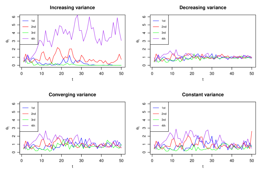
Figure 1: Four independent trajectories of $(\Theta_{t})$ under each of the four specifications. Northwest panel: the model with increasing variance. Northeast panel: the model with decreasing variance. Southwest panel: the model with converging variance. Southeast panel: the model with constant variance.

4.2 Variance of $(\Theta_{t})$

For each of the above four models, we plot the empirical density plots of $\Theta_{t}$ at different times $t=1,5,20,50$, where each time series $(\Theta_{t})$ is simulated 5,000 times. From Figure 2 we observe the following:

• In the HF model with increasing variance, the distribution of $\Theta_{50}$ has both a thicker right tail, and a much higher peak near zero compared to the distributions of $\Theta_{1}$ and $\Theta_{5}$. This reflects the increasing variance of $(\Theta_{t})$ over time under a constant mean, as shown in Figure 2.

• On the other hand, in the model with decreasing variance, the distribution of $\Theta_{50}$ is much more concentrated around the mean value 1 compared to those of $\Theta_{1}$ and $\Theta_{5}$, as the variance of $(\Theta_{t})$ decreases over time.

• In the model with converging variance, we observe that the distribution of $\Theta_{t}$ becomes more concentrated as $t$ increases. Moreover, the distribution of $\Theta_{50}$ is significantly different from, say, $\Theta_{20}$.

• In the model with constant variance, the distributions of $\Theta_{1}$, $\Theta_{5}$, $\Theta_{20}$, and $\Theta_{50}$ are quite close, which reflects the fact they have the same mean and variance.

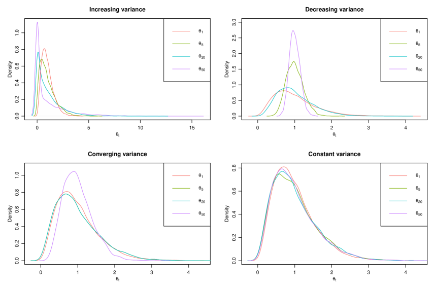
Figure 2: Empirical density of $\Theta_{t}$ under each of the four scenarios at times $t=1,5,20,50$

5 Real data analysis

We use the LGPIF (Local Government Property Insurance Fund) data from the state of Wisconsin. Although the dataset encompasses claims information across multiple types of coverages, in our analysis, we only focus on inland marine (IM) claims. The dataset consists of 6,775 observations from 1,234 policyholders, longitudinally observed for the period of the years 2006-2011. We use the observations between 2006 and 2010 for model estimation, while the observations from year 2011 are set aside for out-of-sample validation. We refer the reader to Frees et al., (2016) for a detailed explanation about the data. Table 2 provides a brief summary statistics of the observed policy characteristics. We have one categorical covariate (entity location) available in the dataset with the following values: “City”, “County”, “Miscellaneous”, “School”, “Town”, and “Village”. We code this covariate as 5 binary variables (dummy coding), corresponding to the indicators of “City”, “County”, “School”, “Town”, and “Village”, with “Miscellaneous” as the reference group. We also have two continuous covariates related to the coverage amount (i.e., the maximal amount covered per claim) and the deductible amount (i.e., the minimal damage to trigger a claim payment). These two covariates may vary in time for a given policyholder. Thus, we cannot fit the model with converging variance, since this latter requires time-invariant covariates (and expected frequencies $\lambda_{t}$, respectively).

Table 2: Policy characteristics used as covariates

Categorical	Description		Proportions
levels
TypeCity	Indicator for city entity:		14.00 %
TypeCounty	Indicator for county entity:		5.78 %
TypeMisc	Indicator for miscellaneous entity:		11.04 %
TypeSchool	Indicator for school entity:		28.17 %
TypeTown	Indicator for town entity:		17.28 %
TypeVillage	Indicator for village entity:		23.73 %
Continuous		Minimum	Mean	Maximum
variables
CoverageIM	Logged coverage amount of IM claim	0	0.85	46.75
lnDeductIM	Logged deductible amount for IM claim	0	5.34	9.21

By letting $i$ be index of the policyholders, $i=1,\ldots,N=1,234$, and letting $T_{i}$ be the maximal number of observations for the $i^{th}$ policyholder, one can write the full log-likelihood as, see (9),

$$\ell=\sum_{i=1}^{N}\sum_{t=1}^{T_{i}}\log p(Y_{i,t}|Y_{i,1:(t-1)}),\qquad Y_{i,t}|Y_{i,1:(t-1)}\sim{\rm NB}\left(\lambda_{i,t}\,\frac{\alpha_{i,t|t-1}}{\beta_{i,t|t-1}},\,\alpha_{i,t|t-1}\right),$$ (30)

with expected frequency $\lambda_{i,t}=\exp(\mathbf{x}_{i,t}\eta)$, regression parameter $\eta\in{\mathbb{R}}^{d}$, and $\mathbf{x}_{i,t}\in{\mathbb{R}}^{d}$ are the observable policy characteristics of policyholder $i$ at time $t$ of dimension $d=8$; note that we add lower indices $i$ to all parameters, as these can now be policyholder dependent. We consider special cases of Model 1, namely, we assume $q^{*}_{t}/q^{**}_{t}=p\in[0,1]$ for all $t\geq 1$, and, moreover, $q^{**}_{t}\in(0,1]$ should not depend on $i$.

This gives us recursive formulas for the shape and rate parameters

$$\alpha_{i,t+1}=pq_{t}^{**}\alpha_{i,t}+q_{t}^{**}\left(1-p\right)\beta_{i,t}+Y_{i,t+1}\quad\hbox{and}\quad\beta_{i,t+1}=q_{t}^{**}\beta_{i,t}+\lambda_{i,t+1},$$

for $t\geq 1$, and with initial values $\alpha_{i,1}=\alpha_{1|0}+Y_{i,1}$, $\beta_{i,1}=\beta_{1|0}+\lambda_{i,1}$, and $\beta_{1|0}=\alpha_{1|0}$. Moreover, we have for $t\geq 1$

$$\alpha_{i,t+1|t}=\alpha_{i,t+1}-Y_{i,t+1}\quad\text{ and }\quad\beta_{i,t+1|t}=\beta_{i,t+1}-\lambda_{i,t+1},$$

and we initialize all policyholders $i$ as follows $\alpha_{i,1|0}=\alpha_{1|0}$ and $\beta_{i,1|0}=\beta_{1|0}$.

This allows us to implement the log-likelihood function (30) for given observations ${\bf Y}=(Y_{1,1:T_{1}},\ldots,Y_{N,1:T_{N}})$. Set maximal observation period $T=\max_{1\leq i\leq N}T_{i}$. Then, the log-likelihood $\ell=\ell_{\bf Y}(\vartheta)$ is a function of the parameters

$$\vartheta=(\beta_{1|0},p,q^{**}_{1:(T-1)},\eta)~{}\in~{}{\mathbb{R}}_{+}\times[0,1]\times(0,1]^{T-1}\times{\mathbb{R}}^{d}.$$ (31)

Let us now consider the following models:

• Independent latent factors model: $\alpha_{i,t}=\alpha_{1|0},\ \beta_{i,t}=\beta_{1|0}$ for all $t\geq 1$.

• Shared random effect model: $p=1,\ q_{t}^{**}=q=1$.

• Increasing variance of $(\Theta_{t})$: $p=1$, $q_{t}^{**}=q\in(0,1)$.

• Decreasing variance of $(\Theta_{t})$: $p\in(0,1),\ q_{t}^{**}=q=1$.

• Constant variance of $(\Theta_{t})$: $p\in(0,1),\ q_{t}^{**}=\frac{\beta_{1|0}}{p^{2}\beta_{1|0}+(1-p^{2})\beta_{t}}$.

We do not report the bounded variance case since the estimate lies in the boundary to the increasing variance case.

As all of these models satisfy the generalized linear model (GLM) assumption ${\mathbb{E}}\left[Y_{i,t}\right]=\lambda_{i,t}=\exp(\mathbf{x}_{i,t}\eta)$, and we use the following two-step estimate approach to estimate $\vartheta$ given in see (31):

1. Estimate regression parameter $\eta\in{\mathbb{R}}^{d}$ from the standard NB GLM, which means we do not consider the serial correlations among $Y_{i,1:T_{i}}$ at this stage. Note that this approach still yields a consistent estimate of $\eta$ as long as the mean model is correctly specified (but it is still less efficient as the variance structure may be misspecified).

2. After $\eta$ has been estimated from Step 1, estimate the parameters of the random effects dynamics such as $\beta_{1|0}$, $p$ and $q$ (if available).

This two-step approach is consistent by the usual arguments on pseudo likelihood estimation, see Gourieroux et al., (1984), and it has two advantages. First, the second numerical optimization step is simple since it involves only a smaller number of parameters that are $\beta_{1|0}$, $p$ and $q$. Second, using this approach, we get the same estimator for the regression coefficients $\eta$ in front of the covariates for all the models considered, making it easier to compare them. It would have also been possible to estimate all the parameters together using maximum likelihood estimation, but implementation is more cumbersome and convergence may be an issue.

The model with constant variance shows the best goodness-of-fit as shown in Table 3 so that the constant variance model is the best in terms of AIC and the shared random effect model is the best in terms of BIC, while the difference is small. Note that the parameter estimation with decreasing variance model was unable to find a set of parameters sufficiently different from the shared random effect model. In this regard, one can conclude that the decreasing variance model is not suitable for this database.

Table 3: Estimated model parameters and goodness-of-fit for the considered models

	Independent	Shared	Increasing	Decreasing	Constant
$\beta_{1|0}$	0.488	0.651	0.786	0.651	0.603
$p$	0	1	1	1.000	0.937
$q$	1	1	0.830	1	-
Loglik	-934.135	-905.357	-904.317	-905.357	-902.019
AIC	1886.271	1828.713	1828.633	1830.713	1824.039
BIC	1946.068	1888.511	1895.075	1897.155	1890.481

Using the observations from year 2011 as the out-of-sample validation set, we assess the predictive performance of the aforementioned models. We use the RMSE (root mean-squared error), the MAE (mean-absolute error), and the PDL (Poisson deviance loss) defined as follows

RMSE $$=\sqrt{\frac{1}{|\mathcal{T}|}\sum_{i\in\mathcal{T}}\left(Y_{i,T_{i}+1}-\widehat{Y}_{i,T_{i}+1}\right)^{2}},$$

MAE $$=\frac{1}{|\mathcal{T}|}\sum_{i\in\mathcal{T}}\left|Y_{i,T_{i}+1}-\widehat{Y}_{i,T_{i}+1}\right|,$$

PDL $$=\frac{1}{|\mathcal{T}|}\sum_{i\in\mathcal{T}}2\left(\widehat{Y}_{i,T_{i}+1}-{Y}_{i,T_{i}+1}-{Y}_{i,T_{i}+1}\log\left(\frac{\widehat{Y}_{i,T_{i}+1}}{{Y}_{i,T_{i}+1}}\right)\right),$$

where $\mathcal{T}$ is the number of observations in the validation set $\mathcal{T}$, and $\widehat{Y}_{i,T_{i}+1}$ are the forecasts obtained from the fitted models. We prefer a model with lower values of RMSE, MAE, and/or PDL, and it turns out that the model assuming increasing variance shows the best predictive performance in our example, as shown in Table LABEL:Table_3. This change of ranking with respect to Table 3 may have many reasons, e.g., non-stationarity of the data which likely increases the state-space process if not properly modeled. This closes our example.

Table 4: Out-of-sample validation performance

	Independent	Shared	Increasing	Decreasing	Constant
RMSE	9.0586	0.7091	0.5896	0.7091	0.8240
MAE	0.3821	0.1107	0.1048	0.1107	0.1143
PDL	0.8407	0.2523	0.2425	0.2523	0.2572

6 Conclusion

In this paper, we expanded the observation-driven state-space model of Harvey and Fernandes, (1989) to a broader spectrum of specifications characterized by various variance process behaviors. They are suitable for count processes with a constant mean, but with increasing, decreasing, constant, converging, or bounded variance process. These models inherit most of the major advantages of state-space models, but are more tractable for regression modeling than their parameter-driven counterparts. Additionally, we elucidated the relationship of this model class with the INGARCH literature, see Gonçalves et al., (2015), and also drew connections to the forecasting literature that focuses on exponential smoothing, see Hyndman et al., (2008).

Appendix A Proofs

A.1 Proof of Lemma 2

Part $i)$

We proceed by induction. From (4), we get ${\mathbb{E}}\left[\Theta_{1}\right]=1$ and ${\mathbb{E}}\left[Y_{1}\right]=\lambda_{1}$. Hence ${\mathbb{E}}\left[\alpha_{1}\right]=\beta_{1}$. Assume that ${\mathbb{E}}\left[\Theta_{t}\right]=1$ and ${\mathbb{E}}\left[\alpha_{t}\right]=\beta_{t}$ for some $t\geq 1$. First, we have ${\mathbb{E}}\left[\Theta_{t+1}\right]=1$ from the following consideration, in view of (8),

$${\mathbb{E}}\left[\Theta_{t+1}\right] ={\mathbb{E}}\left[{\mathbb{E}}\left[\Theta_{t+1}\,|\,Y_{1:t}\right]\right]={\mathbb{E}}\left[{\mathbb{E}}\left[\left.\frac{\alpha_{t+1|t}}{\beta_{t+1|t}}\right|Y_{1:t}\right]\right]$$

$$={\mathbb{E}}\left[\frac{q_{t}^{*}\alpha_{t}+\left(q_{t}^{**}-q_{t}^{*}\right)\beta_{t}}{q_{t}^{**}\beta_{t}}\right]$$

$$=\frac{q_{t}^{*}}{q_{t}^{**}}{\mathbb{E}}\left[\frac{\alpha_{t}}{\beta_{t}}\right]+\frac{q_{t}^{**}-q_{t}^{*}}{q_{t}^{**}}=1.$$

The also implies ${\mathbb{E}}\left[Y_{t}\right]=\lambda_{t}$ for all $t\geq 1$. Then, from the definition in (6) and (7) along with the induction assumption, we have for $t\geq 1$

$${\mathbb{E}}\left[\alpha_{t+1}\right] ={\mathbb{E}}\left[q_{t}^{*}\alpha_{t}+\left(q_{t}^{**}-q_{t}^{*}\right)\beta_{t}+Y_{t+1}\right]$$

$$=q_{t}^{*}{\mathbb{E}}\left[\alpha_{t}\right]+\left(q_{t}^{**}-q_{t}^{*}\right)\beta_{t}+{\mathbb{E}}\left[Y_{t+1}\right]$$

$$=q_{t}^{**}\beta_{t}+\lambda_{t+1}=\beta_{t+1}.$$

Part $ii)$

This is a direct consequence of Part $i)$.

Part $iii)$

We have

$${\mathbb{E}}\left[{\mathrm{V}ar}\left(\Theta_{t+1}\,|\,Y_{1:t}\right)\right]=\frac{1}{\beta_{t+1|t}}{\mathbb{E}}\left[{\mathbb{E}}\left[\Theta_{t+1}\,|\,Y_{1:t}\right]\right]=\frac{1}{q_{t}^{**}\beta_{t}},$$

where the first equation follows from (8).

Part $iv)$

Equation (8) implies ${\mathbb{E}}\left[\Theta_{t+1}\,|\,Y_{1:t}\right]=\frac{\alpha_{t+1|t}}{\beta_{t+1|t}}=\frac{\alpha_{t}}{\beta_{t}}\frac{q_{t}^{*}}{q_{t}^{**}}+\frac{q_{t}^{**}-q_{t}^{*}}{q_{t}^{**}},$ which implies

$${\mathrm{V}ar}\left({\mathbb{E}}\left[\Theta_{t+1}\,|\,Y_{1:t}\right]\right)=\left(\frac{q_{t}^{*}}{q_{t}^{**}}\right)^{2}{\mathrm{V}ar}\left(\frac{\alpha_{t}}{\beta_{t}}\right)=\left(\frac{q_{t}^{*}}{q_{t}^{**}}\right)^{2}{\mathrm{V}ar}\left({\mathbb{E}}\left[\Theta_{t}\,|\,Y_{1:t}\right]\right).$$

A.2 Proof of Lemma 3

By comparing equations (16) and (3.2), we have

$${\mathrm{V}ar}\left(\Theta_{t+1}\right)-{\mathrm{V}ar}\left(\Theta_{t}\right)=\left(\frac{1}{q}-1\right)\frac{1}{\beta_{t}}>0.$$ (32)

If the exogenous process $(\lambda_{t})$ is bounded from above by $M>0$, then $\beta_{t}$, which satisfies the recursion $\beta_{t}=q\beta_{t-1}+\lambda_{t}$, is bounded from above by $\frac{M}{1-q}$. Hence $\frac{1}{\beta_{t}}$ is bounded from below. Thus, the sequence of variances $({\mathrm{V}ar}\left(\Theta_{t}\right))$ increases to infinity when $t$ goes to infinity.

Furthermore, if $\lambda_{t}$ is bounded from below by $m>0$, then by the total variance decomposition formula, ${\mathrm{V}ar}\left(Y_{t}\right)$ increases to infinity as well as $t\to\infty$.

A.3 Proof of Lemma 5

Because the sequence of variances $({\mathrm{V}ar}\left(\Theta_{t}\right))$ is decreasing but positive, it converges to a non-negative constant.In other words, the left hand side of equation (24) goes to zero as $t\to\infty$. As a consequence, the right hand side of (24) also goes to zero. Thus, ${\mathrm{V}ar}\left(\frac{\alpha_{t}}{\beta_{t}}\right)=\frac{1}{\beta_{t}^{2}}{\mathrm{V}ar}\left(\alpha_{t}\right)$ converges to zero. Hence, the second term in (3.2) goes to zero when $t$ goes to infinity. As for the first term in (3.2), we have ${\mathbb{E}}\left[\frac{\alpha_{t}}{\beta^{2}_{t}}\right]=\frac{1}{\beta^{2}_{t}}{\mathbb{E}}\left[\alpha_{t}\right]=\frac{1}{\beta^{2}_{t}}\beta_{t}$ goes to zero as well since $\beta_{t}$ goes to infinity as $t$ goes to infinity. As a consequence, we deduce that $({\mathrm{V}ar}\left(\Theta_{t}\right))$ converges to zero when $t$ goes to infinity.

Finally, by the total variance decomposition

$${\mathrm{V}ar}\left(Y_{t}\right)=\mathbb{E}\Big{[}{\mathrm{V}ar}\left(Y_{t}|\Theta_{t}\right)\Big{]}+{\mathrm{V}ar}\left(\mathbb{E}[Y_{t}|\Theta_{t}]\right)=\lambda_{t}\mathbb{E}[\Theta_{t}]+\lambda_{t}^{2}{\mathrm{V}ar}\left(\Theta_{t}\right).$$ (33)

Under the additional assumption (21), the latter converges to $\lambda\mathbb{E}[\Theta_{t}]=\lambda\mathbb{E}[\Theta_{1}]=\lambda$ as $t$ goes to infinity.

A.4 Proof of Lemma 7

First, since $(\lambda_{t})$ is bounded, $\beta_{t}$ is also bounded from above and below by positive constants. Then, by (33) and applying the total variance decomposition formula once more

$${\mathrm{V}ar}\left(Y_{t}\right) =\lambda_{t}\mathbb{E}[\Theta_{t}]+\lambda_{t}^{2}\Big{(}{\mathrm{V}ar}\left(\alpha_{t}/\beta_{t}\right)+\mathbb{E}[\alpha_{t}/\beta^{2}_{t}]\Big{)}.$$

Thus it suffices to show that ${\mathrm{V}ar}\left(\alpha_{t}\right)$ is bounded. We have

$${\mathrm{V}ar}\left(\alpha_{t}\right) ={\mathrm{V}ar}\left(pq\alpha_{t-1}+\beta_{t-1}q(1-p)+Y_{t}\right)$$

$$={\mathrm{V}ar}\left(pq\alpha_{t-1}+Y_{t}\right)$$

$$=\mathbb{E}\Big{[}{\mathrm{V}ar}\left(pq\alpha_{t-1}+Y_{t}|Y_{1:(t-1)}\right)\Big{]}+\text{Var}\Big{(}\mathbb{E}[pq\alpha_{t-1}+Y_{t}|Y_{1:(t-1)}]\Big{)}$$

$$=\mathbb{E}\Big{[}{\mathrm{V}ar}\left(Y_{t}|Y_{1:(t-1)}\right)\Big{]}+\text{Var}\Big{(}pq\alpha_{t-1}+\mathbb{E}[Y_{t}|Y_{1:(t-1)}]\Big{)}$$ (34)

$$=\mathbb{E}\left[\lambda_{t}\frac{\alpha_{t|t-1}}{\beta_{t|t-1}}+\lambda_{t}^{2}\frac{\alpha_{t|t-1}}{\beta^{2}_{t|t-1}}\right]+\text{Var}\left(pq\alpha_{t-1}+\lambda_{t}\frac{\alpha_{t|t-1}}{\beta_{t|t-1}}\right),$$ (35)

$$=\left(\frac{\lambda_{t}}{q\beta_{t-1}}+\frac{\lambda_{t}^{2}}{q^{2}\beta^{2}_{t-1}}\right)\mathbb{E}\left[pq\alpha_{t-1}+q(1-p)\beta_{t-1}\right]$$

$$\qquad+\text{Var}\left(pq\alpha_{t-1}+\lambda_{t}\frac{pq\alpha_{t-1}+q(1-p)\beta_{t-1}}{q\beta_{t-1}}\right),$$

where from (34) to (35) we have used the mean and variance formula of the conditional distribution of $Y_{t}$, given $Y_{1:(t-1)}$, which is NB, see (11).

The first term on the right hand side is upper bounded, since $\mathbb{E}[\alpha_{t-1}]=\beta_{t-1}$ is bounded. The last term can be written as, note $\beta_{t-1}$ is deterministic,

$$\text{Var}\Big{(}\alpha_{t-1}(pq+\lambda_{t}p/\beta_{t-1})\Big{)}=\text{Var}\Big{(}p\frac{q\beta_{t-1}+\lambda_{t}}{\beta_{t-1}}\alpha_{t-1}\Big{)}={\mathrm{V}ar}\left(p\frac{\beta_{t}}{\beta_{t-1}}\alpha_{t-1}\right).$$

Thus, by dividing both sides of (35) by $\beta_{t}^{2}$, which is both upper and lower bounded by positive constants, we get

$${\mathrm{V}ar}\left(\frac{\alpha_{t}}{\beta_{t}}\right)=p^{2}{\mathrm{V}ar}\left(\frac{\alpha_{t-1}}{\beta_{t-1}}\right)+\text{bounded term}.$$

By recurrence, we deduce that ${\mathrm{V}ar}\left(\frac{\alpha_{t}}{\beta_{t}}\right)$ is upper bounded. Therefore, ${\mathrm{V}ar}\left(\alpha_{t}\right)$ is also upper bounded. Hence, ${\mathrm{V}ar}\left(Y_{t}\right)$ is also upper bounded.

References

- Agosto et al., (2016) Agosto, A., Cavaliere, G., Kristensen, D., and Rahbek, A. (2016). Modeling corporate defaults: Poisson autoregressions with exogenous covariates (PARX). Journal of Empirical Finance, 38:640–663.
- Ahn et al., (2023) Ahn, J. Y., Jeong, H., and Lu, Y. (2023). A simple Bayesian state-space approach to the collective risk models. Scandinavian Actuarial Journal, 2023(5):509–529.
- Bühlmann and Straub, (1970) Bühlmann, H. and Straub, E. (1970). Erfahrungstarifierung in der Motorfahrzeug-Haftpflicht-Versicherung. Bulletin of the Swiss Association of Actuaries, 70:111–131.
- Chan and Ledolter, (1995) Chan, K. and Ledolter, J. (1995). Monte Carlo EM estimation for time series models involving counts. Journal of the American Statistical Association, 90(429):242–252.
- Cox, (1981) Cox, D. R. (1981). Statistical analysis of time series: Some recent developments. Scandinavian Journal of Statistics, 8(2):93–115.
- Cui and Lund, (2009) Cui, Y. and Lund, R. (2009). A new look at time series of counts. Biometrika, 96(4):781–792.
- Davis et al., (2003) Davis, R. A., Dunsmuir, W. T., and Streett, S. B. (2003). Observation-driven models for Poisson counts. Biometrika, 90(4):777–790.
- Davis et al., (2021) Davis, R. A., Fokianos, K., Holan, S. H., Joe, H., Livsey, J., Lund, R., Pipiras, V., and Ravishanker, N. (2021). Count time series: A methodological review. Journal of the American Statistical Association, 116(535):1533–1547.
- Davis and Wu, (2009) Davis, R. A. and Wu, R. (2009). A negative binomial model for time series of counts. Biometrika, 96(3):735–749.
- Dionne and Vanasse, (1989) Dionne, G. and Vanasse, C. (1989). A generalization of automobile insurance rating models: the negative binomial distribution with a regression component. ASTIN Bulletin: The Journal of the IAA, 19(2):199–212.
- Durbin and Koopman, (2012) Durbin, J. and Koopman, S. J. (2012). Time series analysis by state space methods, volume 38. OUP Oxford.
- Ferland et al., (2006) Ferland, R., Latour, A., and Oraichi, D. (2006). Integer-valued GARCH process. Journal of Time Series Analysis, 27(6):923–942.
- Frees et al., (2016) Frees, E. W., Lee, G., and Yang, L. (2016). Multivariate frequency-severity regression models in insurance. Risks, 4(1):4.
- Frühwirth-Schnatter and Wagner, (2006) Frühwirth-Schnatter, S. and Wagner, H. (2006). Auxiliary mixture sampling for parameter-driven models of time series of counts with applications to state space modelling. Biometrika, 93(4):827–841.
- Gamerman et al., (2013) Gamerman, D., dos Santos, T. R., and Franco, G. C. (2013). A non-Gaussian family of state-space models with exact marginal likelihood. Journal of Time Series Analysis, 34(6):625–645.
- Gonçalves et al., (2015) Gonçalves, E., Mendes-Lopes, N., and Silva, F. (2015). Infinitely divisible distributions in integer-valued GARCH models. Journal of Time Series Analysis, 36(4):503–527.
- Gourieroux et al., (1984) Gourieroux, C., Monfort, A., and Trognon, A. (1984). Pseudo maximum likelihood methods: Applications to poisson models. Econometrica, 52(3):701–720.
- Grunwald et al., (2000) Grunwald, G. K., Hyndman, R. J., Tedesco, L., and Tweedie, R. L. (2000). Theory & methods: Non-Gaussian conditional linear AR(1) models. Australian & New Zealand Journal of Statistics, 42(4):479–495.